Quantum advantages for transportation tasks: projectiles, rockets and quantum backflow
Abstract
Consider a scenario where a quantum particle is initially prepared in some bounded region of space and left to propagate freely. After some time, we verify if the particle has reached some distant target region. We find that there exist ‘ultrafast’ (‘ultraslow’) quantum states, whose probability of arrival is greater (smaller) than that of any classical particle prepared in the same region with the same momentum distribution. For both projectiles and rockets, we prove that the quantum advantage, quantified by the difference between the quantum and optimal classical arrival probabilities, is limited by the Bracken-Melloy constant , originally introduced to study the phenomenon of quantum backflow. In this regard, we substantiate the -year-old conjecture that by proving the bounds . Finally, we show that, in a modified projectile scenario where the initial position distribution of the particle is also fixed, the quantum advantage can reach .
I Introduction
Much of current research in quantum theory focuses on the exploitation of quantum effects in communication and computation. Nevertheless, quantum systems are originally found to be advantageous for mechanical tasks. A paradigmatic example is the tunneling effect Razavy 2013: A quantum particle can be detected in regions of space that are classically forbidden by energy considerations. Another noteworthy example is quantum backflow: A free quantum particle with positive momentum can be observed to propagate backwards. Quantum backflow was first identified by Allcock in the context of the time-of-arrival problem Allcock 1969, and later isolated by Bracken and Melloy Bracken and Melloy 1994. More recent examples of quantum advantage in mechanical systems can be found in Tsirelson 2006 and Zaw et al. 2022.
The advantages that quantum mechanical systems might offer for transportation, understood as the quick dispatch of massive particles through free space, are, however, unexplored. Some effort has been paid to investigate the properties of a hypothetical quantum time-of-arrival operator Muga et al. 2007 in connection with quantum backflow. Perhaps due to its foundational character, this research program has not produced so far any concrete task where quantum mechanical systems have the upper hand.
In this work, we prove the advantage of quantum mechanical systems over their classical counterparts in a practical transportation task, which we call the projectile scenario. Consider a situation where a non-relativistic one-dimensional quantum particle (a projectile) is prepared in some bounded region of space and left to propagate freely. After some time , we measure if the particle is in some distant target region . For a fixed initial quantum state with spatial support in , we compare the probability of detection in with that of a classical particle, initially prepared in with the same momentum distribution as .
We find that there exist what one might call ultra-fast states (ultra-slow states), whose probability of detection in at time is strictly greater (smaller) than that of any classical particle. A natural figure of merit for quantum advantage in the ultra-fast regime is the difference between the quantum and the maximum classical probabilities of arrival. Likewise, in the ultra-slow regime one can consider the difference between the minimum classical and the quantum probabilities of arrival. We find that the maximum quantum advantage in either case does not depend on the distance between the preparation and target regions, but only on the parameter . For finite values of , the maximum quantum-classical gap can be computed up to precision by diagonalizing an matrix, with .
We prove that the maximum quantum advantage, achieved in the limit , equals the Bracken-Melloy constant Bracken and Melloy 1994, which was numerically estimated to have the value Penz et al. 2005; Eveson et al. 2005. This conjectured value was, however, not computed with any rigorous error bounds. In fact, until now there was no reason to believe that was smaller than . In this regard, we argue that , hence providing the first upper bound on .
As we show, the appearance of is not a coincidence: through simple metaplectic transformations we connect the quantum projectile problem with a variety of scenarios related to and generalizing quantum backflow, including quantum backflow itself. All such effects are therefore manifestations of the same mathematical phenomenon, seen through different coordinate systems. In the light of the recent interest in experimentally demonstrating quantum backflow Palmero et al. 2013; Eliezer et al. 2020; Barbier and Goussev 2021; Miller et al. 2021; Daniel et al. 2022, we argue that projectile scenarios are more experimentally friendly and operationally interesting.
To arrive at a transportation task with a quantum advantage beyond the Bracken-Melloy constant, we consider a scenario in which several projectiles are sequentially released, namely, a quantum rocket. However, it turns out that also limits the advantage of a quantum rocket over a classical analog with the same lift-off zone, combustion chamber size and rocket and fuel momentum distributions.
Nevertheless, we show that a superior quantum advantage can actually be attained in a variant of the projectile scenario where the quantum projectile is compared with a classical particle having the same position and momentum distributions.
The paper is structured as follows: in section II we introduce and solve the projectile scenario; the connection between quantum projectiles and other examples of quantum advantage in mechanical systems is explained in section III. In section IV we provide a simple model for quantum rockets and use it to prove that the classical-quantum gap in such artifacts is also limited by the Bracken-Melloy constant. In section V, we add a natural constraint to the projectile scenario so that the Bracken-Melloy limit can be superseded. Finally, in section VI we present our conclusions. We also provide some Appendices in which the lengthier computations are made more explicit.
II Classical vs. quantum projectiles

Our starting point is a classical projectile of mass , prepared at time in the region . At time , we observe whether the projectile has reached region , with (see Figure 1). If we ignore where exactly in the projectile was prepared, then the probability of finding it in at time is, at most, , where denotes the projectile’s linear momentum. This corresponds to a configuration where the projectile was prepared at at time . Similarly, the probability to find the projectile in at time is, at least, , which corresponds to an initial preparation at .
Now, let us assume that the projectile is, in fact, a quantum mechanical system. Let denote the set of quantum states with spatial support in . We will omit the parentheses whenever is an interval, and thus denote by the initial quantum state of the projectile. While the projectile is freely propagating, its dynamics are governed by the kinetic Hamiltonian , where denotes the projectile’s linear momentum operator. The probability to find the quantum projectile in region after time can be found by simple application of the Born rule: it is , where and is the Heaviside step function. Note that we work in units where .
If, after time , the quantum projectile is found in with probability greater than any classical particle initially prepared in with the same momentum distribution, we say that the quantum projectile is ultra-fast. If, on the contrary, the projectile is detected with probability lower than the classical minimum, we say that the projectile is ultra-slow. To gauge how ultra-fast or ultra-slow a quantum projectile in state is, we consider the difference between the quantum and optimal classical probabilities of arrival.
Let us deal with the ultrafast case first. As we saw in the first paragraph of this section, a classical projectile with momentum distribution will be detected in at time with probability at most . The probability of this event is to be evaluated on the distribution . Since we have assumed to be the same as the momentum distribution of a quantum particle in state , this implies
Thus the quantum advantage, if it exists, is given by , with
where, in the first term of the right-hand side, we made use of the identity 11 1 The identity is a consequence of the formulas , . .
We wish to find the largest advantage achievable with a quantum projectile. That is, we are interested in the quantity
Given a set of states and an operator , we have, for any unitary , that
We next exploit this observation to prove that is just a function of . In particular, does not depend on , the location of the target region: remarkably, quantum projectiles are equally advantageous no matter how large the flight distance.
Let be an affine linear transformation and consider the vector of operators . If is metaplectic, namely , then, as we show in Appendix A, there exists a unitary such that
| (1) |
Now, consider the unitary associated to the metaplectic map
| (2) | ||||
For , it follows that
therefore
| (3) |
Hence, is just a function of . We call the right-hand side of the above equation the standard projectile problem, or standard problem for short. Note that the standard problem corresponds to determining the maximum quantum advantage of an ultrafast projectile of mass , prepared in the region , to be found in region after time .
So far we have only considered ultrafast projectiles. For the ultraslow case, the story is pretty much the same, but opposite: namely, we are now interested in not finding the particle in the target region after time has elapsed. The optimal classical strategy is now to concentrate all the mass at point . In this case, the probability that a classical projectile, prepared at time in with the same momentum distribution as the quantum state , reaches the target region at time is given by
and so the quantum advantage, if it exists, of not finding the particle in the target region is quantified by , with
The maximum quantum advantage is thus
As it turns out, , and so the functions , are identical. Indeed, consider the transformation
| (4) |
Since , this map does not define a unitary transformation over the set of quantum states. Rather, it defines an anti-unitary transformation , as explained in Appendix A. Now, the argument above relating linear optimizations over subsets of quantum states also extends to anti-unitary transformations. The reader can verify that, applying to the standard problem with , one ends up with the definition of , and, therefore, .
In section II.1, we will prove that for all , i.e., there exist ultrafast and ultraslow quantum states in any projectile scenario. From eq. (3) it is clear that is a non-decreasing function. Moreover, as shown in section III, its limiting (supremum) value corresponds to the Bracken-Melloy constant Bracken 2021, conjectured to have the value . We conclude that quantum projectiles can exhibit a limited advantage with respect to their classical counterparts.
We finish this section by introducing yet another projectile scenario. As before, we wish the quantum projectile to have a larger probability of arrival, but this time we award some advantage to the classical projectile: namely, we compare the probability to detect the quantum projectile in the region with the maximum probability of detecting the classical one in the larger region , with . This problem can be reduced, via the transformation (2), to an optimization of over , with , . We denote this problem the extended standard problem, with solution . Clearly, is non-increasing in and . Obviously, , and so one cannot reduce the extended standard problem to the standard problem.
II.1 Solving the standard problem
From the formulation of the standard problem (3), one can immediately deduce that is a non-decreasing function of , with and . It remains to see that for some . To do this, we need to study the spectrum of restricted to the space . In Appendix B we prove that, in position representation,
| (5) |
Let be the kernel of this integral operator. If , then we can choose such that . Since , by the determinant criterion it follows that the matrix is not negative semidefinite. In particular, it has a positive eigenvalue , with eigenvector . Now, consider the ket
where denotes the characteristic function of . For small enough , and . We conclude that for all , so ultrafast and ultraslow states exist in all projectile scenarios.
The problem of computing for different values of is more convoluted. Note that the kernel is analytic in ; hence, for , we can approximate it up to arbitrary precision by a polynomial on and of sufficiently high degree. When we replace by its order Taylor expansion, we arrive at a new operator , which can be shown to be close in operator norm to , restricted to the subspace of wave functions defined in . In turn, only has support on the finite-dimensional subspace spanned by vectors of the form , where runs from to the degree in of the kernel of . Hence can be exactly diagonalized. In Appendix B this argument is developed to conclude that, for finite , we can compute to any precision we want by diagonalizing a matrix of size . In the same appendix, the reader can also find the following (tight) linear upper bound for :
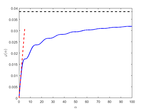
The function is plotted for in Figure 2. As it can be appreciated, roughly looks like a concave function, but not quite: at regular intervals, the slope of the function becomes very small. Such ‘steps’ seem to decrease in amplitude as grows, and, actually, for , the function appears to be well approximated by the ansatz .
To grasp the maximum quantum advantage, we need to study the limiting case . The problem thus consists in determining the spectrum of , restricted to the space . To study this case, it is convenient to switch to the Wigner function representation.
The Wigner function of a quantum state is
For convenience, we recall the properties of Wigner functions in Appendix A. The most important one for us is the fact that Wigner functions behave nicely under metaplectic transformations in phase space. Namely, for any metaplectic transformation , it holds that
| (6) |
Furthermore, for any bounded measurable function and , we have that
| (7) |
where some care has to go into the precise meaning of the integral whenever the integrand is not Lebesgue integrable. Finally, note that, if has a convex support in either position or momentum, then the support of its Wigner function corresponding to that variable is also contained in .
Now, for any state , we have, by eq. (7), that
The last factor on the integrand will vanish everywhere, except in the regions , where it equals , and , where it equals . However, if , then , for . Since implies , it follows that the first region does not contribute to the integration above. Hence,
The problem of integrating Wigner functions over wedges (without any further constraints) was studied by Werner Werner 1988 in the context of time-of-arrival operators. The idea is that all wedges can be taken to each other via a metaplectic transformation, and therefore it suffices to study the wedge . Under this transformation, becomes
where we have used that is the space of states that satisfy the condition . Werner considers the operator corresponding to integrating Wigner functions over the quadrant , and determines its spectrum to be . Therefore, . This bound, however, does not take into consideration the constraint . To account for it, we add to Werner’s operator a linear combination of operators corresponding to integrating Wigner functions over hyperbolic regions in the quadrant . Since our Wigner functions vanish in that quadrant, the infimum of the spectrum of the new operator (which can also be determined with the techniques in Werner 1988) also provides an upper bound for . We numerically find the bound , see Appendix D.
In addition, via variational methods, we show that . This figure is obtained by optimizing linear combinations of the average values of the operators , over density matrices with support on the first number states , i.e., , see Appendix C for details. A plot of the Wigner function of a quantum state approximately in and approximately achieving this value can be found in Figure 3 (left).
In the next section, we will show that , the Bracken-Melloy constant Bracken and Melloy 1994, which is conjectured to have the value Penz et al. 2005; Eveson et al. 2005. Our bounds therefore support this widespread belief.
III Connection with other quantum mechanical effects
| Scenario | Operator | Set of states | |||
|---|---|---|---|---|---|
| Standard problem | |||||
| Ultrafast projectile | |||||
| Ultraslow projectile | |||||
| Quantum backflow |
As we have seen, the ultrafast (ultraslow) projectile problem is equivalent to the standard problem, since a unitary (anti-unitary) transformation takes us from the latter to the former. We next see that the standard projectile problem is similarly connected to the most extreme manifestation of other quantum mechanical effects. The exact correspondences are summarized in Table 1. The question of understanding the relation between some of these effects was raised in Goussev 2019 and partially answered in Goussev 2020. Our results answer the challenge posed in Goussev 2019 from a different point of view, namely, that of (anti-)unitary equivalence, and extend the connection to other mechanical effects.
Let us start with the phenomenon of quantum backflow Allcock 1969; Bracken and Melloy 1994; Albarelli et al. 2016; Eveson et al. 2005. Consider a pure state that only has positive momentum and that is evolving freely. In position representation, we can write it as
for some function such that . The probability flux at the origin is therefore
and thus the integrated flux at the origin from time to time is
Note the similarity with eq. (5). Guided by classical intuition, one would expect this integrated flux to be non-negative, since the particle is only moving to the right. However, for some quantum states , this magnitude can be negative: in that case, we speak of quantum backflow.
Alternatively, we can interpret quantum backflow as a decrease in the probability of detecting a particle with positive momentum in the region . This is so because, by the continuity equation
the integrated flux satisfies:
where and .
Call the space of all states with positive momentum support. From all the above it follows that the maximum amount of backflow is given by
where we used the identity . The number , known in the literature as the Bracken-Melloy constant Bracken and Melloy 1994, is thus the solution a problem of the form , for some space of states and some operator . In fact, this problem can be obtained from the standard problem with via the anti-metaplectic transformation . Therefore, .
Going through the literature on quantum backflow, one finds that is conjectured to have the value Penz et al. 2005; Eveson et al. 2005. A figure of is obtained in Eveson et al. 2005 by fitting many points of (an approximation to) the graph of with the ansatz and, a figure of is obtained in Penz et al. 2005, by fitting such points to a degree polynomial over . To our knowledge, prior to our work there were no rigorous, non-trivial upper bounds on , and the best lower bound fell short of the conjectured value of the constant Halliwell et al. 2013. Our results in the preceding section hence give mathematical support to the conjecture .
| Scenario | Operator | Set of states | |||
|---|---|---|---|---|---|
| Extended standard problem with | |||||
| Generalized Quantum Backflow | |||||
| Constant force QB | |||||
| Quantum reentry |
In Table 2 we present another set of quantum effects that are mathematically equivalent, not to the standard problem, but to the extended standard problem with , which we express, via the transformation , as an optimization of over the set of states .
One of these effects is a variant of quantum backflow in which the particle evolves in the presence of a constant force Melloy and Bracken 1998. That is, with the Hamiltonian given by . In Goussev 2019 Goussev proves that this effect is at the same time equivalent to something he calls quantum reentry. Quantum reentry is an effect that consists in preparing a particle in , letting it evolve and then measuring a negative probability flow in some point . That is, the quantity under consideration is for some , which can again be easily transformed to the semi-infinite standard problem, as also shown in Table 2. In particular, the maximum probability transfer in both these effects is the same.
Finally, we note that the extended standard problem is equivalent to computing the maximum expression of quantum backflow when the initial momentum is in the region for some , as shown in Table 2. Thus, when the initial momentum is in this region, the probability “backflow” acts as if there were a constant force acting on the system, since these two problems are again equivalent. This seems to have gone unnoticed by Bracken, who studied the former effect in Bracken 2021, despite having studied the latter in Melloy and Bracken 1998 together with Melloy.


IV Classical vs. quantum rockets
The low value of constitutes a severe obstruction to any practical application of quantum systems for transportation tasks. How to overcome this limit? A tempting idea is to consider scenarios where a transiting quantum projectile launches a second quantum projectile. Iterating this procedure, we arrive at the notion of a quantum rocket, i.e., a quantum mechanical system that, from time to time, throws away some fuel mass in the direction opposite to the intended motion. Since this rocket scenario encompasses the quantum projectile scenario, its maximum quantum advantage is lower-bounded by the Bracken-Melloy constant. Furthermore, one would imagine that, should we prepare the fuel in the right quantum state, the limited quantum advantage present in quantum projectiles could be somehow bootstrapped, hence increasing the overall advantage of the quantum rocket with respect to a classical rocket whose fuel combustion has an identical momentum distribution.
Unfortunately, this is not the case, at least for a large class of quantum rockets. Consider a minimal model for a quantum rocket, where, at time , the rocket itself is regarded as a -dimensional particle of mass and zero spin. The state of the rocket at time is therefore specified through a trace-class positive semidefinite operator . For most of its flight, the rocket will be propagated by the kinetic Hamiltonian . At times , though, the rocket’s free evolution is interrupted: namely, at time the rocket burns and releases a predetermined amount of fuel instantaneously, thus decreasing its overall mass by the same amount.
To model the instantaneous combustion of fuel of mass , we consider a completely positive trace-preserving (CPTP) map that, acting on the rocket’s state , returns a density matrix representing the joint state of the fuel and that of the rest of the rocket , whose mass is now , see Figure 4.
Call () the absolute position and momentum operators of the fuel (the rest of the rocket), and let () denote the canonical variables of the center of mass (the relative coordinates between systems and ), with:
| (8) |
Let be the (symplectic) unitary that switches between the and representations and define . Since is an internal and instantaneous operation, it cannot modify the rocket’s center of mass degree of freedom. This means that . For , this last relation implies that , for some quantum state .
However, must be independent of . Otherwise, one could find two non-orthogonal vectors with the property that are more easily distinguishable than , which contradicts the contractivity of the trace norm under CPTP maps. Putting all together, we find that any rocket-fuel splitting map must be of the form
| (9) |
where is the state of the relative system rocket-fuel. It must be noted that should have been prepared in the rocket’s combustion chamber. If we assume that the combustion chamber is centered in the rocket’s center of mass and has length , then must have spatial support in .
In describing the overall flight of the rocket, we assume that, at time , the quantum rocket, with mass , will release a mass of fuel in state (in the relative frame of reference). Hence, the mass and state of the rocket will be instantaneously updated to , .
We consider the probability to find the rocket at time in the region . This is to be compared with the maximum probability that an analog classical rocket arrives at the same region in time . Like in the projectile scenario, this classical rocket is assumed to have, at time , the same initial mass, initial momentum distribution and initial spatial support as the quantum one. At time , this classical rocket will burn a mass of fuel, and the phase space distribution of the classical fuel in the fuel’s reference frame relative to the rocket is demanded to have the same momentum distribution and spatial support as .
In these conditions, in Appendix E we show that the difference between the quantum and classical arrival probabilities is also limited by . This no-go result crucially relies on eq. (9), which expresses the assumption that the fuel’s interaction with the rocket is instantaneous. Physically, this corresponds to a configuration where the combustion chamber is open on both sides, i.e., the fuel is allowed to exit the rocket, not only against the rocket’s direction of motion, but also towards it. Assumption eq. (9) allows us to map the computation of the rocket’s maximum quantum advantage to the standard problem (with further state constraints) through a metaplectic transformation.
V A transportation scenario with a quantum advantage that supersedes the Bracken-Melloy constant
In view of the last result, it would be reasonable not to expect significant gaps between the arrival probabilities of quantum and classical particles. As it turns out, though, a simple variation of the way we compare classical and quantum projectiles is enough to find quantum advantages for transportation way beyond the Bracken-Melloy constant. Note that there exist known variations of the quantum backflow problem that achieve quantum advantages greater than the limit set by Bracken and Melloy Goussev 2020; Goussev 2021; Strange 2012; Barbier et al. 2023. Those effects are, however, unrelated to transportation tasks.
In Section II, we compared the behavior of a quantum projectile (or a rocket) with respect to that of a classical one with the same momentum distribution and the same spatial support at time . Could the quantum advantage be amplified if we demanded further constraints on the initial position distribution of the classical projectile, besides its support? In the extreme case, we could demand to coincide with the position distribution of the quantum projectile.
Consider thus the following problem: let denote the density matrix of a particle of mass , and let be its position and momentum distributions at time . As before, we let the projectile evolve freely for time and then check whether the projectile is in ; call the corresponding probability. How much does differ from the maximum arrival probability of an analog classical particle, with initial position and momentum distributions ?
The maximum classical probability of arrival is
| (10) | ||||
where represents the probability distribution of the classical particle in phase space at time .
The maximum quantum-to-classical advantage in this projectile scenario is therefore , where . This is a nested max-min optimization problem, whose solution can be proven independent of 22 2 This can be shown by replacing by in , where is the metaplectic transformation , ..
In Appendix F, is shown to equal , the solution of the system of ordinary differential equations
| (11) |
with initial conditions . Here is meant to be for and otherwise. can be computed numerically via, e.g., Euler’s explicit method.
Since we know how to compute , one could, in principle, use gradient ascent methods to find the maximum of , over all quantum states with, say, support on the space spanned by the first number basis vectors. That is, we could parametrize any such state as and then follow the gradient of with respect to the variables . Unfortunately, is a concave function, so the method is not guaranteed to converge to the absolute maximum. Moreover, we empirically observe that, starting from a random state, projected gradient methods typically converge to very suboptimal values.
To find a suitable starting point for gradient ascent, we considered the following approach: suppose that there existed a linear operator such that
| (12) |
for all states . Then we could maximize the value
| (13) |
over all density matrices with support on the first number states. The result would provide us with a lower bound on . In addition, if the maximizer satisfied , then that state would be a good starting point for gradient ascent.
Now, how to identify an operator satisfying (12)? Let be two functions such that
| (14) |
for all . Then, for any distribution in phase space with marginals ,
| (15) |
It follows that the operator fulfills condition (12). In fact, the dual of problem (10) is the maximum of the right-hand side of eq. (15) over all such functions .
Take . We observe that the functions satisfy (14), and hence, the supremum of the spectrum of the operator provides us with a lower bound for , as .
If we truncate this operator in the number basis, we are looking at the maximum eigenvalue of the matrix , with
For , the maximum eigenvalue of this matrix is : the reader can find a plot of the Wigner function of the corresponding eigenvector in Figure 3 (right). Taking , we obtain the tighter bound . The maximum quantum advantage in this projectile scenario is therefore substantially greater than the conjectured value of , or even its upper bound , derived in section II.1.
Applying gradient methods on those states to improve their value proved to be tricky, though. Call the state corresponding to the eigenvector of . We observe that, even for low values of (say, ), we need to use a very small step size in eq. (11) to estimate precisely. When we do so, we find that : that is, for such quantum states, our upper bound (12) on is (approximately) tight. Around the eigenvectors of , the gradient of explodes, possibly because the function is not everywhere differentiable. Using random perturbations of as a seed, projected gradient methods only produced states with a objective value slightly smaller than .
From all the above, it is thus natural to conjecture that the obtained value of is (close to) a local maximum of , at least among quantum states with support in .
On the other hand, note that after a suitable metaplectic transformation the problem becomes , where
with . The operator is the one studied by Tsirelson in Tsirelson 2006. The best known bounds for its spectrum are given in Zaw et al. 2022. Using Equation (D20) in Zaw et al. 2022, one obtains that . In particular, this shows how unreliable the numerical estimation of these quantities is, even after using a basis with number states, and thus the importance of getting good upper bounds as well as lower bounds.
VI Conclusion
In this letter, we have investigated how the dynamics of quantum and classical projectiles differ, using the probability of arrival at a distant region of space as a figure of merit. We found that non-relativistic quantum particles can arrive at a distant region with higher or lower probability than any classical particle with the same initial spatial support and momentum distribution. Curiously enough, the maximum gap between quantum and classical probabilities is independent of the distance to the arrival region, and just depends on the mass and spatial support of the projectile and its flying time through the single parameter .
The discrepancy between the quantum and classical arrival probabilities is, however, limited by the Bracken-Melloy constant . As we showed, the maximum quantum advantage of rockets with an open combustion chamber is also bounded by this value. Our no-go result does not apply, however, to rockets with a -side closed combustion chamber, which just allows the fuel to exit the rocket opposite to its direction of motion. Whether such rocket models are also limited by , or on the contrary, they can achieve arrival probabilities much higher than classical is an interesting topic for future research.
In a similar direction, we showed that considerable quantum-classical gaps of at least can be observed if we demand classical projectiles to reproduce the initial position distribution of the quantum projectile. It is an open problem whether this figure is indeed close to the maximum quantum advantage, and whether this effect can be exploited for real transportation tasks.
Acknowledgements
We thank Valerio Scarani for interesting discussions, Reinhard Werner for pointing us to reference Werner 1988, and Zaw Lin Htoo for pointing to us that using (D20) of Zaw et al. 2022 one can slightly improve our numerical bound of Section V. D.T. is a recipient of a DOC Fellowship of the Austrian Academy of Sciences at the Institute of Quantum Optics and Quantum Information (IQOQI), Vienna. T.P.L is supported by the Lise Meitner Fellowship of the Austrian Academy of Sciences (project number M 2812-N).
Competing Interests The Authors declare no Competing Financial or Non-Financial Interests.
Author Contributions All authors contributed equally to the research and writing.
Data availability There is no data set in this work.
Disclaimer This version of the article has been accepted for publication, after peer review but is not the Version of Record and does not reflect post-acceptance improvements, or any corrections. The Version of Record is available online at: https://doi.org/10.1038/s41534-023-00739-z.
References
- Razavy (2013) M. Razavy, Quantum theory of tunneling (World Scientific, 2013).
- Allcock (1969) G. Allcock, The time of arrival in quantum mechanics ii. the individual measurement, Annals of Physics 53, 286 (1969).
- Bracken and Melloy (1994) A. J. Bracken and G. F. Melloy, Probability backflow and a new dimensionless quantum number, Journal of Physics A: Mathematical and General 27, 2197 (1994).
- Tsirelson (2006) B. Tsirelson, How often is the coordinate of a harmonic oscillator positive? (2006), arXiv:quant-ph/0611147 [quant-ph] .
- Zaw et al. (2022) L. H. Zaw, C. C. Aw, Z. Lasmar, and V. Scarani, Detecting quantumness in uniform precessions, Physical Review A 106 (2022).
- Muga et al. (2007) G. Muga, R. S. Mayato, and I. Egusquiza, Time in quantum mechanics, Vol. 734 (Springer Science & Business Media, 2007).
- Penz et al. (2005) M. Penz, G. Grübl, S. Kreidl, and P. Wagner, A new approach to quantum backflow, Journal of Physics A: Mathematical and General 39, 423 (2005).
- Eveson et al. (2005) S. P. Eveson, C. Fewster, and R. Verch, Quantum inequalities in quantum mechanics, Ann. Henri Poincaré 6, 1 (2005).
- Palmero et al. (2013) M. Palmero, E. Torrontegui, J. G. Muga, and M. Modugno, Detecting quantum backflow by the density of a bose-einstein condensate, Physical Review A 87, 053618 (2013).
- Eliezer et al. (2020) Y. Eliezer, T. Zacharias, and A. Bahabad, Observation of optical backflow, Optica 7, 72 (2020).
- Barbier and Goussev (2021) M. Barbier and A. Goussev, On the experiment-friendly formulation of quantum backflow, Quantum 5, 536 (2021).
- Miller et al. (2021) M. Miller, W. C. Yuan, R. Dumke, and T. Paterek, Experiment-friendly formulation of quantum backflow, Quantum 5, 379 (2021).
- Daniel et al. (2022) A. Daniel, B. Ghosh, B. Gorzkowski, and R. Lapkiewicz, Demonstrating backflow in classical two beams’ interference, New Journal of Physics 24, 123011 (2022).
- (14) The identity is a consequence of the formulas , .
- Bracken (2021) A. J. Bracken, Probability flow for a free particle: new quantum effects, Physica Scripta 96, 045201 (2021).
- Werner (1988) R. F. Werner, Wigner quantisation of arrival time and oscillator phase, Journal of Physics A: Mathematical and General 21, 4565 (1988).
- Goussev (2019) A. Goussev, Equivalence between quantum backflow and classically forbidden probability flow in a diffraction-in-time problem, Physical Review A 99, 043626 (2019).
- Goussev (2020) A. Goussev, Probability backflow for correlated quantum states, Phys. Rev. Res. 2, 033206 (2020).
- Albarelli et al. (2016) F. Albarelli, T. Guaita, and M. G. Paris, Quantum backflow effect and nonclassicality, International Journal of Quantum Information 14, 1650032 (2016).
- Halliwell et al. (2013) J. J. Halliwell, E. Gillman, O. Lennon, M. Patel, and I. Ramirez, Quantum backflow states from eigenstates of the regularized current operator, Journal of Physics A: Mathematical and Theoretical 46, 475303 (2013).
- Melloy and Bracken (1998) G. Melloy and A. Bracken, The velocity of probability transport in quantum mechanics, Annalen der Physik 510, 726 (1998).
- Goussev (2021) A. Goussev, Quantum backflow in a ring, Physical Review A 103, 022217 (2021).
- Strange (2012) P. Strange, Large quantum probability backflow and the azimuthal angle–angular momentum uncertainty relation for an electron in a constant magnetic field, European journal of physics 33, 1147 (2012).
- Barbier et al. (2023) M. Barbier, A. Goussev, and S. C. L. Srivastava, Unbounded quantum backflow in two dimensions, Phys. Rev. A 107, 032204 (2023).
- (25) This can be shown by replacing by in , where is the metaplectic transformation , .
- Voros (1977) A. Voros, Asymptotic Kappa-Expansions of Stationary Quantum States, Ann. Inst. H. Poincare Phys. Theor. 26, 343 (1977).
- Littlejohn (1986) R. G. Littlejohn, The semiclassical evolution of wave packets, Physics Reports 138, 193 (1986).
- Brask (2021) J. B. Brask, Gaussian states and operations – a quick reference (2021).
- Abramowitz and Stegun (1964) M. Abramowitz and I. A. Stegun, Handbook of Mathematical Functions with Formulas, Graphs, and Mathematical Tables, ninth dover printing, tenth gpo printing ed. (Dover, New York, 1964).
- Wood and Bracken (2005) J. Wood and A. Bracken, Bounds on integrals of the wigner function: The hyperbolic case, Journal of mathematical physics 46, 042103 (2005).
- Vandenberghe and Boyd (1996) L. Vandenberghe and S. Boyd, Semidefinite programming, SIAM Review 38, 49 (1996).
- Löfberg (2004) J. Löfberg, Yalmip : A toolbox for modeling and optimization in matlab, in Proceedings of the CACSD Conference (Taipei, Taiwan, 2004).
- (33) L. Vandenberghe and S. Boyd, The MOSEK optimization toolbox for MATLAB manual. Version 7.0 (Revision 140). (MOSEK ApS, Denmark.).
VII Appendix
In this Appendix we perform some of the lengthy computations that give the claims of the main text. It is organized as follows. In section A, we review the relevant properties of the Wigner function. In section B we give an explicit formula for and show how to numerically approximate it for finite . In section C we compute a numerical lower bound for . In section D we compute a numerical upper bound for . Section E proves that there is no advantage in our model of the quantum rocket with respect to a single projectile. Finally, in section F we describe the numerical methods used in the restricted projectile scenario.
Appendix A Notes on the Wigner function
The Wigner function of a quantum state is
This is a partial Fourier transform on the function , and as such is defined with the usual density arguments from the states such that is a Schwarz function of two variables.
We now study the action of metaplectic transformations on the Wigner function. Suppose then that is affine-linear, and . Then, calling the linear part of , we must conclude that . It is well known that , which gives rise to the name metaplectic that we have used in the main text. Furthermore, the KAN decomposition of is
That is, every matrix decomposes as a product of a rotation, a dilation and a translation. These all correspond to time evolutions of quadratic Hamiltonians (, and or , respectively). Finally, the affine part of the map can be realized by time-evolving with the Hamiltonians and . These six Hamiltonians thus give rise to the unitaries mentioned in the main text.
On the other hand, since all such Hamiltonians are at most quadratic in momentum and position, the time evolution of the Wigner function must satisfy the Liouville equation Voros 1977; Littlejohn 1986, i.e., it must evolve classically in phase space. Therefore,
as the main text claims.
If, on the other hand, , then there is an extra matrix
in the KAN decomposition of the linear part of . This operator corresponds to the antiunitary map , where denotes complex conjugation in the position basis. Indeed, a short computation shows that
Given an operator , we define its Wigner function as
With these choices of normalization, a short computation shows that
In the main text we are primarily concerned with operators of the form for some bounded measurable function . We now prove that
| (16) |
Since is bounded and measurable, we have that (as a tempered distribution) it has an inverse Fourier transform , and we may write . Via functional calculus, we thus have
where we have used the Baker-Campbell-Haussdorf formula . A straightforward computation now shows that
from which we conclude the result.
Since it will be useful soon, we next compute the Wigner function of the operator , in number basis, i.e., . First note that, by linearity of the Wigner function, for any state , we have that
| (17) |
Now, take to be a coherent state, i.e., , with
| (18) |
It follows that
| (19) |
On the other hand, the Wigner function of a coherent state is known to be Brask 2021
| (20) |
with . Cancelling the factor in both sides of (17) and expanding the remaining exponential in (20) as a power series in , we can compare the coefficients multiplying on both sides of the resulting equation, thus obtaining
| (21) | ||||
Note that in Tsirelson 2006 Tsirelson provides the complex conjugated formula for the same quantity. This mistake does not, however, invalidate the main result of Tsirelson 2006, namely, the computation of the spectrum of a given linear operator. This is so because the spectra of a self-adjoint operator and its complex conjugate in a given basis coincide.
Next, we invoke (21) to derive the matrix elements and show that
| (22) |
We will use this expression in Appendices C, F to lower bound the maximum quantum advantage in the standard and restricted projectile scenarios.
To begin, from eq. (16) we have that
| (23) |
We can evaluate the right-hand side of the above equation by changing to polar coordinates. The result is
| (24) |
with
| (25) |
where, in the last step, we changed the sum variable so that a comparison with eq. (1.5) in Tsirelson 2006 can be made.
As it turns out, the final expression for can be written in terms of the generalized hypergeometric function . Thanks to such an identity, we were able to compute accurately for large values of .
Appendix B Properties of
First, we will calculate the kernel of in position representation. Our starting point is the identity
| (26) |
where the integral must be understood as a Cauchy principal value. Thus we have that
| (27) |
To arrive at the final expression, we invoked the Baker-Campbell-Haussdorf formula in the first line; the resolution of the identity , in the second one; the relation (assuming that the bra is an element of the position basis; and the ket, of momentum basis), in the third one; and the relation , in the fourth one.
Using the same techniques, one finds that
| (28) |
Hence we have that
| (29) |
This expression can be further reduced to a real kernel by conjugating it with the unitary , which results in the operator
| (30) |
where .
B.0.1 Bounding
We start from the easily verifiable identity:
| (31) |
Applying the identity to eq. (30), we find that
| (32) |
with
| (33) |
Define . Note that , where the unitary leaves invariant. Now, by eq. (32), we have that
| (34) |
On the other hand, when averaged over elements of , has support on a two-dimensional subspace, namely, the span of the vectors
| (35) |
The maximum eigenvalue of is therefore the result of solving the generalized eigenvalue problem with matrices given by
| (36) |
The result is the upper bound on
| (37) |
As shown in Figure 2 (main text), this analytic (and linear) bound is very good for small values of .
To arrive at better approximations for , we will exploit the fact that the integrand in (30) is an analytic function; and the spatial support of the states in , finite. Consider an operator of the form
| (38) |
with analytic in . Then, for any , one can find such that the -order Taylor expansion of satisfies , for . Define thus the operator
| (39) |
and let . Then,
| (40) |
where denotes the normalized state with wave-function . The maximum eigenvalue of is therefore an -approximation to the top of the spectrum of . Note, as we did in deriving the upper bound on , that has support on the finite set of vectors
| (41) |
hence in principle we can diagonalize it exactly. In practice, though, the Gram matrix of the vectors in is ill-conditioned, so, with computer precision, one can just diagonalize reliably for low values of . To overcome this difficulty, we exploit the properties of the Legendre polynomials Abramowitz and Stegun 1964.
The Legendre polynomials are o rthogonal in the interval with respect to the weight . It follows that are orthogonal in the interval . Invoking the formula for the scalar product of Legendre polynomials Abramowitz and Stegun 1964, and taking into account the compression , we have that
| (42) |
In addition, Legendre polynomials satisfy the recurrence relation Abramowitz and Stegun 1964
| (43) |
From the identity , we hence arrive at a simple expression for the expansion of the monomials in the polynomial basis :
| (44) |
where is the matrix with rows and columns numbered from to and non-zero coefficients
| (45) |
Call the Gram matrix of the basis functions , i.e., . From the above it follows that
| (46) |
Diagonalizing thus entails solving the generalized eigenvalue problem
| s.t. | (47) |
Defining , we find that our -approximation to the maximum eigenvalue of is the maximum eigenvalue of the matrix .
Let us apply these considerations to the operator (30). In this case, . By Taylor’s remainder theorem, we have that, for any ,
| (48) |
for some . It follows that, for , the following relation holds:
| (49) |
Using Stirling’s approximation , we conclude that, in order to compute up to error , the following condition must be fulfilled:
| (50) |
A sufficient condition to satisfy this relation is that and .
Appendix C Lower bounds on
To improve the lower bounds on obtained through the exact computation of for high values of , we will follow a variational approach. Recall that is the result of maximizing over all quantum states . Hence, any quantum state satisfying this constraint gives a lower bound on . For any , we can enforce this constraint by projection:
| (51) |
with . Using , it is easy to prove that, for ,
| (52) |
which provides a way to lower bound , given an arbitrary quantum state not necessarily in .
Appendix D Upper bounds on
As explained in the main text, the problem of upper bounding is equivalent to that of lower bounding the bottom of the spectrum of the operator defined through , constrained to the space of wave-functions satisfying .
Restricted to this space, , for any operator that integrates a Wigner function on some region . Therefore,
Unfortunately, computing integrals of Wigner functions on arbitrary regions of phase space is arbitrarily complicated, so we must restrict ourselves to tractable regions.
Define . Such hyperbolic regions are invariant under the action of the dilation group , and it turns out that the operator representing integration over can be block-diagonalized in a basis of dilation eigenvectors, exactly like Werner does for in Werner 1988. The hyperbolic regions were independently considered in full generality in Wood and Bracken 2005, where the spectrum is also numerically computed. The result can only be expressed as follows in terms of integrals which do not have an analytical expression, as far as we are aware:
where
As proven in Werner 1988, the operator is block-diagonalized by the same unitary transformation. Setting , we thus have that the bottom of the spectrum of equals , where denotes the minimum eigenvalue of the matrix and is a one-parameter of matrices.
In this regard, the best combination we could find before the integrals defining the entries of became too numerically unstable to be reliable is
whose spectrum as a function of is shown in Figure 5.

Appendix E Quantum rockets
Under the assumption that the map (9) describes fuel combustion, consider a rocket that, most of the time, freely propagates through space, except at times , when the rocket burns fuel instantaneously. We assume that, initially, the state of the rocket’s center of mass is , with canonical operators . At time , the rocket burns a fuel mass , hence reducing its mass to , and experiencing a transformation , where of the fuel in the rocket’s reference frame, with canonical operators . Between the times and , the rocket propagates freely and thus its canonical operators experience the transformation
| (54) |
Call the canonical operators of the rocket at time , just before the new fuel combustion. From eqs. (8), (54) it is easy to see that they satisfy the relation
| (55) |
Through repeated iteration of (55), we can express the rocket’s final position operator as a linear combination of and . That is, for some real vectors , we have , where and . The probability of detecting the quantum rocket at time in and its classical counterpart is thus given by
| (56) |
where . Since eq. (55) also holds for classical systems, so does eq. (56), when we understand as a product of probability densities. We now consider a classical rocket with the same combustion schedule as the quantum one, and such that the probability densities for the classical moment variables respectively coincide with those of the states . We further assume that the distributions of the initial position of the rocket and the fuel explosions respectively have supports and , just like in the quantum case. Then, the maximum probability of detecting the classical rocket in at time is
| (57) |
where
| (58) |
The maximum advantage of such a quantum rocket is thus the result of maximizing
| (59) |
over all separable states such that , , for . Call the corresponding maximizer (if the maximizer does not exist, then the following argument still carries through if the average value of (59) with is ).
Now, consider the commutator , and assume that . Then,
are canonically conjugated operators. Let be the result of tracing out all degrees of freedom of , but that corresponding to . Then we have that
| (60) |
with , with
| (61) |
Hence we end up computing under an extra restriction on the quantum states to be optimized. Through the metaplectic transformation , we can map this problem to an optimization over the operator
| (62) |
over a constrained set of quantum states contained in , with , . This means that .
If , we apply the time-reversal anti-unitary operator , , , on the operator of eq. (59). This transformation does not affect the spatial support or separability of , but effectively changes the sign of ; and thus, of the commutator, in which case the argument above carries through.
Finally, if , then are commuting operators, in which case eq. (59) cannot have a value greater than .
The final conclusion is that a quantum rocket cannot be more advantageous than a quantum projectile.
Appendix F The restricted projectile scenario
F.1 Computation of
In this section, we solve the following problem.
Problem 1.
Let be the position and momentum distributions of a classical particle of mass . What is the maximum probability that, after time , we find the particle in the region ?
In classical mechanics, such a particle is described by its phase space distribution constrained to have position and momentum marginals and . Though our notation is similar to Wigner functions, we emphasize that here is a valid probability distribution. The problem is maximizing over random variables jointly distributed according to with given marginals.
A discretized version of the problem is maximizing the fraction of pairs , sampled from , satisfying . That is to find a permutation maximizing the fraction above. Let , the initial momentum distribution becomes .
Lemma 1.
Given , let the indices be
| (63) |
Then, there exists an optimal permutation such that .
Proof.
Let be a permutation maximizing the number of pairs satisfying . If , then the lemma holds with the permutation . If , then the lemma holds with the permutation , defined by
| (64) |
Indeed, note that the transition just affects the pairs
| (65) |
By definition of , if the second pair adds up to or more, then . In that case, the transition will make both final pairs add up to or more. On the contrary, if the second pair adds up to a number lower than , this means that, at most, just the first pair was satisfying the sum condition. After the transition, though, the pair satisfies it by definition. So once again the transition cannot decrease the number of pairs satisfying the sum condition.
It follows that is optimal if is optimal. Since , the conditions of the lemma are satisfied. ∎
The lemma suggests a simple algorithm to arrive at an optimal permutation , given the vectors . Namely,
- 1.
Define , .
- 2.
Find such that
(66) If no such indices exist, return any permutation with and halt.
- 3.
Redefine , and go to 2.
To solve the problem posed at the beginning of the section, we just need to apply the algorithm above in a scenario where . In that limit, the quantities approximate the number of entries of with values in and .
Suppose that we have already paired or discarded all entries of with value smaller than or equal to . Call the number of pairs already established and , the number of elements of which are still unpaired and are greater than or equal to . Following the algorithm, we need to check how many of the points with value in we can pair with the remaining entries of . The only possible candidates in are either among the entries already counted in or among the entries with values in . If , then all the entries with values in can be paired, i.e., . In that case, after removing those, the remaining entries of vector are in the interval . Also, the number of unpaired elements of greater than are , with . If , then there are two possibilities: (1) , in which case entries can be paired, and so , ; (2) , in which case just can be paired, and so , . Defining , , we hence have that the functions follow the system of differential equations
| (67) |
F.2 The gradient of
Suppose that the distributions depend on one parameter , i.e., . We wonder how much differs from , with . Let us assume that the roots of can be expressed as , with , for all . Then,
| (68) |
where if , and
| (69) |
An increment of will thus have two effects on . On one hand, the functions will respectively change by the amounts , . On the other hand, the set of points where vanishes will change. Assuming that the kernel of is of the form , then we have that
| (70) |
From eqs. (67), and, assuming that are smooth, we have that
| (71) |
Indeed, if this quantity were negative, then would have remained zero; and, if it were positive, then there would exist such that , and would have lifted itself from zero at instead of . By (69), this implies that the last term of eq. (70) vanishes.
As for the second-to-last term, from eq. (67) it follows that, for , ,
| (72) |
where we have used the identities and (71). Equaling this last equation to zero, we find that
| (73) |
Define
| (74) |
From eqs. (70), (73), we find that , where the function and the auxiliary function evolve according to the system of ordinary differential equations
| (75) |
for , and otherwise are updated as indicated below (notice the update order):
| (76) |
Here, the boundary conditions are . Note that the first line of (75) is the same as the second line of (67). Hence it is advisable to run the algorithm to find and its differential at the same time. Also, notice that the algorithm sometimes requires us to differentiate a non-differentiable function, such as . In that case, we define as , if ; or , otherwise. In doing so, we are implicitly assuming that the equation has a countable number of roots in . The definition of is analogous.
F.3 Maximizing
Since the maximum quantum advantage is independent of the parameters , from now on we take , in that is
| (77) |
We will only perform projected gradient ascend in the subspace , noting that we can get better achievable lower bounds with increasing number of iterations and increasing . For a learning rate , each iteration updates the state according to
| (78) |
with the projection ensuring a valid density matrix. It remains to compute various quantities above.
Firstly, for any matrix , the projection to the set of density matrix can be cast as a semidefinite program Vandenberghe and Boyd 1996:
| s.t. | ||||
| (81) |
To solve this program, we used the MATLAB package YALMIP Löfberg 2004 in combination with the semidefinite programming solver MOSEK Vandenberghe and Boyd.
Next, . Write
| (82) |
and let be our real variables to be optimized. Then the first term
| (83) |
where is the matrix with entries given by (24) for .
Finally, the last term consists of individual gradients , in the notation of the previous section, receiving contribution from the gradient with respect to real parameters . Call the set of complex matrices. From (75) and (76), we have for the solution of
| (84) |
for , and otherwise are updated as
| (85) |
This system of differential equations contains auxiliary functions and to be solved, as well as data functions depending on parameters and their gradients. Recalling their definitions, we get that their gradients depends on
| (86) |
where are the -dimensional vectors with entries , for and
| (87) |
where denotes the Hermite polynomial of degree , defined by
| (88) |
In summary, we have completely specify the data defining the system of differential equations, as well as the computation leading to the update (78).
To solve the above system of ordinary differential equations, as well as (67), we used the Euler explicit method with step . For practical reasons, we had to limit the range of possible values of , which we set to be .