Nonlinear spectroscopy of bound states in perturbed Ising spin chains

Introduction. Spectroscopic tools have played a crucial role in our understanding of complex quantum systems Devereaux and Hackl 2007. However, we can only partially measure their correlations with existing tools. Terahertz 2D coherent spectroscopy, one of developing spectroscopic tools  Shen 1984; Hamm and Zanni 2011; Mukamel 1999, stands out as a technique for a deeper understanding of strongly-correlated condensed matter systems. It probes the nonlinear optical response which has been used to identify the ground state symmetry of magnetic Fiebig et al. 2005 and superconducting Chu et al. 2020; Schwarz et al. 2020 materials, geometric phase in topological materials Wu et al. 2017; Shao et al. 2021; He et al. 2021, novel ground states in correlated systems Zhao et al. 2017; Zhao et al. 2016, and quasiparticle decay processes in a disordered system Mahmood et al. 2021. Besides, recent experimental advances with terahertz sources put the technique in a proper energy range to study rotational dynamics in molecules Lu et al. 2016, spin waves in conventional magnets Lu et al. 2016, and exotic excitations in quantum magnets Wan and Armitage 2019; Li et al. 2021; Choi et al. 2020; Nandkishore et al. 2021; Fava et al. 2021.

In contrast to more common 1D spectroscopy, the 2D extension unravels not only the optical excitations but also their interplay Mukamel 1999; Hamm and Zanni 2011. The advantage of this experimental technique has been widely adopted by chemists to reveal the structure of complex molecules with great success. However, such achievements rely on powerful numerical methods that help to interpret complicated experimental data starting from concrete microscopic models Woutersen et al. 2002; Cho 2008; Terranova and Corcelli 2014. In this regard, it is desirable to develop an efficient numerical platform for future 2D spectroscopy experiments on quantum magnets similar to the successful use of matrix product state (MPS) techniques for conventional 1D spectroscopy Paeckel et al. 2019; Vanderstraeten et al. 2015; Bera et al. 2017; Vanderstraeten et al. 2018; Van Damme et al. 2021; Fava et al. 2020; Morris et al. 2021. However, the calculation of nonlinear response is less explored and the need for multiple time evolutions makes it much more challenging.

In this work, we propose an efficient numerical tool using infinite MPS (iMPS) and study the nonlinear response of 1D spin model. To benchmark the method, we first focus on the 1D transverse field Ising model (TFIM) whose nonlinear response can be analytically calculated using Jordan-Wigner (JW) transformations Wan and Armitage 2019. Motivated by the quasi-1D structure of $\mathrm{CoNb}_{2}\mathrm{O}_{6}$ – one of the best material example of an Ising chain magnet – (albeit with more complicated magnetic interactions Fava et al. 2020; Morris et al. 2021) we then include longitudinal field terms which capture the effects of inter-chain interactions and lead to the emergence of confined bound state excitations Lee et al. 2010; Kinross et al. 2014; Xu et al. 2022. As a consequence, new signals appear in 2D spectroscopy which include strong non-rephasing and rephasing like peaks. Our results from the iMPS method are furthermore corroborated by perturbative calculations starting from the projected two-kink (TK) low energy subspace. We find quantitative agreement in the strongly confined regime, which allows us to understand the origin of sharp peaks in the 2D spectrum as transitions between bound states.

Model. We first introduce the 1D TFIM

with $J,h_{x}>0$. For $h_{x}<h^{c}_{x}=J$, it stabilizes a doubly degenerate ferromagnetic ground state polarized along the easy axis $\hat{z}$. When $h_{x}>h^{c}_{x}$, the system has a unique paramagnetic ground state. In the ferromagnetic regime, the experimental excitation, i.e., a local spin flip, splits into two freely moving kinks (domain-walls) between two degenerate states. In the context of non-linear spectroscopy these fractionalized excitations have been shown to be manifest as sharp signatures in the third order magnetic susceptibilities Wan and Armitage 2019.

We now include a longitudinal field and focus on the Hamiltonian given by $H=H_{0}-h^{z}\sum_{n}\sigma^{z}_{n}$ with $J,h_{x},h_{z}>0$. In the ferromagnetic regime, the longitudinal field lifts the degeneracy and selects one of the polarized ground states. Besides, it induces a linear confining potential between the kinks leading to bound states. As a result, the broad continuum of free kink excitations as probed in linear response fragments into sharp peaks Kjäll et al. 2011. At a low transverse field, the splitting can be understood via a Schrödinger equation for the relative kink separation with a linear potential McCoy and Wu 1978 which can also be generalized to include lattice effects Coldea et al. 2010; Morris et al. 2014; Rutkevich 2010; Rutkevich 2008; Shinkevich and Syljuåsen 2012; Kormos et al. 2017; Liu et al. 2019. The main questions of our work are: How to efficiently simulate the nonlinear response of the TFIM with a longitudinal field using MPS methods? What are the robust signatures of confined bound states in nonlinear 2D spectroscopy?

2D spectroscopy. Here, we introduce a two-pulse protocol which following previous work Ref. Wan and Armitage 2019. In this setup, two Dirac-delta pulses $B_{0}$ and $B_{\tau}$ which are polarized along $\hat{\alpha}$ and $\hat{\beta}$ directions, respectively, reach the sample at time $T=0$ and $T=\tau>0$ successively. These magnetic pulses couple to the local moments of the sample and the induced magnetization along $\hat{\gamma}$ direction is recorded as $M^{\gamma}_{\mathrm{0\tau}}(T)$ at time $T=\tau+t$ where $t>0$ is the time interval between the second pulse $B_{\tau}$ and the measurement. To subtract the signal from the linear response, two different experiments are repeated but with pulse $B_{0}$ or $B_{\tau}$ alone to measure $M^{\gamma}_{0}(T)$ and $M^{\gamma}_{\tau}(T)$. The nonlinear signal field emerging from the sample at $T=\tau+t$ in the $\hat{\gamma}$ direction is defined as

The nonlinear signal depends only on the nonlinear responses and directly measures the second and higher order magnetic susceptibilities Nandkishore et al. 2021:

The 2D spectrum is the Fourier transform of $M^{\gamma}_{\mathrm{NL}}(t,\tau)$ over both time domains $t$ and $\tau$. In Eq. (3), the leading contribution to the nonlinear response in the two-pulse setup, i.e., the second order nonlinear susceptibility $\chi_{\gamma\beta\alpha}^{(2)}(t,\tau+t)$, is given as

with the three point spin correlation function in the ground state $|\psi\rangle$,

where $\sigma^{\gamma}_{j}(T)\equiv e^{iHT}\sigma^{\gamma}_{j}e^{-iHT}$. When the Hamiltonian and $|\psi\rangle$ preserves the lattice translation symmetry, the site index $m$ in Eq. (4) and Eq. (5) can be fixed, e.g. as $c\equiv L/2$ the central site of the system, which we use in the following. Then, $\chi^{(2)}_{\gamma\beta\alpha}(t,\tau+t)$ is obtained by evaluating

Method. A promising tool for calculating $S^{\gamma\beta\alpha}_{j,l,c}(\tau+t,\tau,0)$ in Eq.(6) for a whole range of site indices $j$ and $l$ is to use the iMPS method. We only need to perform two different real time evolution runs to calculate $\sum_{j,l}S^{\gamma\beta\alpha}_{j,l,c}(\tau+t,\tau,0)\!=\!\sum_{j,l}e^{iE(\tau+t)}\langle\psi|\sigma^{\gamma}_{j}e^{-iHt}\sigma^{\beta}_{l}e^{-iH\tau}\sigma^{\alpha}_{c}|\psi\rangle$ where $E$ is the ground state energy. In addition, finite size effects are avoided. Such effect originates from the bouncing of correlations following a local quench at site $j=1$ or $L$, boundary sites of the system. Below, we explain a procedure to obtain $\langle\psi|\sigma^{\gamma}_{j}e^{-iHt}\sigma^{\beta}_{l}e^{-iH\tau}\sigma^{\alpha}_{c}|\psi\rangle$ (See Section I of Supplementary Information (SI) for $S^{\beta\gamma\alpha}_{j,l,c}(\tau,\tau+t,0)$).

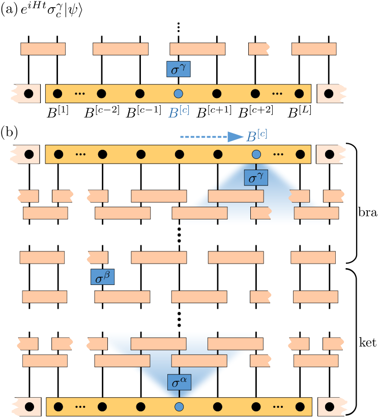
1. 1.

   Find a ground state and perform a time evolution following a local quench, $\sigma_{c}^{\gamma}$ or $\sigma_{c}^{\alpha}$, using infinite time evolving block decimation (iTEBD) methodVidal 2003; Vidal 2004; Vidal 2007 to obtain an iMPS for $e^{iHt}\sigma^{\gamma}_{c}|\psi\rangle$, which is shown in Fig. 1(a), or $e^{-iH\tau}\sigma^{\alpha}_{c}|\psi\rangle$.

2. 2.

   Shift every $B$ tensor of an iMPS, which represents $e^{iHt}\sigma^{\gamma}_{c}|\psi\rangle$, $(c-j)$ sites to the right within a window of size $L$ to obtain a new iMPS “bra” associated to $e^{iHt}\sigma^{\gamma}_{j}|\psi\rangle$.

3. 3.

   Apply a local operator $\sigma^{\beta}_{l}$ to an iMPS associated to $e^{-iH\tau}\sigma^{\alpha}_{c}|\psi\rangle$ and get a new iMPS “ket” which represents $\sigma^{\beta}_{l}e^{-iH\tau}\sigma^{\alpha}_{c}|\psi\rangle$.

4. 4.

   Evaluate an overlap of two iMPS “bra” and “ket” within the window by calculating the dominant left and right eigenvector of the corresponding transfer matrix, which is shown in Fig. 1(b), and obtain $\langle\psi|\sigma^{\gamma}_{j}e^{-iHt}\sigma^{\beta}_{l}e^{-iH\tau}\sigma^{\alpha}_{c}|\psi\rangle$ Kjäll et al. 2011.

Before investigating the 2D spectrum of the non-integrable TFIM with longitudinal field, we first focus on the free TFIM and compare the result of $\chi^{(2)}_{xxx}(t,\tau+t)$ using two different schemes, i.e., the numerical iMPS method and analytic calculations via the JW transformation with periodic boundary condition (PBC). Here and below, we set $h_{x}/J=0.2$ and all iMPS simulations are done with a spatial window of size $L=80$ sites and over the time range $Jt,J\tau=30$. Within such temporal range, the light cone spreading of correlations, which follows a local quench at the center of a spatial window, does not reach the boundary of the window. In Fig. 2(a), we plot the result of $\chi^{(2)}_{xxx}(t,\tau+t)$ from the iMPS method. In order to check the errors of our method, we tracked the truncation error, the truncated weight of many-body wave function at each time step in iTEBD, which quantifies an upper limit for the truncation effect on local observables ($\lesssim 10^{-8}$ for every result given in our study). Besides, we also followed the dependence of $\chi^{(2)}_{xxx}(t,\tau+t)$ on the time step $\delta t$ and the bond dimension $\chi$, fixing to $\delta t=0.03/J$ and $\chi_{\text{max}}=30$. In Fig. 2(b), we compare $\chi^{(2)}_{xxx}(t,\tau+t)$ at $Jt=15$ from the iMPS method with the one from the JW formalism which confirms exact agreement. In Fig. 2(c), we plot Re$\chi_{xxx}^{(2)}(\omega_{t},\omega_{\tau})$, the real part of the Fourier transformed $\chi^{(2)}_{xxx}(t,\tau+t)$. It contains a sharp vertical line of intensity centered at $\omega_{t}=0$. Regarding $\omega_{t}$ and $\omega_{\tau}$ as the detecting and pumping frequencies, the response is known as a rectification signal. It also contains a diffusive, weak non-rephasing signal in the first frequency quadrant, mirroring the energy range of the free TK continuum, which is shown in the inset of Fig. 2(c) Wan and Armitage 2019.

Results. Next, we focus on the 2D spectrum of the 1D TFIM with longitudinal field using the iMPS method. Fig. 3(a) shows the Re$\chi_{xxx}^{(2)}(\omega_{t},\omega_{\tau})$, which is calculated in weakly confined regime with $h_{z}/J=0.03$ (See Section II of SI for the Im$\chi_{xxx}^{(2)}(\omega_{t},\omega_{\tau})$, which is related to the Re$\chi_{xxx}^{(2)}(\omega_{t},\omega_{\tau})$ by the dispersion relationKogan 1963; Caspers 1964; Bassani and Scandolo 1991). This value is similar to the one used in Ref. Coldea et al. 2010 to describe $\mathrm{CoNb}_{2}\mathrm{O}_{6}$. New spectroscopic signals are encoded in $\chi_{xxx}^{(2)}(\omega_{t},\omega_{\tau})$ in the presence of a longitudinal field. First, it contains a dominant non-rephasing signal which appears as diagonal peaks in the first quadrant. At the same time, a weakly diffusive terahertz rectification signal is also detected as a streak along the $\omega_{\tau}$ axis. In Fig. 4(a), we plot Re$\chi_{xxx}^{(2)}(\omega_{t},\omega_{\tau})$ in strongly confined regime with $h_{z}/J=0.4$. Unlike the previous regime, it contains a non-rephasing like signal which appears as strong cross (off-diagonal) peaks in the first quadrant. Besides, a subdominant rephasing like signal appears as cross peaks in the fourth quadrant.

To interpret the 2D spectra, we use a projected TK model and can study the excitations of Eq.(1) perturbatively Rutkevich 2010; Kormos et al. 2017. The idea is to project the full Hilbert space down to the Hilbert space of TK states, where regions of opposite magnetization are separated by the two different domain-walls. In this model, each TK state is represented as $|j,l\rangle\equiv|...\uparrow\uparrow\downarrow_{j}\downarrow...\downarrow\downarrow_{(j+l-1)}\uparrow\uparrow...\rangle$, where $j$ is the starting site of down spins. The TK model has been adopted to phenomenologically understand the confinement of excitations observed in the dynamical (1D) neutron response of $\mathrm{CoNb}_{2}\mathrm{O}_{6}$ Coldea et al. 2010; Rutkevich 2010. The projected model is expected to capture the low-energy excitations of the original model well as long as $h_{x}/J\ll h_{z}/J$. This can be understood by looking into the energy gap between TK states and four-kink states Verdel et al. 2020. The TK Hamiltonian, $\mathcal{H}_{TK}\equiv\mathcal{P}H\mathcal{P}$ with the projector $\mathcal{P}$, acts as follows:

For our translational invariant model, the total momentum $p$ of the bound state is a good quantum number. In the momentum basis $|p,l\rangle=\sum_{j}\exp(ipj)|j,l\rangle$, the Hamiltonian is diagonal in $p$ and acts on $|p,l\rangle$ as

By solving the eigen-equation in Eq. (8) for a given momenta $p$ and a band index $n$, one get TK bound state $|\Phi_{n}(p)\rangle$ with the excitation energy $E_{n}(p)$, which is shown in the inset of Fig. 3(b) and 4(b). (See Section III of SI for details). Then, following Ref. Rutkevich 2010, which calculates the linear response, we find (after some algebraic manipulation)

with

where $C_{n,m}(p)$ is the optical matrix element which depends on band indices $n,m$ and momentum $p$ (See Section III of SI for details).

The interpretation of 2D spectra now becomes transparent: $Q_{1}$ gives rise to diagonal non-rephasing peaks at $\omega_{t},\omega_{\tau}=E_{n}(p)$ and $Q_{2}$ produces dominant terahertz rectification signals at $\omega_{t}=0$ and $\omega_{\tau}=\pm E_{m}(p)$ [Fig. 3(b) and Fig. 4(b)]. In the strongly confined regime, $Q_{3}$ gives rise to dominant cross peaks in the first frequency quadrant originating from the non-rephasing like process [Fig. 4(b)]. To be more precise, such peaks sharply appear at $\omega_{t}\!=\!E_{1}(0)$ and $\omega_{\tau}\!=\!E_{2}(0)$ or $\omega_{t}\!=\!E_{2}(0)$ and $\omega_{\tau}\!=\!E_{1}(0)$, indicating the presence of multiple TK excited states. Such sharp peaks do not appear in the free 1D TFIM, which can be mapped to an independent two-level systems with each having a single excited state Wan and Armitage 2019. $Q_{4}$ contains terms which induce sharp (non-)rephasing like signals in the first (fourth) frequency quadrant which are visible in the strongly confined regime [Fig. 4(b)]. Such signals also originate from the presence of multiple excited states and appear at $\omega_{t}=E_{2}(0)-E_{1}(0)$, an energy gap between first and second excited states, and $\omega_{\tau}=E_{2}(0)$ or $-E_{1}(0)$, see inset.

Conclusions. In the present work, we have developed an iMPS method for calculating the nonlinear response of 1D spin systems. As a demonstration, we calculated the second order susceptibility, which dominates the nonlinear response, for the ferromagnetic 1D TFIM where a single spin flip is fractionalized into two freely moving domain-walls. We benchmarked our numerical results with exact analytical calculations. We then included a longitudinal field, which induces a linear confining potential between kink excitations. In the presence of a longitudial field, the second order susceptibility contains new signals which give rise to strong non-rephasing and rephasing like peaks. To understand the emergence of such signals, we employ a simplified two-kink description, which describes the low-energy excitations in the strongly confined regime, and calculate the second order susceptibility perturbatively. The approximate method captures the nonlinear response of the system in the strongly confined regime and allows for a simple interpretation.

As a future direction, it would be interesting to apply our iMPS method near the quantum critical point between the ferromagnetic and paramagnetic states where a hidden E₈ symmetry emerges Coldea et al. 2010; Kjäll et al. 2011. A crucial question regards then the existence of robust signals in 2D spectrum which detect the emergent symmetry. Regarding the microscopic description and 3D nature of $\textrm{CoNb}_{2}\textrm{O}_{6}$ Coldea et al. 2010; Morris et al. 2014 ($\textrm{BaCo}_{2}\textrm{V}_{2}\textrm{O}_{8}$ Zou et al. 2021; Faure et al. 2018) it would be interesting to study a more quantitative model Fava et al. 2020; Morris et al. 2021 and go beyond simple chains, e.g. by extending these to coupled Ising ladders Morris et al. 2014. Terahertz 2D coherent spectroscopy holds the promise of uncovering the nature of exotic excitations in strongly correlated quantum materials. A challenging but very worthwhile direction will be an extension of our method to quantum magnets beyond one-dimension where the nature of fractionalized excitations and confinement thereof remains poorly understood.

Note added. When finalizing the manuscript, related works appeared that investigate nonlinear response from quasiparticle interactions Fava et al. 2022; Hart and Nandkishore 2022.

References

- Devereaux and Hackl (2007) T. P. Devereaux and R. Hackl, Reviews of modern physics 79, 175 (2007).
- Shen (1984) Y.-R. Shen, Principles of nonlinear optics (Wiley-Interscience, New York, NY, USA, 1984).
- Hamm and Zanni (2011) P. Hamm and M. Zanni, Concepts and methods of 2D infrared spectroscopy (Cambridge University Press, 2011).
- Mukamel (1999) S. Mukamel, Principles of nonlinear optical spectroscopy, 6 (Oxford University Press on Demand, 1999).
- Fiebig et al. (2005) M. Fiebig, V. V. Pavlov, and R. V. Pisarev, JOSA B 22, 96 (2005).
- Chu et al. (2020) H. Chu, M.-J. Kim, K. Katsumi, S. Kovalev, R. D. Dawson, L. Schwarz, N. Yoshikawa, G. Kim, D. Putzky, Z. Z. Li, et al., Nature communications 11, 1 (2020).
- Schwarz et al. (2020) L. Schwarz, B. Fauseweh, N. Tsuji, N. Cheng, N. Bittner, H. Krull, M. Berciu, G. Uhrig, A. Schnyder, S. Kaiser, et al., Nature communications 11, 1 (2020).
- Wu et al. (2017) L. Wu, S. Patankar, T. Morimoto, N. L. Nair, E. Thewalt, A. Little, J. G. Analytis, J. E. Moore, and J. Orenstein, Nature Physics 13, 350 (2017).
- Shao et al. (2021) Y. Shao, R. Jing, S. H. Chae, C. Wang, Z. Sun, E. Emmanouilidou, S. Xu, D. Halbertal, B. Li, A. Rajendran, et al., Proceedings of the National Academy of Sciences 118 (2021).
- He et al. (2021) P. He, H. Isobe, D. Zhu, C.-H. Hsu, L. Fu, and H. Yang, Nature communications 12, 1 (2021).
- Zhao et al. (2017) L. Zhao, C. Belvin, R. Liang, D. Bonn, W. Hardy, N. Armitage, and D. Hsieh, Nature Physics 13, 250 (2017).
- Zhao et al. (2016) L. Zhao, D. Torchinsky, H. Chu, V. Ivanov, R. Lifshitz, R. Flint, T. Qi, G. Cao, and D. Hsieh, Nature Physics 12, 32 (2016).
- Mahmood et al. (2021) F. Mahmood, D. Chaudhuri, S. Gopalakrishnan, R. Nandkishore, and N. Armitage, Nature Physics 17, 627 (2021).
- Lu et al. (2016) J. Lu, Y. Zhang, H. Y. Hwang, B. K. Ofori-Okai, S. Fleischer, and K. A. Nelson, Proceedings of the National Academy of Sciences 113, 11800 (2016).
- Wan and Armitage (2019) Y. Wan and N. Armitage, Physical Review Letters 122, 257401 (2019).
- Li et al. (2021) Z.-L. Li, M. Oshikawa, and Y. Wan, Physical Review X 11, 031035 (2021).
- Choi et al. (2020) W. Choi, K. H. Lee, and Y. B. Kim, Physical Review Letters 124, 117205 (2020).
- Nandkishore et al. (2021) R. M. Nandkishore, W. Choi, and Y. B. Kim, Physical Review Research 3, 013254 (2021).
- Fava et al. (2021) M. Fava, S. Biswas, S. Gopalakrishnan, R. Vasseur, and S. Parameswaran, Proceedings of the National Academy of Sciences 118 (2021).
- Woutersen et al. (2002) S. Woutersen, R. Pfister, P. Hamm, Y. Mu, D. S. Kosov, and G. Stock, The Journal of chemical physics 117, 6833 (2002).
- Cho (2008) M. Cho, Chemical reviews 108, 1331 (2008).
- Terranova and Corcelli (2014) Z. Terranova and S. Corcelli, The Journal of Physical Chemistry B 118, 8264 (2014).
- Paeckel et al. (2019) S. Paeckel, T. Köhler, A. Swoboda, S. R. Manmana, U. Schollwöck, and C. Hubig, Annals of Physics 411, 167998 (2019).
- Vanderstraeten et al. (2015) L. Vanderstraeten, F. Verstraete, and J. Haegeman, Physical Review B 92, 125136 (2015).
- Bera et al. (2017) A. Bera, B. Lake, F. Essler, L. Vanderstraeten, C. Hubig, U. Schollwöck, A. Islam, A. Schneidewind, and D. Quintero-Castro, Physical Review B 96, 054423 (2017).
- Vanderstraeten et al. (2018) L. Vanderstraeten, M. Van Damme, H. P. Büchler, and F. Verstraete, Physical Review Letters 121, 090603 (2018).
- Van Damme et al. (2021) M. Van Damme, R. Vanhove, J. Haegeman, F. Verstraete, and L. Vanderstraeten, Physical Review B 104, 115142 (2021).
- Fava et al. (2020) M. Fava, R. Coldea, and S. Parameswaran, Proceedings of the National Academy of Sciences 117, 25219 (2020).
- Morris et al. (2021) C. Morris, N. Desai, J. Viirok, D. Hüvonen, U. Nagel, T. Room, J. Krizan, R. Cava, T. McQueen, S. Koohpayeh, et al., Nature Physics , 1 (2021).
- Lee et al. (2010) S. Lee, R. K. Kaul, and L. Balents, Nature Physics 6, 702 (2010).
- Kinross et al. (2014) A. Kinross, M. Fu, T. Munsie, H. Dabkowska, G. Luke, S. Sachdev, and T. Imai, Physical Review X 4, 031008 (2014).
- Xu et al. (2022) Y. Xu, L. Wang, Y. Huang, J. Ni, C. Zhao, Y. Dai, B. Pan, X. Hong, P. Chauhan, S. Koohpayeh, et al., Physical Review X 12, 021020 (2022).
- Kjäll et al. (2011) J. A. Kjäll, F. Pollmann, and J. E. Moore, Physical Review B 83, 020407 (2011).
- McCoy and Wu (1978) B. M. McCoy and T. T. Wu, Physical Review D 18, 1259 (1978).
- Coldea et al. (2010) R. Coldea, D. Tennant, E. Wheeler, E. Wawrzynska, D. Prabhakaran, M. Telling, K. Habicht, P. Smeibidl, and K. Kiefer, Science 327, 177 (2010).
- Morris et al. (2014) C. Morris, R. V. Aguilar, A. Ghosh, S. Koohpayeh, J. Krizan, R. Cava, O. Tchernyshyov, T. McQueen, and N. Armitage, Physical review letters 112, 137403 (2014).
- Rutkevich (2010) S. Rutkevich, Journal of Statistical Mechanics: Theory and Experiment 2010, P07015 (2010).
- Rutkevich (2008) S. Rutkevich, Journal of Statistical Physics 131, 917 (2008).
- Shinkevich and Syljuåsen (2012) S. Shinkevich and O. F. Syljuåsen, Physical Review B 85, 104408 (2012).
- Kormos et al. (2017) M. Kormos, M. Collura, G. Takács, and P. Calabrese, Nature Physics 13, 246 (2017).
- Liu et al. (2019) F. Liu, R. Lundgren, P. Titum, G. Pagano, J. Zhang, C. Monroe, and A. V. Gorshkov, Physical review letters 122, 150601 (2019).
- Vidal (2003) G. Vidal, Physical review letters 91, 147902 (2003).
- Vidal (2004) G. Vidal, Physical review letters 93, 040502 (2004).
- Vidal (2007) G. Vidal, Physical review letters 98, 070201 (2007).
- Kogan (1963) S. M. Kogan, Sov. Phys. JETP 16, 217 (1963).
- Caspers (1964) W. J. Caspers, Physical Review 133, A1249 (1964).
- Bassani and Scandolo (1991) F. Bassani and S. Scandolo, Physical Review B 44, 8446 (1991).
- Verdel et al. (2020) R. Verdel, F. Liu, S. Whitsitt, A. V. Gorshkov, and M. Heyl, Physical Review B 102, 014308 (2020).
- Zou et al. (2021) H. Zou, Y. Cui, X. Wang, Z. Zhang, J. Yang, G. Xu, A. Okutani, M. Hagiwara, M. Matsuda, G. Wang, et al., Physical review letters 127, 077201 (2021).
- Faure et al. (2018) Q. Faure, S. Takayoshi, S. Petit, V. Simonet, S. Raymond, L.-P. Regnault, M. Boehm, J. S. White, M. Månsson, C. Rüegg, et al., Nature Physics 14, 716 (2018).
- Fava et al. (2022) M. Fava, S. Gopalakrishnan, R. Vasseur, F. H. Essler, and S. Parameswaran, arXiv preprint arXiv:2208.09490 (2022).
- Hart and Nandkishore (2022) O. Hart and R. Nandkishore, arXiv preprint arXiv:2208.12817 (2022).
- Hauschild and Pollmann (2018) J. Hauschild and F. Pollmann, SciPost Physics Lecture Notes , 005 (2018).
- McCulloch (2008) I. P. McCulloch, arXiv preprint arXiv:0804.2509 (2008).
- Schollwöck (2011) U. Schollwöck, Annals of physics 326, 96 (2011).
- Phien et al. (2012) H. N. Phien, G. Vidal, and I. P. McCulloch, Physical Review B 86, 245107 (2012).
- Milsted et al. (2013) A. Milsted, J. Haegeman, T. J. Osborne, and F. Verstraete, Physical Review B 88, 155116 (2013).
- Binder and Barthel (2018) M. Binder and T. Barthel, Physical Review B 98, 235114 (2018).
- Ejima et al. (2021) S. Ejima, F. Lange, and H. Fehske, SciPost Physics 10, 077 (2021).
II Supplementary Material
II.1 A procedure to obtain with iMPS method
In this section, we provide steps to calculate using iMPS.
- 1.
Find an iMPS approximation of the ground state with energy McCulloch 2008; Schollwöck 2011.
- 2.
Allow the tensors of the iMPS with a spatial window of size to vary in time as in Refs. Phien et al. 2012; Milsted et al. 2013; Binder and Barthel 2018; Ejima et al. 2021.
- 3.
Apply a local operator () at the center of the window to get ().
- 4.
Perform a real time evolution following the local quench () using iTEBD method Vidal 2003; Vidal 2004; Vidal 2007 to obtain an iMPS which represents ().
- 5.
Shift every tensor of an iMPS, which represents , sites to the right within the window to obtain a new iMPS “bra” associated to .
- 6.
Apply an operator to an iMPS, which approximates , and get a new iMPS “ket” associated to .