On the Energy-Efficiency Maximization for IRS-Assisted MIMOME Wiretap Channels
Abstract
Security and energy efficiency have become crucial features in the modern-era wireless communication. In this paper, we consider an energy-efficient design for intelligent reflecting surface (IRS)-assisted multiple-input multiple-output multiple-eavesdropper (MIMOME) wiretap channels (WTC). Our objective is to jointly optimize the transmit covariance matrix and the IRS phase-shifts to maximize the secrecy energy efficiency (SEE) of the considered system subject to a secrecy rate constraint at the legitimate receiver. To tackle this challenging non-convex problem in which the design variables are coupled in the objective and the constraint, we propose a penalty dual decomposition based alternating gradient projection (PDDAPG) method to obtain an efficient solution. We also show that the computational complexity of the proposed algorithm grows only linearly with the number of reflecting elements at the IRS, as well as with the number of antennas at transmitter/receivers’ nodes. Our results confirm that using an IRS is helpful to improve the SEE of MIMOME WTC compared to its no-IRS counterpart only when the power consumption at IRS is small. In particular, and a large-sized IRS is not always beneficial for the SEE of a MIMOME WTC.
Index Terms:
Intelligent reflecting surface, MIMOME, penalty dual decomposition, secrecy energy efficiency, physical layer security.I Introduction
As the fifth-generation (5G) wireless communication networks are being rolled out by different mobile service providers worldwide, the research community has started looking for the next breakthrough in beyond-5G (B5G) cellular standard requiring new goals of B5G. The intelligent reflecting surface (IRS) [1] is one such a technology that has the potential to cater to the demand of supporting an exponentially-increasing number of devices within the extremely-congested sub-6 GHz spectrum. It has been verified that IRSs can significantly enhance the spectral and/or energy efficiency of a wireless communication system [2, 3]. Meanwhile, the unprecedentedly increased dependence of our day-to-day life on wireless communication over the last decades has raised serious concerns about the security- and privacy-related issues of these services [4]. On this front, different from the technologies that are implemented on the higher layers, the IRSs have shown considerable potential to facilitate secure communication from the physical-layer perspective [5, 6].
Although achievable (secrecy) rate has been an important figure of merit in previous-generation wireless standards, maximizing the energy efficiency (EE) has become another crucial performance measure for the next-generation wireless networks [7, 8]. Some of recent publications related to the EE maximization in IRS-assisted wireless systems include [3, 9, 10, 11]. On the other hand, there are only a couple of works available dealing with the problem of EE maximization for IRS-assisted secure communications. For instance, the authors in [12] considered the problem of secrecy energy efficiency (SEE) maximization for an IRS-assisted multi-input single-output single-eavesdropper (MISOSE) spectrum sharing system, where a suboptimal solution was obtained adopting an alternating optimization (AO) based approach, in conjunction with an iterative penalty-function-based algorithm and a difference-of-convex (DC) functions method. For a non-cognitive MISOSE system along with a dedicated friendly jammer, the authors in [13] considered the problem of SEE maximization, where a suboptimal solution was obtained using semidefinite programming (SDP) and Dinkelbach’s method.
Although MISO systems are of particular interest in many applications, including those in the Internet-of-Things (IoT), MIMO systems remain to be an integral part of B5G standard. It is important to note that since MIMO systems enjoy a larger diversity and multiplexing gain over that of MISO systems, they are more suitable for applications that require very-high data rate, ultra-reliability and secrecy as well, such as healthcare and military applications. The existing solution(s) for the SEE maximization mentioned above for IRS-assisted MISOSE WTC systems are not directly applicable to a general MIMOME setting. Therefore, in this paper we consider the problem of SEE maximization in an IRS-assisted MIMOME system, which to the best of our knowledge has not been investigated earlier. The formulated optimization problem is highly non-convex, making it challenging to solve, and therefore deserves a separate thorough study. The main contributions in this paper are listed below:
- •
We propose a simple, yet efficient, numerical solution for the active and passive beamforming design problem to maximize the SEE of the IRS-MIMOME system. In particular, we propose a a penalty dual decomposition based alternating gradient projection (PDDAGP) method to obtain a stationary solution to the formulated non-convex optimization problem.
- •
We also provide a detailed computational complexity analysis for the proposed PDDAPG method which confirms that the complexity of our proposed method grows only linearly with respect to (w.r.t.) the number of reflecting elements at the IRS, as well as the number of antennas at the transmitter/receivers.
- •
We provide extensive numerical results to evaluate the performance of the proposed method. Additionally, we compare the performance of the proposed method with a baseline scheme adopting zero-forcing method for the input covariance and a Gaussian randomization for the IRS phase shifts. Especially, for the special case of the IRS-MISOSE system, our proposed algorithm is shown to be superior to that proposed in [13], both in terms of average SEE and average runtime.
Notations: We use bold lowercase and uppercase letters to denote column vectors and matrices, respectively. The Hermitian transpose and (ordinary) transpose operators are respectively denoted by and . We use to denote the vector space of complex-valued (real-valued) matrices of size . denotes the square diagonal matrix and represents the column vector with elements taken from the main diagonal of . specify an identity matrix. We denote the trace, determinant, and Frobenius norm of the matrix by , , and , respectively. The complex-valued gradient of a function with respect to (w.r.t.) is denoted by , and represents the Hadamard (i.e. entry-wise) product. By we mean is positive semidefinite (resp. definite). We define . The Euclidean projection of onto a feasible set is denoted by . represents the Bachmann–Landau notation.
II System Model and Problem Formulation
In this section, we describe the system model and formulate the SEE maximization problem for the system under consideration.
II-A System Model
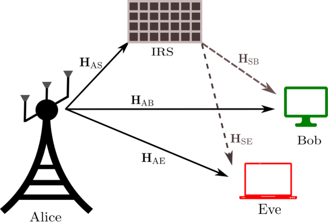
Consider an IRS-MIMOME system shown in Fig. 1, consisting of one transmitter (Alice), one legitimate receiver (Bob), and one eavesdropper (Eve). The number of antennas at Alice, Bob, and Eve are denoted by , , and , respectively, and the IRS is assumed to be manufactured with low-cost passive reflecting elements. The complex-valued channel matrices for the Alice-IRS, IRS-Bob, IRS-Eve, Alice-Bob and Alice-Eve links are denoted by , , , , and , respectively. Following the arguments in [2, 3, 5, 6, 9, 10, 11, 12, 14], it is assumed that all these channel matrices are quasi-static and perfectly known at all of the nodes.11 1 The results in this paper serve as theoretical performance upper bounds for the IRS-MIMOME system with imperfect channel state information in practice.
The received signals at Bob and Eve are, respectively, expressed as
| (1) | ||||
where is the transmitted signal vector from Alice (intended for Bob); and are the additive white Gaussian noise (AWGN) at Bob and Eve, respectively. For ease of presentation, in the rest of the paper we assume , where is noise power spectral density and is the signal bandwidth. With a slight abuse of notation and without loss of generality, in the sequel of the paper, we normalize the involving channels appropriately with the noise power, i.e., we define , , , and , and thus the resulting equivalent noise has a unit variance. In (1), , where , , , and denotes the phase shift induced by the -th reflecting element at the IRS.22 2 Although various models for IRS phase-shifts have been introduced recently [15], the unit-modulus model is the most frequently used in literature [2, 3, 5, 6, 9, 10, 11, 12, 14] for research investigation.
II-B Problem Formulation
Denoting the transmit covariance matrix at Alice by , the achievable secrecy rate (in nats/s/Hz) between Alice and Bob is given by
| (2) |
where , . On the other hand, the total power consumption to achieve the secrecy rate given in (2) is expressed as (c.f. [3])
| (3) |
where , , and are the constant circuit power consumption at Alice, IRS and Bob, respectively, and is the power amplifier efficiency at Alice. Following the arguments in [3], the power consumption at the IRS is modeled as , where is the circuit power consumption at each of the reflecting element in the IRS. Note that in (3), we do not consider the circuit power consumption at Eve. Such a scenario is justified where Eve is a node external to the main system. Then the SEE (in nats/s/Joule) for the IRS-MIMOME system can be defined as
| (4) |
where is the total available bandwidth and is the SEE in nats/s/Hz/Joule. In this paper, our objective is to maximize the SEE of the IRS-MIMOME system, the corresponding optimization problem can be formulated as follows:
| (5a) | ||||
| (5b) | ||||
| (5c) | ||||
| (5d) | ||||
where is the maximum transmit power budget at Alice, and is the threshold secrecy rate to maintain a minimum required quality of service (QoS) at Bob. Note that is the SEE of the system under consideration, the constraint in (5b) ensures the secrecy QoS at Bob, and those in (5c) and (5d) refer to the transmit power constraint at Alice and unit-modulus constraints at the IRS, respectively. We further define the feasible set for the optimization variables and as and , respectively.
III Proposed Solution
III-A Algorithm Description
It can be observed that the problem in (5) is non-convex due to the coupling of and in both (5a) and (5b), and the non-convexity of the constraints in (5d). In order to solve a similar optimization problem for a system consisting of a multi-antenna Alice, one single-antenna Bob, multiple single-antenna Eve, and one multi-antenna friendly jammer, the authors in [13] proposed an AO-based algorithm using SDP and Dinkelbach’s method. It is important to note that due to the existing coupling of the optimization variables in both objective function and optimization constraints, the proposed AO-based algorithm in [13] cannot guarantee a stationary solution to the optimization problem involving the use of Gaussian randomization to recover the rank-one matrix, and thus normally results in an inferior system performance. Furthermore, the complexity of the proposed solution in [13] is excessively high due to the use of SDP. Motivated by these drawbacks, in this paper, we propose a low-complexity PDDAPG method to find a stationary solution to (5). A similar method was recently shown to be effective for the achievable rate maximization problem in an IRS-assisted MIMO underlay spectrum sharing system in [14].
In order to deal with the non-convex coupling constraint in (5b), we adopt the penalty dual decomposition method [16]. For this purpose, we define . It is straightforward to note that for some , (5b) is equivalent to . Following the arguments in [16], for a given Lagrangian multiplier and a penalty parameter , an augmented Lagrangian function corresponding to (5a) can be defined as follows:
| (6) |
Therefore, for fixed and , we arrive at the following equivalent optimization problem:
| (7a) | ||||
| (7b) | ||||
It is noteworthy that the coupling of and is now included in the augmented objective and the constraints are decoupled in (7). Therefore, to obtain a stationary solution to (7), we apply a simple, yet efficient, numerical technique based on alternating gradient projection (APG) method.33 3 Following the arguments in [16], it can be shown that a stationary solution to (7) is indeed a stationary solution to the original problem in (5) at the convergence. For this purpose, we first find as follows:
| (8) |
Using (8) and [17, eqns. (6.207), (6.195) and Table 4.3], a closed-form expression for is given by (9), shown at the top of the next page. On the other hand, using [2, eqn. (17a)] and [17, Table 4.3 and eqn. (6.153)], a closed-form expression for is given by (10), shown at the top of the next page.
| (9) |
| (10) |
The gradient projection algorithm to solve (7) for fixed and is given in Algorithm 1, where and are the step size corresponding to and , respectively. Moreover, in line 3, for a given , its projection onto the set , i.e., can be shown to admit a water-filling solution. On the other hand, in line 4, for a given , its projection onto the set , i.e., is given by , where
| (11) |
Note that (11) ensures , and when , is chose randomly from the interval . After updating and in Algorithm 1, we update in line 6. Appropriate values of and in each iteration can be obtained using a backtracking line search routine as suggested in [2, Sec. IV-C]. Once the convergence is achieved in Algorithm 1, we update the Lagrange multiplier and the penalty parameter . The overall description of the proposed PDDAGP method to find a stationary solution to (7) is outlined in Algorithm 2. The convergence of Algorithm 2 can be proved following the similar line of arguments as provided in [14, Sec. III-C].
III-B Complexity Analysis
In this subsection, we present the complexity analysis of our proposed PDDAGP method. In this context, we use notation to present the per-iteration complexity of Algorithm 2, where we count the total number of required complex-valued multiplications. It is important to note that the per-iteration complexity of Algorithm 2 is dominated by that of the Algorithm 1.
We first calculate the complexity of computing (line 3) in Algorithm 1. For this purpose we need to compute .whose computational complexity is given by . The complexity for obtaining an appropriate value of and projecting onto results in an additional complexity of .
Next, we calculate the complexity associated with the computation of (line 4) in Algorithm 1. Note that the complexity associated with the computation of an appropriate and the projection of will be negligible as compared to that of computing , and therefore, the complexity of computing will be the same as that of , given by .
The complexity of computing (line 5) in Algorithm 1 is negligible compared to that of and . Therefore, the per-iteration complexity of the Algorithm Algorithm 2 is given by . We note that in a practical IRS-MIMOME system we should have . Therefore, the complexity of the proposed algorithm can be approximated by , meaning that the computational complexity of the proposed PDDAGP algorithm increases linearly with . We remark that for the IRS-assisted MISO WTC case, the complexity of the proposed algorithm is reduced to to , which is notably lower than that of the SDP-based algorithm proposed in [13] and the former is more suitable for practical implementation.
IV Numerical Analysis
In this section, we first describe the simulation parameters considered in this paper. The center of the Alice’s, Bob’s and Eve’s uniform linear array is assumed to be located at , , and , respectively. The center of the IRS is denoted by . The inter-antenna separation at Alice, Bob, and Eve, and the distance between any two of the neighboring reflecting elements at IRS is assumed to be equal to ; here denotes the wavelength of the carrier waves.
The Alice-Bob and Alice-Eve channels are defined as , , where the elements in given by corresponds to the line-of-sight (LoS) component, represents the non-line-of-sight (NLoS) component, denotes the distance between the -th antenna at the transmitter (Alice) and the -th antenna at the receiver (Bob/Eve), and is the Rician factor. Moreover, the elements in correspond to the free-space path loss (FSPL) coefficients and are given by . Similarly, the IRS-Bob and IRS-Eve links are modeled as . The elements in are given by , , the elements in are given by , is the distance between the -th reflecting element at the IRS and the -th antenna at Bob/Eve and is the antenna gain at Bob/Eve. The Alice-IRS channel is modeled as , where the elements in given by represent the FSPL coefficients, the elements in are given by , , is the distance between the -th antenna at Alice and the -th reflecting element at the IRS, and is the antenna gain at Alice.
Unless stated otherwise, in this section we consider , m, m, m, m, m, m, m, m, m, m, dBm, dBm/Hz, , MHz, , dBm and dBm. We performed the numerical experiments using the MATLAB (R2022a) on a 64-bit Windows machine with 16 GB RAM and an Intel Core i7 3.20 GHz processor. Note that in Fig. 4-7, the average rum time/average SEE is computed over 1000 independent channel realizations and the Fig. 4,4 are constructed based on single channel realization.
We now present the numerical results to evaluate the performance of the proposed method for the IRS-MIMOME system under consideration. In Fig. 4, we show the convergence results of Algorithm 2. It is evident from Fig. 4 that the augmented objective function and the original objective function converge to the same value, indicating that the regularized term becomes zeros at convergence, which is in-line with the theory of penalty-based optimization schemes. Note that for fixed and , we consider to be converged when the relative difference in , i.e., becomes less than or equal to the tolerance value . After this, we update the Lagrangian multiplier and the penalty parameter . Finally the algorithm is considered convergent when . We remark that Algorithm 2 aims to maximize the augmented objective function , and thus for fixed values of and , increases monotonically.
In Fig. 4 we compare the performance our proposed algorithm with that of [13, Algorithm 1]. It is important to note that since [13, Algorithm 1] is applicable only for IRS-MISOSE system, in Fig. 4 we consider . It is evident from the figure that both the proposed PDDAGP and [13, Algorithm 1] takes almost the same number of iterations to achieve the convergence, however, the proposed PDDAGP method attains a higher SEE. The main reason for the inferior performance of the method proposed in [13, Algorithm 1], which is based on AO, is its way in handling the coupling between the optimization variables in the constraint. It is well known that AO-based algorithms can be easily trapped in ineffective solution due to poor initialization. The involved Gaussian randomization is another reason for the inferior performance of [13, Algorithm 1]. Note that in the case of PDDAGP algorithm, the coupling in the constraint is brought to the objective in the form of a penalized term. This move makes optimization variables decoupled, which results in a superior performance as demonstrated.
We now numerically shown that the proposed algorithm also outperforms [13, Algorithm 1] in terms of the required runtime, which validates the complexity analysis presented in preceding section. To this end, in Fig. 4 we compare the average runtime of Algorithm 2 and [13, Algorithm 1] w.r.t. . It is clearly evident from the figure that the proposed PDDAGP algorithm takes significantly less time to converge on average compared to that for [13, Algorithm 1]. This is because the complexity of our proposed algorithm grows only linearly w.r.t. , where the complexity of SDP-assisted Dinkelbach’s method in [13, Algorithm 1] is excessively high.
In Fig. 7, we compare the average SEE performance versus for the proposed PDDAGP algorithm with that of a baseline scheme which we refer to as ZFrand. In this ZFrand scheme, for a fixed we find that maximizes (5) while satisfying (which is essentially the zero-forcing precoder) and (5b). Due to the ZF constraint, problem (5) can be reformulated as a convex program and thus can be found exactly. Then for a given , to update , we follow a procedure similar to Gaussian randomization, i.e., randomly many s and select the one that gives the best objective . It is noticeable that our proposed PDDAGP method outperforms the ZFrand scheme, which is expected because of the suboptimality of ZF beamformer and as well as that of selecting the random .
In Fig. 7, we show the impact of the number of reflecting elements at the IRS, i.e., . Note that increasing increases both and , resulting in a non-trivial trade-off for the SEE. In the figure, we consider different values for the circuit power consumption per IRS element, i.e., . It is observed from Fig. 7 that for a small value of , the IRS-MIMOME system can achieve a significantly higher SEE compared to its non-IRS counterpart. On the other hand, a large value of may result in a performance degradation in terms of average SEE in an IRS-MIMOME system compared to the non-IRS counterpart. Therefore, it can be concluded that for a given , there exists an optimal value of to maximize the benefit of using an IRS in terms of average SEE.
In Fig. 7, we compare the average SEE of the system under the consideration with its non-IRS counterpart, for two different scenarios: (i) optimal power allocation and optimal IRS phase-shifts (i.e., (5)), and (ii) full power allocation and optimal IRS phase-shifts (i.e., (5) with (5c) modified to ). We note that is the logarithmic function while is a linear function w.r.t. to . So, in the case of full power allocation, for small values of , the average SEE first increases with increasing values of because the rate of increase of is larger than that of the . However, for large values of , increases at a much faster rate compared to , resulting in a loss in SEE. On the other hand, for the case of optimal power allocation, the system uses full power () for small values of , however, it uses a smaller transmit power than the maximum available for large value of . Specifically, for the case of optimal power allocation in the large regime, becomes strictly less than , irrespective of the value of which results in a constant value of both and . This in turn results in a saturated value of SEE, i.e., for increasing value of .
V Conclusion
In this paper, we considered the problem of the SEE maximization in an IRS-MIMOME system, subject to a transmit power constraint (at the transmitter), a target secrecy rate constraint (at the legitimate receiver), and unit-modulus constraints at the IRS. We proposed a PDDAGP method to find a stationary solution to the challenging non-convex optimization problem of the SEE maximization. Extensive numerical experiments were performed to evaluate the performance of the proposed algorithm, and the superiority of the PDDAGP method was also established over that of an SDP-assisted Dinkelbach’s method for the special case of IRS-MISOSE system. We also showed that the per-iteration complexity of the proposed PDDAGP method grows as linearly w.r.t. the number of reflecting elements at the IRS, that is appealing for practical implementation.
References
- [1] S. Basharat, S. A. Hassan, H. Pervaiz, A. Mahmood, Z. Ding, and M. Gidlund, “Reconfigurable intelligent surfaces: Potentials, applications, and challenges for 6G wireless networks,” IEEE Wireless Commun., vol. 28, no. 6, pp. 184–191, Dec. 2021.
- [2] N. S. Perovic, L.-N. Tran, M. Di Renzo, and M. F. Flanagan, “Achievable rate optimization for MIMO systems with reconfigurable intelligent surfaces,” IEEE Trans. Wireless Commun., vol. 20, no. 6, pp. 3865–3882, Feb. 2021.
- [3] C. Huang, A. Zappone, G. C. Alexandropoulos, M. Debbah, and C. Yuen, “Reconfigurable intelligent surfaces for energy efficiency in wireless communication,” IEEE Trans. Wireless Commun., vol. 18, no. 8, pp. 4157–4170, Jun. 2019.
- [4] X. Chen, D. W. K. Ng, W. H. Gerstacker, and H.-H. Chen, “A survey on multiple-antenna techniques for physical layer security,” IEEE Commun. Surveys Tuts., vol. 19, no. 2, pp. 1027–1053, 2017.
- [5] A. Mukherjee, V. Kumar, and L.-N. Tran, “Secrecy rate maximization for intelligent reflecting surface assisted MIMOME wiretap channels,” in IEEE MILCOM, Nov. 2021, pp. 261–266.
- [6] V. Kumar, M. F. Flanagan, D. W. Kwan Ng, and L.-N. Tran, “On the secrecy rate under statistical QoS provisioning for RIS-assisted MISO wiretap channel,” in IEEE GLOBECOM, Feb. 2021, pp. 1–6.
- [7] J. Xu and L. Qiu, “Energy efficiency optimization for MIMO broadcast channels,” IEEE Trans. Wireless Commun., vol. 12, no. 2, pp. 690–701, Jan. 2013.
- [8] K. N. R. S. V. Prasad, E. Hossain, and V. K. Bhargava, “Energy efficiency in massive MIMO-based 5G networks: Opportunities and challenges,” IEEE Wireless Commun., vol. 24, no. 3, pp. 86–94, Jun. 2017.
- [9] S. Jia, X. Yuan, and Y.-C. Liang, “Reconfigurable intelligent surfaces for energy efficiency in D2D communication network,” IEEE Wireless Commun. Lett., vol. 10, no. 3, pp. 683–687, Mar. 2021.
- [10] S. Zargari, A. Khalili, and R. Zhang, “Energy efficiency maximization via joint active and passive beamforming design for multiuser MISO IRS-aided SWIPT,” IEEE Wireless Commun. Lett., vol. 10, no. 3, pp. 557–561, Mar. 2021.
- [11] Z. Yang et al., “Energy-efficient wireless communications with distributed reconfigurable intelligent surfaces,” IEEE Trans. Wireless Commun., vol. 21, no. 1, pp. 665–679, Jul. 2021.
- [12] X. Wu, J. Ma, Z. Xing, C. Gu, X. Xue, and X. Zeng, “Secure and energy efficient transmission for IRS-assisted cognitive radio networks,” IEEE Trans. Cogn. Commun. Netw., vol. 8, no. 1, pp. 170–185, Sep. 2021.
- [13] Q. Wang, F. Zhou, R. Q. Hu, and Y. Qian, “Energy efficient robust beamforming and cooperative jamming design for IRS-assisted MISO networks,” IEEE Trans. Wireless Commun., vol. 20, no. 4, pp. 2592–2607, Dec. 2021.
- [14] V. Kumar, M. Flanagan, R. Zhang, and L.-N. Tran, “Achievable rate maximization for underlay spectrum sharing MIMO system with intelligent reflecting surface,” IEEE Wireless Commun. Lett., vol. 11, no. 8, pp. 1758–1762, 2022.
- [15] B. Feng et al., “Optimization techniques in reconfigurable intelligent surface aided networks,” IEEE Wireless Commun., vol. 28, no. 6, pp. 87–93, Dec. 2021.
- [16] Q. Shi and M. Hong, “Penalty dual decomposition method for nonsmooth nonconvex optimization–Part I: Algorithms and convergence analysis,” IEEE Trans. Signal Process., vol. 68, pp. 4108–4122, Jul. 2020.
- [17] A. Hjørungnes, Complex-valued matrix derivatives: With applications in signal processing and communications. Cambridge University Press, 2011.