Quantum Mixed State Compiling
Abstract
The task of learning a quantum circuit to prepare a given mixed state is a fundamental quantum subroutine. We present a variational quantum algorithm (VQA) to learn mixed states which is suitable for near-term hardware. Our algorithm represents a generalization of previous VQAs that aimed at learning preparation circuits for pure states. We consider two different ansätze for compiling the target state; the first is based on learning a purification of the state and the second on representing it as a convex combination of pure states. In both cases, the resources required to store and manipulate the compiled state grow with the rank of the approximation. Thus, by learning a lower rank approximation of the target state, our algorithm provides a means of compressing a state for more efficient processing. As a byproduct of our algorithm, one effectively learns the principal components of the target state, and hence our algorithm further provides a new method for principal component analysis. We investigate the efficacy of our algorithm through extensive numerical implementations, showing that typical random states and thermal states of many body systems may be learnt this way. Additionally, we demonstrate on quantum hardware how our algorithm can be used to study hardware noise-induced states.
I Introduction
The task of learning an unknown quantum state is a fundamental primitive for quantum computing. The well known method of full quantum state tomography learns the matrix elements of directly. The original scheme employs Pauli measurements to learn the state up to additive error in trace distance Nielsen and Chuang 2000. Subsequent refinements require only measurements Haah et al. 2017, or allowing for a small failure probability O’Donnell and Wright 2016. A recent improvement has found it is necessary to use at least measurements, and it was also conjectured to be sufficient Yuen 2022. In all cases, tomography aims to obtain a classical description of a quantum state, and as such, the number of measurements it requires scales exponentially with the number of qubits of the target state.
An alternative approach is to give a more operational meaning to learning. In practice, we are often not interested in the exact form of but instead in its properties; i.e., we wish to estimate for some observable . Ref. Aaronson 2019 proves that if each observable , for , is restricted to two-outcome measurements, then only copies of are sufficient to estimate each up to additive error by using a method called shadow tomography Huang et al. 2020; Elben et al. 2022; Huang et al. 2022. These results were expanded to simpler, experimentally tractable Clifford measurements and random Pauli measurements in Refs. Huang et al. 2020; Paini et al. 2021. In particular, it was shown that a polynomial number of Clifford (Pauli) measurements is sufficient to estimate any low rank (local) observable. The polynomial scaling achieved by shadow tomography is gained at the cost of providing only a partial description of the quantum state.
Yet another approach to quantum state learning, and the one we take here, is instead to solve the problem of state compilation. This involves learning a quantum circuit with which we may prepare an approximation of the target state. In this paper, we propose and demonstrate a near-term algorithm for approximately compiling an unknown quantum state by variationally training a parameterized quantum circuit. Similar to the shadow tomography case, one can use the final cost function value in our algorithm to place bounds on the deviation of observables estimated from the learnt state from those of the target state.
While the variational compilation of pure states has been explored in Refs. Khatri et al. 2019; Jones and Benjamin 2022; Sharma et al. 2020, here we focus on mixed state compilation. Specifically, we propose two different ansätze that can compile a mixed state either into a purification using ancilla or as a convex combination of pure states. The latter is similar to the Hamiltonian-based model approach in Ref. Verdon et al. 2019. In addition, our approach shares similarities with Refs. LaRose et al. 2019; Cerezo et al. 2022, which present algorithms to learn the diagonalization of a target state, but in contrast to our approach, these methods only apply to low-rank quantum states.
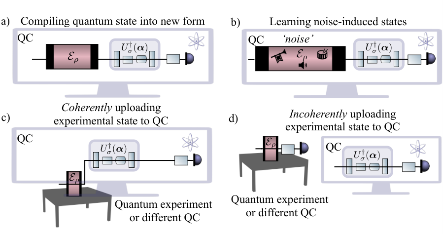
Quantum state compilation, in providing a quantum circuit description of a state, serves a different purpose from tomography or classical shadows, as summarized in Fig. 1. In the first case, it may be used to ‘upload’ an unknown state of an experimental quantum system to a quantum computer. In other words, given a quantum system in an unknown target mixed state, our algorithms can learn a circuit representation of it for implementation on any digital quantum device. In this case, we can use the compilation to more efficiently store the state for later processing, compute properties of the state that are hard to measure directly, or use the state as the input to another algorithm, say for quantum simulation. Alternatively, a circuit to prepare the target state might already be known, but the aim would be to learn a more efficient (i.e., shorter depth and/or more noise resilient) circuit to prepare that state. These applications are particularly interesting when the unknown mixed state is generated by unknown noise as in (b). In this case, the compilation serves as a snapshot of how a noisy quantum computer corrupted a desired input state. This snapshot can then be used later or perhaps even on a more coherent machine for reliable processing.
In some cases, it may be of interest not to learn the target state perfectly but rather attempt to learn a low(er) rank approximation of it. In general, the resources required to manipulate a quantum state on quantum hardware grow with its rank. Thus, learning a lower rank approximation provides a means of compressing a state to store it more efficiently. The compression of quantum data has a long history tracing back to the early days of quantum information theory Schumacher 1995; Cleve and DiVincenzo 1996; Nielsen and Chuang 2000. More recently, the question of how well any given state may be approximated using a lower rank state was addressed analytically in Ref. Ezzell et al. 2022 for the Hilbert–Schmidt and trace distances. Interestingly, the optimal lower rank approximation essentially corresponds to performing principal component analysis (PCA) (jump to Eq. (3) to look ahead) for the Hilbert–Schmidt distance (but not for trace distance). Hence, as we will show, one can also use our learned compilation to perform PCA with a desired cut-off rank. At the same time, the analytical expression for the optimal state from this work provides a natural benchmark for our learning task.
Our algorithm, which is summarized in Fig. 2, involves variationally minimizing a cost function that is formulated in terms of the Hilbert–Schmidt distance between the target state and ansatz state. This cost can be efficiently measured using either a SWAP test or a Loschmidt echo circuit. In contrast to Ref. Lloyd and Weedbrook 2018, which sketches a quantum generative adversarial neural network that might be used to learn a mixed state, we further present local variants of our cost functions to mitigate the trainability barrier posed by barren plateaus McClean et al. 2018; Cerezo et al. 2021; Holmes et al. 2021a; Holmes et al. 2022; Arrasmith et al. 2022; Larocca et al. 2022a; Sharma et al. 2022; Patti et al. 2021; Thanasilp et al. 2021; Uvarov and Biamonte 2021; Marrero et al. 2021.
In the numerical simulations of our proposed algorithm, we demonstrate the applicability of both the purification and convex combination ansätze for learning full and lower rank approximations of a target mixed state. In particular, we numerically simulate the learning of typical random states, as well as of random thermal states of the Heisenberg XY model. We additionally implement our algorithm on quantum hardware in order to compile an unknown state generated by hardware noise.

II Quantum Mixed State Compiling Algorithm
The Quantum Mixed State Compiling (QMSC) algorithm takes as input a mixed state and a desired approximation rank . Though not necessary, we assume in defining our algorithm since this is both sensible and simplifies our discussion. In our algorithm, we take this a step further and constrain , where is the -rank11 1 We note that the notion of -rank was also used in Ref. Cerezo et al. 2020, but its formal definition is slightly different than the one we choose to use here. A smooth version of the max-entropy (or Renyi entropy) provides yet another definition for -rank that is distinct from ours Renner and Wolf 2004; Renner 2005. of , which counts the number of eigenvalues greater than . This notion of approximate rank is designed to capture the intuition that the contribution of very small but non-zero eigenvalues can often in practice be ignored. The goal then is to optimize the classical parameters of a parameterized trial state satisfying , such that, for the optimized parameters , the output state well approximates the target .
In order to assess the closeness between our training state and our target state , we employ the following cost function in terms of the Hilbert–Schmidt distance between the two states:
| (1) | ||||
As discussed in more detail in Sections II.3 and II.4, the Hilbert–Schmidt distance can be efficiently computed using a combination of SWAP tests and/or a Loschmidt-echo-like circuit. In Appendix A we detail how this cost can be reformulated such that it requires only local measurements Cerezo et al. 2021 to mitigate the barrier to trainability posed by barren plateaus McClean et al. 2018; Cerezo et al. 2021; Holmes et al. 2021a; Holmes et al. 2022; Arrasmith et al. 2022; Larocca et al. 2022a; Sharma et al. 2022; Patti et al. 2021; Thanasilp et al. 2021; Uvarov and Biamonte 2021; Marrero et al. 2021.
If trained well, the learned state should be close to the solution to the Quantum Low-Rank Approximation Problem Ezzell et al. 2022. As discussed in Ref. Ezzell et al. 2022, the unique optimal state that minimizes the Hilbert–Schmidt distance, subject to a rank constraint, i.e., the state where
| (2) |
takes the form
| (3) | ||||
| (4) |
Here is a projector onto the eigenstates corresponding to the largest eigenvalues of . That is, is a projector onto the first principal components of . We note here that the projection is the same conceptually as the typical subspace projection (Ohya and Petz 2004, page 31, Theorem 1.18) used in quantum data compression Schumacher 1995 (given that it projects onto the high probability subspace of the state ), and the quantum channel in (3) (i.e., ) is essentially the same as the encoding channel used in quantum data compression (Nielsen and Chuang 2000, equation (12.50)).
With this analytical solution, we can define a natural performance metric for the Quantum Mixed State Compilation algorithm as the difference between the found cost and optimal possible cost,
| (5) |
More explicitly, this expression takes the form
| (6) |
where denotes the set of eigenvalues of the target state. Of course when is truly unknown, we can only report the optimal cost , but in this work, we actually compute to verify that our algorithm is working as intended.
In this paper, we develop a practical, noisy intermediate-scale quantum (NISQ)-friendly algorithm to find , an approximation of . In doing so, we also find the first principal values and components of , and so we are essentially performing quantum principal component analysis (PCA), analogous to some previously proposed algorithms Lloyd et al. 2014; LaRose et al. 2019; Cerezo et al. 2022. The precise form in which (or the first principal components) is obtained depends on our choice of ansatz. We consider two different ansätze, one based on learning an approximate purification of and the second on decomposing an approximation of it into a convex combination of pure states. We also discuss the complexity of computing our cost function, as well as its operational meaning. These are detailed in the following sections. A summary of our algorithm, which also describes the two ansätze choices, is given in Fig. 2.
II.1 Complexity of Cost Function
For all VQAs, the purpose of using the quantum computer in the optimization loop is to estimate a cost function efficiently, which otherwise would be difficult to estimate classically. Hence, it is helpful to establish that the cost function is indeed classically hard to estimate. Previously proposed VQAs for quantum compiling Khatri et al. 2019 and linear system solving Bravo-Prieto et al. 2019 have established classical hardness via the DQC1 hardness of estimating the relevant cost function. (In the previous sentence, DQC1 stands for deterministic quantum computation with one clean qubit Knill and Laflamme 1998). We can make this same argument for the cost function in Eq. (1), as follows.
A special case of computing Eq. (1) is when the two states happen to be Choi states associated with unitary processes acting on a dimensional Hilbert space. In this case, we write and , where , , and is the standard Bell state. Then the cost function in (1) becomes where . Hence, in this special case we have that where is the Hilbert–Schmidt test cost of Ref. Khatri et al. 2019. Estimating the latter was shown to be DQC1-hard in Ref. Khatri et al. 2019, and hence our cost function is also DQC1-hard. Since efficient classical simulation of DQC1 would imply a collapse of the polynomial hierarchy Fujii et al. 2018; Morimae 2017, standard complexity assumptions imply the classical hardness of estimating .
II.2 Operational Meaning of Cost Function
II.2.1 Observable estimation
There is a close connection between the Hilbert–Schmidt distance and trace distance for low-rank states Coles et al. 2019, which gives operational meaning to our cost function in this case. Namely when at least one of the states is low rank, then the two distance measures are essentially equivalent Coles et al. 2019. This can be seen from the following inequality relating the 2-norm to the 1-norm:
| (7) |
for any two density matrices and . Here, is a quantity called the reduced rank, which is analogous to the reduced mass employed in physics.
In this sense, one can use the Hilbert–Schmidt distance, and hence our cost function, as a strong upper bound on the trace distance. In turn, the trace distance has operational meaning in terms of the difference of observable expectation values on the two states Nielsen and Chuang 2000, where the maximization is over all POVM (Positive Operator Valued Measure) elements , i.e., operators satisfying . Hence, our cost function inherits this operational meaning:
| (8) |
for any POVM element , where is the reduced rank for and .
II.2.2 Eigenvalue and Eigenvector Estimation
We also establish an operational meaning for our cost function in the context of minimizing the errors in the eigenvectors and eigenvalues of the compiled state. This is particularly relevant in the context of using our algorithm for PCA, since PCA precisely aims to extract the eigenvectors with the largest eigenvalues.
First, we note that our proposed cost is an upper bound on the squared difference between the true eigenvalues of and the eigenvalues of the learnt state , as follows. Let us denote the eigenvalues of in increasing order as and the eigenvalues of as , with the Hilbert space dimension. Then a measure of eigenvalue error is
| (9) |
It then follows from the Hoffman–Wielandt theorem that
| (10) |
Thus if one can achieve a small cost value, the average error in the learnt eigenvalues is guaranteed to be small.
We remark that a small cost value might not be achievable since the optimal cost is often non-zero. In this case, one could consider an alternative measure of eigenvalue error that, unlike (9), would vanish for the optimal state in (3). Namely, one can consider the set of states that have the correct -largest eigenvalues up to an additive constant, and then define a measure of eigenvalue error as . Then it is clear that our cost function upper bounds this error as well: .
Second, we note that our proposed cost function is an upper bound on the eigenvector error measure introduced in Ref. LaRose et al. 2019. Specifically, a natural measure of the difference between the true eigenvectors of the target state, , and the learnt eigenvectors, , is given by
| (11) |
where
| (12) |
Expanding this out we have that
| (13) |
where for the inequality we use the fact that
| (14) |
(i.e., the trace can be taken with respect to an arbitrary orthonormal basis). Thus a small cost function guarantees a small eigenvector error by this measure.
II.3 State Purification Ansatz
Let us now move onto the different types of ansatz constructions. The state purification (SP) ansatz constructs trial states of the form
| (15) |
where acts on the system qubits (the same qubits where the state resides) plus an ancilla register composed of qubits. In using ancillas, we guarantee that , but for a typical parameterized circuit with randomly generated parameters, one has precisely . Thus, in practise, the SP ansatz is only compatible with controlling in powers of two, so that . While there are many different possible choices in the ansatz for , we suggest using either a problem-inspired approach obeying the symmetries of the target state Gard et al. 2020; Gibbs et al. 2021; Larocca et al. 2022b and/or an adaptive approach Bilkis et al. 2021 to mitigate the problem posed by barren plateaus. A discussion of specific choices in our work for different ensembles is given in Appendix B.
Upon substitution of the SP ansatz into our proposed Hilbert–Schmidt distance-based cost function, we obtain
| (16) |
where we use to denote the system of the states and . Below we describe efficient ways of computing each of these terms.
Purity of target
The purity of the target may be measured using a SWAP test Barenco et al. 1997 or its destructive variant Garcia-Escartin and Chamorro-Posada 2013. For the estimate to be within additive error of the true value with probability not smaller than , the Hoeffding bound implies that it suffices to take samples. Alternatively, as this term remains constant throughout the procedure, we may opt to neglect it and only focus on optimizing the remaining two parameter-dependent terms.
Purity of ansatz
The purity of the ansatz may again be measured via a SWAP test. It is also possible to make use of the fact that we are representing it via its purification and measure the purity of the ansatz via the Loschmidt-echo circuit shown in Fig. 2. Again, from the Hoeffding bound, it suffices to take samples.
Overlap term
The overlap term can be evaluated using either a SWAP test or the Loschmidt-echo type circuit pictured in Fig. 2. The latter requires fewer qubits and controlled unitaries and hence is more NISQ friendly. To see why this circuit works, note that since we prepare the trial state via a higher-dimensional purification found by evolving an initial all-zero state to the purification of , we can rewrite the overlap term as follows
| (17) | ||||
This corresponds to preparing a maximally mixed state on the qubit ancillary system alongside which is prepared on the system register , evolving the system and ancilla registers under , and then performing an all-zero measurement. Due to the factor of , the number of shots required to measure this cost within additive error will scale exponentially in the number of ancilla qubits . Hence the Loschmidt echo method for computing the overlap is only appropriate for learning low rank approximations to where .
As discussed earlier, the above method may also be used to calculate the purity of our ansatz simply by replacing the initial state with the trial state . However, the purity of our target may not be measured this way, as it requires knowledge of a purification of , which is precisely what we are trying to find.
II.4 Convex Combination of Pure States Ansatz
The convex combination of pure states (CCPS) ansatz constructs trial states of the form
| (18) |
Here denotes a subset of the computational basis of qubits, is a vector of parameters, is a parameterized quantum circuit, and is a parameterized probability distribution. An appealing feature of this ansatz is that learning a rank- approximation gives any rank approximation for free since one can always ‘drop’ the eigenstates corresponding to the smallest eigenvalues and then re-normalize (see Eq. (31a)).
Since the state that minimizes our cost, (i.e., the solution to the Quantum Low-Rank Approximation Problem given in Eq. (3)), is proportional to the first principal components of the target state , it follows that this ansatz can be used to learn the principal components of . More precisely, we have that the first principal values of are given by and its principal components are .
When the rank of the trial state is low, i.e., , such that we are learning a low rank approximation of the target state , or for small scale problems, the vector of probabilities may be stored simply as a classical vector. For learning high rank approximations to larger full rank states, the probability vector is exponentially large and thus cannot be explicitly stored efficiently. Rather the process will need to be sampled from. Such samples can be generated via classical neural networks, such as generative neural networks Yang 2022 or Boltzmann machines Montúfar 2016. In this case, there are similarities between the CCPS ansatz and the Hamiltonian models considered in Ref. Verdon et al. 2019. Similarly to the SPA, for we suggest using either a problem inspired ansatz obeying the symmetries of the target state Gard et al. 2020; Gibbs et al. 2021; Larocca et al. 2022b and/or an adaptive approach Bilkis et al. 2021. A discussion of specific choices in our work for different ensembles is given in Appendix B.
Upon substituting the expression for the convex combination of pure states ansatz into our proposed Hilbert–Schmidt distance cost function, we obtain
| (19) |
with . Here we describe how each of the terms in the above cost may be efficiently computed.
Purity of target.
As for the state purification ansatz, the first term, i.e., the purity of the target state, may be computed using a SWAP test Barenco et al. 1997 or its destructive variant Garcia-Escartin and Chamorro-Posada 2013 (see also Ref. Subaşı et al. 2019).
Purity of ansatz.
The second term, the purity of the guessed state, is equal to the sum of the square of the probabilities of the parameterized distribution, . For low rank approximations, i.e., , one may store the probability vector classically and thus this term can be computed by basic arithmetic.
When the probability vector is too large to be stored explicitly, but rather is handled via sampling, the purity of the ansatz can be estimated with a classical version of the SWAP test. Indeed, the approach is to take two independent samples from the distribution (call the random samples and ). We then set an indicator random variable as if the samples are not equal, and if the samples are equal. The expectation of this random variable is then given by
| (20) | ||||
| (21) | ||||
| (22) | ||||
| (23) |
Thus, the random variable is an unbiased estimator of the collision probability, , and takes values between zero and one. The Hoeffding bound then applies, and we can take independent samples of in order to estimate the collision probability to within additive error with probability not smaller than .
Overlap term.
A naive approach to computing the third term, the overlap between the guess and target , would be to estimate each of the terms using the Loschmidt echo circuit shown in Fig. 2, followed by classical post processing. That is, we compute by preparing the state , performing the unitary , and then measuring in the computational basis. The total overlap term could simply be computed by weighting each of the probabilities by the corresponding classical probability and taking their sum. This naive approach will work for small problems; however, even in the case where can be explicitly stored, this method will not be efficient for larger problems. The problem is that one needs enough shots to estimate all probabilities . Combining this observation with Hoeffding’s equality, it is apparent that this method requires an exponential number of shots, .
Instead, we propose computing the overlap term using a generalization of the classical SWAP test. Let us define the distribution
| (24) |
which can be sampled from via the Loschmidt echo circuit. Then we see that
| (25) |
This quantity can be estimated by taking a sample from and an independent sample from (call the samples and ) and setting an indicator random variable if the samples are not equal and if the samples are equal. The expectation of this random variable is given by
| (26) | ||||
| (27) | ||||
| (28) | ||||
| (29) |
Thus, the random variable is an unbiased estimator of the collision probability , and it takes values between zero and one. The Hoeffding bound then applies, and we can take independent samples of in order to estimate this collision probability to within additive error with probability not smaller than .
II.5 Performing PCA with our Ansätze
Both ansätze also allow for principal component analysis (PCA) of . To make this precise, we first write the target state as
| (30) |
where are the ordered principal values of with associated principal components .
By inspection, the CCPS ansatz is directly an ansatz for the principal components of . In other words, learning a CCPS representation of provides an estimate of the principal components, , explicitly. It also provides an estimate of the principal values, , but due to normalization, these are expected to be different from by an additive constant when is small. As approaches , this additive constant goes to zero, and here . Nevertheless, even when , the values of are such that acts as the closest rank proxy, so in this operational sense, it is still appropriate to call the principal value estimates.
One very useful property of these explicit principal component/value estimates is that they allow us to construct any numerically optimal approximation by truncation,
| (31a) | ||||
| (31b) | ||||
Indeed, this is perhaps one convincing way to view each as the appropriate operational sense of “principal value” when we truncate the rank.
Though less obvious, the SP ansatz can also be used for PCA by using a carefully designed circuit for the purification ansatz as described in Appendix B. The result is that computational basis measurements on the ancilla system prepare the principal vectors on the target system with probabilities given by the principal values. Thus, the knowledge of principal values/components here is implicit, and hence cannot be directly used to obtain lower rank approximations by truncation.
Finally, we remark that while PCA is a general procedure, it has an intuitive meaning for physically relevant classes of states. As an example, consider an XY thermal state. In general, the eigenvalues follow a Boltzmann distribution, and the eigenvectors are those of the XY Hamiltonian itself. At low temperature, we often say a state is approximately in its ground-state. More precisely, we mean,
| (32) |
for small. In our language, we would say the state is approximately rank , and when as is typical for low temperature thermal states, it’s approximately low rank 22 2 We comment that this exact notion of low rank actually precisely agrees with the definition of epsilon-rank used in Ref. Cerezo et al. 2020. We employ a slightly different definition already given that is more amenable to NISQ experiments.. By performing PCA with a target rank , we find approximations of the eigenvectors with low energies and corresponding Boltzmann weights . Hence, our PCA algorithm can be thought of as a way to learn the Boltzmann weights and a means to prepare low-lying energy eigenvectors of a quantum thermal state which has also been explored in other NISQ friendly works Guo et al. 2023.
II.6 Comparison of Ansätze
The reliance on an ancillary system to compute the cost function for the SP ansatz naturally increases the resources required for computation. Furthermore, in general, for a typical choice of , the guess state will have rank . That is, one is limited to ranks of powers of two. In contrast, CCPS both requires no ancilla and allows for fine control over both output ranks. However, the need to learn under the constraint of convexity, in addition to , potentially increases the complexity of our optimization subroutine. Thus the choice as to whether to use CCPS or SP will depend in large part on whether classical resources (optimization power) or quantum resources (qubits available) are more constrained.
Of course, the choice as to whether to use the CCPS or SP ansatz may depend not only on the required resources but also the end goal of the subroutine. For example, if the end goal is principal component analysis, this is more readily performed using CCPS since it automatically finds the first principal components of the target. Alternatively, one can imagine situations where it is desirable to learn the purification of the target. For example, the purification of a state opens up methods for computing entanglement measures between subsystems of that state Vedral and Plenio 1998; Schumacher 1996; Wilde 2013, the fidelity between two states (given Ulhmann’s theorem) Chen et al. 2021; Rethinasamy et al. 2021, as well as symmetry measures LaBorde and Wilde 2021.
II.7 Summary of Algorithm
The Quantum Mixed State Compiling algorithm is summarized in Fig. 2. At its core it is composed of the following steps.
- 1.
Start with a target state , and a desired rank for the compiled state used to approximate .
- 2.
Choose whether to learn the target using the purification or convex combination ansatz. In general, this decision will depend on the purpose for which the state is being learned and the resources available. A discussion of the circuits one must run in both cases is given in Appendix B.
- 3.
Minimize the Hilbert–Schmidt distance cost , Eq. (1), using a hybrid quantum-classical optimization loop to find the trained parameters (in the case of the SP ansatz) and (in the case of the CCPS ansatz) that approximately minimize . If using a gradient based optimizer one can analytically compute the gradient of the cost using the parameter shift rule Mitarai et al. 2018; Schuld et al. 2019. For the case of the purity of the ansatz term for the state purification ansatz, , this rule needs modifying to account for correlations. For more details on computing the gradients, see Appendix C.
Here we briefly describe two ways in which prior information about the structure of the target state could be used to make the mixed state learning algorithm more efficient.
In the first instance, the purity of the target state may be computed and then we need only consider ‘guess’ states with the correct purity. That is, one may use the target purity as a constraint during the minimization of the Hilbert–Schmidt distance cost, Eq. (1). This amounts to maximizing the overlap term subject to the constraint . We note that this constrained optimization may not be compatible with the rank constraint if the desired rank is much lower than the true rank of the target, i.e., .
Going a step further, one could also simplify the task of learning a rank- approximation to by first learning the largest eigenvalues of and then using the mixed state learning algorithm to learn their corresponding eigenvectors. The largest eigenvalues of any state can be learnt non-variationally using the quantum algorithm proposed in Ref. Subaşı et al. 2019. Denoting the measured eigenvalues as , the eigenvectors may be learnt by maximizing the overlap term .
As discussed further in Appendix A, one theoretical advantage of these two modifications is that they require optimizing only a single overlap term rather than the difference between two purity terms and an overlap term. This overlap term takes the form of a standard Variational Quantum Eigensolver (VQE) cost and therefore can be readily transformed into a local cost for which we have trainability guarantees Cerezo et al. 2021.
III Numerical Simulations
We begin our numerical simulations discussion with a brief summary of the target states and chosen optimizer. Additional details can be found in our open source code Ezzell 2022 which includes our raw data and the scripts we used to generate it. We then discuss the results of compiling each of the listed states in separate sections.
III.1 Description of States and Optimizer
We discuss the performance of our QMSC algorithm for three main types of states:
- 1.
Random states drawn from the Bures measure.
- 2.
Thermal states of an XY chain with random coefficients at both low and high temperature.
- 3.
Noise-induced states generated by simple circuits on NISQ hardware. (We shall call them NISQ states for short.)
In the first two cases, we perform the entire optimization using idealized classical simulations. That is, we evaluate the cost functions using matrix operations on a classical machine with no error model and no shots (i.e., infinite precision). Henceforth, the use of “idealized classical simulations” will continue to have this precise meaning. This serves both as a proof-of-principle as well as a means to estimate an empirical idealized scaling. For the NISQ states, discussed in Section IV, we evaluate all cost functions on quantum hardware but use classical computation for the parameter updates, which is the standard variational quantum algorithm approach.
In each case, we consider a low rank approximation by setting (or, equivalently, ) or a full (epsilon) rank approximation with (or ). It is natural to wonder why we choose to use instead of . The reason is straightforward: we simply want both the SP and the CCPS ansatz to attempt to learn the same state to the same rank approximation to make a fair comparison, and we can only control the rank of the SP ansatz in powers of two.
We use the gradient-free Powell optimizer Powell 1964 provided in the scipy Virtanen et al. 2020 optimization library. We find that Powell is more robust and generally outperforms the common scipy black box alternatives such as BFGS Nocedal and Wright 2006, Nelder-Mead Nelder and Mead 1965, SLSQP Kraft 1988, and COBYLA Powell 1994 for our problems. Of course, the performance could be improved by using advanced VQA optimizers such as SPSA Spall 1998 or ICANs Kübler et al. 2020; Arrasmith et al. 2020, but we do not pursue this refinement since we found Powell to give reasonable results.
III.2 Bures Random States Results
We first study the Bures random state distribution because it is a reasonable sampling distribution when nothing about the quantum state is known Hall 1998; Życzkowski et al. 2011 (see Appendix D.1 for more details). For some intuition, note that one way to generate qubit Bures random states is by preparing a Haar random state on qubits, applying an -qubit “local Haar random” unitary on the system qubits, and then tracing out the ancilla. In this sense, learning the purification is similar to learning a Haar random unitary on qubits which we know to be intractable for VQAs due to an intrinsic, ansatz-independent vanishing gradient problem Holmes et al. 2021a.
Given their lack of structure we see Bures random states as a good test case to compare the state purification and convex combination of pure states ansätze. However, due to the unavoidable vanishing gradient problem—along with the large number of parameters needed for an unstructured state (see Appendix B)—we only test modest sizes. Specifically, we test from to for low rank approximations and from to for full -rank approximations (i.e., we learn up to a six-qubit random purification).
We tested our algorithm on Bures random states for each . The results are shown in Fig. 3. Here, SP results are shown in (a) and the CCPS results in (b). We plot the difference between the optimized cost and the lowest possible cost (see Eq. (5) or Appendix E for more details) as a function of system size, , for both low rank ( and full -rank approximations along with the number of iterations necessary to reach . Here the compilation is performed classically using the Powell optimizer. Our ansatz, which uses alternating layers of arbitrary two-qubit gates, is explained in Appendix B.
We focus our discussion first on the top row, where we plot the performance metric . Here, we see that our algorithm is capable of learning completely (Bures) random states provided is small enough. Indeed, for the SP ansatz, the value stays below for all values of tested when compiling both a low rank and a full -rank approximation. Interestingly, the values of reached for the CCPS ansatz are substantially higher, reaching values of up to for the low-rank and up to for the full -rank approximations. This suggests that the CCPS optimization is more difficult than the SP one. This is plausibly due to the fact that the optimization was performed over both angles and probabilities, which needed to satisfy a normalization constraint.
In the second row of Fig. 3, we plot the number of iterations, , needed to reach the values above. For reference, we also plot the curve showing scaling for naive full tomography as well as a curve for improved quantum sensing tomography. Here, denotes the average -rank across the 25 random instances. While it is difficult to draw definitive claims for the small values of accessible, we see an interesting split in the results. For low-rank ) approximations, the number of iterations required seems to scale more favorably for our method than for both forms of tomography for both the SP and CCPS ansätze. The opposite appears to be true for the full--rank approximation where it appears that even full tomography is a better strategy at for both ansätze. This could plausibly be explained by the barren plateau phenomenon for learning random states that was proven in Ref. Holmes et al. 2021a; hence reconfirming that variational methods are not well suited to fully learning typical random states. On the other hand, with no shot noise and such small , this could also be due to the presence of many local minima Anschuetz and Kiani 2022; Bittel and Kliesch 2021. Regardless of the cause, our simulations suggest that while our algorithm can learn small unstructured random states, it cannot scale beyond modest .
III.3 XY Model Results
This discussion naturally raises the question of what happens when structure is present. This leads us to the study of thermal states in the Heisenberg XY model, given by
| (33a) | ||||
| (33b) | ||||
where are i.i.d. standard Gaussian random variables and is the inverse temperature. By controlling the temperature, we can control the -rank of the generated mixed states (see Appendix D.2 for more details). Structurally, this model is clearly invariant under any global rotation of all spins, and the number of spins is constant. Thus, even with random coefficients, it exhibits important symmetries which allow us to greatly simplify our ansatz (see Appendix B). For this reason, we are able to test from to qubits relatively easily, which is sufficient for an initial study of empirical resource scaling.
We tested our algorithm on 50 random XY chain thermal states (see Eq. (33a)) for each : 25 at a large inverse temperature of (i.e., low temperature regime) and 25 at a relatively smaller inverse temperature of (i.e., moderate to high temperature regime). The results are shown in Fig. 4, whose format is the same as that in Fig. 3. Similar to the Bures results, we generated the results using noiseless classical optimization of an alternating layer ansatz with the Powell optimizer. Unlike Bures, however, the ansatz consisted of so-called Givens gates (see Appendix B for exact definition) which respect the symmetries of the XY model.
Our first observation is that the performance (i.e., both and ) does not have a noticeable dependence on . For this reason, we chose to simplify the presentation of the results and combine all 50 states (for each ) into a single box plot. Note that this was not expected a priori. As discussed in Appendix D.2, corresponds to the limit when is approximately in the ground state of with a low -rank, whereas samples intermediate to large -ranks. Hence, what we have found is that our optimization is insensitive to the underlying -rank of the target state in this case.
For the SP ansatz, the performance (as measured by ) is quite good, with a worst case of , . The same point for the CCPS ansatz only reached in median performance, and indeed, the CCPS performance is noticeably worse across the entire data set. That is, when solving the same problem, the final for the CCPS ansatz is often noticeably larger than the SP ansatz. However, even this worst median is an acceptable “4 nines” result (i.e., differs from only in the fourth decimal place).
Across the entire data set, whether low or full rank and SP or CCPS, the actual number of iterations scales slightly better than the compressed tomography scaling of and is substantially better than naïve tomography. For example, at , both low and high rank results use times fewer iterations (relative to for full naive tomography) with SP. However, this positive result must be considered along with the result that the quality of the solution, , deteriorates with . A fair summary of the result can be understood by setting an acceptable cut-off, . Supposing that (a “three nines criterion”), what our data shows is that we can reach in fewer iterations than both naïve tomography and compressed sensing tomography.
III.4 PCA and state compression example
As discussed, the CCPS ansatz (see Eq. (18)) takes the form of a convex combination of the estimated principal components of weighted by the associated principal values. Hence, learning is tantamount to performing principal component analysis (PCA). As a consequence, we get the form of any approximation from the rank solution for free by truncation (see Eq. 31a). We explore the practical meaning of these two statements by example in Fig. 5. In this case, we learn a full rank CCPS ansatz approximation of a random three qubit XY thermal state at low temperature, . As before, we consider 25 such optimizations over randomly drawn coefficients (see Eq. (33a)).
In the top plot of Fig. 5, we explore the effect of truncation from to on the cost as a function of . At , the median cost is which means we have successfully learned . But even as we truncate down to , the cost hardly changes–only jumping to a large value of at . This suggests that only two principal components are necessary to approximate , and we corroborate this intuition by showing the principal values (or spectrum) of both and in the inset. Here, the bar-plot shows the median principal value as a function of . For , the values are , , and , so for for at least half of the instances (and all for ).
In the bottom plot of Fig. 5, we show the pure state infidelity between the principal component of , , and the associated estimate contained in the CCPS ansatz, as a function of . Note that the labels are ordered by decreasing principal value, i.e., corresponds to the principal component with the largest principal value and so on. Clearly, the infidelity for and is very small whereas the infidelity for can be rather large. This again is due to having an effective -rank of two. But by plotting the pure state infidelity we have also made the notion of “learning the principal components of ” more explicit. Namely, a good approximation of with the CCPS ansatz relies on having a high quality and explicit estimate of its important principal components as weighted by the relative importance of the principal values.
Finally, this discussion suggests an alternative way to use our algorithm as a means to find the approximate rank of an unknown state. By training for different values of until or converges, we can estimate that . This procedure also clarifies what we mean by claiming that our algorithm allows us to “learn a lower rank approximation that allows for more efficient processing.” In this example, we mean that learning a rank approximation is sufficient, and therefore is a low-rank approximation/compression of .
IV Quantum Hardware Implementation
Finally, we consider the most important task for our algorithm: compiling a quantum state on a quantum device. In Fig. 6, we demonstrate the ability to learn two classes of quantum states on the IBM superconducting qubit devices with both ansatz choices. In Fig. 6(a), we successfully compile a random single qubit mixed state with both the SP and CCPS ansatz. Here, the random state is generated by tracing over one qubit in a two-qubit Haar random state
| (34) |
The Hilbert–Schmidt (HS) subscript signifies that such a state is uniformly sampled from the Hilbert–Schmidt metric Życzkowski et al. 2011. Finding a compilation for a HS random state has a similar proof-of-principle goal to the Bures random states, but this class is easier to prepare on NISQ devices. We remark that the state is known a priori in this example in the sense that we supply the quantum device with .
In Fig. 6(b), we learn unknown states generated by noisy state preparation which we call “NISQ” states. In particular, we learn a noisy state and a noisy state,
| (35a) | ||||
| (35b) | ||||
a single- and two-qubit state, respectively. For , we apply a single Hadamard and then idle for the duration of 20 Hadamards. For , we follow the same procedure but then apply a final CNOT at the end. Under perfect conditions, these would generate the states and . Due to intrinsic cross-talk on superconducting devices Gambetta et al. 2012; Mundada et al. 2019; Tripathi et al. 2021; Sheldon et al. 2016 along with other secondary sources of noise, the qubits undergo a complicated dephasing process which we summarize as some unknown quantum channels and , respectively. For some sense of the strength of noise on these devices, we remark that and with confidence intervals generated from bootstrapped tomography experiments. Since we do not know the quantum channels in advance, compiling the NISQ states is also tantamount to learning the states. For example, we can learn a low-depth circuit to prepare , which is short enough to be unaffected by cross-talk. This serves as a permanent snapshot to probe even when inevitably drifts due to two-level system and calibration effects.
With the states now defined, we discuss the results presented in Fig. 6 more closely. For each optimization we plot two costs, (dotted line) and (solid line). The shot cost is computed on quantum hardware using shots, and it is the cost we optimize over using the Powell optimizer. The noiseless cost is computed classically in post-processing for verification. For the random states this amounts to classically storing the circuits to prepare and throughout the optimization and computing the cost with matrix operations. For the NISQ states, we rely on full quantum state tomography to compute as a “trusted third party” method since the states are generated by unknown noise. We terminate the optimization when either flattens for at least 10 iterations or 100 iterations are reached. In all cases, the final noiseless cost reaches . We remark that this is consistent with the use of shots since we expect a reported precision to scale as . In all cases, we show the result of learning a full rank approximation of the target state, so and hence . For all but the optimization we note that the noiseless cost is an order of magnitude lower than the cost evaluated on the hardware which is indicative of optimal parameter noise resilience Sharma et al. 2020. That is, it suggests that the position of the global cost minimum of the cost landscape is (approximately) invariant under the action of noise.
Overall, our results show that we can successfully learn full-rank approximations of hardware relevant states. As we might expect from the Bures and XY state results, we can also learn lower rank approximations which we show explicitly in App. F. The net result is very similar: we can learn lower rank approximations to within a precision of to , and as in the idealized classical experiments, it takes fewer iterations to learn lower rank approximations. Alternatively, we may choose to learn a high rank approximation of with the CCPS ansatz and obtain lower rank approximations via truncation (as in Sec. III.4) which we also explore for the hardware data in App. F.
V Discussion and Outlook
We have presented an algorithm to learn an unknown mixed state . In particular, we have developed a procedure to learn a rank- approximation to , where is assumed but not essential. Put precisely, our algorithm is a practical variational way to solve the quantum low-rank approximation problem Ezzell et al. 2022. Applications of this algorithm are numerous and include PCA, state compression, learning noise-induced states, and uploading of states onto quantum computers, as described in Fig. 1.
We considered two ansatz constructions. If the purification ansatz is chosen, the end result is a unitary such that generates a purification of the rank- approximation of . By tracing out the ancilla qubits, we get the desired rank mixed state. For the convex combination of pure states (CCPS) ansatz, the final output is a classical vector containing the principal values of and a unitary such that for gives the principal vectors of .
Our numerical simulations and hardware implementations indicate that our algorithm works well for a variety of state ensembles, including random XY spin chain thermal states at arbitrary temperatures and unknown states generated by hardware noise on superconducting qubit devices. Unsurprisingly, we found that learning XY thermal states was easier than random states because the additional structure of the problem opened up the possibility of using simpler ansätze. Additionally, while the SP ansatz performs better in numerical simulations (because its optimization problem is simpler), the CCPS ansatz, as expected, allows for larger hardware implementations because it requires fewer qubits.
For both ansätze, our algorithm provides a means of compressing the target state when . For the purification ansatz, the reduction is in terms of the number of qubits; for the convex combination ansatz, the reduction is in terms of the number of pure states required to simulate the effect of the state. While the compression of states Schumacher 1995; Jozsa et al. 1998; Schumacher and Westmoreland 2001; Horodecki et al. 2007; Plesch and Bužek 2010; Abdelhadi and Renes 2020, and indeed data sets encoded in states Pepper et al. 2019, has been explored previously, much of the compression-based literature focuses on finding the compressed state via maximizing the degree to which the original state can be reconstructed via a successful decompression process Romero et al. 2017.
A particularly timely application of our algorithm is for quantum PCA. While quantum PCA was orginally proposed to have an exponential speedup over classical methods for low rank states Lloyd et al. 2014, it was later dequantized for the case of classical data analysis Tang 2021, reducing speedups for this case to being modest ones Arrazola et al. 2020. However, recently it was shown that these dequantization arguments break down for quantum data analysis Cotler et al. 2021 and that quantum PCA for quantum data can indeed achieve an exponential quantum speedup Huang et al. 2022. Moreover a simple method to encode the covariance matrix into a density matrix was recently proposed Gordon et al. 2022, making quantum PCA an easily accessible application for near-term quantum computers. Hence, our approach for extracting the principal components of a density matrix is especially timely, in the quest for near-term quantum advantage.
In this article we have focused on coherent access models for quantum compilation. That is, computing the cost using the Loschmidt echo or SWAP test requires coherent interaction between the state we wish to compile and the device on which we wish to compile it. For this to be possible, the target quantum state either needs to be already prepared (potentially by some unknown process) on the quantum computer or we require a quantum sensor to mediate the interaction between the target quantum system and the quantum computer. The former is practically viable and reasonable to assume for applications such as learning noise-induced states or state compression. However, further developments in quantum sensors will be required to upload the unknown quantum state of an experimental system to a quantum computer in this coherent access model.
An alternative approach would be to use Clifford shadow tomography Huang et al. 2020; Elben et al. 2022; Huang et al. 2022 to efficiently compute the overlap between the target state and a large set of guess compilations via independent measurements and then classical post-processing. This incoherent version of quantum compilation could be applied in situations where the unknown state is prepared on a platform that is very different from the hardware on which we wish to compile it. In this manner, this approach opens up new techniques for uploading the quantum state of experimental systems to quantum hardware. In Fig. 1 we sketch the difference between the coherent and incoherent access models. Additionally, Ref. Huang et al. 2020 provides a means of upper bounding the copy complexity of such a compilation task. In the case of efficiently preparable target states and ansatz states, i.e., those that can be prepared via a circuit with local gates, then copies of the target state suffices to approximately evaluate the cost and its partial derivatives to precision arbitrarily often Caro et al. 2022. Thus copies of the target in theory suffice to compile it to precision .
The framework investigated in this article for mixed state compilation may more generally be applied to the compiling of quantum channels. This follows from the fact that a channel may be represented via its Choi representation as a mixed state. That is, a channel may be fully characterized via the mixed state generated by applying a quantum channel to one half of a Bell state. Therefore one means of compiling a quantum channel would be to minimize the Hilbert–Schmidt distance between the Choi state corresponding to a target channel and an ansatz mixed state, formed by applying a parameterized channel to half a Bell state. In this sense, our algorithm further open up new avenues for learning unknown quantum processes.
VI Data and Code Availability
The data and source code that support the findings of this study are openly available in a Zenodo repository Ezzell 2022, a static and citable version of an available Github repository.
Acknowledgements.
NE was supported by the U.S. Department of Energy (DOE) Computational Science Graduate Fellowship under Award Number DE-SC0020347. EMB acknowledges support from The Engineering and Physical Sciences Research Council (EPSRC) in the UK. AUS acknowledges support from the Center for Computation and Technology (CCT) at Louisiana State University. MMW acknowledges support from the National Science Foundation under grant no. 1907615. ATS acknowledges support from the QSC (see below). PJC was initially supported by the Los Alamos National Laboratory (LANL) ASC Beyond Moore’s Law project. PJC also acknowledges later funding from the Laboratory Directed Research and Development (LDRD) program of LANL under project number 20210116DR. ZH acknowledges initial support from the LANL Mark Kac Fellowship and subsequent support from the Sandoz Family Foundation-Monique de Meuron program for Academic Promotion. This work was also supported by the Quantum Science Center (QSC), a National Quantum Information Science Research Center of the U.S. Department of Energy (DOE).References
- Nielsen and Chuang (2000) Michael A. Nielsen and Isaac L. Chuang, Quantum Computation and Quantum Information (Cambridge University Press, Cambridge, 2000).
- Haah et al. (2017) Jeongwan Haah, Aram W Harrow, Zhengfeng Ji, Xiaodi Wu, and Nengkun Yu, “Sample-optimal tomography of quantum states,” IEEE Transactions on Information Theory 63, 5628–5641 (2017).
- O’Donnell and Wright (2016) Ryan O’Donnell and John Wright, “Efficient quantum tomography,” in Proceedings of the forty-eighth annual ACM symposium on Theory of Computing (2016) pp. 899–912.
- Yuen (2022) Henry Yuen, “An improved sample complexity lower bound for quantum state tomography,” arXiv preprint arXiv:2206.11185 (2022).
- Aaronson (2019) Scott Aaronson, “Shadow tomography of quantum states,” SIAM Journal on Computing 49, STOC18–368 (2019).
- Huang et al. (2020) Hsin-Yuan Huang, Richard Kueng, and John Preskill, “Predicting many properties of a quantum system from very few measurements,” Nature Physics 16, 1050–1057 (2020).
- Elben et al. (2022) Andreas Elben, Steven T Flammia, Hsin-Yuan Huang, Richard Kueng, John Preskill, Benoît Vermersch, and Peter Zoller, “The randomized measurement toolbox,” Nature Review Physics (2022), 10.1038/s42254-022-00535-2.
- Huang et al. (2022) Hsin-Yuan Huang, Richard Kueng, Giacomo Torlai, Victor V. Albert, and John Preskill, “Provably efficient machine learning for quantum many-body problems,” Science 377, eabk3333 (2022).
- Paini et al. (2021) Marco Paini, Amir Kalev, Dan Padilha, and Brendan Ruck, “Estimating expectation values using approximate quantum states,” Quantum 5, 413 (2021).
- Khatri et al. (2019) Sumeet Khatri, Ryan LaRose, Alexander Poremba, Lukasz Cincio, Andrew T Sornborger, and Patrick J Coles, “Quantum-assisted quantum compiling,” Quantum 3, 140 (2019).
- Jones and Benjamin (2022) Tyson Jones and Simon C Benjamin, “Robust quantum compilation and circuit optimisation via energy minimisation,” Quantum 6, 628 (2022).
- Sharma et al. (2020) Kunal Sharma, Sumeet Khatri, M. Cerezo, and Patrick J Coles, “Noise resilience of variational quantum compiling,” New Journal of Physics 22, 043006 (2020).
- Verdon et al. (2019) Guillaume Verdon, Jacob Marks, Sasha Nanda, Stefan Leichenauer, and Jack Hidary, “Quantum Hamiltonian-based models and the variational quantum thermalizer algorithm,” arXiv preprint arXiv:1910.02071 (2019).
- LaRose et al. (2019) Ryan LaRose, Arkin Tikku, Étude O’Neel-Judy, Lukasz Cincio, and Patrick J Coles, “Variational quantum state diagonalization,” npj Quantum Information 5, 1–10 (2019).
- Cerezo et al. (2022) M. Cerezo, Kunal Sharma, Andrew Arrasmith, and Patrick J Coles, “Variational quantum state eigensolver,” npj Quantum Information 8, 1–11 (2022).
- Schumacher (1995) Benjamin Schumacher, “Quantum coding,” Physical Review A 51, 2738 (1995).
- Cleve and DiVincenzo (1996) Richard Cleve and David P DiVincenzo, “Schumacher’s quantum data compression as a quantum computation,” Physical Review A 54, 2636 (1996).
- Ezzell et al. (2022) Nic Ezzell, Zoë Holmes, and Patrick J Coles, “The quantum low-rank approximation problem,” arXiv preprint arXiv:2203.00811 (2022).
- Lloyd and Weedbrook (2018) Seth Lloyd and Christian Weedbrook, “Quantum generative adversarial learning,” Physical Review Letters 121, 040502 (2018).
- McClean et al. (2018) Jarrod R McClean, Sergio Boixo, Vadim N Smelyanskiy, Ryan Babbush, and Hartmut Neven, “Barren plateaus in quantum neural network training landscapes,” Nature Communications 9, 1–6 (2018).
- Cerezo et al. (2021) M. Cerezo, Akira Sone, Tyler Volkoff, Lukasz Cincio, and Patrick J Coles, “Cost function dependent barren plateaus in shallow parametrized quantum circuits,” Nature Communications 12, 1–12 (2021).
- Holmes et al. (2021a) Zoë Holmes, Andrew Arrasmith, Bin Yan, Patrick J. Coles, Andreas Albrecht, and Andrew T Sornborger, “Barren plateaus preclude learning scramblers,” Physical Review Letters 126, 190501 (2021a).
- Holmes et al. (2022) Zoë Holmes, Kunal Sharma, M. Cerezo, and Patrick J Coles, “Connecting ansatz expressibility to gradient magnitudes and barren plateaus,” PRX Quantum 3, 010313 (2022).
- Arrasmith et al. (2022) Andrew Arrasmith, Zoë Holmes, Marco Cerezo, and Patrick J Coles, “Equivalence of quantum barren plateaus to cost concentration and narrow gorges,” Quantum Science and Technology 7, 045015 (2022).
- Larocca et al. (2022a) Martin Larocca, Piotr Czarnik, Kunal Sharma, Gopikrishnan Muraleedharan, Patrick J. Coles, and M. Cerezo, “Diagnosing Barren Plateaus with Tools from Quantum Optimal Control,” Quantum 6, 824 (2022a).
- Sharma et al. (2022) Kunal Sharma, M. Cerezo, Lukasz Cincio, and Patrick J Coles, “Trainability of dissipative perceptron-based quantum neural networks,” Physical Review Letters 128, 180505 (2022).
- Patti et al. (2021) Taylor L Patti, Khadijeh Najafi, Xun Gao, and Susanne F Yelin, “Entanglement devised barren plateau mitigation,” Physical Review Research 3, 033090 (2021).
- Thanasilp et al. (2021) Supanut Thanasilp, Samson Wang, Nhat A Nghiem, Patrick J. Coles, and M. Cerezo, “Subtleties in the trainability of quantum machine learning models,” arXiv preprint arXiv:2110.14753 (2021).
- Uvarov and Biamonte (2021) AV Uvarov and Jacob D Biamonte, “On barren plateaus and cost function locality in variational quantum algorithms,” Journal of Physics A: Mathematical and Theoretical 54, 245301 (2021).
- Marrero et al. (2021) Carlos Ortiz Marrero, Mária Kieferová, and Nathan Wiebe, “Entanglement-induced barren plateaus,” PRX Quantum 2, 040316 (2021).
- Cerezo et al. (2020) M. Cerezo, Alexander Poremba, Lukasz Cincio, and Patrick J Coles, “Variational quantum fidelity estimation,” Quantum 4, 248 (2020).
- Renner and Wolf (2004) Renato Renner and Stefan Wolf, “Smooth rényi entropy and applications,” in International Symposium onInformation Theory, 2004. ISIT 2004. Proceedings. (IEEE, 2004) p. 233.
- Renner (2005) Renato Renner, Security of Quantum Key Distribution, Ph.D. thesis, ETH Zurich (2005), available at http://arxiv.org/abs/quant-ph/0512258.
- Ohya and Petz (2004) Masanori Ohya and Dénes Petz, Quantum entropy and its use (Springer Science & Business Media, 2004).
- Lloyd et al. (2014) Seth Lloyd, Masoud Mohseni, and Patrick Rebentrost, “Quantum principal component analysis,” Nature Physics 10, 631–633 (2014), number: 9 Publisher: Nature Publishing Group.
- Bravo-Prieto et al. (2019) Carlos Bravo-Prieto, Ryan LaRose, M. Cerezo, Yigit Subasi, Lukasz Cincio, and Patrick Coles, “Variational quantum linear solver,” arXiv preprint arXiv:1909.05820 (2019).
- Knill and Laflamme (1998) Emanuel Knill and Raymond Laflamme, “Power of one bit of quantum information,” Physical Review Letters 81, 5672 (1998).
- Fujii et al. (2018) Keisuke Fujii, Hirotada Kobayashi, Tomoyuki Morimae, Harumichi Nishimura, Shuhei Tamate, and Seiichiro Tani, “Impossibility of classically simulating one-clean-qubit model with multiplicative error,” Physical Review Letters 120, 200502 (2018).
- Morimae (2017) Tomoyuki Morimae, “Hardness of classically sampling the one-clean-qubit model with constant total variation distance error,” Physical Review A 96, 040302 (2017).
- Coles et al. (2019) Patrick J. Coles, M. Cerezo, and Lukasz Cincio, “Strong bound between trace distance and hilbert-schmidt distance for low-rank states,” Physical Review A 100, 022103 (2019).
- Gard et al. (2020) Bryan T Gard, Linghua Zhu, George S Barron, Nicholas J Mayhall, Sophia E Economou, and Edwin Barnes, “Efficient symmetry-preserving state preparation circuits for the variational quantum eigensolver algorithm,” npj Quantum Information 6, 1–9 (2020).
- Gibbs et al. (2021) Joe Gibbs, Kaitlin Gili, Zoë Holmes, Benjamin Commeau, Andrew Arrasmith, Lukasz Cincio, Patrick J. Coles, and Andrew Sornborger, “Long-time simulations with high fidelity on quantum hardware,” arXiv preprint arXiv:2102.04313 (2021).
- Larocca et al. (2022b) Martín Larocca, Frédéric Sauvage, Faris M. Sbahi, Guillaume Verdon, Patrick J. Coles, and M. Cerezo, “Group-invariant quantum machine learning,” PRX Quantum 3, 030341 (2022b).
- Bilkis et al. (2021) M Bilkis, M. Cerezo, Guillaume Verdon, Patrick J. Coles, and Lukasz Cincio, “A semi-agnostic ansatz with variable structure for quantum machine learning,” arXiv preprint arXiv:2103.06712 (2021).
- Barenco et al. (1997) Adriano Barenco, Andre Berthiaume, David Deutsch, Artur Ekert, Richard Jozsa, and Chiara Macchiavello, “Stabilization of quantum computations by symmetrization,” SIAM Journal on Computing 26, 1541–1557 (1997).
- Garcia-Escartin and Chamorro-Posada (2013) Juan Carlos Garcia-Escartin and Pedro Chamorro-Posada, “Swap test and hong-ou-mandel effect are equivalent,” Physical Review A 87, 052330 (2013).
- Yang (2022) Yunfei Yang, “Learning distributions by generative adversarial networks: Approximation and generalization,” arXiv preprint arXiv:2205.12601 (2022).
- Montúfar (2016) Guido Montúfar, “Restricted boltzmann machines: Introduction and review,” in Information Geometry and Its Applications IV (Springer, 2016) pp. 75–115.
- Subaşı et al. (2019) Yiğit Subaşı, Lukasz Cincio, and Patrick J Coles, “Entanglement spectroscopy with a depth-two quantum circuit,” Journal of Physics A: Mathematical and Theoretical 52, 044001 (2019).
- Guo et al. (2023) Xue-Yi Guo, Shang-Shu Li, Xiao Xiao, Zhong-Cheng Xiang, Zi-Yong Ge, He-Kang Li, Peng-Tao Song, Yi Peng, Zhan Wang, Kai Xu, et al., “Variational quantum simulation of thermal statistical states on a superconducting quantum processer,” Chinese Physics B (2023).
- Vedral and Plenio (1998) Vlatko Vedral and M. B. Plenio, “Entanglement measures and purification procedures,” Physical Review A 57, 1619–1633 (1998).
- Schumacher (1996) Benjamin Schumacher, “Sending entanglement through noisy quantum channels,” Physical Review A 54, 2614–2628 (1996).
- Wilde (2013) Mark M Wilde, Quantum information theory (Cambridge University Press, 2013).
- Chen et al. (2021) Ranyiliu Chen, Zhixin Song, Xuanqiang Zhao, and Xin Wang, “Variational quantum algorithms for trace distance and fidelity estimation,” Quantum Science and Technology 7, 015019 (2021).
- Rethinasamy et al. (2021) Soorya Rethinasamy, Rochisha Agarwal, Kunal Sharma, and Mark M Wilde, “Estimating distinguishability measures on quantum computers,” arXiv preprint arXiv:2108.08406 (2021).
- LaBorde and Wilde (2021) Margarite L LaBorde and Mark M Wilde, “Testing symmetry on quantum computers,” arXiv preprint arXiv:2105.12758 (2021).
- Mitarai et al. (2018) Kosuke Mitarai, Makoto Negoro, Masahiro Kitagawa, and Keisuke Fujii, “Quantum circuit learning,” Physical Review A 98, 032309 (2018).
- Schuld et al. (2019) Maria Schuld, Ville Bergholm, Christian Gogolin, Josh Izaac, and Nathan Killoran, “Evaluating analytic gradients on quantum hardware,” Physical Review A 99, 032331 (2019).
- Ezzell (2022) Nicholas Ezzell, “naezzell/qmsc: qmsc arxiv v1.0.1 release,” (2022).
- Powell (1964) Michael JD Powell, “An efficient method for finding the minimum of a function of several variables without calculating derivatives,” The computer journal 7, 155–162 (1964).
- Virtanen et al. (2020) Pauli Virtanen, Ralf Gommers, Travis E Oliphant, Matt Haberland, Tyler Reddy, David Cournapeau, Evgeni Burovski, Pearu Peterson, Warren Weckesser, Jonathan Bright, et al., “Scipy 1.0: fundamental algorithms for scientific computing in python,” Nature methods 17, 261–272 (2020).
- Nocedal and Wright (2006) Jorge Nocedal and Stephen Wright, Numerical optimization (Springer Science & Business Media, 2006).
- Nelder and Mead (1965) John A Nelder and Roger Mead, “A simplex method for function minimization,” The Computer Journal 7, 308–313 (1965).
- Kraft (1988) D. Kraft, A Software Package for Sequential Quadratic Programming, Deutsche Forschungs- und Versuchsanstalt für Luft- und Raumfahrt Köln: Forschungsbericht (Wiss. Berichtswesen d. DFVLR, 1988).
- Powell (1994) Michael JD Powell, “A direct search optimization method that models the objective and constraint functions by linear interpolation,” in Advances in optimization and numerical analysis (Springer, 1994) pp. 51–67.
- Spall (1998) James C Spall, “An overview of the simultaneous perturbation method for efficient optimization,” Johns Hopkins apl technical digest 19, 482–492 (1998).
- Kübler et al. (2020) Jonas M Kübler, Andrew Arrasmith, Lukasz Cincio, and Patrick J Coles, “An adaptive optimizer for measurement-frugal variational algorithms,” Quantum 4, 263 (2020).
- Arrasmith et al. (2020) Andrew Arrasmith, Lukasz Cincio, Rolando D Somma, and Patrick J Coles, “Operator sampling for shot-frugal optimization in variational algorithms,” arXiv preprint arXiv:2004.06252 (2020).
- Hall (1998) Michael JW Hall, “Random quantum correlations and density operator distributions,” Physics Letters A 242, 123–129 (1998).
- Życzkowski et al. (2011) Karol Życzkowski, Karol A. Penson, Ion Nechita, and Benoît Collins, “Generating random density matrices,” Journal of Mathematical Physics 52, 062201 (2011), https://doi.org/10.1063/1.3595693 .
- Anschuetz and Kiani (2022) Eric R Anschuetz and Bobak T Kiani, “Beyond barren plateaus: Quantum variational algorithms are swamped with traps,” Nature Communications 13, 7760 (2022).
- Bittel and Kliesch (2021) Lennart Bittel and Martin Kliesch, “Training variational quantum algorithms is NP-hard,” Phys. Rev. Lett. 127, 120502 (2021).
- Gambetta et al. (2012) Jay M Gambetta, Antonio D Córcoles, Seth T Merkel, Blake R Johnson, John A Smolin, Jerry M Chow, Colm A Ryan, Chad Rigetti, Stefano Poletto, Thomas A Ohki, et al., “Characterization of addressability by simultaneous randomized benchmarking,” Physical review letters 109, 240504 (2012).
- Mundada et al. (2019) Pranav Mundada, Gengyan Zhang, Thomas Hazard, and Andrew Houck, “Suppression of qubit crosstalk in a tunable coupling superconducting circuit,” Physical Review Applied 12, 054023 (2019).
- Tripathi et al. (2021) Vinay Tripathi, Huo Chen, Mostafa Khezri, Ka-Wa Yip, EM Levenson-Falk, and Daniel A Lidar, “Suppression of crosstalk in superconducting qubits using dynamical decoupling,” arXiv preprint arXiv:2108.04530 (2021).
- Sheldon et al. (2016) Sarah Sheldon, Easwar Magesan, Jerry M Chow, and Jay M Gambetta, “Procedure for systematically tuning up cross-talk in the cross-resonance gate,” Physical Review A 93, 060302 (2016).
- Jozsa et al. (1998) Richard Jozsa, Michał Horodecki, Paweł Horodecki, and Ryszard Horodecki, “Universal quantum information compression,” Physical Review Letters 81, 1714 (1998).
- Schumacher and Westmoreland (2001) Benjamin Schumacher and Michael D Westmoreland, “Indeterminate-length quantum coding,” Physical Review A 64, 042304 (2001).
- Horodecki et al. (2007) Michał Horodecki, Jonathan Oppenheim, and Andreas Winter, “Quantum state merging and negative information,” Communications in Mathematical Physics 269, 107–136 (2007).
- Plesch and Bužek (2010) Martin Plesch and Vladimír Bužek, “Efficient compression of quantum information,” Physical Review A 81, 032317 (2010).
- Abdelhadi and Renes (2020) Dina Abdelhadi and Joseph M Renes, “On the second-order asymptotics of the partially smoothed conditional min-entropy & application to quantum compression,” IEEE Journal on Selected Areas in Information Theory 1, 416–423 (2020).
- Pepper et al. (2019) Alex Pepper, Nora Tischler, and Geoff J Pryde, “Experimental realization of a quantum autoencoder: The compression of qutrits via machine learning,” Physical review letters 122, 060501 (2019).
- Romero et al. (2017) Jonathan Romero, Jonathan P Olson, and Alan Aspuru-Guzik, “Quantum autoencoders for efficient compression of quantum data,” Quantum Science and Technology 2, 045001 (2017).
- Tang (2021) Ewin Tang, “Quantum principal component analysis only achieves an exponential speedup because of its state preparation assumptions,” Physical Review Letters 127, 060503 (2021).
- Arrazola et al. (2020) Juan Miguel Arrazola, Alain Delgado, Bhaskar Roy Bardhan, and Seth Lloyd, “Quantum-inspired algorithms in practice,” Quantum 4, 307 (2020).
- Cotler et al. (2021) Jordan Cotler, Hsin-Yuan Huang, and Jarrod R McClean, “Revisiting dequantization and quantum advantage in learning tasks,” arXiv preprint arXiv:2112.00811 (2021).
- Huang et al. (2022) Hsin-Yuan Huang, Michael Broughton, Jordan Cotler, Sitan Chen, Jerry Li, Masoud Mohseni, Hartmut Neven, Ryan Babbush, Richard Kueng, John Preskill, and Jarrod R. McClean, “Quantum advantage in learning from experiments,” Science 376, 1182–1186 (2022).
- Gordon et al. (2022) Max Hunter Gordon, M. Cerezo, Lukasz Cincio, and Patrick J. Coles, “Covariance matrix preparation for quantum principal component analysis,” PRX Quantum 3, 030334 (2022).
- Caro et al. (2022) Matthias C. Caro, Hsin-Yuan Huang, Nicholas Ezzell, Joe Gibbs, Andrew T. Sornborger, Lukasz Cincio, Patrick J. Coles, and Zoe Holmes, “Out-of-distribution generalization for learning quantum dynamics,” arXiv preprint arXiv:2204.10268 (2022).
- Brun (2004) Todd A Brun, “Measuring polynomial functions of states,” arXiv preprint quant-ph/0401067 (2004).
- Tucci (2005) Robert R. Tucci, “An Introduction to Cartan’s KAK Decomposition for QC Programmers,” arXiv:quant-ph/0507171 (2005).
- Shende et al. (2004) Vivek V. Shende, Igor L. Markov, and Stephen S. Bullock, “Minimal universal two-qubit controlled-not-based circuits,” Physical Review A 69, 062321 (2004).
- Vatan and Williams (2004) Farrokh Vatan and Colin Williams, “Optimal quantum circuits for general two-qubit gates,” Physical Review A 69, 032315 (2004).
- Holmes et al. (2021b) Zoë Holmes, Andrew Arrasmith, Bin Yan, Patrick J. Coles, Andreas Albrecht, and Andrew T Sornborger, “Barren plateaus preclude learning scramblers,” Physical Review Letters 126, 190501 (2021b).
- Verstraete et al. (2009) Frank Verstraete, J Ignacio Cirac, and José I Latorre, “Quantum circuits for strongly correlated quantum systems,” Physical Review A 79, 032316 (2009).
- Gibbs et al. (2022) Joe Gibbs, Zoe Holmes, Matthias C. Caro, Nicholas Ezzell, Hsin-Yuan Huang, Lukasz Cincio, Andrew T. Sornborger, and Patrick J. Coles, “Dynamical simulation via quantum machine learning with provable generalization,” arXiv preprint arXiv:2204.10269 (2022).
- Liu et al. (2022) Xia Liu, Geng Liu, Jiaxin Huang, and Xin Wang, “Mitigating barren plateaus of variational quantum eigensolvers,” arXiv preprint arXiv:2205.13539 (2022).
- Wilde (2011) Mark M Wilde, “From classical to quantum shannon theory,” arXiv preprint arXiv:1106.1445 (2011).
- Bures (1969) Donald Bures, “An extension of kakutani’s theorem on infinite product measures to the tensor product of semifinite w*-algebras,” Transactions of the American Mathematical Society 135, 199–212 (1969).
- Bengtsson and Zyczkowski (2006) Ingemar Bengtsson and Karol Zyczkowski, Geometry of Quantum States: An Introduction to Quantum Entanglement (Cambridge University Press, 2006).
- Hayashi (2004) Masahito Hayashi, Quantum Information Theory: Mathematical Foundation (2nd edition) (Springer, 2004).
- Petz and Sudár (1996) Dénes Petz and Csaba Sudár, “Geometries of quantum states,” Journal of Mathematical Physics 37, 2662–2673 (1996).
- Ginibre (1965) Jean Ginibre, “Statistical ensembles of complex, quaternion, and real matrices,” Journal of Mathematical Physics 6, 440–449 (1965).
Appendices
Appendix A Local Cost Function Analysis (HS)
As discussed briefly in Section II, barren plateaus form a barrier for trainability of VQAs for large-scale problems. Here, we formulate and analyse different proposals of localised versions of the Hilbert–Schmidt distance.
A.1 Marginal Local Cost Function
A simple, naïve choice in 1-local cost could be formulated in terms of the Hilbert–Schmidt distance between the local reduced states. We call this cost function the marginal 1-local cost function, and it takes the same form for both the state purification and convex combination of pure states ansatz.
Definition 1.
Given two quantum states and , let us define a Marginal -local cost as follows:
| (36) |
where and , with denoting all system qubits except for qubit .
This can be measured using the methods outlined in Section II. (Note, in contrast to the main text, in this appendix we stress the dependence of the cost on the target state and guess state .)
A successful candidate for a local cost function needs to remain faithful to the global cost, i.e., the minimal value of the cost corresponds to the case when . This cost function is trivially faithful for learning product states using a product state ansatz, i.e., if and . However, it does not take much thought to see that this local cost function is not faithful more generally. In simple terms, different entangled states may have the same reduced states and so the local cost may vanish even when the global states are non-identical. For example, consider the case in which and are orthogonal Bell states, i.e., and . Now, in this case, the local cost vanishes because the reduced states are all maximally mixed
| (37) | ||||
| (38) |
However, and so the local cost is not faithful. In contrast, the equivalent global cost, that is the HS distance between and , is non zero,
| (39) | ||||
| (40) |
as it should be.
The lack of faithfulness does not necessarily preclude us using it for training. We could start training on the -local cost and as we approach the solution, add in -local cost terms where we look at the distance between the reduced states on qubits. That is, we propose to use a cost of the following form.
Definition 2.
Given two quantum states and , and some (possibly multiple) partitioning(s)33 3 Choosing partitions is relatively arbitrary. One simple choice would be to partition the qubits into subsets of qubits and one subset of % qubits. It would be natural to assign the qubits to the subsets to minimize the distance between qubits in a subset as determined by the target state’s/hardware’s geometry. However, one can imagine sets of more complex partitions including those where each qubit belongs to multiple subsets. For example, you could consider the set of all possible subsets of qubits; however, this would become resource intensive to measure in practise for . of the set of qubits into subsets of at most qubits, where at least one set has cardinality , let us define the Generalized Marginal Cost as follows:
| (41) |
where
| (42) |
with the set of marginals of and as determined by , and the iteration dependent weightings satisfying .
We note that an analysis of the general behaviour of is non-trivial as the behaviour depends on the partitions . One (simple) potential choice of partition is to only allow such that , and choose sets of qubits. In this case, for states that are -local product states on the chosen subsets, would be trivially faithful. By starting with the one local cost, i.e., with , and by slowly ramping to the global cost by increasing the weightings of the various terms until , it should be possible to train to the minimum of the global cost. We expect this proposal to prove most useful for learning mixed states with relatively localized entanglement.
A.2 Local Measurements on Global States
An alternative approach to formulating a local cost function is to continue to use the full -qubit input states, but replace the global measurements with local measurements (similarly to Ref. Khatri et al. 2019). As each ansatz includes specifically prescribed measurement operators, we treat each of our ansätze separately, and derive provable guarantees of faithfulness for special cases.
A.2.1 Local costs for CCPS ansatz
Consider the global Hilbert–Schmidt cost function in the CCPS ansatz framework:
| (43) |
where we write to emphasise the globality of the measurement. Since the purity of the target state is not optimized and the purity of the guess state is optimized fully classically, these terms can be left global without impeding trainability. However, for the overlap term, we seek to replace the global term with some set of local measurements. There is freedom in how we may choose our local measurements, but one simple approach is to choose the average of all -local measurements, as follows
Definition 3.
For the CCPS ansatz, we can define a Local cost function as
| (44) |
with
| (45) |
where, as in (18), denotes an element of the computational basis of qubits, and denotes the -th bit of the bit string .
In order to prove faithfulness in the case of pure states, we first state and re-derive a result introduced in Khatri et al. 2019.
Proposition 1.
Let be an arbitrary quantum state, and let be a parameterized unitary matrix. Denoting , and , we have that
| (46) |
Proof.
We can write , where
| (47) |
are projectors that mutually commute. Note that . We can associate events with the projectors such that Then, . Recall, from basic probability theory, that for any set of events , it holds that
| (48) |
Choosing , we see
| (49) | ||||
This is precisely the first desired inequality . To prove the remaining inequality, observe that, via the union bound, we have
| (50) | ||||
Thus, as required. ∎
Proposition 2.
is faithful for pure states, and “close to faithful” for states with low impurity. Specifically we have that
| (51) |
where for and and we write to emphasize the globality of the standard Hilbert–Schmidt distance cost.
Remark 3.
It follows from Proposition 2, that if then
| (52) |
That is, if the target and trained state are pure, i.e., , we have that entails that . More generally, if the impurities of the target and trained states are low, entails that is small.
Proof.
From (46), we have
| (53) | ||||
where . Adding the purity terms to both sides gives
| (54) | ||||
which can be rewritten as
| (55) |
Accordingly, if , then
| (56) |
Therefore if the purity of the target and trained states are zero, the cost is faithful; i.e., implies . Similarly, for high purity states the cost is approximately faithful, i.e., implies is small. ∎
Similar to the generalized marginal cost defined earlier, we can construct an extension of the low impurity local cost function, such that it is local on qubits, for .
One simple approach is to perform measurements, on qubits at a time. This naturally restricts us to only choosing such that . Defining
| (57) |
with
| (58) |
where contains the indices of the qubits being measured over by the -th operator, such that spans ; we can define a -local cost function as follows:
Definition 4.
For , we have the -local cost function
| (59) |
Proposition 4.
Let be an arbitrary quantum state, and let be a parametrized unitary matrix. Denoting , we have that
| (60) |
Proof.
Similarly to Proposition 1, we can associate events with the projections such that . Then, . We have that
| (61) | ||||
forming one side of our inequality. We also have
| (62) | ||||
Thus,
| (63) |
∎
Proposition 5.
The -local cost function is faithful for pure states, and “close to faithful” for states with low purity, with this closeness increasing with . Specifically we have that
| (64) |
Remark 6.
It follows from Proposition 5, that if , then
| (65) |
Proof.
The proof is entirely analogous to that for Proposition 2 but with . ∎
Comparing this to the inequality found for the -local cost (51), we find that the -local cost is ‘closer to faithful’ at low impurities than the -local cost. It becomes increasingly faithful as tends to and, trivially, perfectly faithful for . Thus similarly to the marginal local cost, we could start training on the -local cost and as we approach the solution, add in -local cost terms to drive the ansatz towards the global minimum.
A.2.2 Local costs for SP ansatz
Consider our global Hilbert–Schmidt cost function, in the SP ansatz framework:
| (66) |
Without loss of generality, we can also express via its purification for analysis, i.e.,
| (67) |
where is the purifying unitary associated with the target state . Recall
| (68) |
where is the dimension of the environment system.
In order to construct a local cost, we can replace the global projector in each term with a local measurement. The structure of this local measurement may, again, be chosen freely. In the case of learning completely, (i.e., ), one simple approach is to replace the global measurement with the average of all measurements local to one system qubit and one environment qubit, i.e.,
| (69) |
with denoting all qubits other than qubit . We dub this the doubly-local SP Hamiltonian.
When seeking to learn a low-rank approximation (i.e., compression) of , we need not make the measurement local on the ancilla. In this case we can use the following singly-local SP Hamiltonian,
| (70) |
Definition 5.
For the state purification ansatz, we can define the Doubly- and Singly-local costs,
| (71) |
where
| (72) |
with the freedom to choose arbitrary e.g. or as defined above.
The terms and can be measured using Loschmidt-echo type circuits (as discussed in Section II) but with the global measurements replaced with local ones. However, as in general one will not have access to , it is generally not possible to measure . Nonetheless, as this term remains constant throughout and does not contribute to the gradient (discussed further in App. C) it can be neglected without effecting the optimization procedure.
The methods used to prove faithfulness of for pure states do not carry over for the singly- and doubly-local SP costs, due to the factor of . Thus, faithfulness for pure states for and remains an open question. However, we can prove faithfulness for tensor-product states in the SP picture.
Proposition 7.
is faithful for tensor-product states.
Proof.
In the case of tensor-product mixed states, we can write , . Thus the overlap term can be written as
| (73) | ||||
Thus, in this case, we have that
| (74) | ||||
which vanishes if and only if for all , i.e., assuming and are tensor-product states, iff . ∎
In this subsection, we have shown how by introducing local measurements directly into our cost function, we are able to construct local cost functions. For the case of the CCPS ansatz this construction is provably faithful for pure states and approximately faithful for high purity states. For the case of the SP ansatz the construction is faithful for product states. Thus we expect these costs to prove useful for learning mixed states with relatively low impurities and low entanglement respectively. However, for target states that are highly entangled and/or mixed, we are unable to provide guarantees on the behaviour of the cost function. In these cases, the function no longer resembles a distance measure, as positivity cannot be guaranteed. Thus the construction of a truly faithful, yet entirely local equivalent to the Hilbert–Schmidt distance remains an open question.
However, in practise one may create a cost that is both faithful and exhibits non vanishing gradients by taking a linear combination of the absolute value of the local cost and the global cost, i.e., by training on a cost of the form for some choice of the local cost and . By tuning such that it is (close to) one at the start of the optimization and (close to) zero at later stages of the optimization, it should be possible to steer towards the global minimum.
Appendix B Circuit Ansätze Particulars
B.1 Summarizing the circuits in our algorithm
We summarize the circuits used to evaluate our cost function to clarify in detail how one can implement our algorithm. In particular, we provide three circuits which sample the three terms in our cost function,
| (75) |
for both the state purification (SP) ansatz and the convex combination of pure states (CCPS) ansatz.
B.1.1 SP Ansatz Circuits
The SP ansatz generates an qubit mixed state by applying a unitary on qubits and tracing out the ancilla,
| (76) |
The translation of this procedure into a quantum circuit is straightforward and is shown for an , example in the left-most circuit of Fig. 7. Given , we can measure an estimate of our cost function using the remaining two Loschmidt echo style circuits shown in Fig. 7. The middle circuit evaluate the purity term and the right-most circuit evaluates the cross term which we showed in the main text Eq. (17). Note that we omitted providing a circuit to measure the purity of since this is a static term during the optimization anyway. If desired, one could simply use middle circuit and replace with .
In the middle purity evaluation circuit, we avoid writing out the circuit which prepares a second time. However, it is worth mentioning that generating itself takes ancilla, so the middle circuit takes a minimum of qubits without resetting the ancilla to use twice. As for preparing the totally mixed state on the ancilla system, this can be done in two ways. In the first, we prepare one of basis states with a uniformly random probability for every shot that is evaluated. Alternatively, one may choose to actually prepare the uniformly mixed state which can be done by preparing any completely entangled bi-partite state (i.e. a GHZ state) on qubits. In the latter case, the middle circuit therefore uses qubits.
We also draw attention to the fact that we use to prepare in the first circuit but in the two cost function evaluation circuits. The use of is fleshed out mathematically in Eq. (17) of the main text. Intuitively, it’s as if is undoing the preparation circuit –hence the name Loschmidt-echo like circuit. In fact, the final cost term is ultimately evaluated by counting the number of ’s obtained at the final registers which corroborates this intuition.
As discussed in the main text, the Loschmidt echo circuits we cooked up in Fig. 7 are NISQ friendly but incur a poor shot scaling as grows. If in practice, is on the order of and both are large, then it’s best to instead use SWAP test circuits Barenco et al. 1997 or their destructive variant Garcia-Escartin and Chamorro-Posada 2013. The SWAP and destructive SWAP circuits to evaluate are shown in Fig. 8. Note that these also can be used for by replacing with . While the references ultimately contain sufficient information to deduce that these circuits work as claimed, it is not obvious at a glance. For posterity and completeness, we provide a tailored derivation of the claim in the present context.
We begin by showing that the left SWAP test circuit is sufficient to measure (we’ve dropped subscripts for simplicity). The first thing we need to know for this derivation is that
| (77) |
As we’ll see, our goal will be to find an observable on the ancilla qubit alone whose expectation value gives us the left-hand side of Eq. (77). From this identity, the desired outcome follows, and this is why we call it a SWAP test method.
Consider the state right after the controlled SWAP (aka Fredkin) gate which we shall call for concreteness. By simple Dirac notation manipulations, we arrive at,
| (78) | ||||
| (79) |
The second line can be thought of as block matrix,
| (80) |
Right before measurement we are then left with the state . Since we then only make a measurement on the ancilla qubit, we will only need the diagonal entries of this block matrix to choose the right observable to measure. In particular, we find
| (81) |
Staring at Eq. (81) in light of Eq. (77), we see that the right observable is . Indeed,
| (82) |
Note that the above derivation really only relied on the fact that . Hence, this circuit works to evaluate when and are composed of an arbitrary number of qubits despite the way our diagram implies they are single qubit states. We simply chose to write it this way since it’s easier to interpret and reason in this way afterwards then try to worry about multiple qubits form the start.
Next, we discuss the right destructive SWAP variation. Let’s again begin by considering that and are single qubit states. It turns out, the relevant measurement is the projection into the subspace. In particular, let
| (83) |
be the probability that the final result from the destructive SWAP circuit is . Then,
| (84) |
gives us the desired quantity.
An qubit generalization is not quite as straightforward as the SWAP test generalization. In particular, we replace the single CNOT and Hadamard with a transversal application of CNOTs and Hadamards–i.e. Fig.11 in Ref. Garcia-Escartin and Chamorro-Posada 2013. Further, we don’t just project onto . In fact, the augmented procedure is actually easier to state at the level of individual measurements rather than projectors. Supposing and are qubit states, then we can label the measurement outcomes for the first registers with a bitstring and of the registers . We say the test “fails” when the bit-wise and of the two bit-strings has odd parity, i.e. is odd. Identifying as this failure probability obtained by repeating this procedure ad infinitum, we again find
| (85) |
As a sanity check, we can confirm that corresponds to for the single qubit case. Here, the bit-strings each have one element, so the condition reduces to which occurs if and only if . An alternative derivation for the n-qubit destructive SWAP test viewed as a Bell basis measurement can be found in Rethinasamy et al. 2021 (page 8) whose intuition can be understood from Brun 2004 (page 6).
B.1.2 CCPS Ansatz Circuits
A mixed state is often thought as a probabilistic mixture of pure states. The CCPS ansatz is a direct implementation of this idea,
| (86) |
Namely, experimental observables are obtained by averaging over many experiments in which the input state is chosen with probability 44 4 When is small, we can think of as a probability vector with entries stored in classical memory. The funny notation conveys the fact that can be exponentially large in general, and more involved means of storing and sampling this distribution must be used in this case.. The ensemble of circuits can thus be represented by acting on an input basis vector as in Fig. 9. One can choose any set of basis vector , but for our work, we choose the set of computational basis states 55 5 This is not just a matter of simplicity. The value in this choice is that we can reach any computational basis state with a depth 1 circuit–namely one applying an gate on those qubits initialized in and identity otherwise. Thus, to reach a “complex state,” we must use a deep circuit ansatz . A different choice for could lead to hiding the necessary complexity of the circuit ansatz in practice where is the initial state.. Given a the preparation unitary , we can use the right circuit to sample the distribution
| (87) |
As discussed in the text surrounding Eq. (24), this distribution–alongside the classically stored –allow us to compute the cross term
| (88) |
by using the classical SWAP test.
As before, we omit a procedure to estimate which doesn’t affect the optimization. This time, however, we’ve also omitted a circuit to estimate since this is done entirely classically again using the classical SWAP test. Other than that, the only subtlety in our circuits is simply that we’ve not explicitly written out different lines for different qubits. The reason is that for this ansatz, there are no ancilla qubits necessary, so it’s understood that each line is for qubits. As mentioned in the caption, the measurement is a single qubit measurement on each qubit.
B.2 The parameterized circuits used for
So far, we have described all the circuits where was understood to be some parameterized quantum circuit (PQC). Here, we define and justify the choices we make for the different classes of states we consider. We begin with an abstract description of a hardware efficient tiling. We then discuss how this tiling is applied for the parameterized circuits in the SP ansatz and the CCPS ansatz. Then we move into specifics for Bures random states, XY thermal states, and hardware noise induced states. As discussed in the main text, the CCPS ansatz automatically provides a description of the principal components of the target state in the computational basis. This is not generally true for the SP ansatz, and we conclude with a discussion of how to generate an SP ansatz that does allow for extraction of the principal components but note that it is generally not practical.
B.2.1 Hardware Efficient Tiling and its Use in the CCPS and SP Ansätze
Let be an unspecified two-qubit gate parameterized by a vector of angles, . A hardware efficient tiling of is given in Fig. 10. A single layer consists of what is shown in the “dotted rectangle” on the left. The name hardware-efficient comes from the fact that for a linearly connected device, only neighboring qubits need to be coupled, and so no swaps are needed. Furthermore, each layer consists of a depth- circuit only, where is the depth of itself.
For the CCPS ansatz, we simply apply a hardware efficient tiling on the qubits. That is,
| (89) |
where the product over represents the application of each gate in layer and the product over is for layers, which is chosen depending on the class of state. For the SP ansatz, we simply apply the same tiling but to the system plus ancilla qubits,
| (90) |
B.2.2 Bures Random State Ansatz
There are no non-trivial symmetry operators for which for all drawn from the Bures measure. Without any inherent symmetry structure, we choose the most generic : an arbitrary two-qubit gate; i.e., can express any rotation in U(4). By the KAK decomposition Tucci 2005; Shende et al. 2004; Vatan and Williams 2004, we can decompose using three CNOTs and 15 elementary single qubit rotations (see Fig. 7 in Vatan and Williams 2004 for example). Next, note that one way to generate from the Bures distribution is through applying a Haar random unitary on qubits, and then putting this state in coherent superposition with the same state changed by a local transformation on the system qubits and then tracing out the ancilla Życzkowski et al. 2011 (see Eq. (105)). This suggests that no low-depth circuit exists to faithfully generate , so we choose . This gives a total of trainable parameters. As discussed in Cerezo et al. Cerezo et al. 2021, we expect a linear depth alternating ansatz with this many parameters to exhibit a barren plateau and thus to not be scalable. However, in fact, we know that trying to learn a Haar random unitary induces a barren plateau regardless of the choice of ansatz when no other information is known Holmes et al. 2021b. Hence, this class of states is likely not scalable beyond the small sizes testable in the NISQ era anyway. To that end, it serves as a proof of principle that even the most difficult states (for tractable sizes) can be learned by our method.
B.2.3 XY Model Ansatz
The XY model does exhibit symmetries. In particular, the spin model is particle conserving, and as a chain in 2D, it is invariant under any global rotation. As discussed in Ref. Verstraete et al. 2009, the structure of the XY model can be used to design a generically good ansatz using gates with circuit depth . However, as discussed in Appendix 3c of Gibbs et al. 2022, one can instead use alternating layers of Givens rotations which still obeys the symmetries but results in a lower depth with a gate count of . The Givens rotation is a single parameter gate,
| (91) |
which rotates in the subspace where and are fixed.
In our work, however, we want to associate the state in the CCPS ansatz to the first principal component of . Hence, should not in general be preserved. As a fix, we can consider other Givens rotations that differ from by an arbitrary permutation of basis elements. For example,
| (92) |
is also a valid Givens rotation where the set of fixed states is permuted. To avoid attaching to a fixed choice, we define a Givens gate as
| (93) |
which is analogous to an Euler decomposition of a rotation in 3D as . Using a tiling of this , we find empirically that a depth is sufficient, and so use a total of single-parameter gates with depth , which represents yet another improvement over Gibbs et al. 2021.
B.2.4 Ansatz for Hardware Implementation
To learn the purification (i.e., the SP ansatz) of the single qubit state , we used an arbitrary two-qubit gate built up with the previously mentioned KAK decomposition. For the pure state approximation, we simply forgo using an ancilla. In other words, for the approximation of , we used a single qubit circuit ansatz,
| (94) |
on the system qubit.
To learn the principal components and values of with the CCPS ansatz, we use an arbitrary two-qubit circuit . The principal components are then obtained as whereas the principal values are stored as a vector we train over, .
B.3 SP PCA Ansatz
We note that it is possible to construct an SP ansatz that allows for the principal components of to be extracted using measurements in the computational basis. For clear reasons, we call this the PCA ansatz, and we show a generic example of such an ansatz in Fig. 11. The idea bears some similarities to the ansatz recently presented in Liu et al. 2022.
To see why this is a PCA ansatz, we first consider the action of a generic version of the circuit in Fig. 11, proceeding step by step. The state before the CNOT cascade is as follows:
| (95a) | ||||
| (95b) | ||||
After applying the CNOTs, we get
| (96a) | ||||
| (96b) | ||||
| (96c) | ||||
| (96d) | ||||
where we introduced an arbitrary simpler indexing at the end. The choice of tilde on the basis ket is to emphasize that there is a leading qubits in the all-zeros state.
By applying a system local unitary and then tracing out the ancilla, we get
| (97a) | ||||
| (97b) | ||||
where in the last step we simply identified as probabilities. For arbitrary and , the state is an arbitrary rank- density matrix, and hence, this is clearly a legitimate ansatz for a density matrix on .
At the same time, this ansatz prepares the state
| (98) |
on the ancilla system. By inspection of and we see that a measurement of the ancilla in the computational basis yields the state
| (99) |
with probability . Hence, a measurement of the ancilla prepares the eigenstates of , with corresponding probability . Provided as a result of a successful training, this gives us a way to probabilistically prepare the first principal components of . In particular, by repeatedly preparing and measuring the ancilla, we prepare the principal component with probability .
Appendix C Gradient Analysis for State Purification Ansatz
The Hilbert–Schmidt distance cost for the state purification ansatz takes the form , where the trial state is found via its purification, i.e., , for our vector of training parameters . The gradient with respect to is given by
| (100) |
The term vanishes trivially due to a lack of dependence on , whilst the overlap term obeys the standard parameter shift rule Mitarai et al. 2018; Schuld et al. 2019. In our work, we specifically use the “Pauli parameter shift rule” in which the circuit ansätze are described using single qubit gates of the form for Pauli and parameter free CNOTs. In this case, the shift refers to running the circuit with (this will become clear in the next equation). This choice is motivated by our use of IBM devices where this is the appropriate gate set.
We can still use the Pauli parameter shift rule for the term after applying a matrix differentiation rule (Wilde 2011, Eq. (11.175)). Namely, given some function we have that where . Thus we have that
| (101) | ||||
where in the second line we use the Pauli parameter shift rule (hence the ) as applied directly to an operator rather than an expectation value. Thus we have the complete analytic expression to compute . We note that the gradient analysis for the local costs is entirely analogous.
Appendix D Description of State Ensembles
D.1 Bures Random States
Before diving into what a Bures random state is specifically, it is helpful to discuss a few general considerations regarding generating random quantum states, as is done in the brief introduction of Hall 1998. Generally, random quantum states are selected from a distribution that is invariant under global unitary transformations. For pure states, this single property uniquely defines a probability measure known as the Haar measure. But for mixed states, this property does not uniquely specify the measure. Assuming the distribution of eigenvectors and eigenvalues is independent, then we can write the probability measure over mixed states as Życzkowski et al. 2011
| (102) |
where is the Haar measure and is the measure over the normalized eigenvalues. So the problem is that we must also specify , which, while trivial for pure states, is unclear for mixed states.
There are many protocols one can follow to determine , but the most mathematically straightforward is to define a measure from the normalized volume elements of a metric Hall 1998; Życzkowski et al. 2011. In this formalism, the key is then to choose an appropriate metric. The Bures distance, given by
| (103) |
has many attractive properties as an unbiased choice. Many of these properties were first pointed out by Bures himself Bures 1969, but simpler explanations are provided in Hall Hall 1998 and Zyczkowski et al. Życzkowski et al. 2011. The summary in Zyczkowski et al. Życzkowski et al. 2011 is especially concise: the Bures metric (i) has an interpretation as a distinguishability measure Bengtsson and Zyczkowski 2006; Hayashi 2004, (ii) is the minimal monotone metric under quantum channels Petz and Sudár 1996, and (iii) gives the statistical distance when applied to two diagonal operators Życzkowski et al. 2011. The form of is given in Eq. (13) of Zyczkowski et al. Życzkowski et al. 2011, and for brevity, we call states drawn from this measure Bures random states.
For numerically tractable system sizes, generating a Bures random state is straightforward Życzkowski et al. 2011. First, we generate a Ginibre random matrix Ginibre 1965 with complex entries66 6 The exact description is just a matrix whose entries are where .. Then, we generate a Haar random unitary matrix with the same dimensions. With these two matrices, the random state is given by
| (104) |
An alternative, more physically motivated way to generate the states is to construct a superposition of a random bipartite state with a local transformation of the same state, and then trace out the degrees of freedom (see Fig. 5 in Ref. Życzkowski et al. 2011),
| (105) |
D.2 XY Thermal States
By XY thermal states, we mean states of the form
| (106a) | ||||
| (106b) | ||||
where are i.i.d. normal random variables. By controlling , we control the effective rank of the random states generated in this way, which we demonstrate in Fig. 12 with . The reason is simple: At (i.e., ), we expect a system with a non-degenerate ground state to be in its pure ground state which has . For a degenerate ground state, we get a totally mixed state in the ground-state subspace, so if the degeneracy is , we find . For small but non-zero temperatures ( here), the state is a convex combination of low-lying energy states, so for most choices of . As decreases, the state becomes closer to the totally mixed state until it actually reaches it at . By choosing a larger intermediate temperature ( here), we interpolate between the two extremes and simply get a Gibbs state with large -rank but without being completely mixed.
Despite the random states having different coefficients (and subsequent rank), the model still respects important symmetries. Most importantly, our XY model is a chain in 2D. Hence, it is invariant under any global rotation of all spins, and furthermore, the number of spins is constant. These symmetries allow us to greatly simplify the choice of ansatz to one that respects these symmetries, as discussed in Appendix B.
Appendix E Computing Figure of Merit
Our figure of merit comes from the solution to the quantum low-rank approximation problem (QLRAP) Ezzell et al. 2022. Namely, the QLRAP is to find the state that satisfies
| (107) |
As shown in Ref. Ezzell et al. 2022, the unique optimal solution for the Hilbert–Schmidt distance is given by
| (108a) | ||||
| (108b) | ||||
| (108c) | ||||
with corresponding minimal Hilbert–Schmidt cost
| (109) |
With a little algebra, it is easy to see that the first term corresponds to the sum of squares of the eigenvalues of not approximated (assuming , and the second term accounts for the constant offset between the first eigenvalues of and the re-normalized eigenvalues of .
Any compilation of as described throughout our paper will find an empirical cost , so a simple figure of merit is just their difference:
| (110) |
In Fig. 13, we help clarify how we compute this difference for an example optimization of a seven-qubit XY thermal state using the CCPS ansatz with . Pictorially, is the vertical distance between the final cost (solid line) and the optimal cost (horizontal dashed line).
Appendix F Additional hardware results
In Sec. IV, we successfully compiled full rank approximations of the one qubit states and and the two qubit state (see the referenced section for state definitions). In particular, within an allotted budget of 100 Powell iterations, we optimized to a cost value on the order of which is close to the precision floor allowed by our use of shots to evaluate the cost function. Here, we present additional hardware results where we compile lower rank approximations of these states either directly as in Fig. 14 or indirectly through truncation of the learned full rank CCPS state as in Fig. 15. For convenience, we have included the full-rank optimizations shown in Sec. IV alongside the lower rank optimizations.
In Fig. 14(a), we compile a full rank (i.e., rank two using ancilla) and a pure state () approximation of the single qubit state using the SP ansatz. In the full rank case, we find . In the pure state case, we find , but the optimal possible cost is . Thus, , which is an acceptable final value on the order of . It is also interesting to note that around , the difference is minimal, reaching . However, it is not forthright to report this as the final found value since it relies on knowledge of to pick the right whereas our optimization stopping condition does not (i.e., it relies on only).
In Fig. 14(b), we compile a full rank () and a pure state () approximation of the single qubit state using the CCPS ansatz. In the full rank case, we find . In the pure state case, we find , but the optimal possible cost is , so which is an acceptable final value on the order of at least .
Overall, we find that direct pure state compilations of for both ansätze are learned to an acceptable value of . In addition, we find that finding this value takes fewer iterations for both ansätze suggesting that finding a lower-rank approximation is easier. This observations was also found for the Bures random and XY random thermal states in idealized noiseless, infinite shot classical simulations. Given that the lower-rank optimization requires fewer learnable parameters alongside these empirical results, we suspect this to be a general property of our algorithm. Namely, learning a lower rank approximation is easier.
In (b), we show the quality of our truncation state for different truncation levels from (no truncation) to (maximum truncation to a pure state). For each , we plot the value of the found truncated cost (left, blue) as well as the optimal possible cost (right, orange). The difference between these costs is and is pictorially the height difference in the bars.
In (c), we show the principal values (ordered eigenvalues) of the target state and the learned CCPS state .
In Fig. 15 we explore the quality of indirect compilations of by truncating a full-rank compilation. The results here mirror those in Sec. III.4 but for the hardware optimization of . The story here is a bit more interesting on account of finite shot noise, however. The punchline is that due to having only a precision of roughly , our optimization found a local minimum, (see Fig. 15(a)), that is effectively a rank one approximation. In other words, a pure state approximation of is sufficient to reach the cost noise floor, and this pure state solution was found in our hardware optimization.
With the punchline stated, the empirical quality of the truncated states is summarized in Fig. 15(b). Evidently, the pure state approximation ( is closest to its optimal value since . On the other hand, is an order of magnitude higher in all cases, i.e., , , and . In fact, the quality monotonically decreases with increasing. This suggests that the performance of our compilation is dominated by the quality of the estimate of the first principal component. In Fig. 15(c), we verify this intuition by seeing that the numerically optimal CCPS state, , is essentially a pure state. Namely, it only has non-trivial support on the largest principal value. This interesting observation aside, we ultimately find that truncated costs have a comparable to the original , so the indirect compilation of the full-rank CCPS state into lower rank approximations works well.