Vortex supercurrent inversion by frequency-symmetry conversion of Cooper pairs

Soma Yoshida Affiliation: Department of Applied Physics, Nagoya University, Nagoya 464-8603, Japan Shu-Ichiro Suzuki Corresponding author: s.suzuki-1@utwente.nl Affiliation: MESA+ Institute for Nanotechnology, University of Twente, 7500 AE Enschede, The Netherlands Affiliation: Department of Applied Physics, Nagoya University, Nagoya 464-8603, Japan Yukio Tanaka Affiliation: Department of Applied Physics, Nagoya University, Nagoya 464-8603, Japan

August 11, 2026

Abstract

We theoretically demonstrate that the vortex supercurrent can be reversed by odd-frequency Cooper pairs accompanied by surface Andreev bound states. The surface of a three-dimensional superconductor pierced by a flux quantum is considered. We compare the vortex supercurrents near the surface of the spin-singlet $s$ -wave and spin-triplet $p_{z}$ -wave superconductors using quasiclassical Eilenberger theory, where the surface is perpendicular to the $z$ direction. We demonstrate that the vortex supercurrent near the surface of a $p_{z}$ -wave superconductor is reversed compared to those far from the surface, whereas that of an $s$ -wave superconductor is not. The splitting of the zero-energy states caused by the interference of the surface Andreev bound states and Caroli-de Gennes-Matricon modes is demonstrated.

pacs

I Introduction

The magnetic flux penetrating a type-II superconductor (SC) is quantized (i.e., quantum vortices) since a macroscopic wave function describing the Cooper pair condensate must be single-valued. The phase winding around the vortex results in a shielding current that localizes the magnetic field at the core. This is how type-II SCs maintain the perfect diamagnetism even in a magnetic field.

However, recent experiments confirmed the existence of paramagnetic superconducting statesDi Bernardo et al. 2015; Krieger et al. 2020. Applying a low-energy muon spin relaxation ( $\mu$ SR) technique for superconducting bilayer systems, the local magnetic field was larger than that of the applied magnetic field. This local enhancement is well-understood in terms of odd-frequency (odd- $\omega$ ) Cooper pairs Berezinskii; Balatsky and Abrahams 1992; Linder and Balatsky 2019. The pair density of odd- $\omega$ pairs was effectively negativeAsano et al. 2011, meaning that odd- $\omega$ pairs show the opposite response to perturbations compared with the well-known even- $\omega$ pairsDi Bernardo et al. 2015; Krieger et al. 2020; Asano et al. 2011; Yokoyama et al. 2011; Higashitani et al. 2013; Higashitani 2014a; Suzuki and Asano 2014; Suzuki and Asano 2015; Asano and Sasaki 2015: Novel odd- $\omega$ pairings attract external fields.

Odd- $\omega$ pairs appear in inhomogeneous systemsTanaka and Kashiwaya 1995; Tanaka et al. 2005; Tanaka and Golubov 2007; Eschrig and Löfwander 2008; Suzuki and Asano 2016; Asano et al. 2007; Tanaka et al. 2012; Suzuki et al. 2021; Rogers et al. 2021. In addition to $U(1)$ -symmetry breaking, the inhomogeneity locally breaks the inversion symmetry and causes parity mixing of the Cooper pairs. Parity-converted Cooper pairs should belong to an odd- $\omega$ symmetry class to satisfy the Fermi-Dirac statistics (i.e., Berezinskii rule Berezinskii). For example, in a vortex core in a BCS-type SC, odd- $\omega$ pairs are induced because of the vortex singularityYokoyama et al. 2008a; Tanuma et al. 2009. At the surface of a spin-triplet $p$ -wave SC, odd- $\omega$ pairs appear Tanaka et al. 2005; Tanaka et al. 2007; Eschrig et al. 2007, where surface Andreev bound statesHara and Nagai 1986 (ABSs) strongly suppress the local pair potential.

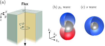
Refer to caption — Figure 1: (a) Schematic of the system. The vortex core is located where $x=y=0$ and the semi-infinite 3D SC that occupies $z\geq 0$ . The gap amplitudes for the (b) $s$ - and (c) $p_{z}$ -wave SC, where color means the internal phase of the pair potential. The inner silver sphere indicates the Fermi sphere.

Odd- $\omega$ pairs in a vortex core are generated by a singularity in real space, whereas odd- $\omega$ pairs at the surface generate ABSs, which are related to anisotropy in the momentum space. The two types of odd- $\omega$ pairs were considered separately¹¹ 1 The vortex shadow effectGraser et al. 2004; Yokoyama et al. 2008b; Silaev et al. 2009 was discussed. However, odd- $\omega$ pairs are not in the same location. . However, these odd- $\omega$ pairs can emerge at the same location and interact with each other. Recently, $k_{z}$ -dependent anisotropic pairings in three-dimensional (3D) SCs have become realistic (e.g., heavy-fermion compoundsRan et al. 2019 and Sr₂RuO₄Pustogow et al. 2019; Suh et al. 2020; Grinenko et al. 2021a; Grinenko et al. 2021b). In these systems, a quantum vortex can penetrate a two-dimensional (2D) surface hosting flat-band ABSs Kobayashi et al. 2015; Tamura et al. 2017; Suzuki et al. 2020; Suzuki et al. 2022. It is unclear how odd- $\omega$ pairs by ABSs affect the odd- $\omega$ pairs carrying the vortex supercurrent, and vice versa. Such novel vortex states help determine the pairing symmetry of an SC and can be easily examined by existing experimental methods such as scanning tunneling microscopyHess et al. 1989 (STM) and superconducting quantum interference devicesKirtley and Wikswo Jr 1999; Wells et al. 2015 (SQUID).

In this study, the interference between odd- $\omega$ pairs with two different origins is investigated: the quantum vortex and surface ABSs. A quantum flux penetrating a semi-infinite 3D unconventional SC is considered, where the magnetic flux is perpendicular to the surface, at $z=0$ . Using the quasiclassical Eilenberger theory, the vortex supercurrents and local density of states (LDOS) in the $s$ - and $p_{z}$ -wave SCs are compared, where surface ABSs are, respectively, absent and present.

The numerical results show that the vortex supercurrent was reversed near the surface where odd- $\omega$ pairs are dominant. The pair amplitude is analyzed and it is shown that there is local symmetry conversion among the Cooper pairs in the region where the vortex and the ABSs coexist. The LDOS, specifically, how the Caroli-de Gennes-Matricon (CdGM) stateCaroli et al. 1964; Hess et al. 1989; Gygi and Schlüter 1991 and surface ABSs develop when they overlap is investigated. It is also shown that the zero-energy peak in the LDOS split because of the interference.

In the analytical calculations, the knowledge gained from the numerical results is extended to more general SCs. By using the Kramer-Pesch approximationKramer and Pesch 1974; Nagai et al. 2006; Nagai and Kato 2019, which is valid at a low temperature and near the vortex core, the direction of the vortex supercurrent near the surface is shown to be determined only by the $k_{z}$ dependence of the pair potential.

The remainder of this paper is organized as follows. The model and method are introduced in Sec. II. The numerical and analytical results are presented in Sec. III and Sec. IV. In Sec. V, the study is summarized.

II System and formulation

We considered the quantum vortex penetrating a 3D SC as shown in Fig. 1(a). The SC occupies $z\geq 0$ and the vortex core is located at $x=y=0$ . We assume the cylindrical symmetry around the core. We employ the cylindrical coordinate: $(x,y,z)=(\rho\cos\Phi,\rho\sin\Phi,z)$ .

The superconductivity in the ballistic limit can be described by quasiclassical Eilenberger theoryEilenberger 1968; Eilenberger and Büttner 1969; Larkin and Ovchinnikov 1969; Schopohl and Maki 1995; Schopohl 1998 . The quasiclassical Green’s function obeys the Eilenberger equation:

		$\displaystyle\hbar\boldsymbol{v}_{F}\cdot\boldsymbol{\nabla}\hat{g}+[\hat{H},\hat{g}]=0,\quad\hat{g}^{2}=\hat{1}$		(1)
		$\displaystyle\hat{g}=\left(\begin{array}[]{cc}g&-s_{\mu}f\\ -\undertilde{f}&-\undertilde{g}\end{array}\right),\quad s_{\mu}=\biggl\{\begin{array}[]{ll}+1&\text{for $s$ wave, }\\ -1&\text{for $p_{z}$ wave, }\end{array}$
		$\displaystyle\hat{H}=\left(\begin{array}[]{cc}\omega_{n}-i(e/c)\boldsymbol{v}_{F}\cdot\boldsymbol{A}&-s_{\mu}\Delta\\ -\undertilde{\Delta}&-\omega_{n}+i(e/c)\boldsymbol{v}_{F}\cdot\boldsymbol{A}\end{array}\right),$

where $\boldsymbol{v}_{F}=v_{F}\hat{\boldsymbol{k}}$ with $\hat{\boldsymbol{k}}=(k_{x},k_{y},k_{z})=(\sin\theta\cos\phi,\sin\theta\sin\phi,\cos\theta)$ , $\omega_{n}=(2n+1)k_{B}T$ , $T$ , $e<0$ , $c$ , and $\boldsymbol{A}$ are the isotropic Fermi velocity, Matsubara frequency, charge of a quasiparticle, speed of light, and vector potential. The normal and anomalous Green’s functions [ $g(\hat{\boldsymbol{k}},\boldsymbol{r},i\omega_{n})$ and $f(\hat{\boldsymbol{k}},\boldsymbol{r},i\omega_{n})$ ] describe the quasiparticle and the Cooper pairs. The under-tilde functions have been introduced as $\undertilde{X}(\hat{\boldsymbol{k}},\boldsymbol{r},i\omega_{n})=X^{*}(-\hat{\boldsymbol{k}},\boldsymbol{r},i\omega_{n})$ with X being an arbitral function. In this paper, we refer to $f$ as the pair amplitude. In Eq. (1), we have reduced the spin degree of freedom by assuming the opposite-spin Cooper pairing for both SCs.

Figure 2: Vector plots of the current densities at

T/T_{c}=0.2

for (a) the

p_{z}

-wave and (b)

s

-wave SCs. The direction and color of the arrows mean the direction and azimuthal component of the current density. The current density is normalised as

\bar{j}_{\Phi}=j_{\Phi}/j^{\mathrm{Max}}_{\Phi}(T/T_{c}=0.2)

with

j^{\mathrm{Max}}_{\Phi}(T/T_{c}=0.2)

being the maximum value of

j_{\Phi}

T/T_{c}=0.2

in each case. The solid black arrows represent the magnetic flux. (c) Top view of the same results at

z=0

and

z\gg\xi

. The parameters are set to

\Omega_{c}=40k_{B}T_{c}

and

\kappa_{\mathrm{GL}}=6\sqrt{6}

We consider the spin-singlet $s$ -wave and spin-triplet $p_{z}$ -wave SCs whose pair potentials can be given by

\displaystyle\Delta(\boldsymbol{r},\hat{\boldsymbol{k}})=\left\{\begin{array}[]{ll}\Delta(\boldsymbol{r})&\text{for $s$ wave,}\\ \Delta(\boldsymbol{r})k_{z}&\text{for $p_{z}$ wave.}\end{array}\right.

The schematic gap functions are shown in Fig. 1. The pair potential $\Delta(\boldsymbol{r})$ is self-consistently determined by the gap equation:

	$\displaystyle\Delta(\hat{\boldsymbol{k}},\boldsymbol{r})$	$\displaystyle=2\lambda N_{0}\pi k_{B}T\sum_{n=0}^{N_{\mathrm{c}}}\int\frac{d\Omega^{\prime}}{4\pi}V(\hat{\boldsymbol{k}},\hat{\boldsymbol{k}}^{\prime})f(\boldsymbol{k}^{\prime},\boldsymbol{r},i\omega_{n}),$		(10)
	$\displaystyle\lambda$	$\displaystyle=N_{0}^{-1}\left(\sum_{n=0}^{N_{\mathrm{c}}}\frac{1}{n+1/2}+\ln\frac{T}{T_{c}}\right)^{-1},$

where $\int\cdots d\Omega/4\pi$ is the average on the Fermi sphere, $N_{0}$ is a density of states (DOS) at Fermi energy in the normal state, and $N_{c}$ is defined as the positive integer satisfying $N_{c}<\Omega_{c}/2\pi k_{B}T$ with $\Omega_{c}$ being the cut-off frequency. The attractive potential $V$ depends on the pairing symmetry: $V=1$ for the $s$ -wave SC and $V=3k_{z}k_{z}^{\prime}$ for the $p_{z}$ wave SC. The pair potential winds its phase around the vortex; $\Delta(\boldsymbol{r})=\Delta(z,\rho)e^{-i\Phi}$ with $(x,y,z)=(\rho\cos\Phi,\rho\sin\Phi,z)$ .

The current density $\boldsymbol{j}(\boldsymbol{r})$ and LDOS $N(\boldsymbol{r},\omega)$ are given by

		$\displaystyle\boldsymbol{j}(\boldsymbol{r})=-4\|e\|N_{0}\pi k_{B}T\sum_{n=0}^{N_{\mathrm{c}}}\int\frac{d\Omega}{4\pi}\boldsymbol{v}_{F}\cdot\mathrm{Im}g(\hat{\boldsymbol{k}},\boldsymbol{r},\omega_{n}),$		(11)
		$\displaystyle\frac{N(\boldsymbol{r},\omega)}{N_{0}}=\lim_{\delta\rightarrow+0}\int\frac{d\Omega}{4\pi}\mathrm{Re}\left[g(\hat{\boldsymbol{k}},\boldsymbol{r},\omega+i\delta)\right].$		(12)

where $\delta$ is the smearing factor. The vector potential is also self-consistently determined using the following equations:

\displaystyle\boldsymbol{\nabla}\times\boldsymbol{A}=\boldsymbol{B},\hskip 17.07164pt\boldsymbol{\nabla}\times\boldsymbol{B}=\frac{4\pi}{c}\boldsymbol{j}.

(13)

In the quasiclassical theory, the Ginzburg-Landau (GL) parameter $\kappa=\lambda_{L}/\xi$ is a parameter that characterizes the length scale of the magnetic field, where $\lambda_{L}=\sqrt{3c^{2}/8\pi e^{2}v_{F}^{2}N_{0}}$ and $\xi=\hbar v_{F}/2\pi k_{B}T_{c}$ are the London penetration depth and coherence length (see the Appendix A for the detail). In the numerical calculations, we set $\kappa=6\sqrt{6}$ and $\Omega_{c}=40k_{B}T_{c}$ .

III Numerical Results

III.1 Paramagnetic quantum vortex

Figure 3: Spatial profiles of (a) the circulation current and (b) the magnetic field in the

p_{z}

-wave SC. The magnetic field is normalized as

\bar{B}_{z}=B_{z}/B_{z}(\rho=0,z=10\xi,T/T_{c}=0.2)

. The depth is set to

z/\xi=0,1,2,4

, and

10

. Near the surface, the current changes the direction and the magnetic field is significantly suppressed. The depth dependence of

\bar{W}_{B}

is shown in the inset.

The vector plot of the current density around the vortex core in the $p_{z}$ -wave SC is shown in Fig. 2(a), where the result for the $s$ -wave SC is shown in Fig. 2(b) as a reference. The color of the vectors corresponds to $j_{\Phi}$ : the red and blue mean the diamagnetic and paramagnetic current respectively. At the surface of the $p_{z}$ -wave SC, the current density changes its direction near the surface as shown in Fig. 2(a), whereas $\boldsymbol{j}$ in the $s$ -wave case hardly depends on $z$ as shown in Fig. 2(b). The vortex supercurrent inversion can be seen more clearly in the top views in Fig. 2(c). The $\rho$ dependence of $j_{\Phi}$ for the $p_{z}$ -wave SC is shown in Fig. 3(a), where we fixed the depth at $z/\xi=0,1,2,4,10$ . We see that the profile of $j_{\Phi}$ at $z=10\xi$ is qualitatively the save as the well-known $s$ -wave result Gygi and Schlüter 1991. However, with approaching to the surface, $j_{\Phi}$ changes the sign at $z\sim 2\xi$ , meaning that the paramagnetic current flows only near the surface. The self-consistent pair potentials are shown in the Appendix B.

The $z$ component of the local magnetic field $B_{z}$ for the $p_{z}$ -wave SC is shown in Fig. 3(b). Deep inside the SC, $B_{z}$ has the typical profile: the magnetic field has a peak at the vortex core and decays in the order of $\lambda_{L}$ . However, with approaching to the surface, $B_{z}$ is strongly suppressed and spreads broader. Although the paramagnetic current flows near the surface, it does not change $\mathrm{sgn}[B_{z}]$ but modifies significantly the spatial profile of $B_{z}$ at the surface. We show that the width of the peak in $B_{z}$ strongly depends on $z$ as in the inset of Fig. 3, where the peak width $W_{B}$ is defined by using the half-value radius; $B_{z}|_{\rho=W_{B}}=(1/2)B_{z}|_{\rho=0}$ . In the $s$ -wave case, the peak width does not strongly depends on $z$ . On the contrary, it depends significantly on $z$ in the $p_{z}$ -wave case. At the surface, $W_{B}$ is about four times larger than its value at $z=10\xi$ .

The temperature dependence of $j_{\Phi}$ is shown in Fig. 4(a), where $j_{\Phi}$ is obtained at the surface of the $p_{z}$ -wave SC. The amplitude of the paramagnetic current increases with decreasing temperature. In particular, the paramagnetic current increases rapidly at low temperature. This low-temperature anomaly is characteristic to the paramagnetic response related to the odd- $\omega$ pairs induced by the ABSs Asano et al. 2011; Higashitani et al. 2013; Higashitani 2014a; Suzuki and Asano 2014; Suzuki and Asano 2015.

Figure 4: (a) Paramagnetic vortex-current at the surface of the

p_{z}

-wave SC. The current density is normalized as

\tilde{j}=j_{\Phi}/|j_{\Phi}^{\mathrm{Min}}(T/T_{c}=0.2)|

with

j_{\Phi}^{\mathrm{Min}}(T/T_{c}=0.2)

being the minimum value of

j_{\Phi}

T/T_{c}=0.2

. The temperature is set to

T/T_{c}=0.2,0.4,0.6

and

0.7

. The open squares indicate the maximum value of

|j_{\Phi}(\rho,z=0)|

at each temperature. (b) Magnetic field at the surface of the

p_{z}

- and

s

-wave SCs. The temperature in the

p_{z}

-wave SC is set to

T/T_{c}=0.2,0.4,0.6

and

0.8

, and the temperature in the

s

-wave SC is

T/T_{c}=0.2

. Insets in (a) and (b) show the temperature dependences of

W_{J}

and

W_{B}

, where

W_{J}

is defined as

|j_{\Phi}(\rho=W_{J},z=0,T)|=\max_{\rho}|j_{\Phi}(\rho,z=0,T)|

. We normalize

W_{J(B)}

\bar{W}_{J(B)}(T/T_{c}=0.8)=W_{J(B)}/W_{J(B)}(T/T_{c}=0.8)

in each SC.

Figure 5: Pair amplitudes at (a,b)

z=10\xi

and (c,d)

z=0

. The left (right) figures show the even frequency (odd parity) components. The parameters are set to

T=0.2T_{c}

\omega_{n}=\omega_{0}

, and

\Phi=0

. The definition and notation of

C_{lm}(\boldsymbol{r})

are shown in Eq. (14) and the Appendix C. The even- and odd-frequency components are subdominant at

z=0

and

z=10\xi

respectively. The other components are negligibly small.

III.2 Symmetry conversion

We explore the origin of the paramagnetic circulating current in this subsection. The magnetic response is related to the frequency symmetry of Cooper pairs Asano et al. 2011; Yokoyama et al. 2011; Higashitani et al. 2013; Higashitani 2014a; Suzuki and Asano 2014; Suzuki and Asano 2015; Asano and Sasaki 2015. Namely, the direction of the vortex current is determined by the spatial distribution of the even- and odd- $\omega$ Cooper pairs. To analyze the symmetry of the Cooper pairs, we expand the pair amplitudes at $\omega_{0}$ in terms of the real spherical harmonics (See Appendix C for the details):

\displaystyle f(\boldsymbol{r},\boldsymbol{k},\omega_{0})=\sum_{lm}f_{lm}(\boldsymbol{r},\boldsymbol{k}),

\displaystyle f_{lm}=C_{lm}(\boldsymbol{r})Y_{lm}(\boldsymbol{k}).

(14)

We refer to, for example, $f_{l=2,m=2}$ ( $d_{x^{2}-y^{2}}$ -wave component) as $f_{x^{2}-y^{2}}$ for simplicity. We hereafter fix $\Phi=0$ because of the rotational symmetry around the vortex.

Deep inside the $p_{z}$ -wave SC, the symmetry conversion is caused only by the vortex singularity at $\rho=0$ . In the homogeneous limit, the pair amplitude has only the $p_{z}$ -wave component: $f=\Delta_{\infty}k_{z}/\sqrt{\omega_{n}^{2}+\Delta_{\infty}k_{z}^{2}}\sim f_{z}+f_{z^{3}}$ with $\Delta_{\infty}$ being the pair potential in the homogeneous limit, where the denominator induces non- $p_{z}$ -wave component. At the vortex core, the pair amplitude obtains an additional phase from the phase winding of the vortex: $f\sim k_{z}(k_{x}+ik_{y})\sim f_{zx}+if_{yz}$ Yokoyama et al. 2008a; Tanuma et al. 2009. In a spin-triplet SC, these even-parity components should be an odd function of $\omega_{n}$ to satisfy the Pauli exclusion principal (i.e., Berezinskii ruleBerezinskii). Figure 5(a) and 5(b) show the symmetry conversion between the even- and odd- $\omega$ components at $z=10\xi$ . The even- $\omega$ $p_{z}$ -wave component is dominant at $\rho\gg\xi$ , whereas only the odd- $\omega$ $d_{zx}+id_{yz}$ -wave component has an amplitude at $\rho=0$ .

At the surface, the symmetry conversion is caused by the two factors: the surface ABSs and vortex. The pairing symmetry is shown in Figs. 5(c) and 5(d). At $\rho\gg\xi$ , the pair amplitude can be written as a superposition of the $s$ -wave and $d$ -wave pairings Tanaka et al. 2007; Suzuki and Asano 2014; Suzuki and Asano 2015: $f\sim f_{0}+f_{z^{2}}$ . Namely, only the odd- $\omega$ pairs are present at the surface far from a vortex. At the intersection of the vortex core and surface (i.e., $\rho=z=0$ ), these odd- $\omega$ pairs have an additional phase from the vortex. As a result, the $p_{x}+ip_{y}$ -wave and $f_{xz^{2}}+if_{yz^{2}}$ are dominant as shown in Fig. 5(c). Note that these even- $\omega$ pairs are generated from the odd- $\omega$ pairs, and have different pairing symmetry from the pair potential.

The relation between the frequency-symmetry conversion and supercurrent inversion can be confirmed by analyzing the current density $\boldsymbol{j}$ in Eq. (11). Close to the vortex core (i.e., $\rho\ll\xi$ ), $\boldsymbol{j}$ can be expressed in terms of the pair amplitudes Higashitani 2014b; Suzuki and Asano 2014; Suzuki and Asano 2016. Specifically, it can be expressed by the even- $\omega$ (odd- $\omega$ ) component $f_{e(o)}$ :

		$\displaystyle j_{\Phi}(\boldsymbol{r})=-j_{0}\frac{T}{T_{c}}\sum_{n=0}^{N_{\mathrm{c}}}\int\frac{d\Omega}{4\pi}\sin\theta\sin\phi\mathrm{Im}g(\hat{\boldsymbol{k}},\boldsymbol{r},\omega_{n}),$		(15)
		$\displaystyle g=\sqrt{1-\|f_{e}\|^{2}+\|f_{o}\|^{2}-2i\mathrm{Im}f_{o}f_{e}^{*}},$		(16)
		$\displaystyle f_{e(o)}=\frac{1}{2}[f(\boldsymbol{r},\boldsymbol{k},\omega_{n})+(-)f(\boldsymbol{r},\boldsymbol{k},-\omega_{n})]$		(17)

where we have used the normalization condition (i.e., $g^{2}=1-s_{\mu}f\undertilde{f}$ ) and $j_{0}={4\pi N_{0}|e|v_{F}T_{c}}$ . In the Appendix D, applying the conversion $f_{e}\leftrightarrow f_{o}$ to Eqs. (15) and (16), we have shown that the frequency-symmetry conversion by the surface ABSs results in the vortex-current inversion.

III.3 Local density of states

Before discussing the obtained results, we quickly overview the in-gap states related to this system: surface ABS and CdGM mode. The $p_{z}$ -wave SC hosts the surface ABSsHara and Nagai 1986 at its surface perpendicular to the $z$ -direction because of the quasiparticle interference ²² 2 At a surface of an SC, the incoming and outgoing quasiparticles interfere. These two quasiparticles feel, in general, different pair potentials depending on the momentum: $\Delta(k_{z},\boldsymbol{k}_{\parallel})$ and $\Delta(-k_{z},\boldsymbol{k}_{\parallel})$ where the surface is perpendicular to the $z$ axis. In the $p_{z}$ -wave SC, the phase difference between these two pair potentials is $\pi$ : $\Delta(k_{z},\boldsymbol{k}_{\parallel})=-\Delta(-k_{z},\boldsymbol{k}_{\parallel})$ . The $\pi$ -phase shift results in forming the surface bound state at the zero energy.. In the $p_{z}$ -wave case, the ABSs form the flat-band zero-energy surface statesHu 1994; Kashiwaya and Tanaka 2000; Sato et al. 2011. The CdGM modes are quasiparticle states bounded at a vortex coreCaroli et al. 1964. Because of the confinement by the local suppression in the pair potential, the in-gap quasiparticle states appears at the vortex core ³³ 3 The energy levels for the CdGM modes are given by $E=\pm(n-1/2)\Delta_{\infty}^{2}/E_{F}$ . In the quasiclassical regime, the lowest CdGM mode seem to sit at $E=0$ because $\Delta/E_{F}\ll 1$ is assumed in the quasiclassical theory. . In the Appendix B, we show the quasiparticle spectra of the $s$ -wave SC with a vortex as a reference, where we explain the spatial distribution of the CdGM modes.

The LDOS at the surface of the $p_{z}$ -wave SC are shown in Fig. 6, which can be measured by, for example, a scanning tunnel spectroscopy measurement. The flat-band zero-energy ABSs appear at far from the vortex core (i.e., $\rho\gg\xi$ ). Approaching to the vortex, the bound-states energy is lifted from $E=0$ and the zero-energy peak is split into two peaks with $E\approx 0.5\Delta_{\infty}$ at $\rho=0$ . The evolution of the CdGM modes at the lowest energy are shown in Fig. 6, where we fix $\rho=0$ . Deep inside the SC ( $z\gg\xi$ ), the CdGM mode stay at $E\approx 0$ . However, with approaching to the surface, the zero-energy peak splits into two peaks.

We conclude the zero-energy peak splitting is a result of the interference between the surface ABSs from the $p_{z}$ -wave nature and the CdGM modes from the quantum vortex: the quantum states staying at $E=0$ repel each other in energy space due to the superposition in real space.

The splitting of the LDOS at $E=0$ can also be interpreted in another way. The ABS appears at the zero-energy when $\Delta(\boldsymbol{k}_{\mathrm{in}})=-\Delta(\boldsymbol{k}_{\mathrm{out}})$ during the reflection at a surface, where $\boldsymbol{k}_{\mathrm{in}}$ ( $\boldsymbol{k}_{\mathrm{out}}$ ) is the incoming (outgoing) momentum. A similar sign change occurs when the quasiparticle passes through the vortex core. However, on the quasiclassical paths passing through the origin (intersection of the surface and the vortex core), this sign change never occurs. The sign change from the reflection and that from the vortex core compensate each other. Therefore, the zero-energy state does not appear at the origin.

IV Kramer-Pesch theory

We apply the Kramer-Pesch approximationKramer and Pesch 1974; Nagai et al. 2006; Nagai and Kato 2019 to more general superconducting states and generalize our results obtained numerically; the vortex-current reversal and disappearance of the zero-energy peak at $z=\rho=0$ in the LDOS. The Kramer-Pesch approximation, which is valid when $k_{B}T\ll|\Delta_{\infty}|$ and $\rho\ll\xi$ , allow us to obtain the analytic solution of the quasiclassical Green’s function. We assume that the gap function is written as

\displaystyle\Delta(\boldsymbol{r},\hat{\boldsymbol{k}})=h(\rho,z)e^{-i\Phi}\Psi(\hat{\boldsymbol{k}}),

(18)

where $h(\rho,z)$ is a real function describing the spatial profile of $\Delta$ and $\Psi(\hat{\boldsymbol{k}})$ is the momentum dependence of $\Delta$ which satisfies $\Psi(\boldsymbol{k}_{\parallel},k_{z})=s_{\theta}\Psi(\boldsymbol{k}_{\parallel},-k_{z})$ with $\boldsymbol{k}_{\parallel}=(k_{x},k_{y},0)$ and $s_{\theta}=\pm 1$ . Surface ABSs are formed when $s_{\theta}=-1$ . In the Kramer-Pesch approximation, the azimuthal components of current density $j_{\Phi}$ for each $s_{\theta}$ are written as

$\displaystyle j_{\Phi}(\boldsymbol{r})\|_{s_{\theta}=1}$	$\displaystyle\simeq 4\pi N_{0}\|e\|v_{F}\int\frac{d\Omega}{4\pi}\sin^{2}(\phi-\Phi)\frac{C^{-1}}{4k_{B}T}\rho\tilde{D},$	(19)
$\displaystyle j_{\Phi}(\boldsymbol{r})\|_{s_{\theta}=-1}$	$\displaystyle\leq 4\pi N_{0}\|e\|v_{F}\int\frac{d\Omega}{4\pi}\sin^{2}(\phi-\Phi)\left[-\frac{C^{-1}}{8k_{B}T}+\frac{2}{C^{-1}}\right]\rho\tilde{D},$	(20)
$\displaystyle\tilde{D}(\rho,\Phi,\boldsymbol{k})$	$\displaystyle=\frac{2}{v_{F}C(\rho,\Phi,\boldsymbol{k})}\int^{\infty}_{-\infty}d\sigma^{\prime}\frac{1}{\sigma^{\prime}}h\left(\|\sigma\|\sin\theta,\left\|\sigma\cos\theta-\rho\frac{\cos(\phi-\Phi)}{\tan\theta}\right\|\right)\exp\left[-2\|\Psi(\boldsymbol{k})\|\bar{F}(\rho,\Phi,\sigma^{\prime},\boldsymbol{k})\right],$	(21)
$\displaystyle C(\rho,\Phi,\boldsymbol{k})$	$\displaystyle=\frac{2}{v_{F}}\int^{\infty}_{-\infty}d\sigma^{\prime}\exp\left[-2\|\Psi(\boldsymbol{k})\|\bar{F}(\rho,\Phi,\sigma^{\prime},\boldsymbol{k})\right],$	(22)
$\displaystyle\bar{F}(\rho,\Phi,\sigma,\hat{\boldsymbol{k}})$	$\displaystyle=\int_{\rho\cos(\phi-\Phi)(\sin\theta)^{-1}}^{\sigma}\mathrm{sign}(\sigma^{\prime})h(\|\sigma^{\prime}\|\sin\theta,\|\sigma^{\prime}\cos\theta+z_{0}\|)d\sigma^{\prime},$	(23)

where $\tilde{D}\geq 0$ and $C\geq 0$ . The detailed derivation of Eq. (20) is explained in the Appendix E. The conventional vortex current has a positive value as in Eq. (19). On the other hand, Eq. (20) shows that the current density can be negative at low temperature because of the first term. Thus, the vortex current on the surface with the ABS is reversed.

In the Kramer-Pesch approximation, the surface DOS for $s_{\theta}=-1$ is written as

	$\displaystyle\frac{N(E,\rho,z=0)}{N_{0}}$	$\displaystyle=\int\frac{d\Omega}{4\pi}\frac{(\rho D+E)^{2}}{(\rho D+E)^{2}+C^{-2}}\leq 1,$		(24)
	$\displaystyle D$	$\displaystyle=\frac{\sin(\phi-\Phi)}{\sin\theta}\tilde{D}.$		(25)

Equation (24) shows that the surface DOS is less than $N_{0}$ and becomes zero at $\rho=E=0$ (see the Appendix E for the details.). Therefore, the zero-energy peak in the LDOS at $\rho=z=0$ disappears when $s_{\theta}=-1$ .

Applying the Kramer-Pesch approximation, we demonstrate the current inversion and the disappearance of the zero-energy peak in the LDOS under the condition $\Delta(k_{x},k_{y},k_{z})=-\Delta(k_{x},k_{y},-k_{z})$ . This indicates that our numerical results are not unique only to the $p_{z}$ -wave SC. The vortex supercurrent inversion can occur in superconductors with flat-band surface ABSs.

V Conclusion

We have demonstrated that the local frequency-symmetry conversion of Cooper pairs inverts the direction of the vortex supercurrent. Using the quasiclassical Eilenberger theory, a quantum vortex penetrating a surface hosting the ABSs both numerically and analytically has been investigated. In the self-consistent simulations, comparing the vortex supercurrents in the $p_{z}$ -wave and $s$ -wave SCs, we have found that the supercurrent flows in the opposite direction near the surface of the $p_{z}$ -wave SC. By analyzing the anomalous Green’s function, the frequency-symmetry conversion among Cooper pairs by ABSs has been shown to trigger the supercurrent inversion. In the analytic calculation with the Kramer-Pesch approximation, the condition of the vortex current inversion has been generalized.

From the quasiparticle spectra obtained from the Green’s function, we have found that the zero-energy states from the ABSs and CdGM mode are coupled with each other and shift to non-zero energies when the current inversion occurred. Within the Kramer-Pesch approximation, it has been analytically shown that the LDOS is zero at the intersection of the vortex core and surface because of the interference between the ABSs and CdGM mode.

Acknowledgements.

The authors are thank A. A. Golubov for the fruitful discussions. S. Y. would like to take this opportunity to thank the “Nagoya University Interdisciplinary Frontier Fellowship” supported by JST and Nagoya University. S.-I. S. is supported by JSPS Postdoctoral Fellowship for Overseas Researchers and a Grant-in-Aid for JSPS Fellows (JSPS KAKENHI Grant No. JP19J02005). This work was supported by Scientific Research (A) (KAKENHI Grant No. JP20H00131), and Scientific Research (B) (KAKENHI Grant No. JP20H01857).

Appendix A Maxwell equation, Riccati parametrization, and boundary conditions

In this section, we introduce the formulations of the vector potential, Riccati parametrization, and boundary conditions. Under the rotational symmetry around the $z$ axis, the magnetic field $\boldsymbol{B}$ and vector potential $\boldsymbol{A}$ are obtained from $\boldsymbol{j}$ as

$\displaystyle\boldsymbol{B}(\boldsymbol{r})$	$\displaystyle=\frac{1}{c}\int\boldsymbol{j}(\boldsymbol{r}^{\prime})\times\frac{\boldsymbol{r}-\boldsymbol{r}^{\prime}}{\left\|\boldsymbol{r}-\boldsymbol{r}^{\prime}\right\|^{3}}dV^{\prime},$	(26)
$\displaystyle\boldsymbol{A}(\boldsymbol{r})$	$\displaystyle=\boldsymbol{e}_{\Theta}\int_{z}^{\infty}B_{\rho}(\rho,z^{\prime})dz^{\prime}$
	$\displaystyle\hskip 17.07164pt+\boldsymbol{e}_{\Theta}\frac{1}{\rho}\int_{0}^{\rho}\rho^{\prime}B_{z}(\rho^{\prime},z=\infty)d\rho^{\prime}.$	(27)

We introduce a dimensionless Maxwell equation (13) for numerical calculations:

\displaystyle\boldsymbol{\nabla}^{\prime}\times\left(\boldsymbol{\nabla}^{\prime}\times\boldsymbol{A}^{\prime}\right)=\frac{6}{\kappa^{2}}\boldsymbol{j}^{\prime},

(28)

where $\boldsymbol{\nabla}^{\prime}=\xi\boldsymbol{\nabla}$ , $\boldsymbol{A}$ and $\boldsymbol{j}$ are normalized as $\boldsymbol{A}^{\prime}=(2\pi\xi/\Phi_{0})\boldsymbol{A}$ and $\boldsymbol{j}^{\prime}=\boldsymbol{j}/j_{0}$ with $\Phi_{0}=\pi\hbar c/|e|$ and $j_{0}=4\pi N_{0}|e|v_{F}T_{c}$ .

In order to solve the Eilenberger equation (1) numerically, we introduce the coherence functionSchopohl and Maki 1995; Schopohl 1998 $\gamma$ as

\displaystyle g

\displaystyle=\frac{1-s_{\mu}\gamma\undertilde{\gamma}}{1+s_{\mu}\gamma\undertilde{\gamma}},\quad f=\frac{2\gamma}{1+s_{\mu}\gamma\undertilde{\gamma}}.

(29)

Substituting Eq. (29) into Eq. (1), we obtain the Riccati-type differential equations:

	$\displaystyle\hbar\boldsymbol{v}_{F}\cdot\boldsymbol{\nabla}\gamma-2\left(\omega_{n}-\frac{ie}{c}\boldsymbol{v}_{F}\cdot\boldsymbol{A}\right)\gamma-\Delta+\Delta^{*}\gamma^{2}=0,$		(30)
	$\displaystyle\hbar\boldsymbol{v}_{F}\cdot\boldsymbol{\nabla}\undertilde{\gamma}+2\left(\omega_{n}-\frac{ie}{c}\boldsymbol{v}_{F}\cdot\boldsymbol{A}\right)\undertilde{\gamma}+s_{\mu}\Delta^{*}-s_{\mu}\Delta\undertilde{\gamma}^{2}=0.$		(31)

The solutions of Eq. (1) are given by solving Eq. (30) and (31) along the quasiclassical paths and substituting the obtained $\gamma$ and $\undertilde{\gamma}$ into Eq. (29). We solve Eqs. (10), (27), (30) and (31) numerically in a self-consistent manner. The coherence functions $\gamma$ and $\undertilde{\gamma}$ in the homogeneous limit (i.e., $\nabla\cdot\gamma=0$ ) are given by

	$\displaystyle\gamma$	$\displaystyle=\frac{\Delta_{\infty}}{\omega_{n}+\mathrm{sign}(\omega_{n})\sqrt{\omega_{n}^{2}+\|\Delta_{\infty}\|^{2}}},$		(32)
	$\displaystyle\undertilde{\gamma}$	$\displaystyle=\frac{s_{\mu}\Delta_{\infty}^{*}}{\omega_{n}+\mathrm{sign}(\omega_{n})\sqrt{\omega_{n}^{2}+\|\Delta_{\infty}\|^{2}}},$		(33)

where $\Delta_{\infty}$ is the bulk value of $\Delta$ .

We impose the boundary conditions on the coherence functions. (I) The coherence functions are equal to the values in Eqs. (32) and (33) deep inside the SC (i.e., $\rho\gg\xi,~z\gg\xi$ ). (II) At the surface (i.e., $z=0$ ), we impose

\displaystyle\gamma(\hat{\boldsymbol{k}}_{\parallel},\hat{\boldsymbol{k}}_{z},\boldsymbol{r}_{\parallel},z=0,\omega_{n})=\gamma(\hat{\boldsymbol{k}}_{\parallel},-\hat{\boldsymbol{k}}_{z},\boldsymbol{r}_{\parallel},z=0,\omega_{n}),

(34)

which means the specular reflection where $\boldsymbol{r}_{\parallel}=(x,y)$ . As a result of Eq. (34), the pair amplitude $f$ is forced to be an even function with respects to the $k_{z}$ inversion at the surface.

Appendix B Additional numerical results

In this section, we show the spatial dependence of the pair potential and local density of state (LDOS) for the $s$ -wave SC. We show the spatial dependences of the pair potential in Fig. 7. As show in Fig. 7(a), the pair potential in the $s$ -wave SC is suppressed near the vortex core but not at the surface. On the other hand, the pair function in the $p_{z}$ -wave SC disappears at the vortex core and the surface as shown in Fig. 7(b).

In Fig. 8, we show the LDOS in the $s$ -wave SC. Figures 8(a) and (b) show the LDOS at the surface and vortex core. In Fig. 8, there exist sub-gap bound states near the core known as the Caroli-de-Gennes-Matricon (CdGM) modes. The approximate energy dispersion of the CdGM modes have been derived as $E_{n}\simeq(n-1/2)\Delta_{\infty}^{2}/E_{F}$ in Ref. Caroli et al. 1964, where the half integer $(n-1/2)$ is the quantum number of the angular momentum. The eigenfunction of the CdGM mode labeled by $n$ has a maximum amplitude at a radius distance of the order $\rho\simeq(n-1/2)/k_{F}$ Gygi and Schlüter 1991. Thus, the evolution of sub-gap states in Fig. 8(a) corresponds to the dispersion relation of the CdGM modes.

Appendix C Renormalized spherical harmonics

We use the real spherical harmonics $Y_{lm}$ to analyze the pair amplitudes. We abbreviate the expansion coefficients $f_{lm}$ in the main texts for simplicity. We summarize $Y_{lm}$ and the notation of $f_{lm}$ in Table 1. The spherical harmonics $Y_{lm}$ is normalized to satisfy the orthonormal relation

\displaystyle\int Y_{lm}Y_{l^{\prime}m^{\prime}}d\Omega=\delta_{ll^{\prime}}\delta_{mm^{\prime}},

(35)

where $d\Omega=\sin\theta d\phi d\theta$ .

Table 1: Notation of the expansion coefficients

f_{lm}

Appendix D Vortex supercurrent and frequency symmetry of Cooper pairs

The direction of the vortex supercurrent is related to the frequency symmetry of Cooper pairs. The azimuthal component of the current density (11) is

\displaystyle j_{\Phi}(\boldsymbol{r})=-j_{0}\frac{T}{T_{c}}\sum_{n=0}^{N_{\mathrm{c}}}\int\frac{d\Omega}{4\pi}\sin\theta\sin\phi\mathrm{Im}g(\hat{\boldsymbol{k}},\boldsymbol{r},\omega_{n}),

(36)

where $j_{0}={4\pi N_{0}|e|v_{F}T_{c}}$ . Namely, the direction of the current is determined by the sign of $\mathrm{Im}[g]$ . Using the normalization condition for the quasiclassical Green’s function (i.e., $g^{2}=1-s_{\mu}f\undertilde{f}$ ), we have

		$\displaystyle g=\sqrt{1-\|f_{e}\|^{2}+\|f_{o}\|^{2}-2i\mathrm{Im}f_{o}f_{e}^{*}},$		(37)
		$\displaystyle f_{e(o)}=\frac{1}{2}[f(\boldsymbol{r},\boldsymbol{k},\omega)+(-)f(\boldsymbol{r},\boldsymbol{k},-\omega)],$		(38)

where $f_{e}$ and $f_{o}$ represent respectively the even- and odd-frequency component, and we have used the symmetry relation between $f$ and $\undertilde{f}$ [i.e., $\undertilde{f}(\boldsymbol{r},\boldsymbol{k},\omega)=f^{*}(\boldsymbol{r},-\boldsymbol{k},\omega)$ ].

Figure 9: Schematic picture of the spatial distribution of the pair amplitudes around the vortex in the

p_{z}

-wave SC. The even and odd-

\omega

pairs are dominant near the vortex core at the surface and deep inside the SC.

We analyze the direction of the vortex supercurrent in the vicinity of the vortex core. From Fig. 9, deep inside the SC, the pair amplitudes around the vortex core can be approximated as

\displaystyle f_{e}\approx\rho F,\quad f_{o}\approx-RFe^{-i\phi},

(39)

where $F=F(\hat{\boldsymbol{k}})$ and we have introduced the constant $R$ ( $0<R<1$ ) that expresses the relative amplitude of $f_{o}$ to $f_{e}$ . The subdominant component has an additional phase factor ( $-e^{-i\phi}$ ) from the phase winding of the vortex. Substituting Eq. (39) into Eq. (37), we have

	$\displaystyle g$	$\displaystyle=\sqrt{1-\rho^{2}\|F\|^{2}+R^{2}\|F\|^{2}+2i\rho R\|F\|^{2}\mathrm{Im}e^{-i\phi}}$		(40)
		$\displaystyle=\sqrt{1+R^{2}\|F\|^{2}}-i\rho\frac{R\|F\|^{2}\sin\phi}{\sqrt{1+R^{2}\|F\|^{2}}}+O(\rho^{2})$		(41)

with $\rho\ll\xi$ . The equation above results in

\displaystyle-j_{0}\sin\phi\mathrm{Im}g=\rho\frac{j_{0}R|F|^{2}\sin^{2}\phi}{\sqrt{1+R^{2}|F|^{2}}}+O(\rho^{2}),

(42)

meaning that the electric current flows in the opposite direction of the phase winding $e^{-i\Phi}$ around the vortex core (i.e., $j_{\Phi}>0$ ).

At the surface of a $p_{z}$ -wave SC, the symmetry conversion occurs because of the ABSs. The pair amplitudes can be expressed as

\displaystyle f_{e}=-RFe^{-i\phi},\quad f_{o}=\rho F,

(43)

where we can show $R^{2}|F|^{2}=1$ by solving the Riccati-type differential equations (47) at $T=0$ and $\rho=0$ . We assume $f_{e}$ near the core has the maximum value at $\omega_{n}=0$ . From this assumption, we obtain $R^{2}|F|^{2}<1$ at finite matsubara frequencies. Substituting Eq. (43) into Eq. (37), we have

	$\displaystyle g$	$\displaystyle=\sqrt{1-R^{2}\|F\|^{2}+\rho^{2}\|F\|^{2}+2i\rho R\|F\|^{2}\mathrm{Im}e^{i\phi}}$		(44)
		$\displaystyle=\sqrt{1-R^{2}\|F\|^{2}}+i\rho\frac{R\|F\|^{2}\sin\phi}{\sqrt{1-R^{2}\|F\|^{2}}}+O(\rho^{2}).$		(45)

Therefore, the direction of the current density is given by

\displaystyle-j_{0}\sin\phi\mathrm{Im}[g]=-\rho\frac{j_{0}R|F|^{2}\sin^{2}\phi}{\sqrt{1-R^{2}|F|^{2}}}+O(\rho^{2})

(46)

Comparing Eqs. (42) and (46), we see that the frequency-symmetry conversion results in the vortex-current inversion.

Appendix E Analytical Calculations by Kramer-Pesch approximation

Figure 10: Coordinate transformation from

(x,y,z)

(a,b,z)

In this section, we analytically calculate the quasi-classical Green’s functions by the Kramer-Pesch approximation Kramer and Pesch 1974; Nagai et al. 2006; Nagai and Kato 2019 and reproduce two numerical results, the reversal of the vortex current and suppression of the LDOS at the intersection point of the surface and vortex core, for more general SCs. In the Kramer-Pesch approximation, we obtain the solutions of the Riccati-type differential equations up to the first order of the displacement $b$ from the vortex core and Matsubara frequency $\omega_{n}$ . Thus, the Kramer-Pesch approximation is appropriate near the vortex core $\rho\ll\xi$ and in low temperature $k_{B}T\ll|\Delta|$ . In this section, We follow the method in Ref. Nagai et al. 2006.

We start with the Riccati-type differential equations with $\boldsymbol{A}=0$ :

	$\displaystyle\boldsymbol{v}_{F}\cdot\nabla\gamma+2\omega_{n}\gamma-\Delta+\Delta^{*}\gamma^{2}=0,$		(47)
	$\displaystyle\boldsymbol{v}_{F}\cdot\nabla\undertilde{\gamma}-2\omega_{n}\undertilde{\gamma}+s_{\mu}\Delta^{*}-s_{\mu}\Delta\undertilde{\gamma}^{2}=0,$		(48)

where we use the units $\hbar=k_{B}=1$ . We introduce the coordinate transformation as in Fig.10:

	$\displaystyle a$	$\displaystyle=x\cos\phi+y\sin\phi,$		(49)
	$\displaystyle b$	$\displaystyle=-x\sin\phi+y\cos\phi,$		(50)

where the angle $\phi$ characterizes the direction of the momentum: $\hat{\boldsymbol{k}}=(\sin\theta\cos\phi,\sin\theta\sin\phi,\cos\theta)$ . The $b$ -axis is perpendicular to the projected momentum $\boldsymbol{k}_{\parallel}=(\sin\theta\cos\phi,\sin\theta\sin\phi,0)$ . We solve the Riccati-type differential equations by integrating $\gamma$ or $\undertilde{\gamma}$ in the direction $\hat{\boldsymbol{k}}$ . The impact parameter $b$ is constant on the integrating path and corresponds to the distance between the integrating path and vortex core. In this coordinate $\boldsymbol{r}=(a,b,z)$ , the Riccati-type differential equations are rewritten as

		$\displaystyle v_{F}\left\{\sin\theta\frac{\partial}{\partial a}+\cos\theta\frac{\partial}{\partial z}\right\}\gamma+2\omega_{n}\gamma-\Delta+\Delta^{*}\gamma^{2}=0,$		(51)
		$\displaystyle v_{F}\left\{\sin\theta\frac{\partial}{\partial a}+\cos\theta\frac{\partial}{\partial z}\right\}\undertilde{\gamma}-2\omega_{n}\undertilde{\gamma}+s_{\mu}\Delta^{*}-s_{\mu}\Delta\undertilde{\gamma}^{2}=0.$		(52)

In the analytic calculation, the pair potential is written in more general form:

\displaystyle\Delta(\hat{\boldsymbol{k}})

\displaystyle=h(\rho,z)e^{-i\Phi}\Psi(\hat{\boldsymbol{k}}).

(53)

where the real function $h$ and the complex function $\Psi$ describe the spatial and momentum dependence of $\Delta$ . In addition, we assume that $\Psi$ satisfies $s_{\theta}=\Psi(\theta,\phi)/\Psi(\pi-\theta,\phi)=\pm 1$ . In the case of $s_{\theta}=1$ and $-1$ , the ABSs is absence and present on the surface perpendicular to the $z$ axis. We expand the pair potential as

		$\displaystyle\Delta(\hat{\boldsymbol{k}},\boldsymbol{r})=\Delta_{0}+\Delta_{1},$		(54)
		$\displaystyle\Delta_{0}=h(\|a\|,z)e^{-i\phi}\mathrm{sign}(a)\Psi(\hat{\boldsymbol{k}}),$		(55)
		$\displaystyle\Delta_{1}=-h(\|a\|,z)e^{-i\phi}\mathrm{sign}(a)i\frac{b}{a}\Psi(\hat{\boldsymbol{k}}),$		(56)

with respect to $b$ . The solutions (32) and (33) in the homogeneous limit are also expanded in terms of $b$ and $\omega_{n}$ as

	$\displaystyle\gamma(\boldsymbol{r},\hat{\boldsymbol{k}},\omega_{n})$	$\displaystyle=\mathrm{sign}(a\omega_{n})\left\{\frac{\Psi(\hat{\boldsymbol{k}})e^{-i\phi}}{\|\Psi(\hat{\boldsymbol{k}})\|}-\frac{\Psi(\hat{\boldsymbol{k}})e^{-i\phi}}{h(\|a\|,z)\|\Psi(\hat{\boldsymbol{k}})\|^{2}}\|\omega_{n}\|-i\frac{\Psi(\hat{\boldsymbol{k}})e^{-i\phi}}{\|\Psi(\hat{\boldsymbol{k}})\|}\frac{b}{a}\right\}+\cdots,$		(57)
	$\displaystyle\undertilde{\gamma}(\boldsymbol{r},\hat{\boldsymbol{k}},\omega_{n})$	$\displaystyle=\mathrm{sign}(a\omega_{n})\left\{\frac{s_{\mu}\Psi^{}(\hat{\boldsymbol{k}})e^{i\phi}}{\|\Psi(\hat{\boldsymbol{k}})\|}-\frac{s_{\mu}\Psi^{}(\hat{\boldsymbol{k}})e^{i\phi}}{h(\|a\|,z)\|\Psi(\hat{\boldsymbol{k}})\|^{2}}\|\omega_{n}\|+i\frac{s_{\mu}\Psi^{*}(\hat{\boldsymbol{k}})e^{i\phi}}{\|\Psi(\hat{\boldsymbol{k}})\|}\frac{b}{a}\right\}+\cdots.$		(58)

When we set the cut-off of the integral path as $a_{c}>0$ , the boundary conditions (I) in the Appendix A are given as

	$\displaystyle\gamma(a=-a_{c},\frac{\pi}{2}<\theta\leq\pi,\omega_{n}>0)$	$\displaystyle=-\frac{\Psi(\hat{\boldsymbol{k}})e^{-i\phi}}{\|\Psi(\hat{\boldsymbol{k}})\|}+\frac{\Psi(\hat{\boldsymbol{k}})e^{-i\phi}}{\Delta_{0}\|\Psi(\hat{\boldsymbol{k}})\|^{2}}\|\omega_{n}\|-i\frac{\Psi(\hat{\boldsymbol{k}})e^{-i\phi}}{\|\Psi(\hat{\boldsymbol{k}})\|}\frac{b}{a_{c}},$		(59)
	$\displaystyle\undertilde{\gamma}(a=a_{c},0\leq\theta<\frac{\pi}{2},\omega_{n}>0)$	$\displaystyle=\frac{s_{\mu}\Psi^{}(\hat{\boldsymbol{k}})e^{i\phi}}{\|\Psi(\hat{\boldsymbol{k}})\|}-\frac{s_{\mu}\Psi^{}(\hat{\boldsymbol{k}})e^{i\phi}}{\Delta_{0}\|\Psi(\hat{\boldsymbol{k}})\|^{2}}\|\omega_{n}\|+i\frac{s_{\mu}\Psi^{*}(\hat{\boldsymbol{k}})e^{i\phi}}{\|\Psi(\hat{\boldsymbol{k}})\|}\frac{b}{a_{c}},$		(60)

The Riccati-type differential equations of the zeroth order of $b$ and $\omega_{n}$ are written as

	$\displaystyle v_{F}\left\{\sin\theta\frac{\partial}{\partial a}+\cos\theta\frac{\partial}{\partial z}\right\}\gamma_{0}-\Delta_{0}+\Delta^{*}_{0}\gamma_{0}^{2}=0,$		(61)
	$\displaystyle v_{F}\left\{\sin\theta\frac{\partial}{\partial a}+\cos\theta\frac{\partial}{\partial z}\right\}\undertilde{\gamma}_{0}+s_{\mu}\Delta^{*}_{0}-s_{\mu}\Delta_{0}\undertilde{\gamma}^{2}_{0}=0.$		(62)

The solutions of these equations are given by

	$\displaystyle\gamma_{0}(\hat{\boldsymbol{k}},\omega_{n}>0)$	$\displaystyle=-\frac{\Psi(\mathrm{max}\{\theta,\pi-\theta\},\phi)}{\|\Psi(\hat{\boldsymbol{k}})\|}e^{-i\phi},$		(63)
	$\displaystyle\undertilde{\gamma}_{0}(\hat{\boldsymbol{k}},\omega_{n}>0)$	$\displaystyle=\frac{s_{\mu}\Psi^{*}(\mathrm{min}\{\theta,\pi-\theta\},\phi)}{\|\Psi(\hat{\boldsymbol{k}})\|}e^{i\phi},$		(64)

which satisfies the boundary conditions (34), (59) and (60). The first order Riccati-type differential equations are written as

	$\displaystyle v_{F}\left\{\sin\theta\frac{\partial}{\partial a}+\cos\theta\frac{\partial}{\partial z}\right\}\gamma_{1}+2\omega_{n}\gamma_{0}-\Delta_{1}+2\Delta^{}_{0}\gamma_{0}\gamma_{1}+\Delta_{1}^{}\gamma_{0}^{2}=0,$		(65)
	$\displaystyle v_{F}\left\{\sin\theta\frac{\partial}{\partial a}+\cos\theta\frac{\partial}{\partial z}\right\}\undertilde{\gamma}_{1}-2\omega_{n}\undertilde{\gamma}_{0}+s_{\mu}\Delta_{1}^{*}-2s_{\mu}\Delta_{0}\undertilde{\gamma}_{0}\undertilde{\gamma}_{1}-s_{\mu}\Delta_{1}\undertilde{\gamma}_{0}^{2}=0.$		(66)

The general solutions of these equations are given as

$\displaystyle\gamma_{1}$	$\displaystyle=\frac{2}{v_{F}}\exp\left[2\|\Psi(\hat{\boldsymbol{k}})\|F(\sigma,z_{0},\theta)\right]\int^{\sigma}_{\sigma_{0}}d\sigma^{\prime}\left[-i\frac{b}{\sigma^{\prime}\sin\theta}\Delta_{0}-\omega_{n}\gamma_{0}\right]\exp\left[-2\|\Psi(\hat{\boldsymbol{k}})\|F(\sigma^{\prime},z_{0},\theta)\right]$	(67)
	$\displaystyle+C_{0}\exp\left[2\|\Psi(\hat{\boldsymbol{k}})\|F(\sigma,z_{0},\theta)\right],$	(68)
$\displaystyle\undertilde{\gamma}_{1}$	$\displaystyle=\frac{2}{v_{F}}\exp\left[2s_{\theta}\|\Psi(\hat{\boldsymbol{k}})\|F(\sigma,z_{0},\theta)\right]\int^{\sigma}_{\undertilde{\sigma}_{0}}d\sigma^{\prime}\left[-is_{\mu}\frac{b}{\sigma^{\prime}\sin\theta}\Delta^{*}_{0}+\omega_{n}\undertilde{\gamma}_{0}\right]\exp\left[-2s_{\theta}\|\Psi(\hat{\boldsymbol{k}})\|F(\sigma^{\prime},z_{0},\theta)\right]$	(69)
	$\displaystyle+\undertilde{C}_{0}\exp\left[2s_{\theta}\|\Psi(\hat{\boldsymbol{k}})\|F(\sigma,z_{0},\theta)\right],$	(70)
$\displaystyle F$	$\displaystyle(\sigma,z_{0},\theta)=\int_{-\frac{z_{0}}{\cos\theta}}^{\sigma}\mathrm{sign}(\sigma^{\prime})\frac{\Psi(\max\{\theta,\pi-\theta\},\phi)}{\Psi(\boldsymbol{k})}h(\|\sigma^{\prime}\|\sin\theta,\sigma^{\prime}\cos\theta+z_{0})d\sigma^{\prime},$	(71)
$\displaystyle a$	$\displaystyle=\sigma\sin\theta,$	(72)
$\displaystyle z$	$\displaystyle=\sigma\cos\theta+z_{0}$	(73)

where $\sigma_{0},C_{0},\undertilde{\sigma}_{0}$ and $\undertilde{C}_{0}$ are integral constants. In $\pi/2<\theta\leq\pi$ , we obtain the first order coherence function $\gamma_{1}$ from the boundary condition (59) as

	$\displaystyle\gamma_{1}$	$\displaystyle=\frac{2}{v_{F}}\exp\left[2\|\Psi(\hat{\boldsymbol{k}})\|F(\sigma,z_{0},\theta)\right]\int^{\sigma}_{-\frac{a_{c}}{\sin\theta}}d\sigma^{\prime}\left[-i\frac{b}{\sigma^{\prime}\sin\theta}\Delta_{0}-\omega_{n}\gamma_{0}\right]\exp\left[-2\|\Psi(\hat{\boldsymbol{k}})\|F(\sigma^{\prime},z_{0},\theta)\right]$		(74)
		$\displaystyle+\left\{\frac{\Psi(\hat{\boldsymbol{k}})e^{-i\phi}}{\Delta_{\infty}\|\Psi(\hat{\boldsymbol{k}})\|^{2}}\|\omega_{n}\|-i\frac{\Psi(\hat{\boldsymbol{k}})e^{-i\phi}}{\|\Psi(\hat{\boldsymbol{k}})\|}\frac{b}{a_{c}}\right\}\exp\left[2\|\Psi(\hat{\boldsymbol{k}})\|\left\{F(\sigma,z_{0},\theta)-F\left(-\frac{a_{c}}{\sin\theta},z_{0},\theta\right)\right\}\right].$		(75)

The other function $\undertilde{\gamma}_{1}$ in $0\leq\theta<\pi/2$ is given from the boundary condition (60) as

	$\displaystyle\undertilde{\gamma}_{1}$	$\displaystyle=-\frac{2}{v_{F}}\exp\left[2s_{\theta}\|\Psi(\hat{\boldsymbol{k}})\|F(\sigma,z_{0},\theta)\right]\int_{\sigma}^{\frac{a_{c}}{\sin\theta}}d\sigma^{\prime}\left[-is_{\mu}\frac{b}{\sigma^{\prime}\sin\theta}\Delta^{*}_{0}+\omega_{n}\undertilde{\gamma}_{0}\right]\exp\left[-2s_{\theta}\|\Psi(\hat{\boldsymbol{k}})\|F(\sigma^{\prime},z_{0},\theta)\right]$		(76)
		$\displaystyle-\left\{\frac{s_{\mu}\Psi^{}(\hat{\boldsymbol{k}})e^{i\phi}}{\Delta_{\infty}\|\Psi(\hat{\boldsymbol{k}})\|^{2}}\|\omega_{n}\|-i\frac{s_{\mu}\Psi^{}(\hat{\boldsymbol{k}})e^{i\phi}}{\|\Psi(\hat{\boldsymbol{k}})\|}\frac{b}{a_{c}}\right\}\exp\left[2s_{\theta}\|\Psi(\hat{\boldsymbol{k}})\|\left\{F(\sigma,z_{0},\theta)-F\left(\frac{a_{c}}{\sin\theta},z_{0},\theta\right)\right\}\right].$		(77)

We respectively set the integral constants as $\sigma_{0}=-a_{c}/\sin\theta$ and $\undertilde{\sigma}_{0}=a_{c}/\sin\theta$ . From the boundary condition (34), $\gamma_{1}$ in $0\leq\theta<\pi/2$ and $\undertilde{\gamma}_{1}$ in $\pi/2<\theta\leq\pi$ are given as

$\displaystyle\gamma_{1}$	$\displaystyle=\frac{2}{v_{F}}\exp\left[2\|\Psi(\hat{\boldsymbol{k}})\|F(\sigma,z_{0},\theta)\right]\int^{\sigma}_{-\frac{z_{0}}{\cos\theta}}d\sigma^{\prime}\left[-i\frac{b}{\sigma^{\prime}\sin\theta}\Delta_{0}-\omega_{n}\gamma_{0}\right]\exp\left[-2\|\Psi(\hat{\boldsymbol{k}})\|F(\sigma^{\prime},z_{0},\theta)\right]$	(78)
	$\displaystyle+\frac{2}{v_{F}}\int^{-\frac{z_{0}}{\cos\theta}}_{-\frac{a_{c}}{\sin\theta}}d\sigma^{\prime}\left[-i\frac{b}{\sigma^{\prime}\sin\theta}\Delta_{0}(-z_{0},\pi-\theta)-\omega_{n}\gamma_{0}\right]\exp\left[2\|\Psi(\hat{\boldsymbol{k}})\|\left\{F(\sigma,z_{0},\theta)-F(\sigma^{\prime},-z_{0},\pi-\theta)\right\}\right]$	(79)
	$\displaystyle+s_{\theta}\left\{\frac{\Psi(\hat{\boldsymbol{k}})e^{-i\phi}}{\Delta_{\infty}\|\Psi(\hat{\boldsymbol{k}})\|^{2}}\|\omega_{n}\|-i\frac{\Psi(\hat{\boldsymbol{k}})e^{-i\phi}}{\|\Psi(\hat{\boldsymbol{k}})\|}\frac{b}{a_{c}}\right\}\exp\left[2\|\Psi(\hat{\boldsymbol{k}})\|\left\{F(\sigma,z_{0},\theta)-F\left(-\frac{a_{c}}{\sin\theta},-z_{0},\pi-\theta\right)\right\}\right],$	(80)
$\displaystyle\undertilde{\gamma}_{1}$	$\displaystyle=-\frac{2}{v_{F}}\exp\left[2s_{\theta}\|\Psi(\hat{\boldsymbol{k}})\|F(\sigma,z_{0},\theta)\right]\int_{\sigma}^{-\frac{z_{0}}{\cos\theta}}d\sigma^{\prime}\left[-is_{\mu}\frac{b}{\sigma^{\prime}\sin\theta}\Delta^{*}_{0}+\omega_{n}\undertilde{\gamma}_{0}\right]\exp\left[-2s_{\theta}\|\Psi(\hat{\boldsymbol{k}})\|F(\sigma^{\prime},z_{0},\theta)\right]$	(81)
	$\displaystyle-\frac{2}{v_{F}}\int_{-\frac{z_{0}}{\cos\theta}}^{\frac{a_{c}}{\sin\theta}}d\sigma^{\prime}\left[-is_{\mu}\frac{b}{\sigma^{\prime}\sin\theta}\Delta_{0}^{*}(-z_{0},\pi-\theta)+\omega_{n}\undertilde{\gamma}_{0}\right]\exp\left[2s_{\theta}\|\Psi(\boldsymbol{k})\|\left\{F(\sigma,z_{0},\theta)-F(\sigma^{\prime},-z_{0},\pi-\theta)\right\}\right]$	(82)
	$\displaystyle-s_{\theta}\left\{\frac{s_{\mu}\Psi^{}(\hat{\boldsymbol{k}})e^{i\phi}}{\Delta_{\infty}\|\Psi(\hat{\boldsymbol{k}})\|^{2}}\|\omega_{n}\|-i\frac{s_{\mu}\Psi^{}(\hat{\boldsymbol{k}})e^{i\phi}}{\|\Psi(\hat{\boldsymbol{k}})\|}\frac{b}{a_{c}}\right\}\exp\left[2s_{\theta}\|\Psi(\hat{\boldsymbol{k}})\|\left\{F(\sigma,z_{0},\theta)-F\left(\frac{a_{c}}{\sin\theta},-z_{0},\pi-\theta\right)\right\}\right].$	(83)

When we take $z=0,~a_{c}\rightarrow\infty$ , we obtain

	$\displaystyle F\left(\sigma=-\frac{z_{0}}{\cos\theta},z_{0},\theta\right)$	$\displaystyle=0,$		(84)
	$\displaystyle F\left(\sigma=-\infty,z_{0},\frac{\pi}{2}<\theta\leq\pi\right)$	$\displaystyle=s_{\theta}F\left(\sigma=+\infty,z_{0},0\leq\theta<\frac{\pi}{2}\right)=\infty.$		(85)

As a result, $\gamma_{1}$ and $\undertilde{\gamma}_{1}$ in $0\leq\theta<\pi/2$ is given as

	$\displaystyle\gamma_{1}$	$\displaystyle=\frac{2}{v_{F}}\int^{-\frac{z_{0}}{\cos\theta}}_{-\infty}d\sigma^{\prime}\left[-i\frac{b}{\sigma^{\prime}\sin\theta}\Delta_{0}(-z_{0},\pi-\theta)-\omega_{n}\gamma_{0}\right]\exp\left[-2\|\Psi(\hat{\boldsymbol{k}})\|F(\sigma^{\prime},-z_{0},\pi-\theta)\right],$		(86)
	$\displaystyle\undertilde{\gamma}_{1}$	$\displaystyle=-\frac{2}{v_{F}}\int_{-\frac{z_{0}}{\cos\theta}}^{\infty}d\sigma^{\prime}\left[-is_{\mu}\frac{b}{\sigma^{\prime}\sin\theta}\Delta^{*}_{0}+\omega_{n}\undertilde{\gamma}_{0}\right]\exp\left[-2s_{\theta}\|\Psi(\hat{\boldsymbol{k}})\|F(\sigma^{\prime},z_{0},\theta)\right],$		(87)

and ones in $\pi/2\leq\theta<\pi$ is given as

	$\displaystyle\gamma_{1}$	$\displaystyle=\frac{2}{v_{F}}\int^{-\frac{z_{0}}{\cos\theta}}_{-\infty}d\sigma^{\prime}\left[-i\frac{b}{\sigma^{\prime}\sin\theta}\Delta_{0}-\omega_{n}\gamma_{0}\right]\exp\left[-2\|\Psi(\hat{\boldsymbol{k}})\|F(\sigma^{\prime},z_{0},\theta)\right],$		(88)
	$\displaystyle\undertilde{\gamma}_{1}$	$\displaystyle=-\frac{2}{v_{F}}\int_{-\frac{z_{0}}{\cos\theta}}^{\infty}d\sigma^{\prime}\left[-is_{\mu}\frac{b}{\sigma^{\prime}\sin\theta}\Delta_{0}^{*}(-z_{0},\pi-\theta)+\omega_{n}\undertilde{\gamma}_{0}\right]\exp\left[-2s_{\theta}\|\Psi(\boldsymbol{k})\|F(\sigma^{\prime},-z_{0},\pi-\theta)\right].$		(89)

We can replace $z$ to $|z|$ due to $z=\sigma\cos\theta+z_{0}>0$ . By this substitution, we can rewrite $\gamma_{1}$ and $\undertilde{\gamma}_{1}$ in $0\leq\theta\leq\pi$ as

	$\displaystyle\gamma_{1}$	$\displaystyle=\frac{2}{v_{F}}\int^{-\frac{z_{0}}{\cos\theta}}_{-\infty}d\sigma^{\prime}\left[-i\frac{b}{\sigma^{\prime}\sin\theta}\bar{\Delta}(\sigma^{\prime})-\omega_{n}\gamma_{0}\right]\exp\left[-2\|\Psi(\boldsymbol{k})\|\bar{F}(\sigma^{\prime})\right],$		(90)
	$\displaystyle\undertilde{\gamma}_{1}$	$\displaystyle=-\frac{2}{v_{F}}\int_{-\frac{z_{0}}{\cos\theta}}^{\infty}d\sigma^{\prime}\left[-is_{\mu}s_{\theta}\frac{b}{\sigma^{\prime}\sin\theta}\bar{\Delta}^{*}(\sigma^{\prime})+\omega_{n}\undertilde{\gamma}_{0}\right]\exp\left[-2\|\Psi(\boldsymbol{k})\|\bar{F}(\sigma^{\prime})\right],$		(91)

where we define $\bar{\Delta}$ and $\bar{F}$ as

	$\displaystyle\bar{\Delta}(\sigma,z_{0},\hat{\boldsymbol{k}})$	$\displaystyle=h(\|\sigma^{\prime}\|\sin\theta,\|\sigma^{\prime}\cos\theta+z_{0}\|)e^{i\phi}\mathrm{sign}(\sigma)\Psi(\max\{\theta,\pi-\theta\},\phi),$		(92)
	$\displaystyle\bar{F}(\sigma,z_{0},\hat{\boldsymbol{k}})$	$\displaystyle=\int_{-\frac{z_{0}}{\cos\theta}}^{\sigma}\mathrm{sign}(\sigma^{\prime})h(\|\sigma^{\prime}\|\sin\theta,\|\sigma^{\prime}\cos\theta+z_{0}\|)d\sigma^{\prime}.$		(93)

The quasi-classical Green functions are expanded as

	$\displaystyle g$	$\displaystyle=\frac{1-s_{\mu}\gamma\undertilde{\gamma}}{1+s_{\mu}\gamma\undertilde{\gamma}}\simeq\frac{1-s_{\mu}\left(\gamma_{0}\undertilde{\gamma}_{0}+\gamma_{1}\undertilde{\gamma}_{0}+\gamma_{0}\undertilde{\gamma}_{1}\right)}{1+s_{\mu}\left(\gamma_{0}\undertilde{\gamma}_{0}+\gamma_{1}\undertilde{\gamma}_{0}+\gamma_{0}\undertilde{\gamma}_{1}\right)},$		(94)
	$\displaystyle f$	$\displaystyle=\frac{2\gamma}{1+s_{\mu}\gamma\undertilde{\gamma}}\simeq\frac{2\gamma_{0}+2\gamma_{1}}{1+s_{\mu}\left(\gamma_{0}\undertilde{\gamma}_{0}+\gamma_{1}\undertilde{\gamma}_{0}+\gamma_{0}\undertilde{\gamma}_{1}\right)}.$		(95)

The relation $\gamma_{0}\undertilde{\gamma}_{0}=-s_{\mu}s_{\theta}$ is important. In the case of $s_{\theta}=1$ , zeroth order Green functions diverge, whereas ones do not in the case of $s_{\theta}=-1$ . We consider the case of $s_{\theta}=-1$ . In this case, the first order Green functions are approximated as

\displaystyle g\simeq-\frac{s_{\mu}W}{2+s_{\mu}W},\hskip 25.60747ptf\simeq\frac{2\gamma_{0}+2\gamma_{1}}{2+s_{\mu}W},

(96)

where we define

\displaystyle W(b,z_{0},\boldsymbol{k})

\displaystyle=\gamma_{1}\undertilde{\gamma}_{0}+\gamma_{0}\undertilde{\gamma}_{1}=\frac{2}{v_{F}}\int^{\infty}_{-\infty}d\sigma^{\prime}\left[-i\frac{b}{\sigma^{\prime}\sin\theta}\bar{\Delta}(\sigma^{\prime})\undertilde{\gamma}_{0}-s_{\mu}\omega_{n}\right]\exp\left[-2|\Psi(\boldsymbol{k})|\bar{F}(\sigma^{\prime})\right].

(97)

In the cylindrical coordinate $\boldsymbol{r}=(\rho,\Phi,z=0)$ , $W$ is rewritten as

\displaystyle W(\rho,\Phi,z=0,\boldsymbol{k})

\displaystyle=-2s_{\mu}(i\rho CD+\omega_{n}C),

(98)

where we use $b=\rho\sin(\phi-\Phi)$ and define $D$ and $C$ as

$\displaystyle D(\rho,\Phi,\boldsymbol{k})$	$\displaystyle=\frac{2}{C(\rho,\Phi,\boldsymbol{k})}\int^{\infty}_{-\infty}d\sigma^{\prime}\frac{\sin(\phi-\Phi)}{\sigma^{\prime}\sin\theta}h\left(\|\sigma\|\sin\theta,\left\|\sigma\cos\theta-\rho\frac{\cos(\phi-\Phi)}{\tan\theta}\right\|\right)\exp\left[-2\|\Psi(\boldsymbol{k})\|\bar{F}(\rho,\Phi,\sigma^{\prime},\boldsymbol{k})\right]$	(99)
	$\displaystyle=\frac{\sin(\phi-\Phi)}{\sin\theta}\tilde{D}(\rho,\Phi,\boldsymbol{k}),$	(100)
$\displaystyle C(\rho,\Phi,\boldsymbol{k})$	$\displaystyle=\frac{2}{v_{F}}\int^{\infty}_{-\infty}d\sigma^{\prime}\exp\left[-2\|\Psi(\boldsymbol{k})\|\bar{F}(\rho,\Phi,\sigma^{\prime},\boldsymbol{k})\right].$	(101)

It is noted that $\tilde{D},~C>0$ due to $h>0$ . The azimuthal component of the current density is written as

\displaystyle j_{\Phi}(\boldsymbol{r})

\displaystyle=-4|e|N_{0}\pi T\sum_{n=0}^{\infty}\int\frac{d\Omega}{4\pi}v_{F}\sin\theta\sin(\phi-\Phi)\mathrm{Im}g(\hat{\boldsymbol{k}},\boldsymbol{r},\omega_{n}).

(102)

In order to calculate the current density, we perform the sum over the Matsubara frequencies as

$\displaystyle-T\sin\theta\sin(\phi-\Phi)\sum_{n=1}^{\infty}\mathrm{Im}g(\rho,\Phi,\boldsymbol{k},i\omega_{n})$	$\displaystyle=\sum_{n=1}^{\infty}\frac{T\sin\theta\sin(\phi-\Phi)\rho C^{-1}D}{(i\omega_{n}-\rho D-iC^{-1})(i\omega_{n}+\rho D-iC^{-1})}$	(103)
	$\displaystyle=\frac{C^{-1}}{4}\sin\theta\sin(\phi-\Phi)\mathrm{Re}\left[\tanh\frac{1}{2T}\left(-\rho D+iC^{-1}\right)\right]$	(104)
	$\displaystyle\quad+\frac{1}{\pi}\int_{0}^{\infty}\frac{\sin^{2}(\phi-\Phi)\rho C^{-1}\tilde{D}z}{\{(z+\rho D)^{2}+C^{-2}\}\{(z-\rho D)^{2}+C^{-2}\}}\tanh\frac{z}{2T}dz.$	(105)

The second term is bounded from above as

		$\displaystyle\quad\frac{1}{\pi}\int_{0}^{\infty}\frac{\sin^{2}(\phi-\Phi)\rho C^{-1}\tilde{D}z}{\{(z+\rho D)^{2}+C^{-2}\}\{(z-\rho D)^{2}+C^{-2}\}}\tanh\frac{z}{2T}dz$		(106)
		$\displaystyle\leq\frac{1}{\pi}\int_{0}^{\infty}\frac{\sin^{2}(\phi-\Phi)\rho C^{-1}\tilde{D}z}{\{(z+\rho D)^{2}+C^{-2}\}\{(z-\rho D)^{2}+C^{-2}\}}dz$		(107)
		$\displaystyle=\frac{1}{4\pi}\sin\theta\sin(\phi-\Phi)\int_{-\rho D}^{\rho D}\frac{C^{-1}}{z^{2}+C^{-2}}dz=2\sin\theta\sin(\phi-\Phi)\tan^{-1}\left(\frac{\rho D}{C^{-1}}\right).$		(108)

From this inequality, we obtain

		$\displaystyle\quad-T\sin\theta\sin(\phi-\Phi)\sum_{n=1}^{\infty}\mathrm{Im}g(\rho,\Phi,\boldsymbol{k},i\omega_{n})$		(109)
		$\displaystyle\leq\frac{C^{-1}}{4}\sin\theta\sin(\phi-\Phi)\mathrm{Re}\left[\tanh\frac{1}{2T}\left(-\rho D+iC^{-1}\right)\right]+2\sin\theta\sin(\phi-\Phi)\tan^{-1}\left(\frac{\rho D}{C^{-1}}\right)$		(110)
		$\displaystyle\simeq\sin^{2}(\phi-\Phi)\left[-\frac{C^{-1}}{8T}+\frac{2}{C^{-1}}\right]\rho\tilde{D}+O(\rho^{2}).$		(111)

Therefore, the vortex current at $\rho\ll\xi$ and $T\ll\Delta$ is bounded from above as follows:

\displaystyle j_{\Phi}(\rho)

\displaystyle\leq 4|e|N_{0}\pi v_{F}\int\frac{d\Omega}{4\pi}\sin^{2}(\phi-\Phi)\left[-\frac{C^{-1}}{8T}+\frac{2}{C^{-1}}\right]\rho\tilde{D}.

(112)

On the other hand, in the case of $s_{\theta}=1$ or deep inside the SC, the current density is given by

	$\displaystyle j_{\Phi}(\rho)$	$\displaystyle=4\|e\|N_{0}\pi v_{F}\int\frac{d\Omega}{4\pi}\sin\theta\sin(\phi-\Phi)\frac{C^{-1}}{2}\tanh\left(\frac{\rho D}{2T}\right)$		(113)
		$\displaystyle\simeq 4\|e\|N_{0}\pi v_{F}\int\frac{d\Omega}{4\pi}\sin^{2}(\phi-\Phi)\frac{C^{-1}}{4T}\rho\tilde{D}+O(\rho^{2}),$		(114)

where $N_{0}$ is the density of state in the normal state. These equations (112) and (114) show that the vortex current is reversed near the surface when $s_{\theta}=-1$ .

The LDOS is written as

\displaystyle\frac{N(E,\rho)}{N_{0}}

\displaystyle=-\lim_{\delta\rightarrow 0}\int\frac{d\Omega}{4\pi}\mathrm{Re}g(\boldsymbol{k},\boldsymbol{r},E+i\delta).

(115)

From Eq. (96), the LDOS is calculated as

	$\displaystyle\frac{N(E,\rho)}{N_{0}}$	$\displaystyle=-\lim_{\delta\rightarrow 0}\int\frac{d\Omega}{4\pi}\mathrm{Re}\frac{\rho D+E+i\delta}{iC^{-1}-\rho D-E-i\delta}$		(116)
		$\displaystyle=\int\frac{d\Omega}{4\pi}\frac{(\rho D+E)^{2}}{(\rho D+E)^{2}+C^{-2}}\leq 1.$		(117)

Therefore, the LDOS is suppressed significantly at $\rho\ll\xi$ and $E\ll|\Delta|$ and equals zero especially at $\rho=0$ and $E=0$ . These results are consistent with numerical results for the $p_{z}$ -wave SC in the main texts.

References

Di Bernardo et al. (2015) A. Di Bernardo, Z. Salman, X. L. Wang, M. Amado, M. Egilmez, M. G. Flokstra, A. Suter, S. L. Lee, J. H. Zhao, T. Prokscha, E. Morenzoni, M. G. Blamire, J. Linder, and J. W. A. Robinson, Phys. Rev. X 5, 041021 (2015).
Krieger et al. (2020) J. A. Krieger, A. Pertsova, S. R. Giblin, M. Döbeli, T. Prokscha, C. W. Schneider, A. Suter, T. Hesjedal, A. V. Balatsky, and Z. Salman, Phys. Rev. Lett. 125, 026802 (2020).
(3) V. L. Berezinskii, Pis¿ma Zh. Eksp. Teor. Fiz. 20, 628 (1974) [JETP Lett.20, 287 (1974)] .
Balatsky and Abrahams (1992) A. Balatsky and E. Abrahams, Phys. Rev. B 45, 13125 (1992).
Linder and Balatsky (2019) J. Linder and A. V. Balatsky, Rev. Mod. Phys. 91, 045005 (2019).
Asano et al. (2011) Y. Asano, A. A. Golubov, Y. V. Fominov, and Y. Tanaka, Phys. Rev. Lett. 107, 087001 (2011).
Yokoyama et al. (2011) T. Yokoyama, Y. Tanaka, and N. Nagaosa, Phys. Rev. Lett. 106, 246601 (2011).
Higashitani et al. (2013) S. Higashitani, H. Takeuchi, S. Matsuo, Y. Nagato, and K. Nagai, Phys. Rev. Lett. 110, 175301 (2013).
Higashitani (2014a) S. Higashitani, Phys. Rev. B 89, 184505 (2014a).
Suzuki and Asano (2014) S.-I. Suzuki and Y. Asano, Phys. Rev. B 89, 184508 (2014).
Suzuki and Asano (2015) S.-I. Suzuki and Y. Asano, Phys. Rev. B 91, 214510 (2015).
Asano and Sasaki (2015) Y. Asano and A. Sasaki, Phys. Rev. B 92, 224508 (2015).
Tanaka and Kashiwaya (1995) Y. Tanaka and S. Kashiwaya, Phys. Rev. Lett. 74, 3451 (1995).
Tanaka et al. (2005) Y. Tanaka, Y. Asano, A. A. Golubov, and S. Kashiwaya, Phys. Rev. B 72, 140503 (2005).
Tanaka and Golubov (2007) Y. Tanaka and A. A. Golubov, Phys. Rev. Lett. 98, 037003 (2007).
Eschrig and Löfwander (2008) M. Eschrig and T. Löfwander, Nature Physics 4, 138 (2008).
Suzuki and Asano (2016) S.-I. Suzuki and Y. Asano, Phys. Rev. B 94, 155302 (2016).
Asano et al. (2007) Y. Asano, Y. Tanaka, and A. A. Golubov, Phys. Rev. Lett. 98, 107002 (2007).
Tanaka et al. (2012) Y. Tanaka, M. Sato, and N. Nagaosa, J. Phys. Soc. Jpn. 81, 011013 (2012).
Suzuki et al. (2021) S.-I. Suzuki, T. Hirai, M. Eschrig, and Y. Tanaka, Phys. Rev. Research 3, 043148 (2021).
Rogers et al. (2021) M. Rogers, A. Walton, M. G. Flokstra, A. Ma’Mari, R. Stewart, S. L. Lee, T. Prokscha, A. J. Caruana, C. J. Kinane, S. Langridge, , H. Bradshaw, T. Moorsom, M. Ali, G. Burnell, B. J. Hickey, and O. Cespedes, Communications Physics 4, 1 (2021).
Yokoyama et al. (2008a) T. Yokoyama, Y. Tanaka, and A. A. Golubov, Phys. Rev. B 78, 012508 (2008a).
Tanuma et al. (2009) Y. Tanuma, N. Hayashi, Y. Tanaka, and A. A. Golubov, Phys. Rev. Lett. 102, 117003 (2009).
Tanaka et al. (2007) Y. Tanaka, Y. Tanuma, and A. A. Golubov, Phys. Rev. B 76, 054522 (2007).
Eschrig et al. (2007) M. Eschrig, T. Löfwander, T. Champel, J. C. Cuevas, J. Kopu, and G. Schön, J. Low Temp. Phys. 147, 457 (2007).
Hara and Nagai (1986) J. Hara and K. Nagai, Prog. Theor. Phys. 76, 1237 (1986).
(27) The vortex shadow effectGraser et al. 2004; Yokoyama et al. 2008b; Silaev et al. 2009 was discussed. However, odd- $\omega$ pairs are not in the same location.
Ran et al. (2019) S. Ran, C. Eckberg, Q.-P. Ding, Y. Furukawa, T. Metz, S. R. Saha, I.-L. Liu, M. Zic, H. Kim, J. Paglione, and N. P. Butch, Science 365, 684 (2019).
Pustogow et al. (2019) A. Pustogow, Y. Luo, A. Chronister, Y.-S. Su, D. A. Sokolov, F. Jerzembeck, A. P. Mackenzie, C. W. Hicks, N. Kikugawa, S. Raghu, E. D. Bauer, and S. E. Brown, Nature 574, 72 (2019).
Suh et al. (2020) H. G. Suh, H. Menke, P. M. R. Brydon, C. Timm, A. Ramires, and D. F. Agterberg, Phys. Rev. Research 2, 032023 (2020).
Grinenko et al. (2021a) V. Grinenko, S. Ghosh, R. Sarkar, J.-C. Orain, A. Nikitin, M. Elender, D. Das, Z. Guguchia, F. Brückner, M. E. Barber, J. Park, N. Kikugawa, D. A. Sokolov, J. S. Bobowski, T. Miyoshi, Y. Maeno, A. P. Mackenzie, H. Luetkens, C. W. Hicks, and H.-H. Klauss, Nat. Phys. 17, 748 (2021a).
Grinenko et al. (2021b) V. Grinenko, D. Das, R. Gupta, B. Zinkl, N. Kikugawa, Y. Maeno, C. W. Hicks, H.-H. Klauss, M. Sigrist, and R. Khasanov, Nat. Commun. 12, 1 (2021b).
Kobayashi et al. (2015) S. Kobayashi, Y. Tanaka, and M. Sato, Phys. Rev. B 92, 214514 (2015).
Tamura et al. (2017) S. Tamura, S. Kobayashi, L. Bo, and Y. Tanaka, Phys. Rev. B 95, 104511 (2017).
Suzuki et al. (2020) S.-I. Suzuki, M. Sato, and Y. Tanaka, Phys. Rev. B 101, 054505 (2020).
Suzuki et al. (2022) S.-I. Suzuki, S. Ikegaya, and A. A. Golubov, arXiv:2207.04094 (2022).
Hess et al. (1989) H. F. Hess, R. B. Robinson, R. C. Dynes, J. M. Valles, and J. V. Waszczak, Phys. Rev. Lett. 62, 214 (1989).
Kirtley and Wikswo Jr (1999) J. R. Kirtley and J. P. Wikswo Jr, Annual Review of Materials Science 29, 117 (1999).
Wells et al. (2015) F. S. Wells, A. V. Pan, X. R. Wang, S. A. Fedoseev, and H. Hilgenkamp, Scientific reports 5, 1 (2015).
Caroli et al. (1964) C. Caroli, P. De Gennes, and J. Matricon, Phys. Lett. 9, 307 (1964).
Gygi and Schlüter (1991) F. Gygi and M. Schlüter, Phys. Rev. B 43, 7609 (1991).
Kramer and Pesch (1974) L. Kramer and W. Pesch, Z. Physik 269, 59 (1974).
Nagai et al. (2006) Y. Nagai, Y. Ueno, Y. Kato, and N. Hayashi, J. Phys. Soc. Jpn. 75, 104701 (2006).
Nagai and Kato (2019) Y. Nagai and Y. Kato, J. Phys. Soc. Jpn. 88, 054707 (2019).
Eilenberger (1968) G. Eilenberger, Z. Physik 214, 195 (1968).
Eilenberger and Büttner (1969) G. Eilenberger and H. Büttner, Z. Physik 224, 335 (1969).
Larkin and Ovchinnikov (1969) A. Larkin and Y. N. Ovchinnikov, J. Exp. Theor. Phys. 28, 1200 (1969).
Schopohl and Maki (1995) N. Schopohl and K. Maki, Phys. Rev. B 52, 490 (1995).
Schopohl (1998) N. Schopohl, arXiv preprint cond-mat/9804064 (1998).
Higashitani (2014b) S. Higashitani, J. Phys. Soc. Jpn. 83, 075002 (2014b).
(51) At a surface of an SC, the incoming and outgoing quasiparticles interfere. These two quasiparticles feel, in general, different pair potentials depending on the momentum: $\Delta(k_{z},\boldsymbol{k}_{\parallel})$ and $\Delta(-k_{z},\boldsymbol{k}_{\parallel})$ where the surface is perpendicular to the $z$ axis. In the $p_{z}$ -wave SC, the phase difference between these two pair potentials is $\pi$ : $\Delta(k_{z},\boldsymbol{k}_{\parallel})=-\Delta(-k_{z},\boldsymbol{k}_{\parallel})$ . The $\pi$ -phase shift results in forming the surface bound state at the zero energy.
Hu (1994) C.-R. Hu, Phys. Rev. Lett. 72, 1526 (1994).
Kashiwaya and Tanaka (2000) S. Kashiwaya and Y. Tanaka, Rep. Prog. Phys. 63, 1641 (2000).
Sato et al. (2011) M. Sato, Y. Tanaka, K. Yada, and T. Yokoyama, Phys. Rev. B 83, 224511 (2011).
(55) The energy levels for the CdGM modes are given by $E=\pm(n-1/2)\Delta_{\infty}^{2}/E_{F}$ . In the quasiclassical regime, the lowest CdGM mode seem to sit at $E=0$ because $\Delta/E_{F}\ll 1$ is assumed in the quasiclassical theory.
Graser et al. (2004) S. Graser, C. Iniotakis, T. Dahm, and N. Schopohl, Phys. Rev. Lett. 93, 247001 (2004).
Yokoyama et al. (2008b) T. Yokoyama, C. Iniotakis, Y. Tanaka, and M. Sigrist, Phys. Rev. Lett. 100, 177002 (2008b).
Silaev et al. (2009) M. A. Silaev, T. Yokoyama, J. Linder, Y. Tanaka, and A. Sudbø, Phys. Rev. B 79, 054508 (2009).