Constrained Langevin approximation for the Togashi-Kaneko model of autocatalytic reactions

Path-wise existence of obliquely reflected diffusion can fail [HLS85]. However, for (8), path-wise existence of solution holds since the reflection angles are nice enough ensured by [LW19, Theorem 6.1] or the argument in [DI93, Theorem 5.1]. We cannot find any existing result that can tell us whether the solution to (8) is a Feller process or not. So we give a proof of the Feller property.

Let $Z=Z^{(V)}$ be the solution to (8) from now on, and omit the super script $V$ when there is no ambiguity. A solution $Z$ to (8) is a good approximation to $\frac{X}{V}$ on any compact time interval, as $V\to\infty$, when initially $Z_{0}=\frac{X_{0}}{V}$. More precisely, the CLA was obtained in [LW19] as the scaling limit of a sequence of jump-diffusion processes that are believed to be good approximations to the stochastic reaction network. These jump -diffusion processes behave like the standard Langevin approximation in the interior of the positive orthant and like a rescaled version of the CTMC on the boundary of the orthant. Though a rigorous connection between the CLA and the CTMC is still missing, simulation results in [AHLW19, LW19] demonstrated that the CLA is a remarkably good approximation to the CTMC.

Our proofs depends heavily on the Foster-Lyapunov function approach [MT93]. We consider the function $U:\mathbb{R}^{d}_{+}\to\mathbb{R}_{+}$ defined by

$\displaystyle U(x)=\left(|x|_{1}-\frac{d\lambda^{\prime}}{\delta^{\prime}}\right)^{2},$

(11)

where $|x|_{1}=\sum_{i=1}^{d}|x_{i}|$. Importantly, this function is compatible with the reflection field on the boundary (Lemma 1) and leads to Lyapunov inequalities (Lemma 2), which enables our stability analysis for $Z$ that is needed to establish Feller property, positive Harris recurrence, and exponential ergodicity of $Z$.

In [BKW20, Theorem 4.1] it was shown that the discrete TK model (5)-(6) is positive Harris recurrent and converges exponentially fast to its stationary distribution. Here we obtain the analogous results for the CLA. Recall from [MT93, Sections 3-4] that $Z$ is called Harris recurrent if there exists a sigma-finite measure $\mu$ on $\mathbb{R}^{d}_{+}$ such that whenever $\mu(A)>0$, we have ${\mathbb{P}}_{x}(\tau_{A}<\infty)=1$ for all $x\in\mathbb{R}_{+}^{d}$, where $\tau_{A}=\inf\{t\in\mathbb{R}_{+}:\,Z_{t}\in A\}$ is the hitting time of a Borel set $A$. If, furthermore, the invariant measure is finite, then $Z$ is called positive Harris recurrent.

Next, we consider rate of convergence to stationarity. We say that $Z$ is $f$-exponentially ergodic for a function $f$ if the law of $Z_{t}$ converges to $\pi$ exponentially fast in the following sense: there exists a constant $\beta<1$ and a function $B:\mathbb{R}_{+}^{d}\to\mathbb{R}_{+}$ such that

$$\|P^{t}(x,\cdot)-\pi\|_{f}\leq B(x)\,\beta^{t}\quad\forall t\geq 0,\,x\in\mathbb{R}_{+}^{d},$$

(12)

where the $\|\cdot\|_{f}$-norm is defined as $\|\mu\|_{f}:=\sup_{g:\,|g|\leq f}\left|\int_{\mathbb{R}_{+}^{d}}gd\mu\right|$, and the supremum is taken over the space of Borel measurable functions $g$ on $\mathbb{R}_{+}^{d}$ with $|g(x)|\leq f(x)$ for all $x\in\mathbb{R}_{+}^{d}$.

Theorem 3 implies that (12) remains true if we replace $\|\cdot\|_{f}$ by the total variation distance $\|\cdot\|_{\rm TV}$. This is because $\|\mu_{1}-\mu_{2}\|_{\rm TV}\leq\|\mu_{1}-\mu_{2}\|_{f}$ when $f\geq 1$.

Positive recurrence can fail for reflected diffusion on unbounded domains (e.g. the reflected Brownian motion with a positive drift on $[0,\infty)$). Hence suitable conditions on the state-dependent coefficients and the reflection vector field are needed. In [ABD01], the authors consider a reflected diffusion on a convex polyhedral cone $G\subset\mathbb{R}^{d}$ with vertex at the origin, the reflection vector $v_{i}$ is assumed to be constant on each face $G_{i}$ of the cone. Let $\mathfrak{C}$ be the cone spanned by $\{-v_{i}\}_{i}$. The main result [ABD01, Theorem 2.2] asserts that the reflected diffusion is positive recurrent and has a unique invariant distribution if there is a bounded set $A\subset G$ such that the vector $b(x)$ is in the cone $\mathfrak{C}$ and uniformly away from the boundary of $\mathfrak{C}$, for all $x\in G\setminus A$.

Unfortunately, the result in [ABD01, BL07] cannot be applied to our CLA directly since the reflection vector field for $Z$ is state-dependent. On other hand, the papers [DI93, KR14, LW19] consider state-dependent reflection vector field on non-smooth domains, but these results are not concerned with positive recurrence. We shall prove Theorems 2 and 3 by the Foster-Lyapunov function approach in this paper.

Characterization of stationary distributions of a general class of reflected diffusions is given in [KR14]. It was shown that a stationary distribution, should it exists, must satisfy an adjoint linear elliptic partial differential equation with oblique derivative boundary conditions. This equation is called the basic adjoint relationship (BAR) for reflected Brownian motion in [HW87, DH92]. Here, in subsection 4.3, we verify the conditions in [KR14, Theorems 2 and 3] and apply those results to our CLA.

Following [KR14], we let $C_{c}^{2}(\mathbb{R}^{d}_{+})$ be the space of twice continuously differentiable functions on $\mathbb{R}_{+}^{d}$ with compact support. We consider the space of functions

$\displaystyle{\cal H}:=\left\{f\in C^{2}_{c}\left(\mathbb{R}_{+}^{d}\right)\oplus\mathbb{R}:\,\langle\nabla f(x),\gamma(x)\rangle\geq 0,\,\forall x\in\partial\mathbb{R}_{+}^{d}\right\},$

(13)

where $C_{c}^{2}(\mathbb{R}^{d}_{+})\oplus\mathbb{R}$ denotes the space of functions in $C_{c}^{2}(\mathbb{R}^{d}_{+})$ plus a constant in $\mathbb{R}$. We also let ${\cal L}$ be the differential operator:

$\displaystyle{\cal L}f(x)=\frac{1}{2V}\sum_{i,j=1}^{d}\Gamma_{i,j}(x)\frac{\partial^{2}f}{\partial x_{i}\partial x_{j}}(x)+\sum_{i=1}^{d}b_{i}(x)\frac{\partial f}{\partial x_{i}}(x).$

(14)

A more explicit way to characterize the stationary distribution is through a partial differential equation as in [KR14, Theorem 3]. For this we recall that the adjoint operator ${\cal L}^{*}$ of ${\cal L}$ is

$\displaystyle{\cal L}^{*}f(x)=\frac{1}{2V}\sum_{i,j=1}^{d}\frac{\partial^{2}}{\partial x_{i}\partial x_{j}}\left(\Gamma_{i,j}(x)f(x)\right)-\sum_{i=1}^{d}\frac{\partial}{\partial x_{i}}\left(b_{i}(x)f(x)\right).$

(15)

The probability measure $\pi$ in Proposition 1 exists and is unique, by Theorem 2. We do not know if the function $p\in{\cal C}^{2}(\mathbb{R}_{+}^{d})$ in Proposition 2 exists or not.

In dimension $d=2$, our simulations indicate that the CLA (8) nicely captures the stationary distribution of CTMC (5)-(6). Furthermore, we consider the time between extinction events of the two species (called the switching time). We demonstrate that the switching time distribution of the CLA capture that of the CTMC when the volume $V$ is large enough.

For the 2-dimensional CTMC, explicit expression of the stationary distribution was derived in [BKW20]. Under the classical scaling (7) with

$$D=\lambda^{\prime}=\delta^{\prime},$$

the system exhibits different stationary behavior for different choices of $D$: when $D>2/V$, the stationary distribution is unimodal; whereas when $D=2/V$, stationary distribution conditioning on the level sets $x+y=n$ is uniform; and when $D<2/V$, stationary distribution is heavily concentrated on both boundaries where one species is almost extinct. Such behavior can be visualized in row 1 of Figure 2, where the stationary distributions are plotted for different choice of $D$.

In row 2 of Figure 2, stationary densities, obtained via time averaging over long-time trajectories of the CLA (8), are plotted for the same parameters as the associated CTMC. In all three cases, the CLA in (8) accurately captures the stationary behavior of the CTMC in row 1 of Figure 2.

As $D<2/V$, finite trajectory of 2-dimensional TK model can be observed in Figure 1(a), where the process spends most of its time on the boundary, i.e., one species is almost extinct. Hence switching time between boundaries is an important metric describing finite time dynamics of TK models. For simplicity, we will define switching time as the first time $X^{2}$ reaches 0, assuming the process starts initially with no $A_{1}$, i.e. $(X^{1}_{0},X^{2}_{0})=(0,2V)$. Note that finite time properties, including switching time distributions, can not be extracted by analyzing the stationary distributions.

In an attempt to obtain explicit formula for the switching time, we consider a 1-dimensional approximation of the 2-dimensional CLA. Roughly, we assume that the total mass evolves in a much slower time-scale than that of the differences between the two species, so that $Z^{1}_{t}+Z^{2}_{t}\approx Z^{1}_{0}+Z^{2}_{0}=n$ for a long time period (under the timescale for $Z^{2}$). Hence we can approximate $Z^{2}_{t}$ by $n-Z^{1}_{t}$ and the equation for $Z^{1}$ is given by

$\displaystyle dS_{t}=S_{0}+(\lambda^{\prime}-\delta^{\prime}S_{t})dt+\frac{1}{\sqrt{V}}\sqrt{2\kappa^{\prime}S_{t}(n-S_{t})+\lambda^{\prime}+\delta^{\prime}S_{t}}dW^{\prime}_{t}+m(S_{t})dL_{t},$

(16)

where $L_{t}$ is the local time of $S_{t}$ on the boundary of the interval $[0,n]$ and $m$ is the inward normal vector at the boundary of the interval (so $m(0)=1$ and $m(n)=-1$). Then for any interval $[I_{-},I_{+}]$ and an arbitrary subinterval $J\subset[I_{-},I_{+}]$, we let $\tau^{J}=\inf\{t\geq 0:\,S_{t}\notin J\}$ be the first time process $S_{t}$ exits the subinterval $J$. The expectation ${\mathbb{E}}_{x}\left[\tau^{J}\right]$ solve the boundary value problem as in [KT81],

$$\begin{cases}\mathcal{L}f(x)&=-1\qquad\qquad\text{if}\quad x\in(I_{-},I_{+})\\ f^{\prime}(I_{-})&=f(I_{+})=0\end{cases},$$

(17)

where $\mathcal{L}$ is the generator of (16), namely, suppose $f\in C^{2}([0,n])$, then

$\displaystyle{\cal L}f=\frac{1}{2V}\left(2\kappa^{\prime}x(n-x)+\lambda^{\prime}+\delta^{\prime}x\right)f^{\prime\prime}+(\lambda^{\prime}-\delta^{\prime}x)f^{\prime}.$

Hence the expected hitting time of $n$ can be expressed explicitly,

$\displaystyle{\mathbb{E}}_{0}\left[\tau^{[0,n)}\right]=\int_{0}^{n}\frac{1}{{\cal I}(x)}\int_{0}^{x}\varphi(y){\cal I}(y)dydx,$

(18)

where

$\displaystyle\phi(x)=\frac{2V\left(\lambda^{\prime}-\delta^{\prime}x\right)}{2\kappa^{\prime}x(n-x)+\lambda^{\prime}+\delta^{\prime}x};\quad\varphi(x)=\frac{2V}{2\kappa^{\prime}x(n-x)+\lambda^{\prime}+\delta^{\prime}x},\quad{\cal I}(x)=\exp\left\{\int_{0}^{x}\phi(z)dz\right\}.$

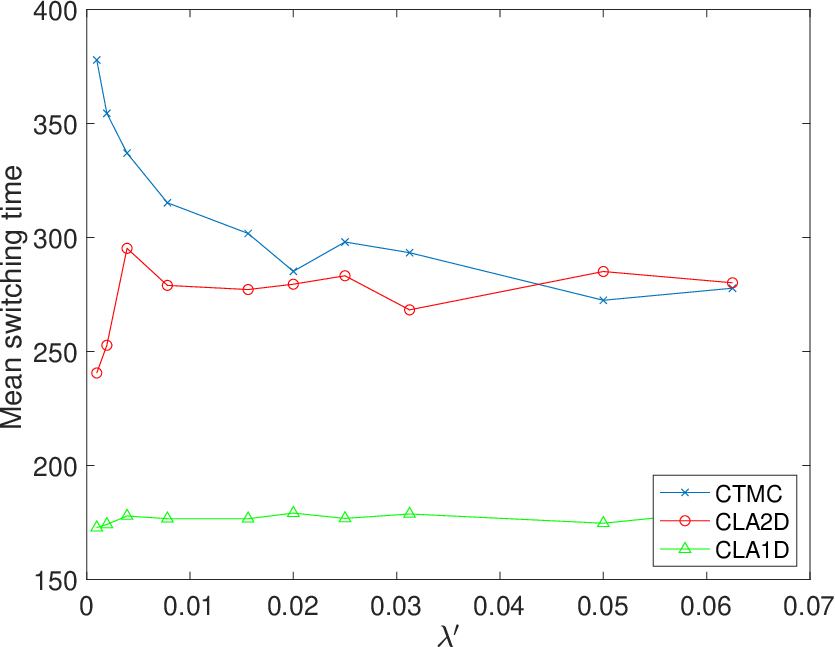
In Figure 3, mean switching time is plotted against different parameters in (7), while fixing other parameters whose value can be found within the caption. Switching time is computed for CTMC (5)-(6) as well as CLA 2D in (8), and the one dimensional reflected approximation in (16), which are termed as CLA 1D in Figure 3.

As $V\rightarrow\infty$ in Figure 3(a), switching time of CTMC can be better approximated by CLA 2D in (8). Such trend can also be observed when $\kappa<1$ in figure 3(b), whereas CLA 1D in 16 become better approximations as $\kappa\rightarrow\infty$. Heuristically as $\kappa\rightarrow\infty$, dynamics of CTMC is dominated by autocatalytic reactions (3), which coincides with the motivation of CLA 1D in (16) where the total mass evolves in a much slower time-scale.

We compare the switching time distributions between the CTMC and the CLA via the histogram in Figure 4. Parameters of the simulation are given by $V=64,\kappa^{\prime}=1$ in (7) for all four figures. In addition, in Figures 4(a)-4(b), $\lambda^{\prime}=\delta^{\prime}=1/32$, as the CTMC in (5)-(6) possess uniform distribution when conditioned on the level sets; in Figures 4(c)-4(d), $\lambda^{\prime}=\delta^{\prime}=1/64$, as the CTMC in (5)-(6) possess bimodal stationary distribution as mass is concentrated on the meta-stable states near the boundary. In both cases, mean and variance of switching time are quite close, and the shape of the distributions is nicely recovered.

However, as $\lambda^{\prime}$ or $\delta^{\prime}\rightarrow 0$, the switching time estimates using CLA 2D (8) are no longer close to the CTMC, as shown in Figure 3(c) and 3(d). In figure 5, such cases were investigated for $V=64,\lambda^{\prime}=\delta^{\prime}=1/256,\kappa^{\prime}=1$, where switching time distribution of CTMC (5)-(6) is approximated by the CLA 1D (16). This approximation yields much better result comparing to CLA 2D in (8), however, the approximation via CLA 1D (16) still underestimates the mean and variance of switching time for the exact CTMC model.

In this section, we first give an explanation on discrepancy between finite time dynamics of 2-dimensional and 3-dimensional TK models. Then we show via simulation that CLA in (8) recovers the stationary distribution of the associated CTMC in (5)-(6). Furthermore we propose cycling time, which is analogous to switching time when $d=2$, and the distribution of cycling time of the CTMC can be well approximated via its associated CLA when $V$ is large.

The main contrast between $d=2$ and $d=3$ for the CTMC, as observed in Figure 1, is that the transition time between meta-stable states for $d=2$ is much longer than that for $d=3$. A heuristic explanation to this is because for 2-dimensional TK model, the two autocatalytic reactions (3) move in opposite directions while sharing the same intensity, hence making it difficult for the process to move between meta-stable states; whereas for higher dimensional TK models ($d\geq 3$), autocatalytic reactions move the process in a cyclic direction, namely $A_{1}\rightarrow A_{2}\rightarrow\cdots\rightarrow A_{d}\rightarrow A_{1}$. More specifically when $A_{1}$ is abundant, dynamics of $A_{1}$ is mainly driven by autocatalytic reactions $A_{d}+A_{1}\rightarrow 2A_{1}$ and $A_{1}+A_{2}\rightarrow 2A_{2}$. However firing of both reactions tend to decrease the rate of $A_{d}+A_{1}\rightarrow 2A_{1}$ and increase the rate of $A_{1}+A_{2}\rightarrow 2A_{2}$, leading to an imbalance toward gaining of $A_{2}$, hence most $A_{1}$ will be changed into $A_{2}$.

Similar to 2-dimensional TK models, positive recurrence are established for $d=3$ in [BKW20], however explicit form of stationary distribution is only derived when $\delta=\frac{3}{2}\kappa$. In figure 6, stationary distribution of the CTMC in (5)-(6) is plotted on the hyperplane $\{x+y+z=3V\}$ for $\delta>\frac{3}{2}\kappa$, $\delta=\frac{3}{2}\kappa$ and $\delta<\frac{3}{2}\kappa$ in row 1. Similar multi-modality of stationary distributions are observed when $\delta<\frac{3}{2}\kappa$. In row 2 of figure 6, stationary distribution of the associated CLA in (8) is plotted via densities near the hyperplane, namely $\left\{|x+y+z-3|\leq\frac{1}{128}\right\}$. In all three cases, the CLA captures the stationary behavior of the exact CTMC model.

As discussed in the different transition time between meta-stable states for $d=2$ and $d=3$, the dominant species when $d=3$ form a cycle, $A_{1}\rightarrow A_{2}\rightarrow A_{3}\rightarrow A_{1}$. Note that such cyclic behavior is not exclusive to parameter regimes when stationary distributions are concentrated near the the boundaries. In figure 7, trajectories of 3-dimensional TK model is plotted for $V=256,\kappa^{\prime}=1$, and $D=\lambda^{\prime}=\delta^{\prime}$ is given by 1/32 and 3/512 respectively. The stationary distribution is unimodal or uniform when conditioning on the hyperplane $\{x+y+z=3V\}$ respectively. In both cases, cyclic behavior still persists within the trajectory, hence we propose cycling time as the analogous quantity in describing finite time dynamics for $d\geq 3$, which can be defined as the second time $X^{3}$ reaches peak abundance when initial condition is given by $(X^{1}_{0},X^{2}_{0},X^{3}_{0})=(0,0,3V)$. Note that the switching time is also well defined in 3-dimensional TK models, however the switching could end up in different regions, i.e. if initially there is only species $A_{3}$, it could move to the boundary with only species $A_{1}$ as well as the boundary with only species $A_{2}$. In comparison cycling time is more straightforward and it consistently captures the average behavior of 3-dimensional TK model.

We will simulate and compare cycling time distribution for the CTMC in (5)-(6) and its associated CLA in (8). In figure 8, mean switching time is plotted against different parameters in (7), while fixing other parameters whose value can be found within the caption. Cycling time is computed for CTMC as well as CLA 3D in (8). Similar to 2D results, mean cycling time is better captured when $V\rightarrow\infty$, or when $\kappa\rightarrow 0$.

In figure 9, cycling time distribution for the CTMC is compared with its associated CLA (8). Simulation of cycling time in figure 9(a)-9(b) is obtained using $V=256,\kappa^{\prime}=1,\lambda^{\prime}=\delta^{\prime}=1/32$, which corresponds to a unimodal stationary distribution. In this case the cycling time distribution of CTMC, as well as its mean and variance, is nicely recovered by its associated CLA.

In figure 9(c)-9(d), We use the same $V$ and $\kappa^{\prime}$, while choosing $\lambda^{\prime}=\delta^{\prime}=3/512$, which corresponds to stationary distribution is uniform when conditioning on the hyperplane. However cycling time distribution associated with CLA underestimates the mean and variance of the cycling time associated to the original CTMC.

In this section, we perform stochastic simulation for higher dimensional TK models. We first give a precise description of 6-dimensional TK model in terms of two switchings: a slow switching between even and odd species, as well as fast switching between dominant regions near the boundary. We then investigate the effect of dimension $d$ on the mean cycling time.

Dynamics of 4-dimensional CTMC (5)-(6) is elaborated in the original publication of [TK01]. In particular, when the system volume $V$ is chosen appropriately (niether too small nor too large) , extinction of species slowly switches between odd and even species in auto-catalytic reaction loop. More precisely, the model switches between states that are abundant in odd species and states that are abundant in even species, during which the other species are almost extinct. Moreover within a temporal domain of abundant odd species, there are fast switches between species $A_{1}$ and $A_{3}$ with large imbalance between the two species, either $X^{1}\gg X^{3}$, or $X^{1}\ll X^{3}$.

To describe the finite time dynamics for $6-$dimensional TK model, we simulate trajectories of the CTMC (5)-(6), with the parameters $V=64,\lambda^{\prime}=\delta^{\prime}=1/256,\kappa^{\prime}=1$. To investigate its switching behavior, we define the process $B(t)$ below that captures the disparity between odd speices and even species:

$\displaystyle B(t)\coloneqq\frac{1}{6V}\sum_{i=1}^{3}(X^{2i-1}(t)-X^{2i}(t)),$

(19)

with initial condition $X^{i}_{0}=V$ for all $i=1,2,\cdots 6$. Exponential convergence to the stationary distribution of CTMC, established in [BKW20], guarantees the denominator $6V$ is approximately the average total population when $T$ is large. Similar expression is considered in [TK01] for 4-dimensional TK model to identify regions of $V$ where discreteness-induced transitions persist.

In figure 10(a), finite time trajectory of $B(t)$ is plotted, and $B(t)$ switches between regions near $B(t)=1$ and $B(t)=-1$, which are regions with abundant odd or even species respectively. Stationary distribution of $B(t)$ is plotted in Figure 10(b) via time averaging, which also yields a bimodal distribution having peaks near $-1$ and $1$.

Next, we investigate the dynamics in between slow switches by analyzing trajectories with abundant odd species. In particular, joint distribution of

$$\left(\rho_{1}(t),\,\rho_{3}(t)\right)=\left(\frac{X^{1}_{t}}{X^{1}_{t}+X^{3}_{t}+X^{5}_{t}},\;\frac{X^{3}_{t}}{X^{1}_{t}+X^{3}_{t}+X^{5}_{t}}\right),$$

conditioning on odd species being abundant, is plotted in figure 11(a) under stationarity via time averaging. Throughout the simulation, the abundance condition is approximated by $B(t)\geq 0.95$. The joint distribution is concentrated within three boundary regions, which can be specified by $\Omega_{i}=\{\rho_{i}\approx 0\}$ for $i=1,3,5$, as each boundary implies one odd species is almost extinct while 2 other odd species are abundant. Moreover these regions are not symmetric with respect to the two dominant species, in the sense that $(\rho_{1},\rho_{3})$ is on average $(0.4,0.6)$ when $\rho_{5}\approx 0$. Such asymmetry exists since the states with more $A_{1}$ is sensitive with respect to the birth of $A_{2}$. More specifically, gaining $A_{2}$ (hence losing $A_{1}$) and losing $A_{2}$ (hence gaining $A_{3}$) is characterized by the autocatalytic reactions $A_{1}+A_{2}\rightarrow 2A_{2}$ and $A_{2}+A_{3}\rightarrow 2A_{3}$, rates of which are completely determined by the relative counts of $A_{1}$ and $A_{3}$. For states with $\rho_{1}\geq\rho_{3}$, higher counts of $A_{1}$ speed up the gaining of $A_{2}$, hence the transition $A_{1}\rightarrow A_{2}\rightarrow A_{3}$ into states with $\rho_{1}\leq\rho_{3}$; on the other hand, states with $\rho_{1}\leq\rho_{3}$ is likely to remain unchanged, since $A_{2}$ is more likely to be exhausted.

In addition to asymmetry, dynamic of odd species, conditioning on odd species being abundant, moves between three dominant regions $\{\Omega_{i}\}_{i=1,3,5}$ in a clockwise manner as plotted in figure 11(a), $\Omega_{5}\rightarrow\Omega_{3}\rightarrow\Omega_{1}\rightarrow\Omega_{5}$. More specifically in the region $\Omega_{5}$ where $A_{5}$ is almost extinct, birth of $A_{4}$ would transition $A_{3}$ into $A_{5}$, which moves the process into the region $\Omega_{3}$. Birth of all other species can not change the dominant molecules of $A_{1}$ and $A_{3}$. Similar movement applies recursively leading to a clockwise cycle in figure 11(a).

To support our claims, a sample trajectory of odd species is plotted in figure 11(b), during which we only have abundant odd species. The process stays within the region $\Omega_{5}$ at time $t=9000$, which switches into the region $\Omega_{3}$ at the time $t=9010$, then proceeds to $\Omega_{1}$ around $t=9020$. At time $t=9025$ the process returns to $\Omega_{5}$ and completed a clockwise cycle.

We summarize the dynamics for $d=6$. Two types of switches can be utilized in describing finite time dynamics of $6-$dimensional TK model when discreteness-induced transitions persist. In particular, abundant molecule species switches between odd and even on a slower time scale. In between these switches, the dynamics dominated by odd species will cycle between boundary regions as $\Omega_{5}\rightarrow\Omega_{3}\rightarrow\Omega_{1}\rightarrow\Omega_{5}$, or $\Omega_{6}\rightarrow\Omega_{4}\rightarrow\Omega_{2}\rightarrow\Omega_{6}$ when the dynamics is dominated by even species.

Last but not least, mean cycling time is plotted against some dimension $d$ in Figure 12. As in previous sections, cycling time is computed for each trajectory as the second time $X^{d}_{t}$ reaches peak abundance (initially there are only species $d$), and mean cycling time are averaged over independent samples. Despite longer cycles as $d$ increases, the cycling time decreases for smaller $d$. This is because if the birth of species $A_{2}$ occurs before the birth of species $A_{1}$, the switches from $A_{d}\rightarrow A_{1}$ and $A_{1}\rightarrow A_{2}$ would happen simultaneously, as it can be observed in Figure 1(c)-1(e)). Such simultaneous switches speed up the cycling and hence reduce the cycling time, whereas these switches are more likely to occur in higher dimensions. However as $d$ increases further, such effect is properly averaged out, and mean cycling time approximately increases linearly in $V$.

Let $\Gamma,\sigma,b,\gamma$ be defined as in (9)-(10), note that $b$ is globally Lipschitz for dimension $d=2$, but only locally Lipschitz for $d\geq 3$ due to the terms $\sum_{k=1}^{d}e_{k}(\kappa^{\prime}(x_{k-1}-x_{k+1})x_{k}$. Precisely,

		$\displaystyle|b(x)-b(y)|$
	$\displaystyle\leq$	$\displaystyle\,\kappa^{\prime}\Big|\sum_{k=1}^{d}e_{k}\Big((x_{k-1}-x_{k+1})x_{k}-(y_{k-1}-y_{k+1})y_{k}\Big)\Big|+\delta^{\prime}\Big|\sum_{k=1}^{d}e_{k}\,(x_{k}-y_{k})\Big|$
	$\displaystyle=$	$\displaystyle\,\kappa^{\prime}\Big|\sum_{k=1}^{d}e_{k}\Big((x_{k-1}-y_{k-1})x_{k}+y_{k-1}(x_{k}-y_{k})\,+\,(x_{k+1}-y_{k+1})x_{k}+y_{k+1}(x_{k}-y_{k})\Big)\Big|+\delta^{\prime}|x-y|$
	$\displaystyle\leq$	$\displaystyle\,2\kappa^{\prime}|x-y|_{\infty}(|x|+|y|)\,+\,\delta^{\prime}|x-y|$
	$\displaystyle\leq$	$\displaystyle\,|x-y|\,\Big(\delta^{\prime}+2\kappa^{\prime}(|x|+|y|)\Big),$

where $|x|=\sqrt{\sum_{i=1}^{d}x_{i}^{2}}$ is the Euclidean norm of $x$, and $|x|_{\infty}:=\max_{1\leq i\leq d}|x_{i}|$.

Note also that $\Gamma(x)$ is symmetric and positive, for all $x\in\mathbb{R}^{d}$. Precisely, for all $x\in\mathbb{R}^{d}_{+}$ and $\theta\in\mathbb{R}^{d}$,

	$\displaystyle\langle\theta,\Gamma(x)\theta\rangle$	$\displaystyle=\sum_{1\leq k\leq d}\left(\lambda^{\prime}+\delta^{\prime}x_{k}\right)\theta_{k}^{2}+\sum_{1\leq k\leq d}\left(\theta_{k}^{2}-\theta_{k}\theta_{k-1}\right)x_{k}x_{k-1}+\sum_{1\leq k\leq d}\left(\theta_{k}^{2}-\theta_{k}\theta_{k+1}\right)x_{k}x_{k+1}$
		$\displaystyle=\sum_{1\leq k\leq d}\left(\lambda^{\prime}+\delta^{\prime}x_{k}\right)\theta_{k}^{2}+\sum_{1\leq k\leq d}\left(\theta_{k}^{2}-\theta_{k}\theta_{k-1}\right)x_{k}x_{k-1}+\sum_{1\leq k\leq d}\left(\theta_{k-1}^{2}-\theta_{k-1}\theta_{k}\right)x_{k-1}x_{k}$
		$\displaystyle=\sum_{1\leq k\leq d}\left(\lambda^{\prime}+\delta^{\prime}x_{k}\right)\theta_{k}^{2}+\sum_{1\leq k\leq d}\left(\theta_{k}-\theta_{k-1}\right)^{2}x_{k-1}x_{k}$
		$\displaystyle\geq\lambda^{\prime}|\theta|^{2}.$		(20)

We can show that $\sigma$ is locally Lipschitz and grows linearly. We note that

	$\displaystyle\|\Gamma(x)\|_{\infty}:=\max_{1\leq i,j\leq d}|\Gamma_{i,j}(x)|$	$\displaystyle\leq\max_{1\leq i\leq d}\kappa^{\prime}(|x_{i-1}|+|x_{i+1}|)|x_{i}|+\lambda^{\prime}+\delta^{\prime}|x_{i}|$
		$\displaystyle\leq 2\kappa^{\prime}|x|_{1}^{2}+\delta^{\prime}|x|_{1}+\lambda^{\prime}.$

So the operator norm on the space of $d\times d$ matrix is of quadratic growth:

$\displaystyle\|\Gamma(x)\|:=\sup_{y\in\mathbb{R}^{d},|y|=1}|\Gamma(x)y|\leq C\left(2\kappa^{\prime}|x|_{1}^{2}+\delta^{\prime}|x|_{1}+\lambda^{\prime}\right)$

for some $C>0$ by the equivalence of norms in $\mathbb{R}^{n}$. Then we have

$\displaystyle\|\sigma(x)\|_{\infty}\leq C\|\sigma(x)\|=C\sqrt{\|\Gamma(x)\|}\leq C^{\prime}\sqrt{\left(2\kappa^{\prime}|x|_{1}^{2}+\delta^{\prime}|x|_{1}+\lambda^{\prime}\right)}.$

Locally Lipschitz of $\sigma(\cdot)$ is given by (20) and the Powers-Stormer inequality [PS70, Lemma 4.2]:

$\displaystyle\|\sqrt{\Gamma(x)}-\sqrt{\Gamma(y)}\|_{HS}\leq\frac{1}{\sqrt{\lambda^{\prime}}}\|\Gamma(x)-\Gamma(y)\|_{HS},$

where $\|\cdot\|_{HS}$ denotes the Hilbert-Schmidt norm. Since all norms are equivalent in finite dimensional vector space and each entry in $\Gamma(\cdot)$ is of second order polynomial, $\Gamma(x)$ is locally Lipschitz, hence $\sqrt{\Gamma(\cdot)}=\sigma(\cdot)$ is also locally Lipschitz.

References

- [AARDVS19] Muhammad Ali Al-Radhawi, Domitilla Del Vecchio, and Eduardo D Sontag. Multi-modality in gene regulatory networks with slow promoter kinetics. PLoS computational biology, 15(2):e1006784, 2019.
- [ABD01] Rami Atar, Amarjit Budhiraja, and Paul Dupuis. On positive recurrence of constrained diffusion processes. Annals of probability, pages 979–1000, 2001.
- [AHLW19] David F Anderson, Desmond J Higham, Saul C Leite, and Ruth J Williams. On constrained langevin equations and (bio) chemical reaction networks. Multiscale Modeling & Simulation, 17(1):1–30, 2019.
- [AK07] Akinori Awazu and Kunihiko Kaneko. Discreteness-induced transition in catalytic reaction networks. Physical Review E, 76(4):041915, 2007.
- [AK11] David F Anderson and Thomas G Kurtz. Continuous time markov chain models for chemical reaction networks. In Design and analysis of biomolecular circuits, pages 3–42. Springer, 2011.
- [BDM14] Tommaso Biancalani, Louise Dyson, and Alan J McKane. Noise-induced bistable states and their mean switching time in foraging colonies. Physical review letters, 112(3):038101, 2014.
- [Ber21] Nils Berglund. Long-time dynamics of stochastic differential equations. arXiv preprint arXiv:2106.12998, 2021.
- [BG11] Thomas Butler and Nigel Goldenfeld. Fluctuation-driven turing patterns. Physical Review E, 84(1):011112, 2011.
- [BGT04] Mireille Bossy, Emmanuel Gobet, and Denis Talay. A symmetrized euler scheme for an efficient approximation of reflected diffusions. Journal of applied probability, 41(3):877–889, 2004.
- [BKW20] Enrico Bibbona, Jinsu Kim, and Carsten Wiuf. Stationary distributions of systems with discreteness-induced transitions. Journal of The Royal Society Interface, 17(168):20200243, 2020.
- [BL07] Amarjit Budhiraja and Chihoon Lee. Long time asymptotics for constrained diffusions in polyhedral domains. Stochastic processes and their applications, 117(8):1014–1036, 2007.
- [BRM12] Tommaso Biancalani, Tim Rogers, and Alan J McKane. Noise-induced metastability in biochemical networks. Physical Review E, 86(1):010106, 2012.
- [CF17] Zhen-Qing Chen and Wai-Tong Louis Fan. Hydrodynamic limits and propagation of chaos for interacting random walks in domains. The Annals of Applied Probability, 27(3):1299–1371, 2017.
- [Che04] Mufa Chen. From Markov chains to non-equilibrium particle systems. World scientific, 2004.
- [DC02] Sever Silvestru Dragomir and Melbourne City. Some gronwall type inequalities and applications. URL: http://rgmia. vu. edu. au/SSDragomirWeb. html, 2002.
- [DH92] JG Dai and J Michael Harrison. Reflected brownian motion in an orthant: numerical methods for steady-state analysis. The Annals of Applied Probability, 2(1):65–86, 1992.
- [DI93] Paul Dupuis and Hitoshi Ishii. Sdes with oblique reflection on nonsmooth domains. The annals of Probability, pages 554–580, 1993.
- [DY56] Evgenii Borisovich Dynkin and Aleksandr Adol’fovich Yushkevich. Strong markov processes. Theory of Probability & Its Applications, 1(1):134–139, 1956.
- [Fan16] Wai-Tong Louis Fan. Discrete approximations to local times for reflected diffusions. Electronic Communications in Probability, 21:1–12, 2016.
- [Gil77] Daniel T Gillespie. Exact stochastic simulation of coupled chemical reactions. The journal of physical chemistry, 81(25):2340–2361, 1977.
- [HLS85] JM Harrison, HJ Landau, and Larry A Shepp. The stationary distribution of reflected brownian motion in a planar region. The Annals of Probability, pages 744–757, 1985.
- [HM19] Linard Hoessly and Christian Mazza. Stationary distributions and condensation in autocatalytic reaction networks. SIAM Journal on Applied Mathematics, 79(4):1173–1196, 2019.
- [HV15] Bahram Houchmandzadeh and Marcel Vallade. Exact results for a noise-induced bistable system. Physical Review E, 91(2):022115, 2015.
- [HW87] J Michael Harrison and Ruth J Williams. Brownian models of open queueing networks with homogeneous customer populations. Stochastics: An International Journal of Probability and Stochastic Processes, 22(2):77–115, 1987.
- [KKP14] Hye-Won Kang, Thomas G Kurtz, and Lea Popovic. Central limit theorems and diffusion approximations for multiscale markov chain models. The Annals of Applied Probability, 24(2):721–759, 2014.
- [Kob11] Tetsuya J Kobayashi. Connection between noise-induced symmetry breaking and an information-decoding function for intracellular networks. Physical review letters, 106(22):228101, 2011.
- [KR14] Weining Kang and Kavita Ramanan. Characterization of stationary distributions of reflected diffusions. The Annals of Applied Probability, 24(4):1329–1374, 2014.
- [KR17] Weining Kang and Kavita Ramanan. On the submartingale problem for reflected diffusions in domains with piecewise smooth boundaries. The Annals of Probability, 45(1):404–468, 2017.
- [KT81] Samuel Karlin and Howard E Taylor. A second course in stochastic processes. Elsevier, 1981.
- [LW19] Saul C Leite and Ruth J Williams. A constrained langevin approximation for chemical reaction networks. The Annals of Applied Probability, 29(3):1541–1608, 2019.
- [MP14] John K McSweeney and Lea Popovic. Stochastically-induced bistability in chemical reaction systems. The Annals of Applied Probability, 24(3):1226–1268, 2014.
- [MT93] Sean P Meyn and Richard L Tweedie. Stability of markovian processes iii: Foster–lyapunov criteria for continuous-time processes. Advances in Applied Probability, 25(3):518–548, 1993.
- [MWHL12] Rui Ma, Jichao Wang, Zhonghuai Hou, and Haiyan Liu. Small-number effects: a third stable state in a genetic bistable toggle switch. Physical review letters, 109(24):248107, 2012.
- [PEO19] Tomislav Plesa, Radek Erban, and Hans G Othmer. Noise-induced mixing and multimodality in reaction networks. European Journal of Applied Mathematics, 30(5):887–911, 2019.
- [PS70] Robert T Powers and Erling Størmer. Free states of the canonical anticommutation relations. Communications in Mathematical Physics, 16(1):1–33, 1970.
- [SA18] Josep Sardanyés and Tomás Alarcón. Noise-induced bistability in the fate of cancer phenotypic quasispecies: a bit-strings approach. Scientific reports, 8(1):1–11, 2018.
- [SAEA18] Josep Sardanyés, Andreu Arderiu, Santiago F Elena, and Tomás Alarcón. Noise-induced bistability in the quasi-neutral coexistence of viral rnas under different replication modes. Journal of The Royal Society Interface, 15(142):20180129, 2018.
- [Sar17] Andrey Sarantsev. Reflected brownian motion in a convex polyhedral cone: tail estimates for the stationary distribution. Journal of Theoretical Probability, 30(3):1200–1223, 2017.
- [SK15] Nen Saito and Kunihiko Kaneko. Theoretical analysis of discreteness-induced transition in autocatalytic reaction dynamics. Physical Review E, 91(2):022707, 2015.
- [SPA05] Michael Samoilov, Sergey Plyasunov, and Adam P Arkin. Stochastic amplification and signaling in enzymatic futile cycles through noise-induced bistability with oscillations. Proceedings of the National Academy of Sciences, 102(7):2310–2315, 2005.
- [TK01] Yuichi Togashi and Kunihiko Kaneko. Transitions induced by the discreteness of molecules in a small autocatalytic system. Physical review letters, 86(11):2459, 2001.
- [TK04] Yuichi Togashi and Kunihiko Kaneko. Molecular discreteness in reaction-diffusion systems yields steady states not seen in the continuum limit. Physical Review E, 70(2):020901, 2004.
- [TM10] Tsz-Leung To and Narendra Maheshri. Noise can induce bimodality in positive transcriptional feedback loops without bistability. Science, 327(5969):1142–1145, 2010.
4 Proofs
This section contains the proofs of the results stated in Section 2. The proofs will be collected in subsection 4.3, after we develop some preliminary estimates for the CLA in subsections 4.1 and 4.2.
4.1 Estimates for the coefficients of CLA
Let be defined as in (9)-(10), note that is globally Lipschitz for dimension , but only locally Lipschitz for due to the terms . Precisely,
where is the Euclidean norm of , and .
Note also that is symmetric and positive, for all . Precisely, for all and ,