- AI
- artificial intelligence
- AoA
- angle-of-arrival
- AoD
- angle-of-departure
- BS
- base station
- BP
- belief propagation
- CDF
- cumulative density function
- CFO
- carrier frequency offset
- CRB
- Cramér-Rao bound
- DA
- data association
- D-MIMO
- distributed multiple-input multiple-output
- DL
- downlink
- EM
- electromagnetic
- FIM
- Fisher information matrix
- GDOP
- geometric dilution of precision
- GNSS
- global navigation satellite system
- GPS
- global positioning system
- IP
- incidence point
- IQ
- in-phase and quadrature
- ISAC
- integrated sensing and communication
- ICI
- inter-carrier interference
- JCS
- Joint Communication and Sensing
- JRC
- joint radar and communication
- JRC2LS
- joint radar communication, computation, localization, and sensing
- IMU
- inertial measurement unit
- IOO
- indoor open office
- IoT
- Internet of Things
- IRN
- infrastructure reference node
- KPI
- key performance indicator
- LoS
- line-of-sight
- LS
- least-squares
- MCRB
- misspecified Cramér-Rao bound
- MIMO
- multiple-input multiple-output
- ML
- maximum likelihood
- mmWave
- millimeter-wave
- NLoS
- non-line-of-sight
- NR
- new radio
- OFDM
- orthogonal frequency-division multiplexing
- OTFS
- orthogonal time-frequency-space
- OEB
- orientation error bound
- PEB
- position error bound
- VEB
- velocity error bound
- PRS
- positioning reference signal
- QoS
- Quality of Service
- RAN
- radio access network
- RAT
- radio access technology
- RCS
- radar cross section
- RedCap
- reduced capacity
- RF
- radio frequency
- RIS
- reconfigurable intelligent surface
- RFS
- random finite set
- RMSE
- root mean squared error
- RTK
- real-time kinematic
- RTT
- round-trip-time
- SLAM
- simultaneous localization and mapping
- SLAT
- simultaneous localization and tracking
- SNR
- signal-to-noise ratio
- ToA
- time-of-arrival
- TDoA
- time-difference-of-arrival
- TR
- time-reversal
- TX/RX
- transmitter/receiver
- Tx
- transmitter
- Rx
- receiver
- UE
- user equipment
- UL
- uplink
- UWB
- ultra wideband
- XL-MIMO
- extra-large MIMO
Radio Localization and Sensing – Part II: State-of-the-art and Challenges
Abstract
This letter is part of a two-letter tutorial on radio localization and sensing, with a focus on mobile radio systems, i.e., 5G and beyond. Building on Part I, which focused on the fundamentals, here we go deeper into the state-of-the-art advances, as well as 6G, covering enablers and challenges related to modeling, coverage, and accuracy.
Index Terms:
Localization, sensing, multipath exploitation.I Introduction
High-performance localization and sensing requires combination of sufficient coverage in terms of infrastructure, resolution of different signal paths, and finally estimation accuracy of the geometric parameters of each resolvable path. Fig. 1 shows different radio technologies, including GNSS and UWB (UWB) [1], in terms of their achievable accuracy for different environments, as well as requirements of selected use cases. With GNSS being limited to outdoors and UWB to short-range applications, 4G, 5G, and 6G provide a bridge. Arguably the main advances towards 5G were the introduction of massive MIMO and the use of mmWave spectrum [2]. Massive MIMO provides high angular resolution [3], but in sub-6 GHz bands still exhibits limited positioning performance, due to the relatively small delay resolution and multipath rich propagation channels. In contrast, mmWave communication (30–300 GHz, though 5G utilizes only lower mmWave bands around 24–53 GHz) has provided unique opportunities for localization, especially when combined with massive arrays, typically analog or hybrid arrays, [4]. In 6G, which is expected to utilize upper mmWave bands (100–300 GHz), with even larger available spectrum, cm-level accuracy is attainable [5].
Let us first review the reasons why 5G and 6G mmWave systems are expected to provide such exceptional performance. First, the use of higher carrier frequencies leads to a more benign propagation channel that is more closely related to the geometry, with a relatively small number of propagation clusters [6, 7]. Second, higher carrier frequencies allow transmission of larger contiguous bandwidths (up to 400 MHz in 5G), providing much better delay resolution than at lower frequencies, where bandwidths are limited to a few tens of MHz. Third, for a fixed physical footprint, a larger number of antenna elements can be fit at the UE (UE) and the BS (BS) sides, enabling fine beamforming and providing enhanced angular resolution. These benefits come at the cost of reduced coverage, sensitivity to blockages and hardware impairments, and higher power consumption than sub-6 GHz deployments.

In parallel, there have been several important developments in communication systems, which provide complementary opportunities for localization and sensing. First, there is the increased importance of ISAC (ISAC), reusing hardware and possibly signals for both sensing and communication functions, with mutual benefits [9]. Second, the deployment of RIS, which are largely passive devices that can modify the propagation environment for improving various KPI [10, 11]. Third, the introduction of other MIMO-based technologies, such as cell-free massive MIMO [12], holographic MIMO [13], and XL-MIMO (XL-MIMO) [14]. Fourth, there are algorithmic advances, such as the use of AI (AI) to tackle certain classes of problems that are hard to solve with model-based methods [15], as well as novel localization and mapping methods [16], analysis tools [17], and signal designs [18].
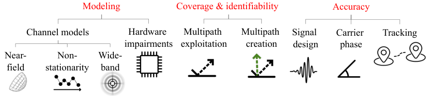
In this letter, we will cover several of these advances, broken down into modeling, enablers for improving coverage and identifiability, and enablers for improving accuracy, as shown in Fig. 2.
II Advances in Modeling
The models from Part I are only valid for a limited operating range. When we go to extremes in terms of bandwidths or array sizes, additional effects should be considered. Moreover, we have ignored the impact of hardware impairments, which will degrade localization and sensing performance.
II-A Radio Channel Models
We recall the channel model from Part I, between a Tx (Tx) with location and a Rx (Rx) with location at frequency (or subcarrier ) and symbol
| (1) |
Suppose path corresponds to an IP (IP) . The steering vector (similarly for ) has entries , where is the location of the -th antenna element, and , all expressed in the Rx frame of reference.
II-A1 Near-Field Propagation
The previous model is in fact a limiting form of a more general model that accounts for wavefront curvature (often called the near-field model) [19], , where is the distance between the source and array’s phase reference, while is the distance between the source and the array’s -th element. Exploiting this wavefront curvature leads to new opportunities to improve accuracy [20], coverage [21], and signal designs [22].
II-A2 Channel Non-stationarity
Non-stationarity refers to the variation of the channel gain across an array and was first observed in XL-MIMO systems [23]. We focus on the LoS (LoS) path in a localization context, where the usual gain expression is [24, Eq. (3)]. Under XL-MIMO conditions, the channel gain depends on the Tx antenna index and the Rx antennas index :
| (2) |
The effect can in principle be decoupled from the wavefront curvature but is often considered jointly. If the channel gain varies significantly as a function of or , conventional localization and sensing methods must be reconsidered, especially the channel parameter estimation routines [25].
(a) Far-field (FF) responses
(b) Near-field (NF) responses
II-A3 Wideband Effects
A final effect we consider pertains to the bandwidth, and is known as beam squint, which is an unfocusing or shifting of beams in an array [26]. Previously, we have used to denote the wavelength, which in fact represents the wavelength at the carrier, . If the signal bandwidth is significant with respect to the carrier, say , then the wavelength becomes frequency-dependent: , where is the subcarrier index and the subcarrier spacing. This wideband effect is especially pronounced for large arrays and should thus be considered together with near-field and non-stationarity effects. When localization or sensing ignores beam squint, significant performance degradation can occur. Hence, dedicated channel parameter estimation routines must be applied [27]. Alternatively, frequency-dependent precoders and combiners, implemented with true time delays can remove beam squint.
II-B Hardware Impairments
Reaching extreme performance requires extreme calibration and puts extreme demands on the communication hardware. Hardware impairments in transceivers can be broken down into synchronization errors (phase noise, clock frequency offsets or drifts, timing errors), array errors (mutual coupling between antenna elements, unknown element responses, array element displacements), and other effects (e.g., power amplifier nonlinearity and quantization) [28]. Synchronization errors are generally time-varying and must thus be tracked and mitigated. Since most localization and sensing methods rely on very precise synchronization as well as measuring phase across time, frequency, and space, synchronization methods must be not only powerful, but also take care of not removing valuable Doppler and phase information. On the other hand, array errors are largely static errors, due to the lack of proper calibration. Hence, these can be learned and mitigated over time. As many of the impairments are nonlinear and dispersive, AI-based methods are well-suited to mitigate them.
II-C Case Study and Analysis Tools
In Fig. 3, we show the antenna responses of a linear array as a function of the azimuth angle and distance, for a 28 GHz system with 64 antennas and 400 MHz bandwidth. The figure shows that the considered effects are all non-negligible, even for these relatively modest parameters. To understand which effect becomes important for a specific localization or sensing problem, the MCRB (MCRB) is a powerful tool [17], as it can lower-bound the performance of the mismatched maximum likelihood estimator [29].
III Improving Coverage and Identifiability
Coverage and identifiability are limited by the BS deployment, but can be improved by multipath exploitation and control, see Fig. 4.

III-A Multipath Exploitation
Multipath exploitation is a generalization of both localization and bistatic sensing of passive objects11 1 This is the common form of multipath exploitation. Alternative approaches rely on RIS or on prior map information, for both monostatic and bistatic configurations., benefiting from the NLoS (NLoS) part of the channel, rather than considering it as a disturbance [30, 31]. By considering each propagation path in (1) as an object, generating a specific ToA (ToA), AoA, AoD (AoD), and Doppler, we can infer the 3D location of IP , e.g., via the relation . Since each multipath component has three spatial degrees of freedom (i.e., ) and a 5-dimensional measurement (ToA, AoA and AoD in azimuth and elevation, if we ignore Doppler), multipath directly contributes to improving localization performance [32]. In Table I, we provide an overview of minimal configurations needed to solve the 3D localization problem (and in the MIMO cases, the 3D orientation problem). Observe that conventionally 4 BSs are needed, while a single BS suffices under multipath exploitation [33]. Finally, note that we have ignored the effect of (i) diffuse multipath (which can be included as part of the noise, though with location-dependent statistics) and (ii) multi-bounce effects, in which case there are several IP per path, where the AoD relates to the first IP and the AoA relates to the last IP, while the ToA depends on the end-to-end propagation distance.
III-B Multipath Creation by RIS
We can also create multipath with the aid of RIS, to improve localization [34] or sensing [35]. An RIS leads to an extra term in the channel (1) of the form
| (3) |
The main difference over (1) lies in the controllable nature of , in which is the complex gain from Tx to RIS, is the complex gain from RIS to Rx, is the RIS response vector, assuming far-field operation, as a function of the AoA from the Tx and the AoD to the Rx . If Tx is a BS, the AoD and AoA are known and do not need to be estimated. The RIS configuration is set by , a diagonal matrix with entries , where is a predetermined set of RIS element configurations that depend on the technology, which may introduce undesired latency. Without amplification, , so that , where is the number of RIS elements. An RIS with known location thus provides a high-dimensional geometric observation (ToA, a 2D angle at the UE, a 2D angle at the RIS and possibly a Doppler) without any additional unknowns. Hence, the RIS acts as a secondary synchronized BS with a phased array, sending the same signal as the real BS. Consequently, as shown in the last row of Table I, a single BS and a single RIS are sufficient to localize a user. The introduction of an RIS does not affect resolvability, as the temporal encoding allows it to be separated from the uncontrolled multipath [34].
| Angle-only SISO | Angle-only MIMO | Angle & delay SISO | Angle & delay MIMO | |
|---|---|---|---|---|
| BS only | not applicable | 2 BS | 4 BS | 2 BS |
| BS + multipath | not applicable | 2 BS | 4 BS | 1 BS, 1 IP [32] |
| BS + multipath, no LOS | not applicable | not identifiable | not identifiable | 1 BS, 4 IP [33] |
| BS + RIS | 1 BS, 2 RIS | 1 BS, 1 RIS | 1 BS, 1 RIS[34] | 1 BS, 1 RIS |
IV Improving Accuracy
Coverage improvements will directly lead to improved accuracy. However, there are additional measures one can take to improve accuracy for any given (optimized [36]) deployment.
IV-A Signal Design
Given the deployment, the system can still optimize the signals sent over the channel, both in terms of time-frequency allocation, as well as through the used transmitter precoders, which we all described by in [24, Eq. (2)]. When there is no a priori location knowledge regarding users/objects, broadcast signals are used, e.g., time-frequency comb pilot signals and an exhaustive sweep of directional beams for positioning and bistatic sensing, or communication-optimal designs with random data for monostatic sensing. As soon as partial information becomes available, it can be used to optimize the signals, applicable for both pilot [18] and data signals [37]. Signal designs can be based on the CRB, with the explicit goal of maximizing accuracy [18]. Given a user with a state uncertainty range and a set of design parameters , then a localization-optimal design is of the form
| (4a) | ||||
| s.t. | (4b) | |||
where the PEB (PEB) was defined in Part I and the constraint ‘’ ensures that the design does not lead to ambiguities in the localization estimates at . To exemplify the design problem, consider the power allocation problem across subcarriers in an OFDM (OFDM) system [38, 39], for performing distance estimation, shown in Fig. 5-(a). The range profiles (correlation output used for maximum likelihood estimation) are shown in Fig. 5-(b). The uniform allocation (in blue) has a broad main peak (about ), but around 13 dB suppression of sidelobes. The red power allocation, which emphasizes the outer subcarriers is thus near-optimal from a PEB perspective with a narrower main peak (about , leading to a PEB reduction of about 60%), but with several strong sidelobes. Hence, the allocation should account for prior information (green and red areas in Fig. 5-(b)) to meet the identifiability constraint.
(a) Power allocation
(b) Range profile (IFFT output)
IV-B Carrier Phase Based Localization
We argued in Part I that in (1) should not directly be used for localization or sensing. In fact, this is only partially true. The phase of (say, ) can be expressed as
where is a phase due to the transmission chain at the Tx and is a phase due to the reception chain at the Rx, is a phase induced by the reflection (for ), and the remainder of is a function of the distance and the carrier frequency. Note that the phase is subject to a ambiguity, . Carrier phase information has two complementary benefits:
- •
- •
Improved resolution: For example, in bistatic sensing, where several widely distributed Tx and Rx are phase-synchronized, an object with location can be resolved with -level resolution [41], providing a way to obtain high resolution with few antennas and limited bandwidth, e.g., at sub-6 GHz frequencies.
IV-C Inference over Time
Localization and sensing accuracy can also be improved by tracking users and objects over time or by fusion with other sensors [42], provided statistical models for the uncertainties are available. Bayesian filtering methods such as the extended Kalman filter are well-suited to this [43]. When UE tracking is combined with multipath exploitation, this is known as SLAM (SLAM),22 2 In particular, as ‘channel SLAM’ or ‘radio SLAM’, as well as ‘5G SLAM’ and ‘mmWave SLAM’. When the objects also move, the problems are referred to as tracking and SLAT (SLAT) while in a pure sensing context it is known as mapping or tracking, which inherently exploits multipath. These problems are often tackled after the range, angle, and Doppler measurements for the resolved paths are obtained. Both SLAM and mapping/tracking are inherently challenging because (i) the number of objects is a priori unknown, objects may not give rise to measurements at each time, while measurements may be due to clutter; (ii) the association between measurements and objects is unknown. Both challenges are elegantly addressed by either BP (BP) [44] or RFS (RFS) theory [16], while performance bounds can be obtained using the posterior CRB [45].
V Outlook towards 6G
With several initiatives worldwide underway to develop the basic building blocks of 6G, several of the models and methods covered in this letter will need to be used. The main trends we see towards 6G are the following:
- 1.
From position to orientation and velocity: Conventional positioning has only considered the 3D location of the UE. 6G will certainly include the 3D UE orientation, as users will have arrays. In addition, to ensure high-SNR operation with long integration types, Doppler and micro-Doppler processing will be beneficial, so that velocity of users and objects can be inferred.
- 2.
Utilizing a variety of carrier frequencies: Much emphasis has been placed on lower and upper mmWave frequencies as main enablers for accurate localization and sensing, but we should not ignore the sub-10 GHz carriers, which provide better energy efficiency and coverage, while resolution can come from wide aperture deployments.
- 3.
The rise of AI: This letter has very much emphasized model-based signal processing. However, in the presence of model uncertainties (as described in Section II) or algorithm deficiencies, data-driven methods can lead to disruptive and powerful designs and algorithms. With increased resolution come opportunities to infer finer details and properties of objects, people, and materials, similar to image processing.
- 4.
ISAC: The use of common hardware and possibly common waveforms for communication and sensing (including localization) will provide important cross-functional benefits, such as reduced overhead beam alignment or radar sensing without dedicated radio emissions.
- 5.
New antenna structures: Both at the user and infrastructure sides, many different antenna and deployment alternatives are being considered for 6G, all of which have implications for localization and sensing. Phase coherence among distributed infrastructure nodes will unlock the ultimate performance, though is very challenging to achieve in practice.
While by no means exhaustive, this short list, along with the models, methods, and challenges highlighted in these letters will hopefully spark new research questions, lead to novel methodologies, and ultimately help achieve the extreme performance demanded by 6G use cases. Based on several decades of experience, we can confidently say that the golden age of radio localization and sensing has only just begun.
References
- [1] M. Z. Win et al., “History and applications of UWB,” Proceedings of the IEEE, vol. 97, no. 2, pp. 198–204, 2009.
- [2] J. G. Andrews et al., “What will 5G be?” IEEE Journal on selected areas in communications, vol. 32, no. 6, pp. 1065–1082, 2014.
- [3] F. Wen et al., “A survey on 5G massive MIMO localization,” Digital Signal Processing, vol. 94, pp. 21–28, 2019.
- [4] O. Kanhere et al., “Position location for futuristic cellular communications: 5G and beyond,” IEEE Communications Magazine, vol. 59, no. 1, pp. 70–75, 2021.
- [5] H. Chen et al., “A tutorial on terahertz-band localization for 6G communication systems,” IEEE Commun. Surveys Tuts., vol. 24, no. 3, pp. 1780–1815, 2022.
- [6] T. S. Rappaport et al., “Overview of millimeter wave communications for fifth-generation (5G) wireless networks—with a focus on propagation models,” IEEE Transactions on antennas and propagation, vol. 65, no. 12, pp. 6213–6230, 2017.
- [7] B. Peng et al., “Channel modeling and system concepts for future terahertz communications: Getting ready for advances beyond 5G,” IEEE Vehicular Technology Magazine, vol. 15, no. 2, pp. 136–143, 2020.
- [8] J. A. del Peral-Rosado et al., “Survey of cellular mobile radio localization methods: From 1G to 5G,” IEEE Communications Surveys Tutorials, vol. 20, no. 2, pp. 1124–1148, 2018.
- [9] F. Liu et al., “Integrated sensing and communications: Towards dual-functional wireless networks for 6G and beyond,” IEEE journal on selected areas in communications, 2022.
- [10] E. C. Strinati et al., “Reconfigurable, intelligent, and sustainable wireless environments for 6G smart connectivity,” IEEE Communications Magazine, vol. 59, no. 10, pp. 99–105, 2021.
- [11] E. Basar et al., “Wireless communications through reconfigurable intelligent surfaces,” IEEE access, vol. 7, pp. 116 753–116 773, 2019.
- [12] Ö. T. Demir et al., “Foundations of user-centric cell-free massive MIMO,” Foundations and Trends® in Signal Processing, vol. 14, no. 3-4, pp. 162–472, 2021.
- [13] C. Huang et al., “Holographic MIMO surfaces for 6G wireless networks: Opportunities, challenges, and trends,” IEEE Wireless Communications, vol. 27, no. 5, pp. 118–125, 2020.
- [14] E. Björnson et al., “Massive MIMO is a reality—what is next?: Five promising research directions for antenna arrays,” Digital Signal Processing, vol. 94, pp. 3–20, 2019.
- [15] T. O’Shea et al., “An introduction to deep learning for the physical layer,” IEEE Transactions on Cognitive Communications and Networking, vol. 3, no. 4, pp. 563–575, 2017.
- [16] H. Kim et al., “PMBM-based SLAM filters in 5G mmwave vehicular networks,” IEEE Transactions on Vehicular Technology, 2022.
- [17] S. Fortunati et al., “Performance bounds for parameter estimation under misspecified models: Fundamental findings and applications,” IEEE Signal Processing Magazine, vol. 34, no. 6, pp. 142–157, 2017.
- [18] M. F. Keskin et al., “Optimal spatial signal design for mmwave positioning under imperfect synchronization,” IEEE Transactions on Vehicular Technology, vol. 71, no. 5, pp. 5558–5563, 2022.
- [19] B. Friedlander, “Localization of signals in the near-field of an antenna array,” IEEE Transactions on Signal Processing, vol. 67, no. 15, pp. 3885–3893, 2019.
- [20] F. Guidi et al., “Radio positioning with EM processing of the spherical wavefront,” IEEE Transactions on Wireless Communications, vol. 20, no. 6, pp. 3571–3586, 2021.
- [21] M. Rahal et al., “RIS-enabled localization continuity under near-field conditions,” in IEEE International Workshop on Signal Processing Advances in Wireless Communications (SPAWC), 2021, pp. 436–440.
- [22] O. Rinchi et al., “Compressive near-field localization for multipath RIS-aided environments,” IEEE Communications Letters, 2022.
- [23] E. De Carvalho et al., “Non-stationarities in extra-large-scale massive MIMO,” IEEE Wireless Communications, vol. 27, no. 4, pp. 74–80, 2020.
- [24] H. Wymeersch et al., “Radio localization and sensing – Part I: Fundamentals,” IEEE Communication Letters, 2022.
- [25] H. Lu et al., “Communicating with extremely large-scale array/surface: Unified modelling and performance analysis,” IEEE Transactions on Wireless Communications, 2021.
- [26] N. J. Myers et al., “InFocus: A spatial coding technique to mitigate misfocus in near-field LoS beamforming,” IEEE Transactions on Wireless Communications, 2021.
- [27] B. Wang et al., “Beam squint and channel estimation for wideband mmwave massive MIMO-OFDM systems,” IEEE Transactions on Signal Processing, vol. 67, no. 23, pp. 5893–5908, 2019.
- [28] A. Mohammadian et al., “RF impairments in wireless transceivers: Phase noise, CFO, and IQ imbalance–A survey,” IEEE Access, vol. 9, pp. 111 718–111 791, 2021.
- [29] H. Chen et al., “MCRB-based performance analysis of 6G localization under hardware impairments,” in IEEE International Conference on Communications (ICC) Workshops, 2022.
- [30] K. Witrisal et al., “High-accuracy localization for assisted living: 5G systems will turn multipath channels from foe to friend,” IEEE Signal Processing Magazine, vol. 33, no. 2, pp. 59–70, 2016.
- [31] S. Wielandt et al., “Indoor multipath assisted angle of arrival localization,” Sensors, vol. 17, no. 11, p. 2522, 2017.
- [32] M. A. Nazari et al., “mmWave 6D radio localization with a snapshot observation from a single BS,” arXiv preprint arXiv:2204.05189, 2022.
- [33] R. Mendrzik et al., “Harnessing NLOS components for position and orientation estimation in 5G millimeter wave MIMO,” IEEE Transactions on Wireless Communications, vol. 18, no. 1, pp. 93–107, 2018.
- [34] K. Keykhosravi et al., “RIS-enabled SISO localization under user mobility and spatial-wideband effects,” IEEE Journal of Selected Topics in Signal Processing, 2022.
- [35] S. Buzzi et al., “Foundations of MIMO radar detection aided by reconfigurable intelligent surfaces,” IEEE Trans. Signal Process., vol. 70, pp. 1749–1763, 2022.
- [36] A. Albanese et al., “LOKO: localization-aware roll-out planning for future mobile networks,” arXiv preprint arXiv:2201.04051, 2022.
- [37] M. F. Keskin et al., “Limited feedforward waveform design for OFDM dual-functional radar-communications,” IEEE Transactions on Signal Processing, vol. 69, pp. 2955–2970, 2021.
- [38] M. Driusso et al., “Performance analysis of time of arrival estimation on OFDM signals,” IEEE Signal Processing Letters, vol. 22, no. 7, pp. 983–987, 2014.
- [39] R. Montalban et al., “Power allocation approaches for combined positioning and communications OFDM systems,” in IEEE Workshop on Signal Processing Advances in Wireless Communications (SPAWC), 2013, pp. 694–698.
- [40] S. Fan et al., “Carrier phase-based synchronization and high-accuracy positioning in 5G new radio cellular networks,” IEEE Transactions on Communications, vol. 70, no. 1, pp. 564–577, 2021.
- [41] A. M. Haimovich et al., “MIMO radar with widely separated antennas,” IEEE Signal Processing Magazine, vol. 25, no. 1, pp. 116–129, 2007.
- [42] X. Guo et al., “A hybrid positioning system for location-based services: Design and implementation,” IEEE Communications Magazine, vol. 58, no. 5, pp. 90–96, 2020.
- [43] M. Koivisto et al., “Joint device positioning and clock synchronization in 5G ultra-dense networks,” IEEE Transactions on Wireless Communications, vol. 16, no. 5, pp. 2866–2881, 2017.
- [44] E. Leitinger et al., “A belief propagation algorithm for multipath-based SLAM,” IEEE transactions on wireless communications, vol. 18, no. 12, pp. 5613–5629, 2019.
- [45] B. Ristic et al., “Comments on ‘Cramér–Rao lower bound for tracking multiple targets’,” IET Radar, Sonar & Navigation, vol. 1, no. 1, pp. 74–76, 2007.