The giants that were born swiftly - Implications of the top-heavy stellar initial mass function on the birth conditions of globular clusters2021The giants that were born swiftly - Implications of the top-heavy stellar initial mass function on the birth conditions of globular clusters–A
Abstract
Recent results suggest that the initial mass function (IMF)of globular clusters (GCs)is metallicity and density dependent. Here it is studied how this variation affects the initial masses and the numbers of core collapse supernovae (CCSNe)required to reproduce the observed iron spreads in GCs. The IMFsof all of the investigated GCswere top-heavy implying larger initial masses compared to previous results computed assuming an invariant canonical IMF. This leads to more CCSNebeing required to explain the observed iron abundance spreads. The results imply that the more massive GCsformed at smaller Galactocentric radii, possibly suggesting in-situ formation of the population II halo. The time until star formation (SF)ended within a proto-GCis computed to be 3.5 - 4 Myr, being slightly shorter than the 4 Myr obtained using the canonical IMF. Therefore, the impact of the IMFon the time for which SFlasts is small.
Keywords:
globular clusters: general – supernovae: general – stars: abundances – methods: analytical1 Introduction
While most globular clusters (GCs)have been observed to be homogeneous with respect to iron (Carretta et al. 2009b; Mucciarelli et al. 2015; Montecinos et al. 2021), there is evidence for iron abundance spreads in some of them (Pancino et al. 2000; Ferraro et al. 2009; Lardo et al. 2016; Marino et al. 2018; Bailin 2019; Lardo et al. 2022). This spread in iron is believed to be caused by pollution through core collapse supernovae (CCSNe), however, it is unclear at which stage of GCdevelopment these CCSNeexploded (D’Antona et al. 2016; Wirth et al. 2021; Lacchin et al. 2021). In Wirth et al. 2021 a novel method to estimate the number of CCSNerequired to explain the iron abundance spread in a GCassuming that the iron spread is caused by CCSNwas introduced. This approach was based on a model in which GCswithout an iron spread arise if star formation (SF)stops before the first CCSNcan pollute the gas in the GC. If SFcontinues past this point, the CCSNewill pollute the surrounding gas with iron, such that more iron rich stars form. Paper I shows how the number of CCSNecontributing to this iron rich population and the time after which SFends can be computed using the iron spread catalogue from Bailin 2019.
An integral part of the calculations in Paper I was to compute the initial masses of the GCs. To this end we used a set of equations which Baumgardt & Makino 2003 derived from N-body simulations. The initial mass of a GCis, like other GCparameters, related to the assumed initial mass function (IMF)(Prantzos & Charbonnel 2006; Marks et al. 2012; Bekki et al. 2017; Jeřábková et al. 2017; Kalari et al. 2018; Schneider et al. 2018; Chon et al. 2021). In Paper I, the canonical IMF(Kroupa 2001; Kroupa et al. 2013) was assumed for all GCs. However, several theoretical (Sharda & Krumholz 2022) and observational (Marks et al. 2012; Zhang et al. 2018; Yan et al. 2021; Pouteau et al. 2022) studies have found that the IMFdoes change depending on the initial density and metallicity of a stellar population.
To determine the IMFof a GCis challenging since the mass function of a GCchanges over time. This is mainly due to two effects: the fact that massive stars die first (Portinari et al. 1998; Marigo 2001, see e.g.) and the loss of stars due to energy-equipartion driven evaporation and ejection (Fall & Zhang 2001; Heggie & Hut 2003; Webb & Leigh 2015). Additionally, mergers can play a role (Kravtsov et al. 2022).
Despite these obstacles, several attempts have been made to compute the IMFof a GC. Only recently, Webb & Bovy 2021 suggested to use the mass function observed at the ends of the tidal tails of a GCto determine the IMF. They do mention, however, that even Gaia will be unable to detect low-mass stars ( for an isochrone and distance of GD-1 and Pal 5) and this does not solve the problem that stars more massive then already evolved off the main sequence (Portinari et al. 1998; Marigo 2001), making them undetectable. As Jerabkova et al. 2021 pointed out, the detection of tidal tails is challenging in general. They suggest a new method, the compact convergent point method, to extract the tidal tails.
Kroupa 2001 combined constrains from different studies into what is known as the canonical IMFand concluded that the existing data may be indicating a systematic variation with metallicity. Kroupa 2002 then formulated evidence for the IMFbecoming more bottom-light (fewer low mass stars) with decreasing iron abundance. Additionally, Marks et al. 2012 found that the slope of the upper end of the IMF(for stars with a mass ) depends on the initial gas cloud density and the iron abundance. They compared a set of numerical simulations to observations to determine the connection between the initial mass function and the properties of the gas clouds the GCsformed out of. Yan et al. 2021 later found a systematic variation in the low-mass part of the IMFas well.
The purpose of this paper is, thus, to investigate how a varying IMFaffects the initial mass computed for the GCsand the number of CCSNerequired to reach the observed spread of . The results of this study will be compared to those in Paper I. Sec. 2 explains how the systematic variation of the IMF, as documented in Yan et al. 2021 is applied to the computation of the initial masses of the GCs. Additionally the method to compute the time after which SFends is explained. Secs. 3 and 4 contain the results and discussion, respectively, and finally we will draw our conclusions in Sec. 5.
2 Methods
2.1 Cluster initial mass as a function of the IMF
In Paper I the results from Baumgardt & Makino 2003 were used to compute the initial stellar mass of the cluster, . Note that this is the mass after revirialisation following a GC’s gas expulsion. Baumgardt & Makino 2003 use the connection between dissolution time, , half-mass relaxation time, , and crossing time, , derived in Baumgardt 2001: . They combine this with the results of their simulations to formulate an equation for the dissolution time of clusters and another one for the evolution of their mass. In Paper I, these findings were combined into one implicit equations that can be solved for numerically:
| (1) |
Note that for consistency the terms are written down in the same order as in Paper I. and are fitting parameters which depend on the King concentration parameter, . is the Coulomb logarithm. and are the apocentre and eccentricity of the GC’s orbit, respectively. is the current mass of the GCand its age. Analogous to Paper I, the age is assumed to be 12 Gyr in accordance with literature values (Dotter et al. 2010; Usher et al. 2019; Cohen et al. 2021). The mean stellar mass and the portion of lost through stellar evolution, , will here be computed depending on the IMF. This is assumed to happen instantaneously (Baumgardt & Makino 2003). Paper I follows Baumgardt & Makino 2003 and assumes , which means that 30% of the initial mass was assumed to be lost due to stellar evolution for an invariant canonical IMF.
2.1.1 Dependence of the IMF on initial cluster mass

The IMF, , is defined through the number of stars born together in the mass interval , . Marks et al. 2012 derived the correlation between the IMF, initial central density and metallicity of a GCby comparing numerical results based on gas-expulsion simulation with observations. Using more recent data, Yan et al. 2021 rewrote the variations in all parts of the IMFas a function of rather than . They formulated the IMF, , as:
| (2) | ||||||
| (3) | ||||||
| (4) | ||||||
| (5) | ||||||
with the initial metallicity of the GC, , and its cloud core density, . is the metal mass fraction in the Sun, is a constant and is a constant assuring the function is continuous and normalized.
Following Forbes et al. 2011, is converted to the total metallicity, , using . The value of is typical for Galactic GCs(Carney 1996; Forbes et al. 2011). The dependency of the IMFon the metalicity and is not arbitrary, but has been extracted from data such that the IMFis consistent with:
- •
direct observational constraints from the Galactic field population and a large range of star clusters (Kroupa 2002; Marks et al. 2012),
- •
the observed dynamical mass-to-light ratios and numbers of low-mass X-ray binary systems in ultra-compact dwarf galaxies (Dabringhausen et al. 2009; Dabringhausen et al. 2012),
- •
the synthesised galaxy-wide IMFsof galaxies of different types (Yan et al. 2017), as well as
- •
galaxy chemical evolution studies (Yan et al. 2021).
All the aforementioned IMF constraints have uncertainties, but the self-consistency-check attained by calculating galaxy-wide stellar populations (Kroupa et al. 1993; Yan et al. 2017; Jeřábková et al. 2018; Yan et al. 2020; Yan et al. 2021) suggests that any true variation is comparable to the above formulation.
Marks & Kroupa 2012 found the following correlation between the density, , and the mass, , of the stars in the still gas embedded clusters by fitting the densities and masses of several datasets (see their fig. 6):
| (6) |
with and . The gas density of the cloud is then , where is the star formation efficiency (SFE). In agreement with Paper I, is assumed (Lada & Lada 2003; André et al. 2014; Megeath et al. 2016; Banerjee & Kroupa 2018, see e.g.). Based on the gas expulsion computations by Brinkmann et al. 2017 it is assumed that a GClooses a negligible fraction of its stars when its residual gas is expelled, i.e. to a good approximation. With these calculations, the IMF can now be expressed in dependence of to and .
Possible forms of the IMFare illustrated in Fig. 1. The canonical IMFis shown by the thick black line. The changes in and depending on are made visible by dashed lines. Additionally, the shape of the IMFfor different are shown. The IMFsbecomes more bottom-light (fewer low mass stars per star formed) with decreasing . Simultaneously, a lower and a higher gas density decrease , making the GCmore top-heavy (more high-mass stars per star formed). We note that this observationally motivated IMFvariation (Eqs. 2 to 5) needs to be further tested, but the variation fulfils the observational constraints from resolved stellar populations and the Galactic field as detailed in Kroupa et al. 2013; Jeřábková et al. 2018; Yan et al. 2021. The deduced top-heavy IMFfor massive GCschanges the dynamical behaviour of the clusters compared to the canonical IMF(Haghi et al. 2020; Mahani et al. 2021; Wang & Jerabkova 2021).
As in Paper I, the IMF was used to compute the mean stellar mass:
| (7) |
where and are the minimum and maximum stellar masses in the GCs, respectively. is computed for each GCby solving eqs. 2 - 4 of Yan et al. 2017, replacing the fixed value of used in Paper I.
2.1.2 Mass lost through stellar evolution

To compute , the life expectancies and remnant masses for stars given in Fig. 2 are used. These were obtained by Yan et al. 2019 by fitting splines (a function defined piecewise as polynomials) to data provided in Portinari et al. 1998 and Marigo 2001. These authors obtained their data from theoretical models. To find the fraction of the initial mass of a GCthat is left depending on its age needs to be computed, neglecting dynamical evolution and thus only focussing on the effects of stellar evolution.
Computing the mass loss of a star over time requires complicated numerical models (Sukhbold et al. 2016; Farrell et al. 2022). However, stars loose most of their mass, after hydrogen burning is over i.e. towards the end of their life (Willson 2000; Heger et al. 2003b). This justifies the simplification used in the present work that all of the mass a star looses is subtracted at the end of its life. It follows then that in a given time interval a GClooses the difference between the initial mass and the remnant mass of all stars dying within this time. The IMFgives us the mass distribution of stars in the GC, with which we can now compute the mass portion of left over in a GCafter accounting for stellar evolution at any given time.
Fig. 3 shows the evolution of the GCmass computed as above for various combinations of , and . As we can see, the majority of a GC’s mass loss through stellar evolution happens before the 1 Gyr mark, while the impact made by dynamical evolution is expected to still be small at this point given the long two body relaxation times. This is no hard boundary and one could easily use or instead. It is worth noting that core collapse happens quicker for GCswith more top-heavy IMFand for GCswith a higher central density. This might be taken into account in future models (Gürkan et al. 2004). The dominance of the mass loss through stellar evolution is consistent with the findings of Baumgardt & Makino 2003 (see their fig. 1), while Joshi et al. 2001 and Lamers et al. 2010 find slightly higher values for the time for which mass loss through stellar evolution dominates (up to ). However, as Fig. 3 shows, the additional mass loss after 1 Gyr is small. The mass of stars dying at this time is around which classify as cool stars. Therefore, this time is used to estimate .
As mentioned below Eq. 1, the mass loss through stellar evolution is assumed to happen instantaneously at the beginning of GCevolution. This is possible since this mass loss dominates with respect to the dynamical mass loss during the GC’s initial evolution, but plays only a small role afterwards (Baumgardt & Makino 2003). A more detailed numerical study of GCsand their mass loss depending on the IMFcan be found in Haghi et al. 2020.
It is worth noting that the mass lost through stellar evolution from the initial population is not added to the remaining gas mass from which the enriched stars form. In the present sample, the mass of the gas returned would have been between and for most GCs. The GCexperiencing the largest gas return is NGC 6441, which would regain 41 % of its initial mass in gas. This would add up to an extra 18 % more gas to the amount of gas to be polluted in Eq. 15. Therefore, gas return can be neglected.
2.1.3 The parameters and
Baumgardt & Makino 2003 fitted and to their Nbody results only for clusters with a King concentration parameter and with and , respectively. However, in this work, and for between 0.7 and 9 is needed, which is the range of we find for the GCsin our sample. Therefore, is computed depending on the initial mass and then extrapolated linearly from the values given above.
To this end the tidal radius, , is calculated as given by eq. 1 of Baumgardt & Makino 2003,
| (8) |
where G is the Newtonian gravitational constant, is the circular velocity of the Galaxy at the coordinates of the GCand the pericentre distance of the GC. As in Paper I, is assumed to be . Additionally, the King radius, , is needed. It is defined in eq. 8.76 of Aarseth et al. 2008,
| (9) | ||||||||
| with | ||||||||
The definition of is taken from Marks & Kroupa 2012. With this the concentration parameter defined as eq. 8.95 in Aarseth et al. 2008 can be computed,
| (10) |
Fig. 8.5 of Aarseth et al. 2008 shows the correlation between and . Fitting a linear curve going through the graph’s origin to the data using the nonlinear least-squares Marquardt-Levenberg algorithm function (Marquardt 1963, see e.g.), the following correlation is obtained:
| (11) |
Interpolating and linearly as mentioned at the beginning of this section leads to:
| (12) | ||||
| (13) |
2.1.4 The resulting numbers of SNe
The number of CCSNe, , needed to produce the observed iron spread is computed analogous to Paper I:
| (14) | ||||
| (15) | ||||
with the mean iron abundance of the GC, , the iron abundance spread, , and the fraction of iron in the Sun, (Asplund et al. 2009). The value of is the average mass of iron released by a CCSNas computed by Maoz & Graur 2017.
2.2 The time after which star formation ends
To compute the time after which SFends, the equations from Paper I need to be adjusted. Firstly, the IMF needs to be integrated to find the number of expected CCSN, , for each GCseparately, instead of having a fixed fraction of the total number of stars as in Paper I:
| (16) |
where is the mass above which stars end their lives as CCSNe. As explained in Sec. 2.1.4, of these CCSNeare required to explain the observed iron spread and, therefore, is the number of CCSNethat contribute to SF. The most massive stars are expected to explode first (Yan et al. 2019, Fig. 2,). This means that the mass, , of the last star to explode in a CCSNwhich still contributes to SFcan be infered from and :
| (17) | ||||
| (18) |
Since is the mass of a star that explodes as a CCSN, it has to be between the minimum mass from which a star becomes a CCSN, , and the maximum stellar mass, computed as explained in Sec. 2.1.1. As in Paper I, the expected lifetime for a star with mass can be looked up in Fig. 2 for , which is close to the -value of most of the GCsin the present sample (Tab. 1). This lifetime is used as the estimate for the time when further SFends.
3 Results
| Name | |||||||||||
|---|---|---|---|---|---|---|---|---|---|---|---|
| 47 Tuc | 8.07 | 5.47 | 7.44 | 1.75 | 27.50 | -0.747 | 0.033 | 3.5 | |||
| NGC 288 | 0.98 | 2.01 | 12.26 | 1.83 | 17.79 | -1.226 | 0.037 | 3.4 | |||
| NGC 362 | 3.36 | 1.02 | 12.41 | 1.65 | 93.75 | -1.213 | 0.074 | 3.5 | |||
| NGC 1851 | 2.81 | 0.85 | 19.20 | 1.61 | 136.44 | -1.157 | 0.046 | 3.4 | |||
| NGC 1904 | 1.56 | 0.82 | 19.51 | 1.62 | 142.09 | -1.550 | 0.027 | 3.5 | |||
| NGC 2419 | 14.30 | 15.89 | 92.20 | 1.78 | 42.97 | -2.095 | 0.032 | 3.5 | |||
| NGC 2808 | 8.69 | 0.97 | 14.76 | 1.61 | 127.73 | -1.120 | 0.035 | 3.4 | |||
| NGC 3201 | 1.41 | 8.20 | 24.15 | 2.00 | 4.32 | -1.496 | 0.044 | 3.4 | |||
| NGC 4590 | 1.32 | 8.95 | 29.51 | 2.06 | 3.72 | -2.255 | 0.053 | 3.4 | |||
| NGC 4833 | 1.80 | 0.90 | 7.68 | 1.67 | 118.88 | -2.070 | 0.013 | 3.5 | |||
| NGC 5024 | 4.17 | 9.11 | 22.21 | 1.92 | 11.69 | -1.995 | 0.071 | 3.4 | |||
| NGC 5053 | 0.73 | 10.33 | 17.74 | 2.12 | 2.20 | -2.450 | 0.041 | 3.4 | |||
| NGC 5139 | 33.40 | 1.33 | 6.99 | 1.62 | 178.36 | -1.647 | 0.271 | 3.5 | |||
| NGC 5272 | 3.60 | 5.44 | 15.16 | 1.88 | 12.17 | -1.391 | 0.097 | 3.5 | |||
| NGC 5286 | 3.59 | 1.17 | 13.32 | 1.72 | 68.41 | -1.727 | 0.103 | 3.4 | |||
| NGC 5466 | 0.55 | 6.80 | 53.55 | 2.10 | 2.07 | -1.865 | 0.075 | 3.4 | |||
| NGC 5634 | 2.20 | 3.97 | 23.76 | 1.94 | 9.09 | -1.869 | 0.081 | 3.4 | |||
| NGC 5694 | 3.67 | 3.90 | 65.74 | 1.91 | 13.10 | -2.017 | 0.046 | 3.4 | |||
| NGC 5824 | 8.49 | 12.48 | 33.72 | 1.85 | 23.77 | -2.174 | 0.058 | 3.5 | |||
| NGC 5904 | 3.68 | 2.89 | 24.03 | 1.83 | 17.63 | -1.259 | 0.041 | 3.4 | |||
| NGC 5986 | 3.31 | 0.70 | 5.08 | 1.56 | 253.81 | -1.527 | 0.061 | 3.4 | |||
| NGC 6093 | 2.64 | 0.36 | 3.53 | 1.38 | 1467.87 | -1.789 | 0.014 | 3.5 | |||
| NGC 6121 | 0.93 | 0.62 | 6.20 | 1.51 | 325.37 | -1.166 | 0.050 | 3.4 | |||
| NGC 6139 | 3.48 | 1.37 | 3.58 | 1.71 | 64.92 | -1.593 | 0.033 | 3.4 | |||
| NGC 6171 | 0.81 | 1.16 | 3.74 | 1.66 | 75.02 | -0.949 | 0.047 | 3.5 | |||
| NGC 6205 | 4.69 | 1.56 | 8.32 | 1.74 | 47.26 | -1.443 | 0.101 | 3.4 | |||
| NGC 6218 | 0.87 | 2.37 | 4.80 | 1.84 | 16.64 | -1.315 | 0.029 | 3.4 | |||
| NGC 6229 | 2.88 | 2.05 | 30.94 | 1.80 | 22.35 | -1.129 | 0.044 | 3.5 | |||
| NGC 6254 | 1.89 | 1.98 | 4.59 | 1.80 | 27.25 | -1.559 | 0.049 | 3.4 | |||
| NGC 6266 | 6.90 | 0.83 | 2.36 | 1.55 | 224.31 | -1.075 | 0.041 | 3.4 | |||
| NGC 6273 | 6.57 | 1.22 | 3.34 | 1.68 | 95.00 | -1.612 | 0.161 | 3.4 | |||
| NGC 6341 | 3.12 | 1.00 | 10.57 | 1.71 | 92.11 | -2.239 | 0.083 | 3.5 | |||
| NGC 6362 | 1.16 | 2.54 | 5.16 | 1.84 | 15.32 | -1.092 | 0.017 | 3.4 | |||
| NGC 6366 | 0.43 | 1.97 | 5.31 | 1.79 | 17.45 | -0.555 | 0.071 | 4.9 | |||
| NGC 6388 | 11.30 | 1.11 | 3.78 | 1.59 | 110.26 | -0.428 | 0.054 | 4.2 | |||
| NGC 6397 | 0.90 | 2.63 | 6.23 | 1.91 | 12.37 | -1.994 | 0.028 | 3.5 | |||
| NGC 6402 | 7.39 | 0.63 | 4.36 | 1.50 | 362.45 | -1.130 | 0.053 | 3.4 | |||
| NGC 6441 | 12.50 | 1.00 | 3.91 | 1.57 | 126.76 | -0.334 | 0.079 | 5.9 | |||
| NGC 6535 | 0.13 | 0.97 | 4.50 | 1.68 | 103.20 | -1.963 | 0.035 | 3.5 | |||
| NGC 6553 | 4.45 | 1.26 | 2.32 | 1.66 | 49.39 | -0.151 | 0.047 | 6.3 | |||
| NGC 6569 | 2.28 | 1.88 | 2.97 | 1.73 | 36.03 | -0.867 | 0.055 | 3.6 | |||
| NGC 6626 | 2.84 | 0.58 | 2.89 | 1.49 | 452.45 | -1.287 | 0.075 | 3.4 | |||
| NGC 6656 | 4.09 | 2.95 | 9.48 | 1.86 | 19.75 | -1.803 | 0.132 | 3.4 | |||
| NGC 6681 | 1.20 | 0.85 | 4.93 | 1.62 | 149.57 | -1.633 | 0.028 | 3.5 | |||
| NGC 6715 | 16.20 | 12.50 | 36.59 | 1.74 | 50.19 | -1.559 | 0.183 | 3.5 | |||
| NGC 6752 | 2.32 | 3.23 | 5.37 | 1.87 | 14.72 | -1.583 | 0.034 | 3.4 | |||
| NGC 6809 | 1.88 | 1.59 | 5.54 | 1.79 | 36.99 | -1.934 | 0.045 | 3.5 | |||
| NGC 6838 | 0.63 | 4.75 | 7.08 | 1.95 | 4.46 | -0.736 | 0.039 | 3.8 | |||
| NGC 6864 | 4.10 | 1.80 | 17.51 | 1.76 | 33.22 | -1.164 | 0.059 | 3.5 | |||
| NGC 7078 | 4.99 | 3.57 | 10.40 | 1.88 | 19.26 | -2.287 | 0.053 | 3.5 | |||
| NGC 7089 | 5.20 | 0.56 | 16.93 | 1.50 | 417.15 | -1.399 | 0.021 | 3.5 | |||
| NGC 7099 | 1.39 | 1.49 | 8.17 | 1.82 | 35.18 | -2.356 | 0.037 | 3.5 | |||
| Terzan 1 | 2.72 | 0.24 | 1.48 | 1.22 | 5089.44 | -1.263 | 0.037 | 3.4 | |||
| Terzan 5 | 7.60 | 0.89 | 2.96 | 1.56 | 136.44 | -0.092 | 0.295 | - | |||
| Terzan 8 | 0.58 | 0.24 | 1.65 | 1.29 | 4604.79 | -2.255 | 0.098 | 3.5 |
The results calculated for a top-heavy IMFare compiled in Tab. 1. As in Paper I the metallicities cited were taken from Bailin 2019 and the present day GCmasses and orbital parameters are taken from Hilker et al. 2019. Note that an upgraded catalogue for the metallicities is available (Bailin & von Klar 2022), however, for consistency with Paper I the old version (Bailin 2019) is used for this work. The data in Table 1 show that the obtained values for the mass function index, , are all smaller than and, therefore, the IMFis more top-heavy than the canonical IMFfor all of the GCs. In the following sections the individual properties and how they compare to the results in Paper I will be discussed. The results from Paper I are marked with a superscript ‘’ (to stand for canonical).
3.1 The initial masses
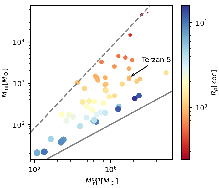


In Figs. 4 to 8 limiting functions were fitted to the data. The method for obtaining these functions is described in Appendix A. The code to fit these functions can be found on the authors’ github repository11 1 https://github.com/Henri-astro/LimiFun.
In Fig. 4 the new results computed using a variable IMF, , are compared with the computed using the canonical IMF(Paper I). The differences between and sensitively depend on the assumed IMF variation law, that is, Eqs. 2 to 5. For small the increase of compared to is larger. That means that GCswith more top-heavy IMFsloose mass more rapidly than GCswith larger . This is in agreement with Baumgardt et al. 201922 2 Note that in Baumgardt et al. 2019 the IMF power-law indices, , are defined with the opposite sign.. However, while Baumgardt et al. 2019 conclude that the combined mass of all early GCsin the Galaxy must have been some , according to the present study calculations the 55 GCsin our sample already exceed this mass. Part of the reason is the higher maximum stellar mass in this work. Baumgardt et al. 2019 used only for all of their GCs, while in this study the --relation found by Yan et al. 2017 is used. With this, values for between 140 and are found for the GCsstudied here. Consequently, in the most massive GCsstudied here up to 80 % of the initial mass is in stars more massive than .
Another question the top-heavy IMFleads to is, how many stars can form in a GCbefore star formation is suppressed due to the heating of the gas. Several studies showed that stellar winds and radiation can disperse the gas in a stellar cluster before the first CCSNeoccur (Lada & Lada 2003; Dale et al. 2012; Verliat et al. 2022). The overabundance of massive stars relative to the canonical IMFwould increase these effects and could eventually prevent iron-enhanced stars from forming. However, further investigation is required to estimate the exact magnitude of these effects depending on the IMFand the birth gas density, and .
As expected from Eqs. 4 and 6 and visible in Fig. 4, increases with decreasing . Since is below the value for the canonical IMFfor all GCs, is always larger than . The difference between and increases with decreasing . This is partly because the tidal radius computed using Eq. 8 is the tidal radius of the GCat its pericentre. This means that the mass loss for low--GCsis stronger, which means that their initial masses were larger and therefore their is increased. A similar but weaker correlation can be found, if a similar plot is done with , as defined below Eq. 1, instead of . This leads to the conclusion that the difference between based on a top-heavy IMFcompared to based on a canonical IMFis larger for GCscloser to the Galactic centre.
The smaller is for a GC, the stronger is the tidal force from the Galactic gravitational field it is exposed to. This means that the dissolution times for GCsget smaller with decreasing . Therefore, if a GCcomes close enough to the Galactic centre, its dissolution time becomes smaller than the age of the present day GCs, (Dotter et al. 2010; Usher et al. 2019; Cohen et al. 2021). As visible in Figs. 4 and 5, there is a lack of low--GCsat the lower end of . The lower limit for not yet dissolved GCsis found at:
| (19) |
That this is the lower limit for undissolved GCsis further supported by the fact that the present-day masses of the GCsget smaller for GCscloser to the boundary. It is, however, likely for these GCsto still exist as dark clusters to this day (Banerjee & Kroupa 2011). Furthermore, there appears to be a lack of distant initially massive GCs. This is even more visible in Fig. 6, which shows over the mean orbital distance over time, (Stein 1977). This would suggest that more massive GCsformed preferably near the Galactic centre (small ). In Fig. 7 it is shown that this result holds even if the canonical IMFis used, which indicates that this result is robust.
It is important to note that in both this work and in Baumgardt & Makino 2003, was used to compute the tidal radius (see Sec. 2.1.3). is the smallest distance the GCcan have from the Galactic centre. This leads to an underestimate of the tidal radius and therefore an overestimate of the mass loss of a GC. This overestimation is larger for larger eccentricities, since the orbit of a GCwith large eccentricity deviates more from a circular orbit with radius . As visible in Fig. 6 the GCsclose to the lower boundary (lower grey line) all have very low eccentricities, therefore, the values are expected to be close to the real ones. However, the GCsclose to the upper boundary (upper grey line) all have high eccentricities, indicating that we are likely to have overestimated their masses. To determine the actual extent of this overestimate, the simulations of Baumgardt & Makino 2003 would have to be rerun with more precise estimates of the tidal radius. 47 Tuc is an outlier when it comes to the eccentricity and has been labelled in both Figs. 6 and 7.
3.2 The number of SNe and the time SF ends

One of the key results of Paper I was that the number of CCSNeper unit mass required to reproduce the observed metal-enrichment, , is independent of . Therefore, does not change between this work and Paper I (compare Tab. 1 and tab. 1 in Paper I). However, the change in propagates through to in the form . This leads to the behaviour visible in Fig. 8, which is similar to that for in Fig. 4. The difference between and is larger for GCscloser to the Galactic centre.
As in Paper I, the number of CCSNerequired to produce the iron spread observed in Terzan 5 is larger than . This leads to the conclusion that Terzan 5 must have been formed through a different scenario, like for example a merger (Massari et al. 2014, Paper I). GCswith unusual chemical compositions can also form through the merger of two chemically distinct molecular clouds (Han et al. 2022). Terzan 5 has been marked in all relevant figures.


In Fig. 9 the time when SFends is plotted over and compared to our data from Paper I. Note that Terzan 5 is missing, since the required number of CCSNeexceeds the number of CCSNeexpected for this GC(see Tab. 1). This makes it impossible to compute . The calculated times until SF ends depend on the assumed lifetime of massive stars (Fig. 2). Different stellar evolution models can result in different lifetimes with uncertainties of a few Myr. The increase of discussed in Sec. 3.1 is clearly visible in this plot. Additionally, the time until SFends is reduced significantly. This is because GCswith top-heavy IMFsproduce a larger fraction of their CCSNeearly on due to the larger fraction of massive stars. The times until SFends obtained here are in agreement with the times after which GCshave been observed to be free of gas (Bastian & Strader 2014) and with theoretical models concerning the timescales with which gas is expelled from GCsvia CCSNe(Calura et al. 2015).
Similar to Fig. 9, Fig. 10 shows the time until SFends, however, this time in the form of a histogram. It is clearly visible that is shorter using a top-heavy IMFcompared to the results of our calculations using a canonical one. For most GCs, SFends after . As for the results computed with the canonical IMF, this is in agreement with studies showing that the GCsand young massive clusters are gas free after at most (Calura et al. 2015; Krause et al. 2016).
The correlation between the mean iron abundance and the time until SFends observed in Paper I is also apparent in our data (Fig. 9) with a variable IMF. However, as in Paper I, this might be due to an underestimate of the error of the iron spread, which would increase the calculated number of CCSNepreferentially for GCswith large mean iron abundances. Therefore, it is unclear whether or not this is a physical effect. According to Marks et al. 2012, a higher mean iron abundance is expected to lead to a less top-heavy IMF. Therefore, the portion of massive stars would be lower, which would lead to fewer CCSNeearly on in GCevolution. This means that it is expected that gas is driven out more slowly leading to a larger , which would support the result we observe in Fig. 9.
4 Discussion
4.1 The upper mass limit of GCs
As stated in Sec. 3.1, the upper initial mass limit of GCsdecreases with increasing distance from the Galactic centre. The same has been observed by Pflamm-Altenburg et al. 2013 for young star clusters around M33. They suggested that this would be due to higher gas surface densities (more material) in the inner regions of galaxies.
The star clusters in M33 are very young (Sharma et al. 2011; Pflamm-Altenburg et al. 2013, ,) and, therefore, the mass loss experienced by these clusters is expected to be small (, with the current cluster mass ). Pflamm-Altenburg et al. 2013 expressed the mass of the most massive clusters in their radially binned sample as a function of their current galactocentric distance, , using the following expression:
| (20) |
By fitting this function to the data from the clusters in M33, they found that the clusters with the highest mass roughly followed the function with and . To obtain their fit they distributed their clusters into bins of 17 clusters each depending on their radial distance to the centre of M33. They then used the - and -values of the most massive clusters in each bin to obtain their fit. In this work, the maximum GCmass is fitted using the method explained in App. A and which lead to as the upper boundary (see Fig. 6). This means that the upper limits of the initial masses of the GCsin our Galaxy are about three orders of magnitude higher than the ones in M33. Note, however, that in both cases the sample size is too small to reliably determine the shape of the radial upper limit function.
While both, M33 and the very young Galaxy have their newly-formed, most massive cluster masses decrease systematically with the galactocentric radius, the two cases are very different: M33 is a late-type disk galaxy about ten times less massive than the Galaxy (Corbelli 2003; McMillan 2011; Kafle et al. 2012; McMillan 2017), is on the galaxy main sequence and is forming open star clusters, while the GC system studied here consists of 12 Gyr old GCsin the Galactic halo. Since the mean GCmass increases with the mass of the host galaxy (Harris et al. 2013) we expect differences in the maximum mass function for those two systems.
4.2 Consequences for the Galaxy
Assuming the Galaxy and all GCswere also formed in-situ (Gilmore & Wyse 1998), eqs. 9 - 12 from Yan et al. 2017 can be used to compute the star formation rate (SFR)of the Galaxy at the time the GCswere forming. With a maximum GCmass of for Terzan 1 we compute a SFRof . This is about 100 times higher than the mean SFRof the Galaxy and could be due to SFRfluctuations, or due to the most massive GCshaving a different origin. It is, however, worth mentioning that especially for massive GCs, like Cen and Terzan 5, alternative formation scenarios, such as mergers or being the remnant of a tidally thrashed dwarf galaxy, have been proposed (Bekki & Freeman 2003; Massari et al. 2014; Marks et al. 2022, see e.g.). If the real maximum GCmass was, for example, only half as large, the SFRbecomes . If the three most massive GCs() of the sample are excluded, less than a tenth of the maximum GCmass used above is needed. The resulting SFRis only .

As visible in Fig 11 the closer a GCis to the Galactic centre, the larger the mass fraction it lost with respect to its initial mass. This is a direct consequence of the results of the numerical experiments by Baumgardt & Makino 2003. Contrary to this, Bastian & Lardo 2015 concluded, based on a lack of a connection between the radial distance of a GCto the Galactic centre and the fraction of enriched stars within it, that no radial dependency between the cluster mass loss and its coordinates exists. They expect a radial dependency to exist due to a preferential loss of 1st generation stars which are known to be less concentrated. In a stronger tidal field they should, therefore, be lost faster and their present day fraction in the GCshould be lower. Bastian & Lardo 2015 define first-generation stars as those with sodium abundance, , between and . The minimum sodium abundance, , of a GCwas determined by eye from --plots of the GCsexcluding outlying stars. However, Marino et al. 2019 find that in many GCsthe difference between first and second generation is smaller than this. In fact, the -values of 1st and second generation stars overlap in some of the cases.
Bastian & Lardo 2015 used present-day fractions of enriched stars from a number of studies (Carretta et al. 2009a; Carretta et al. 2011; Carretta et al. 2012; Carretta et al. 2013; Kacharov et al. 2013; Carretta et al. 2014; Carretta et al. 2015; Marino et al. 2015). Fig. 11 is colourcoded according to the data collected by Bastian & Lardo 2015. This figure confirms that there is indeed no obvious correlation between the fraction of enriched stars, , and the GC’s distance from the Galactic centre or the mass fraction remaining. However, due to the large number of datasets used, the unreliable boundary between different generations and the large scatter, this is not conclusive evidence against a preferential mass loss nearer to the Galactic centre.
The higher initial masses of the GCswould imply that a larger portion of the stars in the Galactic halo originated from GCs. The mass of the stellar halo is currently estimated to be up to (Deason et al. 2019). Note, however, that this estimate was made using the canonical IMFfrom Gaia measurements of red giants in the halo. A top-heavy galaxy-wide IMFwould increase the initial halo mass significantly. Additionally, the number of stellar remnants would be increased (Yan et al. 2021). These remnants would either stay inside the GCor be expelled due to dynamical processes, remaining as free-floates in the halo (Baumgardt et al. 2008). In our sample the number of neutron stars and black holes is on average 36 times higher than when assuming a canonical IMFfor all GCs. The most extreme case in this study, Terzan 8, produces 403 times as many neutron stars and black holes as it would with a canonical IMF.
4.3 Improvements for future models
Since a modified version of the method applied in Paper I is used, most of the limitations discussed in sec. 4.2 of Paper I apply in this work as well. Among them is the possibility of failed CCSNe(Pejcha & Thompson 2015; Sukhbold et al. 2016; Basinger et al. 2020; Neustadt et al. 2021), in which case some massive stars would end their lives without contributing any iron. This would lead to longer timespans until SFends, which is also discussed in Renzini et al. 2022.
The dependence of the iron output on the CCSNmass was also neglected. However, it is likely, that the amount of ejected iron does depend on the mass of the progenitor. From the short timespan after which SFends (Fig. 9), it follows that only the most massive stars contribute to the iron available for the formation of further stars. Therefore, if for example, the most massive stars would contribute twice as much iron as the average CCSN, only half as many CCSNewould be required and the time until SFends would become shorter. Calculations by Nomoto et al. 2013 show that, for example, a -star with an initial metallicity of alone can produce in iron. An important upgrade for our model in the future would therefore be to use more detailed CCSNeyield models to more accurately compute the number of CCSNeneeded to explain the observed iron spreads. Additionally, supernovae 1a can happen early as edge-lit type 1a SNe (Regős et al. 2003). This has also be neglected.
As shown in Paper I possible errors in measurements of have a significant influence on the result. In appendix A of Paper I it is shown that an overestimate of the measurement errors for individual stars in the sample by 0.13 dex can lead to an overestimate of the CCSNerequired by over 1 dex. Similarly, errors in the mean for a GC, which might occur as a result of over- or underestimating the sizes of the different stellar populations within the GCs, can lead to over and underestimates in the number of CCSNerequired to explain the iron spread. Since the iron spread is given in dex, it’s value in absolute numbers depends on the value of (see Eq. 15). An underestimate of would lead to an underestimate of the number of CCSNerequired and vice versa. For example an underestimate of by 0.1 would lead to a 20% underestimate of the number of CCSNerequired.
One of the main assumptions of our model, not discussed thus far, is that the GCsmove on constant Keplerian orbits. However, various effects like encounters with other GCs, gas clouds and dynamical friction could have altered the orbits of the GCs. If the GCsused to be further away then mass loss would also be reduced, which means that we have overestimated . The orbital evolution of GCscould be determined by ‘backwards-integrating’ the paths of all GCsin the Galaxy as in Portegies Zwart & Boekholt 2018, though this would not cover interactions with GCsor molecular clouds that are already dissolved or unknown. The model of Baumgardt & Makino 2003 would have to be expanded to integrate over the orbital path rather than assuming a constant orbit.
Furthermore, a constant SFEof 0.3 is assumed for each GC. In the current model a higher (lower) SFEwould lead to a lower (higher) fraction of the gas being left over, which means that less (more) iron was needed to be produced. For a constant gas cloud mass before SF, the mass of iron required, , is proportional to . Because of this, would increase for a smaller SFE. While the value of the SFEis still unclear, Ashman & Zepf 2001 suggested that the SFEmight vary with the density of the molecular cloud the GCforms out of. From Eq. 4 we see that a higher density leads to a more top-heavy IMF, which would lead to more CCSNeexpected to explode early on, ensuring a self-regulation of the formation of a GC.
Another pressing question to answer, is how to form new stars in a gas cloud already densely populated by stars, that heat the gas. Parmentier et al. 1999 suggested that the second generation of stars would form in the shock waves caused by CCSNe. This would be in agreement with the present findings, however, it would also mean that the assumption of well-mixed gas in our model would need to be revisited.
5 Conclusions
In this work the initial masses and numbers of CCSNerequired to explain the iron abundance spreads of 55 Galactic GCsis investigated. Based on the assumption that the gas cloud a GCforms out of is well mixed (has the same mean iron abundance at every point in space) and that it is polluted by CCSNeinstantaneously, an analytical model is used. The stars are assumed to form with the systematically variable IMFin accordance with Yan et al. 2021, while the initial masses of the GCsare deduced considering stellar evolution as well as the dynamical mass loss of the star clusters, using the algorithm described in Baumgardt & Makino 2003.
The main results of this work summarize as follows:
- (1)
The initial masses of the GCscomputed allowing for the metallicity and density dependent IMFare larger than the ones calculated using the canonical IMF(Paper I) by a factor of up to . This also increases the number of CCSNerequired to explain the observed iron abundance spreads, as more iron needs to be produced to pollute the more massive gas cloud.
- (2)
The computed mass function power-law index for high-mass stars () is smaller than 2.3 for all GCs, which means that all GCshad IMFsthat were more top-heavy than the canonical one. This decreases the time until SFends since the fraction of massive stars is larger and therefore a larger portion of the CCSNeare from massive, short-lived stars (Dabringhausen et al. 2012). According to our model, for the majority of Galactic GCswithin the studied sample, the SFended after 3.5 to 4.0 Myr after their birth. A larger portion of massive stars would also mean that the number of neutron stars and black holes created from the cluster stars is increased. In the present study we find on average 36 times as many neutron stars (NSs)and black holes (BHs)being formed compared to the results assuming a canonical IMFfor all GCs. The most extreme case in this study, Terzan 8, produces 403 times as many neutron stars and black holes than it would with a canonical IMF.
- (3)
Both the lower and the upper limit for the initial GCmass is largest close to the Galactic centre and declines with the Galactocentric radius. The first finding is easily explained as GCsnear the Galactic centre dissolve quicker due to the stronger gravitational field. The second finding points towards more massive GCshaving formed closer to the Galactic centre than further away (Pflamm-Altenburg et al. 2013, see also). To determine if this is a general trend for GCmasses within galaxies, more GCsystems need to be analysed. This would give us valuable information to determine whether or not GCswere formed in-situ and thus during the earliest assembly phase of the Galaxy with implications for the formation of super-massive black holes (Kroupa et al. 2020). The monolithic-collapse-model for the formation of galaxy spheroids, bulges and elliptical galaxies implies that the most massive clusters form in the innermost regions of the later galaxy. These can appear as quasars (Jeřábková et al. 2017). In this model, the mass of the most-massive central star cluster correlates with the mass of the final galaxy. While the formation of the galaxy occurs on the down-sizing time, the central star cluster’s stellar black holes are compressed into a relativistic state by the in-falling gas. They form, within a few hundred Myr, a super-massive black hole through gravitational-wave-emission-driven collapse of the central stellar-black-hole system (Kroupa et al. 2020).
Acknowledgements
We want to thank an anonymous referee for their useful comments. The authors acknowledge support from the Grant Agency of the Czech Republic under grant number 20-21855S and through the DAAD-Eastern-Europe Exchange grant at Bonn University. Z.Y. acknowledges support from the Fundamental Research Funds for the Central Universities under grant number 0201/14380049. Z.Y. acknowledges support through the Jiangsu Funding Program for Excellent Postdoctoral Talent under grant number 20220ZB54. Z.Y. acknowledges the support of the National Natural Science Foundation of China (NSFC) under grants No. 12041305 and 12173016. Z.Y. acknowledges the science research grants from the China Manned Space Project with NO.CMS-CSST-2021-A08 (IMF).
Data availability
The data used here has been cited and is available in published form.
References
- Aarseth et al. (2008) Aarseth S. J., Tout C. A., Mardling R. A., 2008, The Cambridge N-Body Lectures. Vol. 760, doi:10.1007/978-1-4020-8431-7,
- André et al. (2014) André P., Di Francesco J., Ward-Thompson D., Inutsuka S. I., Pudritz R. E., Pineda J. E., 2014, in Beuther H., Klessen R. S., Dullemond C. P., Henning T., eds, Protostars and Planets VI. p. 27 (arXiv:1312.6232), doi:10.2458/azu_uapress_9780816531240-ch002
- Ashman & Zepf (2001) Ashman K. M., Zepf S. E., 2001, AJ, 122, 1888
- Asplund et al. (2009) Asplund M., Grevesse N., Sauval A. J., Scott P., 2009, ARA&A, 47, 481
- Bailin (2019) Bailin J., 2019, ApJS, 245, 5
- Bailin & von Klar (2022) Bailin J., von Klar R., 2022, ApJ, 925, 36
- Banerjee & Kroupa (2011) Banerjee S., Kroupa P., 2011, ApJ, 741, L12
- Banerjee & Kroupa (2018) Banerjee S., Kroupa P., 2018, Formation of Very Young Massive Clusters and Implications for Globular Clusters. p. 143, doi:10.1007/978-3-319-22801-3_6
- Basinger et al. (2020) Basinger C. M., Kochanek C. S., Adams S. M., Dai X., Stanek K. Z., 2020, arXiv e-prints, p. arXiv:2007.15658
- Bastian & Lardo (2015) Bastian N., Lardo C., 2015, MNRAS, 453, 357
- Bastian & Strader (2014) Bastian N., Strader J., 2014, MNRAS, 443, 3594
- Baumgardt (2001) Baumgardt H., 2001, MNRAS, 325, 1323
- Baumgardt & Makino (2003) Baumgardt H., Makino J., 2003, MNRAS, 340, 227
- Baumgardt et al. (2008) Baumgardt H., Kroupa P., Parmentier G., 2008, MNRAS, 384, 1231
- Baumgardt et al. (2019) Baumgardt H., Hilker M., Sollima A., Bellini A., 2019, MNRAS, 482, 5138
- Bekki & Freeman (2003) Bekki K., Freeman K. C., 2003, MNRAS, 346, L11
- Bekki et al. (2017) Bekki K., Jeřábková T., Kroupa P., 2017, MNRAS, 471, 2242
- Brinkmann et al. (2017) Brinkmann N., Banerjee S., Motwani B., Kroupa P., 2017, A&A, 600, A49
- Calura et al. (2015) Calura F., Few C. G., Romano D., D’Ercole A., 2015, ApJ, 814, L14
- Carney (1996) Carney B. W., 1996, PASP, 108, 900
- Carretta et al. (2009a) Carretta E., et al., 2009a, A&A, 505, 117
- Carretta et al. (2009b) Carretta E., Bragaglia A., Gratton R., D’Orazi V., Lucatello S., 2009b, A&A, 508, 695
- Carretta et al. (2011) Carretta E., Lucatello S., Gratton R. G., Bragaglia A., D’Orazi V., 2011, A&A, 533, A69
- Carretta et al. (2012) Carretta E., Bragaglia A., Gratton R. G., Lucatello S., D’Orazi V., 2012, ApJ, 750, L14
- Carretta et al. (2013) Carretta E., et al., 2013, A&A, 557, A138
- Carretta et al. (2014) Carretta E., et al., 2014, A&A, 564, A60
- Carretta et al. (2015) Carretta E., et al., 2015, A&A, 578, A116
- Chon et al. (2021) Chon S., Omukai K., Schneider R., 2021, arXiv e-prints, p. arXiv:2103.04997
- Cohen et al. (2021) Cohen R. E., Bellini A., Casagrande L., Brown T. M., Correnti M., Kalirai J. S., 2021, arXiv e-prints, p. arXiv:2109.08708
- Corbelli (2003) Corbelli E., 2003, MNRAS, 342, 199
- D’Antona et al. (2016) D’Antona F., Vesperini E., D’Ercole A., Ventura P., Milone A. P., Marino A. F., Tailo M., 2016, MNRAS, 458, 2122
- Dabringhausen et al. (2009) Dabringhausen J., Kroupa P., Baumgardt H., 2009, MNRAS, 394, 1529
- Dabringhausen et al. (2012) Dabringhausen J., Kroupa P., Pflamm-Altenburg J., Mieske S., 2012, ApJ, 747, 72
- Dale et al. (2012) Dale J. E., Ercolano B., Bonnell I. A., 2012, MNRAS, 424, 377
- Deason et al. (2019) Deason A. J., Belokurov V., Sanders J. L., 2019, MNRAS, 490, 3426
- Dotter et al. (2010) Dotter A., et al., 2010, ApJ, 708, 698
- Fall & Zhang (2001) Fall S. M., Zhang Q., 2001, ApJ, 561, 751
- Farrell et al. (2022) Farrell E., Groh J. H., Meynet G., Eldridge J. J., 2022, MNRAS,
- Ferraro et al. (2009) Ferraro F. R., et al., 2009, Nature, 462, 483
- Forbes et al. (2011) Forbes D. A., Spitler L. R., Strader J., Romanowsky A. J., Brodie J. P., Foster C., 2011, MNRAS, 413, 2943
- Gilmore & Wyse (1998) Gilmore G., Wyse R. F. G., 1998, AJ, 116, 748
- Gürkan et al. (2004) Gürkan M. A., Freitag M., Rasio F. A., 2004, ApJ, 604, 632
- Haghi et al. (2020) Haghi H., Safaei G., Zonoozi A. H., Kroupa P., 2020, ApJ, 904, 43
- Han et al. (2022) Han D., Kimm T., Katz H., Devriendt J., Slyz A., 2022, arXiv e-prints, p. arXiv:2207.05745
- Harris et al. (2013) Harris W. E., Harris G. L. H., Alessi M., 2013, ApJ, 772, 82
- Heger et al. (2003a) Heger A., Woosley S. E., Fryer C. L., Langer N., 2003a, in Hillebrandt W., Leibundgut B., eds, From Twilight to Highlight: The Physics of Supernovae. p. 3 (arXiv:astro-ph/0211062), doi:10.1007/10828549_1
- Heger et al. (2003b) Heger A., Fryer C. L., Woosley S. E., Langer N., Hartmann D. H., 2003b, ApJ, 591, 288
- Heggie & Hut (2003) Heggie D., Hut P., 2003, The Gravitational Million-Body Problem: A Multidisciplinary Approach to Star Cluster Dynamics
- Hilker et al. (2019) Hilker M., Baumgardt H., Sollima A., Bellini A., 2019, Proceedings of the International Astronomical Union, 14, 451–454
- Jerabkova et al. (2021) Jerabkova T., Boffin H. M. J., Beccari G., de Marchi G., de Bruijne J. H. J., Prusti T., 2021, A&A, 647, A137
- Jeřábková et al. (2017) Jeřábková T., Kroupa P., Dabringhausen J., Hilker M., Bekki K., 2017, A&A, 608, A53
- Jeřábková et al. (2018) Jeřábková T., Hasani Zonoozi A., Kroupa P., Beccari G., Yan Z., Vazdekis A., Zhang Z. Y., 2018, A&A, 620, A39
- Joshi et al. (2001) Joshi K. J., Nave C. P., Rasio F. A., 2001, ApJ, 550, 691
- Kacharov et al. (2013) Kacharov N., Koch A., McWilliam A., 2013, A&A, 554, A81
- Kafle et al. (2012) Kafle P. R., Sharma S., Lewis G. F., Bland-Hawthorn J., 2012, ApJ, 761, 98
- Kalari et al. (2018) Kalari V. M., Carraro G., Evans C. J., Rubio M., 2018, ApJ, 857, 132
- Krause et al. (2016) Krause M. G. H., Charbonnel C., Bastian N., Diehl R., 2016, A&A, 587, A53
- Kravtsov et al. (2022) Kravtsov V., Dib S., Calderón F. A., Belinchón J. A., 2022, MNRAS, 512, 2936
- Kroupa (2001) Kroupa P., 2001, MNRAS, 322, 231
- Kroupa (2002) Kroupa P., 2002, Science, 295, 82
- Kroupa et al. (1993) Kroupa P., Tout C. A., Gilmore G., 1993, MNRAS, 262, 545
- Kroupa et al. (2013) Kroupa P., Weidner C., Pflamm-Altenburg J., Thies I., Dabringhausen J., Marks M., Maschberger T., 2013, The Stellar and Sub-Stellar Initial Mass Function of Simple and Composite Populations. Springer Netherlands, p. 115, doi:10.1007/978-94-007-5612-0_4
- Kroupa et al. (2020) Kroupa P., Subr L., Jerabkova T., Wang L., 2020, MNRAS, 498, 5652
- Lacchin et al. (2021) Lacchin E., Calura F., Vesperini E., 2021, MNRAS, 506, 5951
- Lada & Lada (2003) Lada C. J., Lada E. A., 2003, ARA&A, 41, 57
- Lamers et al. (2010) Lamers H. J. G. L. M., Baumgardt H., Gieles M., 2010, MNRAS, 409, 305
- Lardo et al. (2016) Lardo C., Mucciarelli A., Bastian N., 2016, MNRAS, 457, 51
- Lardo et al. (2022) Lardo C., Salaris M., Cassisi S., Bastian N., 2022, arXiv e-prints, p. arXiv:2205.03323
- Mahani et al. (2021) Mahani H., Zonoozi A. H., Haghi H., Jeřábková T., Kroupa P., Mieske S., 2021, MNRAS, 502, 5185
- Maoz & Graur (2017) Maoz D., Graur O., 2017, ApJ, 848, 25
- Marigo (2001) Marigo P., 2001, A&A, 370, 194
- Marino et al. (2015) Marino A. F., et al., 2015, MNRAS, 450, 815
- Marino et al. (2018) Marino A. F., et al., 2018, ApJ, 859, 81
- Marino et al. (2019) Marino A. F., et al., 2019, MNRAS, 487, 3815
- Marks & Kroupa (2012) Marks M., Kroupa P., 2012, A&A, 543, A8
- Marks et al. (2012) Marks M., Kroupa P., Dabringhausen J., Pawlowski M. S., 2012, MNRAS, 422, 2246
- Marks et al. (2022) Marks M., Kroupa P., Dabringhausen J., 2022, A&A, 659, A96
- Marquardt (1963) Marquardt D. W., 1963, Journal of the Society for Industrial and Applied Mathematics, 11, 431
- Massari et al. (2014) Massari D., et al., 2014, ApJ, 795, 22
- McMillan (2011) McMillan P. J., 2011, MNRAS, 414, 2446
- McMillan (2017) McMillan P. J., 2017, MNRAS, 465, 76
- Megeath et al. (2016) Megeath S. T., et al., 2016, AJ, 151, 5
- Montecinos et al. (2021) Montecinos C., Villanova S., Muňoz C., Cortés C. C., 2021, arXiv e-prints, p. arXiv:2103.07014
- Mucciarelli et al. (2015) Mucciarelli A., Lapenna E., Massari D., Pancino E., Stetson P. B., Ferraro F. R., Lanzoni B., Lardo C., 2015, ApJ, 809, 128
- Neustadt et al. (2021) Neustadt J. M. M., Kochanek C. S., Stanek K. Z., Basinger C. M., Jayasinghe T., Garling C. T., Adams S. M., Gerke J., 2021, arXiv e-prints, p. arXiv:2104.03318
- Nomoto et al. (2013) Nomoto K., Kobayashi C., Tominaga N., 2013, ARA&A, 51, 457
- Pancino et al. (2000) Pancino E., Ferraro F. R., Bellazzini M., Piotto G., Zoccali M., 2000, ApJ, 534, L83
- Parmentier et al. (1999) Parmentier G., Jehin E., Magain P., Neuforge C., Noels A., Thoul A. A., 1999, A&A, 352, 138
- Pejcha & Thompson (2015) Pejcha O., Thompson T. A., 2015, ApJ, 801, 90
- Pflamm-Altenburg et al. (2013) Pflamm-Altenburg J., González-Lópezlira R. A., Kroupa P., 2013, MNRAS, 435, 2604
- Portegies Zwart & Boekholt (2018) Portegies Zwart S. F., Boekholt T. C. N., 2018, Communications in Nonlinear Science and Numerical Simulations, 61, 160
- Portinari et al. (1998) Portinari L., Chiosi C., Bressan A., 1998, A&A, 334, 505
- Pouteau et al. (2022) Pouteau Y., et al., 2022, arXiv e-prints, p. arXiv:2203.03276
- Prantzos & Charbonnel (2006) Prantzos N., Charbonnel C., 2006, A&A, 458, 135
- Regős et al. (2003) Regős E., Tout C. A., Wickramasinghe D., Hurley J. R., Pols O. R., 2003, New A, 8, 283
- Renzini et al. (2022) Renzini A., Marino A. F., Milone A. P., 2022, arXiv e-prints, p. arXiv:2203.03002
- Schneider et al. (2018) Schneider F. R. N., et al., 2018, Science, 359, 69
- Sharda & Krumholz (2022) Sharda P., Krumholz M. R., 2022, MNRAS, 509, 1959
- Sharma et al. (2011) Sharma S., Corbelli E., Giovanardi C., Hunt L. K., Palla F., 2011, A&A, 534, A96
- Stein (1977) Stein S. K., 1977, Mathematics Magazine, 50, 160
- Sukhbold et al. (2016) Sukhbold T., Ertl T., Woosley S. E., Brown J. M., Janka H. T., 2016, ApJ, 821, 38
- Usher et al. (2019) Usher C., Brodie J. P., Forbes D. A., Romanowsky A. J., Strader J., Pfeffer J., Bastian N., 2019, MNRAS, 490, 491
- Verliat et al. (2022) Verliat A., Hennebelle P., González M., Lee Y.-N., Geen S., 2022, arXiv e-prints, p. arXiv:2202.02237
- Wang & Jerabkova (2021) Wang L., Jerabkova T., 2021, A&A, 655, A71
- Webb & Bovy (2021) Webb J. J., Bovy J., 2021, arXiv e-prints, p. arXiv:2108.02217
- Webb & Leigh (2015) Webb J. J., Leigh N. W. C., 2015, MNRAS, 453, 3278
- Willson (2000) Willson L. A., 2000, ARA&A, 38, 573
- Wirth et al. (2021) Wirth H., Jerabkova T., Yan Z., Kroupa P., Haas J., Šubr L., 2021, MNRAS, 506, 4131
- Yan et al. (2017) Yan Z., Jerabkova T., Kroupa P., 2017, A&A, 607, A126
- Yan et al. (2019) Yan Z., Jerabkova T., Kroupa P., Vazdekis A., 2019, A&A, 629, A93
- Yan et al. (2020) Yan Z., Jerabkova T., Kroupa P., 2020, A&A, 637, A68
- Yan et al. (2021) Yan Z., Jeřábková T., Kroupa P., 2021, A&A, 655, A19
- Zhang et al. (2018) Zhang Z.-Y., Romano D., Ivison R. J., Papadopoulos P. P., Matteucci F., 2018, Nature, 558, 260
Appendix A Computing the limiting functions from point clouds
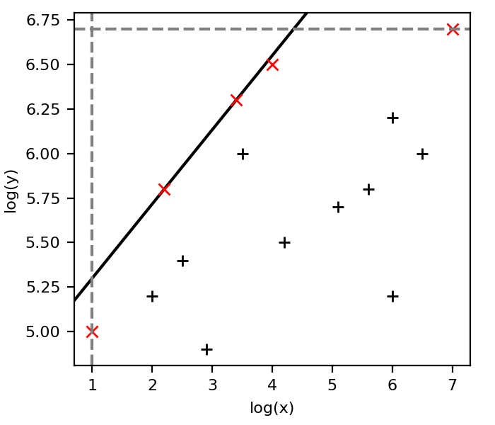
In this work the limiting functions to a number of point clouds has been computed (see Figs. 4 to 8). All of these limiting functions are computed in log-log-space ( and ) and under the assumption that the function takes the form in this space. The method will be demonstrated for the case of finding a maximum function with a positive slope to a point cloud as visible in Fig. 12 and then discuss how this algorithm can be generalized. The algorithm attempts to find a line that satisfies two conditions:
- (1)
no point is allowed left of the line,
- (2)
the area enclosed between the found line and the line marking the minimum x-value, , and maximum y-value, , (shown as dashed lines in Fig. 12) shall be maximised. Henceforth, we will call this area the ‘empty triangle’.
From the second condition we can conclude, that the line must go through at least one point of the point cloud. Otherwise we can always find a line parallel to the chosen one, that has all points to its right and produces a larger empty triangle. Therefore, we start by determining which points out of our point cloud are relevant for our calculations. These are all the points, through which we can put a line such that condition (1) is fulfilled. They are marked with red ‘x’s in Fig. 12.
A linear function through a Point can be written as:
| (21) |
Solving this equation for we can now express the area, , of the empty triangle depending on the slope :
| (22) |
It is easy to compute that for this function has one global minimum at . It is monotonic decreasing for and monotonic increasing for .
Due to condition (1) the minimum possible for a line through one of the relevant points is the one for which the line goes through its right neighbour and the maximum possible is the one for which its line goes through its left neighbour. For the relevant points with the lowest and highest only the line to one neighbour (the only one they have) has to be taken into account since all other possible lines with positive that fulfil (1) lead to a smaller empty triangle. Therefore, by comparing the areas of the empty triangles created by the connections between all the neighbouring relevant points the function fulfilling both (1) and (2) can be found. The connection producing the largest area is the solution.
Analogously a minimum function can be found by maximizing the triangle between and and the target function. For a negative slope, , and can be used to find the maximum function and and can be used to find the minimum function.