Conservation laws are key theoretical and practical tools for understanding, characterizing, and modeling nonlinear dynamical systems. However, for many complex systems, the corresponding conserved quantities are difficult to identify, making it hard to analyze their dynamics and build stable predictive models. Current approaches for discovering conservation laws often depend on detailed dynamical information or rely on black box parametric deep learning methods. We instead reformulate this task as a manifold learning problem and propose a non-parametric approach for discovering conserved quantities. We test this new approach on a variety of physical systems and demonstrate that our method is able to both identify the number of conserved quantities and extract their values. Using tools from optimal transport theory and manifold learning, our proposed method provides a direct geometric approach to identifying conservation laws that is both robust and interpretable without requiring an explicit model of the system nor accurate time information.
Discovering Conservation Laws using Optimal Transport and Manifold Learning
1 Introduction
Conservation laws are powerful constraints on the dynamics of many physical systems in nature, and the corresponding conserved quantities are essential features for characterizing the behavior of these systems. Through Noether’s theorem, conservation laws are closely tied with the symmetries of a physical system and play a key role in our understanding of physics. Conservation laws also help stabilize and enhance the performance of predictive models for complex nonlinear dynamics, e.g. symplectic integrators for Hamiltonian systems Hairer2006 and pressure projection for incompressible fluid flow GUERMOND20066011. In fact, for chaotic dynamical systems, conserved quantities are often the only features of the system state that can be reliably known far into the future. Discovering conservation laws helps us characterize the long term behavior of complex dynamical systems and understand the underlying physics.
While the conservation laws of many physical systems are well-known and often derived from known symmetries, there are still many instances where it is difficult to even determine the number of conservation laws, let alone explicitly extract the conserved quantities. As a historical example, consider the Korteweg–De Vries (KdV) equation modeling shallow water waves. The KdV equation, despite its apparent complexity, has infinitely many conserved quantities doi:10.1063/1.1664701 and is, in fact, fully solvable via an inverse scattering transform PhysRevLett.19.1095—a discovery made after significant theoretical and computational effort. Developing better general methods for identifying conserved quantities will allow us to improve our understanding of new or understudied physical systems and build more efficient and stable predictive models.
In real-world applications, an accurate model for the underlying physical system is often unavailable, forcing us to identify conservation laws using only sample trajectories of the system dynamics. One broad approach is to use modern data-driven methods based on the Koopman operator formulation of dynamical systems, which lifts the dynamics into an infinite dimensional operator space Mauroy2020. In the Koopman formalism, conserved quantities are just one type of Koopman eigenfunction with eigenvalue zero. Thus, one approach is to first apply a system identification method, such as dynamic mode decomposition schmid_2010; Williams2015ADA, sparse identification with a library of basis functions Brunton3932, or even deep learning-based approaches lusch2018deep; Champion22445; Lu2022, to model the system dynamics and then set up and solve the Koopman eigenvalue problem. Alternatively, previous work has also proposed directly setting up the eigenvalue problem by estimating time derivatives from data and then fitting the conserved quantities using a library of possible terms 8618963 or a neural network https://doi.org/10.48550/arxiv.2203.12610. These methods can work quite well but require that the measured trajectories have sufficiently low noise and high time resolution in order to accurately estimate time derivatives.
Constructing a model for a dynamical system provides much more information than just the conservation laws. In fact, even estimating time derivatives is usually not necessary if we are only interested in identifying conserved quantities. In this work, we will instead focus on an alternative approach that does not require an explicit model or detailed time information but rather takes advantage of the geometric constraints imposed by conservation laws. Specifically, the presence of conservation laws restricts each trajectory in phase space to lie solely on a lower dimensional isosurface of the conserved quantities. The dimensionality of these isosurfaces can provide information about the number of conserved quantities or constraints PhysRevLett.126.180604. Furthermore, since each isosurface corresponds to a particular set of conserved quantities, the variations in shape of the isosurfaces directly correspond to variations in the conserved quantities. In other words, we can identify and extract conserved quantities by examining the varying shapes of the isosurfaces sampled by the trajectories.
In contrast with recent work using black box deep learning methods to fit conserved quantities that are consistent with the sampled isosurfaces PhysRevResearch.2.033499; PhysRevResearch.3.L042035, we propose and demonstrate a non-parametric manifold learning approach (Fig. 1) that directly characterizes the variations in the sampled isosurfaces, producing an embedding of the space of conserved quantities. Our method first uses the Wasserstein metric from optimal transport Villani2009 to compute distances in shape space between pairs of sampled isosurfaces and then extracts a low dimensional embedding for the manifold of isosurfaces using diffusion maps 6789755; Coifman2005. Each point in this embedding corresponds to a distinct isosurface and therefore to a distinct set of conserved quantities, i.e. the embedding explicitly parameterizes the space of varying conserved quantities. Related methods have been recently suggested for characterizing molecular conformations using the 1-Wasserstein distance together with diffusion maps 9098723, performing system identification by comparing invariant measures using the 2-Wasserstein distance https://doi.org/10.48550/arxiv.2104.15138, and reconstructing normal forms using diffusion maps doi:10.1073/pnas.1620045114. Recent theoretical work has also formalized the idea of using alternative non-Euclidean norms, like the Wasserstein distance, in spectral embedding methods such as diffusion maps Kileel2021.
We provide an analytic analysis of our approach for a simple harmonic oscillator system and numerically test our method on several physical systems: the single and double pendulum, planar gravitational dynamics, the KdV equation for shallow water waves, and a nonlinear reaction–diffusion equation that generates an oscillating Turing pattern. We also demonstrate the robustness of our approach to noise in the measured trajectories, missing information in the form of a partially observed phase space, as well as approximate conservation laws (additional experiments in Appendix 10 and Appendix 8). In our comparison tests (Appendix 11), our approach outperforms prior deep learning-based direct fitting methods, all while being an order of magnitude faster. We also provide an easy-to-use codebase, which parallelizes across multiple GPUs, to make an efficient implementation of our method as accessible as possible.11 1 https://github.com/peterparity/conservation-laws-manifold-learning
2 Proposed Manifold Learning Approach
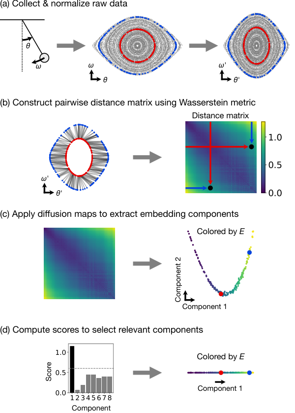
Our proposed approach uses manifold learning to identify and embed the manifold of phase space isosurfaces sampled by the trajectories of a dynamical system. In particular, we compute a diffusion map over a set of trajectories, each of which samples a particular phase space isosurface (Fig. 1a). The pairwise distances between these trajectories are given by the 2-Wasserstein distance (Fig. 1b), providing the metric structure necessary for applying diffusion maps (Fig. 1c). The manifold embedding extracted by the diffusion map corresponds directly to the space of conserved quantities (Fig. 1d). Note that this type of analysis does not require knowledge of the equations of motion (Eq. 1) and makes no direct reference to time.
2.1 Dynamical Systems
Consider a dynamical system with states that live in a -dimensional phase space and evolve in time according to a system of first order ODEs
| (1) |
with conserved quantities .
2.1.1 Conserved Quantities and Phase Space Isosurfaces
A conserved quantity is a function of the system state that does not change over time, i.e.
| (2) |
but may vary across different initial conditions. As a result, along a particular trajectory , the conserved quantities form a set of constraints
| (3) |
which depend on the values of the conserved quantities . This set of constraint equations restricts the trajectory to lie in a phase space isosurface with dimension . In fact, if any point of a trajectory lies on the isosurface , then all other points from the trajectory will lie on the same isosurface.
By studying the variations in shape of these isosurfaces, we are able to directly characterize the space of conserved quantities. In particular, consider the manifold formed by the isosurfaces in shape space.22 2 We are using the term “manifold” here rather loosely. While may be a true manifold in many cases, it is also possible for to have non-manifold structure (e.g. see our double pendulum experiment in Sec. 4.4). This manifold is parameterized by the conserved quantities . Therefore, by analyzing using manifold learning, we can extract the conservation laws of the underlying dynamical system.
2.1.2 Ergodicity and Physical Measures
To uniquely identify the isosurface associated with each trajectory, we must make several additional assumptions that will allow us to treat the set of points making up each trajectory as samples from an ergodic invariant measure on the corresponding isosurface. Specifically, we assume that, for each trajectory with conserved quantities , the dynamical system (Eq. 1) admits a physical measure medio_lines_2001 that is ergodic on the isosurface and is defined by
| (4) |
where is the Dirac measure centered on . This ensures that trajectories with the same conserved quantities will sample the same distribution on the same isosurface, allowing us to use the distribution sampled by each trajectory as a proxy for the corresponding isosurface. For more details about this assumption, see Appendix 12.4.
In practice, the sampled distribution may be lower dimensional than the corresponding isosurface if some of the conserved quantities do not vary in the dataset and instead correspond to fixed constraints, or if the dynamical system is dissipative. In the former case, this does not affect our ability to uniquely identify a distribution with an isosurface and its corresponding set of conserved quantities, meaning that we are able to apply this approach even if the provided phase space is much larger than the intrinsic phase space of the dynamical system. In the latter case, the dissipative nature of the system may cause information about conservation laws relevant during the transient portion of the dynamics to be lost, but we are still able to use our approach to identify conserved quantities relevant for the long term behavior of the system.
2.2 Wasserstein Metric
To analyze the isosurface shape space manifold —i.e. the manifold of conserved quantities—using manifold learning methods, we need to place some structure on the points . Having associated each isosurface with a corresponding distribution defined by an ergodic physical measure , we choose to lift the Euclidean metric on the phase space into the space of distributions using the 2-Wasserstein metric from optimal transport
| (5) |
where the cost function is the squared Euclidean distance, and is a valid transport map between and Villani2009.
For discrete samples, the 2-Wasserstein distance between two sets of sample points and is defined as
| (6) |
where the cost matrix , and the transport matrix is subject to the constraints
| (7) | ||||
To efficiently compute an entropy regularized form of this optimization problem, we use the Sinkhorn algorithm NIPS2013_af21d0c9 and estimate the Wasserstein distance as a debiased Sinkhorn divergence pmlr-v119-janati20a.
One important subtlety in this construction is the choice of the ground metric for optimal transport. As previously mentioned, we use a Euclidean metric on the phase space, which implicitly imposes a choice of units to make the phase space dimensionless. In fact, there is no canonical choice for the ground metric, and different choices result in different Wasserstein metrics on the shape space. While, in theory, information about all conserved quantities will be embedded in the resulting distance matrix regardless of the choice of metric, the metric ultimately determines how easy it is to access this information. For example, when multiple conserved quantities are present, the relative effect of each conserved quantity on the computed Wasserstein distances will determine how prominent each conserved quantity is and how easily it is identified using manifold learning. To partially mitigate this issue and improve consistency, we normalize each component of our data to have a maximum absolute value of 1 before computing the pairwise Wasserstein distances.
2.3 Diffusion Maps
Using the structure provided by the Wasserstein metric, we then use diffusion maps to generate an embedding for . The diffusion map manifold learning method uses a spectral embedding algorithm applied to an affinity matrix to construct a low dimensional embedding of the data manifold 6789755; Coifman2005. Using the pairwise Wasserstein distances computed from discrete samples provided by the trajectory data (Eq. 6), we first construct a kernel matrix using a Gaussian kernel
| (8) |
and then scale it to form an affinity matrix for our spectral embedding
| (9) |
where , and is a hyperparameter. The spectral embedding algorithm then takes this affinity matrix and constructs a normalized graph Laplacian
| (10) |
where is the identity matrix. The eigenvectors corresponding to the smallest eigenvalues (excluding ) of the Laplacian then provide an approximate low dimensional embedding of the manifold of conserved quantities . In our experiments, we set so that the Laplacian computed by the spectral embedding algorithm approximates the Laplace–Beltrami operator 6789755.
To estimate the dimensionality of and to choose which eigenvectors to include in our embedding, we use a heuristic score that combines a measure of relevance, given by a length scale computed from the Laplacian eigenvalues, with a previously suggested measure of “unpredictability” for minimizing redundancy pfau2018minimally (alternative approaches also exist DSILVA2018759; vonLindheim2018). To construct our embedding, we only include the Laplacian eigenvectors with score above a chosen cutoff value and discard the rest as either noise or redundant embedding components. To determine the cutoff, we perform a sweep of the cutoff value looking for robust ranges and find that a cutoff of 0.6 works well across all of our experiments, which consist of a wide variety of datasets and dynamical systems. See Appendix 6 for more details.
3 Analytic Result for the Simple Harmonic Oscillator
In the case of a simple harmonic oscillator (SHO) without measurement noise and in the infinite sample limit, we are able to explicitly derive an analytic result for our proposed procedure. We first compute the pairwise distances provided by the Wasserstein metric and then derive the embedding produced by a diffusion map, which corresponds to the conserved energy of the SHO.
3.1 Wasserstein Metric: Constructing the Isosurface Shape Space
Consider a SHO with Hamiltonian
| (11) |
given in terms of position and momentum . The SHO energy isosurfaces form concentric ellipses in a 2D phase space. Choosing units such that and , we obtain concentric circles with uniformly distributed samples (assuming a uniform sampling in time). The 2-Wasserstein distance between a pair of uniformly distributed circular isosurfaces is simply given by the difference in radii . This is because, due to the rotational symmetry of the two distributions, the optimal transport plan for an isotropic cost function is to simply move each point on isosurface 1 radially outward (or inward) to the point on isosurface 2 with the same angle .
This result does not meaningfully change with a different choice of units, which is equivalent to rescaling the phase space coordinates . If we rescale by factors , our cost function simply becomes
| (12) | ||||
where we label points on the isosurfaces by their angle on the original circular isosurfaces. The SHO optimal transport plan takes on isosurface 1 to the point with the same angle on isosurface 2, and for the SHO is invariant to coordinate rescaling (Appendix 14). Therefore, the total transport cost is
| (13) |
so the 2-Wasserstein distance is
| (14) |
i.e. the same result modulo a constant factor. While this is not a general result, we find that our approach is often fairly robust to such changes, including the extreme case of scaling some phase space coordinates all the way down to zero resulting in a partially observed phase space (Appendix 10).
3.2 Diffusion Maps: Extracting the Conserved Energy
Once we have pairwise distances in the isosurface shape space, we can use diffusion maps to study the resulting manifold of isosurface shapes. With sufficient samples, the operator constructed by the diffusion map should converge to the Laplace–Beltrami operator on the manifold. For the SHO, the isosurface shape space is isomorphic to with each circular isosurface mapped to its radius. If we sample trajectories with radii for some maximum energy , then the manifold is a real line segment, and the resulting Laplacian operator (with open boundary conditions) has eigenvalues and corresponding eigenvectors . Therefore, the first eigenvector or embedding component
| (15) |
successfully encodes the conserved energy and is, in fact, a monotonic function of the energy.
4 Numerical Experiments
To demonstrate and empirically test our method for discovering conservation laws, we generate datasets from a wide range of dynamical systems, each consisting of randomly sampled trajectories with different initial conditions and the corresponding conserved quantities. Note that we use the dimensionless form of each dynamical system. All of the code necessary for reproducing our results is available at https://github.com/peterparity/conservation-laws-manifold-learning.
4.1 Simple Harmonic Oscillator
We first numerically test our analytic result for the SHO and obtain good agreement (Fig. 2) using both the default scaling (Figs. 2a–d) as well as the position only scaling , (Figs. 2e–h), which effectively reduces the dimension of the phase space. A linear fit of the first embedding component from the diffusion map with the analytically predicted component (Eq. 15) achieves a correlation coefficient of for the default scaling and for the position only scaling. We also verify that the heuristic score (Appendix 6) accurately determines that there is only one relevant embedding component (Figs. 2c,g), which corresponds to the conserved energy.
4.2 Simple Pendulum
To demonstrate our method on a simple nonlinear dynamical system, we analyze a simple pendulum that has a 2D phase space consisting of the angle and angular momentum (Fig. 3a). The equations of motion are
| (16) | ||||
This system has a single scalar conserved quantity
| (17) |
corresponding to the total energy of the pendulum, so the trajectories form 1D orbits in phase space (Fig. 3b).
Our method is able to correctly determine that there is only a single conserved quantity (Fig. 3c) corresponding to the energy of the pendulum (Fig. 3d). The single extracted embedding component is monotonically related to the energy with Spearman’s rank correlation coefficient . We are also able to achieve similar results () with a high level of Gaussian noise (standard deviation ) added to the raw trajectory data (Figs. 3e–h), showing that our approach is quite robust to measurement noise.
4.3 Planar Gravitational Dynamics

To test our method on a system with multiple conserved quantities, we simulate the gravitational system of a planet orbiting a star with much greater mass (Fig. 4a). We fix the orbits to all lie in a 2D plane, giving us an effectively 4D phase space. The resulting equations of motion are
| (18) | ||||
This system has one scalar and two vector conserved quantities
| (19) | ||||
which, in our 4D phase space, reduces to three scalar conserved quantities: the total energy (or equivalently, the semi-major axis ), the angular momentum , and the orbital orientation angle , which is the angle of the LRL vector relative to the -axis. As a result, the trajectories also form 1D orbits in the phase space (Fig. 4b).
Our approach accurately identifies the three conserved quantities (Fig. 4c), and the extracted embedding corresponds most directly to the geometric features of the orbits (Figs. 4d–f). The first two components embed the semi-major axis vector with magnitude given by the semi-major axis , which is related to the energy , and orientation given by the orientation angle of the elliptical orbit (Figs. 4d,e). The third relevant component (component 6) embeds the angular momentum (Fig. 4f). See Appendix 6.1 for details on choosing a cutoff to identify the relevant components. A linear fit of the identified relevant embedding components with () has () and rank correlation (). A similar linear fit with has and .
This example demonstrates that, for a system with multiple conserved quantities, the ground metric for optimal transport controls the relative scale of each conserved quantity in the extracted embedding. In this case, the geometry of the shape space is dominated by changes in the semi-major axis and orientation angle , whereas changes in the angular momentum , which controls the eccentricity of the orbit, play a more minor role and thus appear in a later embedding component with a lower score (Fig. 4c).
4.4 Double Pendulum

To test our approach on a non-integrable system with higher dimensional isosurfaces, we study the classic double pendulum system (Fig. 5a) with unit masses and unit length pendulum arms. This system has a 4D phase space, consisting of the angles and the angular velocities of the two pendulums (Fig. 5b), and only has a single scalar conserved quantity
| (20) |
corresponding to the total energy. However, the double pendulum system has both chaotic and non-chaotic phases. In particular, at high energies, the system is chaotic and only conserves the total energy, while at low energies, the system behaves more like two coupled harmonic oscillators with two independent (approximately) conserved energies
| (21) | ||||
corresponding to the two modes of the coupled oscillator system. Therefore, we expect to see two distinct phases in our extracted embedding: one with a single conserved quantity at high energy and another with two approximately conserved quantities at low energy, which approximately sum to .
At first glance, it appears as though our method has only identified a single relevant component corresponding to the conserved total energy (Figs. 5c,e) with rank correlation . However, if we restrict ourselves to low energy trajectories with first embedding component , we find that there is a region of the shape space that is two-dimensional, corresponding to the two independently conserved energies of the low energy non-chaotic phase where the double pendulum behaves like a coupled oscillator system with two distinct modes. For the low energy trajectories, a linear fit of the now two relevant components with () has rank correlation (). If we restrict ourselves to even lower energy trajectories with , a similar linear fit for () has rank correlation ().
This analysis of the double pendulum shows that our method can still provide significant insight into complex dynamical systems with multiple phases involving varying numbers of conserved quantities. This manifests itself as manifolds of different dimensions in shape space that are stitched together at phase transitions, presenting a significant challenge for most manifold learning methods. In this example, this difficulty is reflected in the performance of the heuristic score (Fig. 5c,d), which has trouble telling whether the embedding is one or two dimensional precisely because it is a combination of both a one and two dimensional manifold. The embedding, on the other hand, remains very informative despite the sudden change in dimensionality and allows us to identify interesting features of the system, such as nonlinear periodic orbits (see Appendix 9). The effectiveness of diffusion maps when handling these complex situations has been previously observed in parameter reduction applications HOLIDAY2019419 and is worth studying in more detail in the future.
4.5 Oscillating Turing Patterns
Next, we consider an oscillating Turing pattern system that is both dissipative and has a much higher dimensional phase space than our previous examples. In particular, we study the Barrio–Varea–Aragón–Maini (BVAM) model BARRIO1999483; PhysRevE.86.026201
| (22) | ||||
with , , and , following Aragón et al. PhysRevE.86.026201 who showed that this set of parameters results in a spatial Turing pattern that also exhibits chaotic oscillating temporal dynamics, on a periodic domain with size . The phase space of the BVAM system consists of two functions and 33 3 In our method, each trajectory is treated as an unordered set of sample points in phase space, so we refer to the phase space as in a slight abuse of notation. which we discretize on a mesh of size , giving us an effective phase space dimension of . Because this system is dissipative, we will focus on characterizing the long term behavior of the dynamics, i.e. the oscillating Turing pattern, which appears to have a conserved spatial phase for our chosen set of parameters corresponding to the spatial position of the Turing pattern. In the language of dynamical systems, parameterizes a continuous set of attractors for this dissipative system.
Our method successfully identifies the spatial phase but embeds the angle as a circle in a 2D embedding space (Fig. 6)—a result of the periodic topology of . While this shows that the number of relevant components determined by our heuristic score may not always match the true manifold dimensionality, such cases are often easily identified by examining the components directly (Fig. 6c) or by cross checking with an intrinsic dimensionality estimator https://doi.org/10.48550/arxiv.2106.04018. A linear fit of the two relevant components with () has () and (). This example both tests our method on a high dimensional phase space and demonstrates how our approach can be applied to dissipative systems to study long term behavior.

4.6 Korteweg–De Vries Equation

For many spatiotemporal dynamical systems, the conservation laws are local in nature. Locality can significantly simplify the analysis of the conserved quantities and suggests a way to restrict the type of conserved quantities identified by our method. Specifically, we can adapt our approach to focus on local conserved quantities by replacing the raw states (Fig. 7a) by a distribution of local features (Fig. 7b), removing the explicit spatial label and providing a fully translation invariant representation of the state. Then, instead of using the Euclidean metric in the original phase space, we use the energy distance https://doi.org/10.1002/wics.1375; pmlr-v89-feydy19a between the distributions of local features as the ground metric for optimal transport.
To demonstrate this method for identifying local conserved quantities, we consider the Korteweg–De Vries (KdV) equation
| (23) |
The KdV equation is fully integrable PhysRevLett.19.1095 and has infinitely many conserved quantities doi:10.1063/1.1664701, the most robust of which are the most local conserved quantities expressible in terms of low order spatial derivatives. To focus on these robust local conserved quantities, we use finite differences (i.e. ) as our local features, allowing us to restrict the spatial derivative order of the identified conserved quantities. In this experiment, we only take and , meaning that the identified local conserved quantities will only contain up to first order spatial derivatives. For the KdV equation, there are three such local conserved quantities:
| (24) | ||||
where and are often identified as “momentum” and “energy”, respectively doi:10.1063/1.1664701. These local conserved quantities also have direct analogues in generalized KdV-type equations, hinting at their robustness 1937-1632_2018_4_607.
Our method successfully identifies three relevant components (Fig. 7c) corresponding to (d–f) the three local conserved quantities (Eq. 24). Linear fits of these components to , , and have rank correlations , , and , respectively. This result shows how our approach can be adapted to incorporate known structure, such as locality and translation symmetry, in applications to complex high dimensional dynamical systems.
5 Discussion
We have proposed a non-parametric manifold learning method for discovering conservation laws, tested our method on a wide variety of dynamical systems—including complex chaotic systems with multiple phases and high dimensional spatiotemporal dynamics—and also shown how to adapt our approach to incorporate additional structure such as locality and translation symmetry. While our experiments use dynamical systems with known conserved quantities in order to validate our approach, our method does not require any a priori information about the conserved quantities. Our method also does not assume or construct an explicit model for the system nor require accurate time information like previous approaches 8618963; https://doi.org/10.48550/arxiv.2203.12610, only relying on the ergodicity of the dynamics modulo the conservation laws (Sec. 2.1.2). As a result, our approach is also quite robust to measurement noise and can often deal with missing information such as a partially observed phase space (Figs. 2e–h, Figs. 3e–h, Appendix 10).
Compared with recently proposed deep learning-based methods PhysRevResearch.2.033499; PhysRevResearch.3.L042035, our approach is substantially more interpretable since it relies on explicit geometric constructions and well-studied manifold learning methods that directly determine the geometry of the shape space and, therefore, the identified conserved quantities. This is reflected in our ability to explicitly derive the expected result for the simple harmonic oscillator (Sec. 3), as well as in the identified conserved quantities in many of our experiments. For example, the embedding of the semi-major axis vector in the planar gravitational dynamics experiment (Sec. 4.3) stems directly from the elliptical geometry of the orbits and their orientation in phase space, which is captured by the Euclidean ground metric and lifted into shape space by optimal transport. Our method also correctly captures the subtleties of the double pendulum system (Sec. 4.4) by providing an embedding that shows both a 1D manifold at high energies and a 2D manifold at low energies—a difficult prospect for deep learning approaches that try to explicitly fit conserved quantities. In addition, we empirically find that our method outperforms existing direct fitting approaches PhysRevResearch.2.033499; PhysRevResearch.3.L042035. See Appendix 11 for a comparison benchmark using our planar gravitational dynamics dataset.
Our manifold learning approach to identifying conserved quantities provides a new way to analyze data from complex dynamical systems and uncover useful conservation laws that will ultimately improve our understanding of these systems as well as aid in developing predictive models that accurately capture long term behavior. While our method does not provide explicit symbolic expressions for the conserved quantities (which may not exist in many cases), we do obtain a full set of independent conserved quantities, meaning that any other conserved quantity will be a function of the discovered ones. Our method also serves as a strong non-parametric baseline for future methods that aim to discover conservation laws from data. Finally, we believe that similar combinations of optimal transport and manifold learning have the potential to be applied to a wide variety of other problems that also rely on geometrically characterizing families of distributions, and we hope to investigate such applications in the near future.
Acknowledgments
We would like to acknowledge useful discussions with Justin Solomon, Ziming Liu, Andrew Ma, Samuel Kim, Charlotte Loh, and Ruba Houssami. P.Y.L. gratefully acknowledges the support of the Eric and Wendy Schmidt AI in Science Postdoctoral Fellowship, a Schmidt Futures program. This research is supported in part by the U.S. Department of Defense through the National Defense Science & Engineering Graduate Fellowship Program; the National Science Foundation under Cooperative Agreement PHY-2019786 (The NSF AI Institute for Artificial Intelligence and Fundamental Interactions, http://iaifi.org/); the U.S. Army Research Office through the Institute for Soldier Nanotechnologies at MIT under Collaborative Agreement Number W911NF-18-2-0048; the Air Force Office of Scientific Research under the award number FA9550-21-1-0317; and the United States Air Force Research Laboratory and the United States Air Force Artificial Intelligence Accelerator under Cooperative Agreement Number FA8750-19-2-1000. The views and conclusions contained in this document are those of the authors and should not be interpreted as representing the official policies, either expressed or implied, of the United States Air Force or the U.S. Government. The U.S. Government is authorized to reproduce and distribute reprints for Government purposes notwithstanding any copyright notation herein.
Declarations
Competing interests
The authors declare no competing interests.
Data availability
All the datasets used in this study can be generated using the publicly available data generation scripts provided at https://github.com/peterparity/conservation-laws-manifold-learning.
Code availability
All the code necessary for reproducing our results is publicly available at https://github.com/peterparity/conservation-laws-manifold-learning.
Author contributions
All three authors contributed to the conception, design, and development of the proposed method. P.Y.L. implemented, tested, and refined the method and also generated the datasets. The manuscript was written by P.Y.L. with support from R.D. and M.S.
6 Heuristic Score for a Minimal Diffusion Maps Embedding
Traditionally, diffusion maps Coifman2005 and Laplacian eigenmaps 6789755 leave the embedding dimension as a hyperparameter and simply use the eigenvectors corresponding to the smallest eigenvalues to construct the embedding. In practice, the embedding dimension is often chosen for convenience (e.g. in visualization applications) or by examining the eigenvalues and looking for a sharp increase in the magnitude of the eigenvalues that would separate the signal from the noise. Because identifying the number of conservation laws is an important step in our approach, we refine this heuristic by directly computing an approximate length scale
| (25) |
where is the scale factor from the Gaussian kernel (Eq. 8) used to construct the Laplacian matrix . We derive this length scale by considering the normalized kernel to be an approximation of the heat kernel , implying that the length scales associated with the Laplace–Beltrami operator are given by
| (26) |
We then divide by to obtain the relative length scale
| (27) |
which can be used as a heuristic measure of relevance—components with a small relative length scale are more likely to be noise. Compared with directly using the eigenvalues , we find this heuristic to be less sensitive to the choice of in the kernel.

In addition to noise, there is the common problem of redundant embedding components that stem from the structure of the Laplacian operator: higher order modes of previous eigenvectors often appear before more informative eigenvectors corresponding to new manifold directions. This problem is clearly illustrated in the planar gravitational dynamics experiment (Sec. 4.3), where components 3, 4, and 5 are all redundant with components 1 and 2 but component 6 is a new and relevant conserved quantity (Figs. 8d–f). To address this issue, the key observation is that, while all components of the diffusion map are linearly independent, redundant components are still predictable (via a nonlinear function) from previous components. Therefore, we require a measure of “unpredictability” that allows us to identify redundancies. We choose the heuristic proposed by Pfau and Burgess pfau2018minimally that uses a nearest neighbor estimator (using 5 nearest neighbors) to determine whether a new embedding component is too predictable and therefore redundant. Alternative methods for dealing with these redundant components, also called repeated eigendirections or higher harmonics, have been proposed that use local linear regression to detect redundant components DSILVA2018759 or adapt the diffusion kernel to be anisotropic for chosen components vonLindheim2018.
Our final heuristic score (Fig. 8c)
| (28) |
is the product of the relative length scale (Fig. 8a) and the unpredictability measure (Fig. 8b). We find this simple combined score performs well for identifying relevant embedding components by removing both noise components as well as redundant components.
6.1 Choosing a Score Cutoff
To use the heuristic score to identify the number of conserved quantities and construct a minimal embedding, we require a score cutoff to separate relevant components that we keep in our embedding from irrelevant components that we discard. To choose this cutoff, we sweep cutoff values in the interval , compute the embedding size (i.e. the number of relevant components) based on the chosen cutoff, and then examine the result to identify a robust value for the cutoff (Fig. 9). Specifically, we look for wide plateaus in the embedding size that indicate robustness to the value of the cutoff and find that a cutoff of 0.6 works well in all of our experiments. In practice, we would treat a cutoff of 0.6 as a good starting point but recommend analyzing a range of cutoff values to find a robust choice of cutoff, as illustrated in Fig. 9.
7 Additional Method Details
All of the code necessary for generating our datasets, applying our method, and reproducing our results is available at https://github.com/peterparity/conservation-laws-manifold-learning.
7.1 Sinkhorn Algorithm
7.1.1 Entropy Regularized Optimal Transport
We compute an approximate 2-Wasserstein distance using the Sinkhorn algorithm NIPS2013_af21d0c9, which solves an entropy regularized relaxation of the optimal transport problem
| (29) |
where the cost matrix and the entropy . reduces to the exact 2-Wasserstein distance (Eq. 6) as . For , the entropy regularization introduces a smoothing bias that manifests as a nonzero “self-distance” . This can be corrected by instead using the Sinkhorn divergence pmlr-v89-feydy19a; pmlr-v119-janati20a
| (30) | ||||
as our estimate for the 2-Wasserstein distance, which explicitly subtracts off this self-distance. In our experiments, we use a convergence threshold of and a decaying entropy regularization parameter that starts at and decays by a factor of at each step until it reaches a target of .
Note that the Sinkhorn algorithm is a general approach for solving entropy-regularized optimal transport and is equally good at approximating a 1-Wasserstein distance (or Earth mover’s distance). We experimented with using 1-Wasserstein vs. 2-Wasserstein distances and did not find a significant difference in the performance of our method.
7.1.2 Time Complexity
With samples per trajectory, the Sinkhorn algorithm solves the entropy regularized optimal transport problem in time for an -accurate solution NIPS2017_491442df; pmlr-v80-dvurechensky18a using space (without explicit storing the cost matrix https://doi.org/10.48550/arxiv.2201.12324). Therefore, the time complexity of computing approximate Wasserstein distances for all pairs of trajectories is for a dataset containing total trajectories. This computation is currently the performance bottleneck of our approach (Appendix 12.1) but is easily parallelized over multiple GPUs using the OTT-JAX library https://doi.org/10.48550/arxiv.2201.12324.
7.2 Diffusion Maps
7.2.1 Choice of Manifold Learning Method

Unlike many standard manifold learning applications, our input to the manifold learning method is not a set of points in Euclidean space but rather a pairwise Wasserstein distance matrix. Many popular methods, such as local linear embedding doi:10.1126/science.290.5500.2323 and local tangent space alignment doi:10.1137/S1064827502419154, explicitly require the data to be embedded in a Euclidean space and so are not applicable for our problem. In addition to diffusion maps, we also experimented with Isomap doi:10.1126/science.290.5500.2319, which can also take a distance matrix as input. However, we found Isomap embeddings to be noisier and less reliable than diffusion map embeddings (e.g. see Fig. 10). Diffusion maps Coifman2005 or Laplacian eigenmaps 6789755 also provide an effective way to estimate manifold dimensionality and choose relevant embedding components (Appendix 6).
7.2.2 Gaussian Kernel Width
The primary hyperparameter in our diffusion maps algorithm is the width parameter of the Gaussian kernel (Eq. 8). Generally speaking, we should choose to be large enough to avoid noise induced by sparse sampling but small enough for the true heat kernel to be well approximated by the Gaussian kernel 6789755. We choose such that the corresponding standard deviation of the Gaussian kernel is equal to the maximum distance to the th nearest neighbor.
In practice, especially when the relevant embedding components are well separated from the noise in terms of length scale (Eq. 25), we find the diffusion map to be fairly insensitive to the choice of , which we generally set to nearest neighbors. The only exception is for the planar gravitational dynamics dataset, where we use . This is because the angular momentum—the least prominent of the three conserved quantities—has a slightly poorer reconstruction for () and gets pushed back to component 10 of the embedding. While it is still clearly identifiable from noise, it requires a lower heuristic score cutoff of around and is easier to miss.
7.2.3 Noise Robustness
To improve the noise robustness of our diffusion map, we follow Karoui and Wu 10.1214/14-AOS1275 and replace the diagonal of the affinity matrix (Eq. 9) with zeros, i.e.
| (31) |
before constructing the Laplacian matrix . Because this induces an overall shift in the eigenvalues of the Laplacian that interacts poorly with our length scale heuristic (Eq. 25), we correct for this by subtracting off the normalized mean shift
| (32) |
from the Laplacian matrix to obtain the corrected Laplacian
| (33) |
which we use to generate our embeddings.
7.2.4 Time Complexity
For a fixed number of embedding dimensions and a dense kernel matrix with entries ( being the number of trajectories), diffusion maps have time complexity and space complexity . In our experiments, computing the diffusion map is very fast with run times under one second for every dataset we tested.
7.2.5 Out-of-Sample Embedding
One complication of manifold learning methods like diffusion maps is that they do not provide an explicit way to embed new out-of-sample data. A naive approach would be to rerun the diffusion map algorithm on a combined dataset consisting of the original data used to create the embedding and the new data. However, this does not retain the original embedding and, in some cases, may be computationally prohibitive. A popular approach that does retain the original embedding is the Nyström method NIPS2003_cf059682, which embeds a new point using its pairwise distances with the original data and scales as . For even faster embedding, landmark diffusion maps offer a significant speed-up by choosing a small subset of landmark points to use during Nyström out-of-sample embedding LONG2019190. This also has the added benefit of a reduced memory footprint, since only the landmark points need to be retained for embedding.
8 Langevin Harmonic Oscillator

To demonstrate our method on a simple example of a dynamical system with approximately conserved quantities at short time scales but no true conserved quantities, we consider an under-damped harmonic oscillator that is weakly coupled to a heat bath. The resulting dynamics are governed by the Langevin equations
| (34) | ||||
where the damping . is a Gaussian random process (i.e. Brownian motion) with zero mean and . We set the temperature of the heat bath to be . At short times and , the energy is approximately conserved. At long times , all trajectories will sample a stationary distribution with variance and no conserved quantities.
We generate four datasets for this system, each with 200 trajectories and 200 samples over different periods of time, i.e. with sampling time . This allows us to study how changing the sampling time —the time scale over which we identify approximately conserved quantities—changes the embedding produced by our approach. Over short time scales, the time-averaged energy is still a distinguishing feature of the trajectories and acts as an approximately conserved quantity (Figs. 11a–d). Over longer time scales, the energy becomes less and less relevant until, finally, the system reaches a stationary distribution (Figs. 11e–h).
8.1 Separation of Time Scales and Dependence on and
As previously noted, the energy of the Langevin harmonic oscillator is only conserved over time scales much less than the time scales associated with dissipation and random forcing . However, this approximate conservation law is only meaningful if the energy is roughly conserved over a time scale much greater than the period of oscillation, which is of order one in our units. In other words, approximate conservation laws only appear when there is a separation of time scales between fast conservative dynamics (e.g. the oscillations of our harmonic oscillator) and slow non-conservative dynamics (e.g. dissipation and forcing).
Thus, for and , we expect to have an approximately conserved energy at intermediate time scales and . As , there is no longer an intermediate time scale for which the approximate conservation law holds. This is precisely what we see when we apply our method for identifying conservation laws to Langevin harmonic oscillators with varying and using sampling times (Fig. 12).
The rank correlation (Fig. 12a) shows the alignment of the first embedding component with the time-averaged energy , while the prominence (Fig. 12b) of the heuristic score shows how well distinguished the first component is from the remaining noisy components. We find that for small and , our approach successfully identifies the approximately conserved energy at intermediate time scales or (as shown by the high rank correlation and high score prominence). For longer time scales or larger and , the approximate conservation law no longer holds and so our method identifies no conserved quantities (as shown by the low score prominence).
9 Nonlinear Periodic Orbit of the Double Pendulum
In addition to the chaotic and linear non-chaotic phases, the double pendulum can also exhibit other kinds of complex behavior, including highly nonlinear periodic orbits. In our extracted embedding (Fig. 13a), we see an example of such a nonlinear periodic orbit (Figs. 13b,c). The placement of this periodic orbit in the embedding also meaningfully connects it with the low energy in-phase mode from the linear coupled oscillator regime (Fig. 5g), i.e. this periodic orbit can be thought of as a nonlinear high energy extension of the low energy in-phase mode.
10 Robustness to Noise & Partial Observations
| \topruleDataset | Conserved Quantity | |
| \midruleSimple Pendulum: Position Only | 0.998 | |
| Simple Pendulum: Position Only + Noise | 0.996 | |
| Planar Gravitational Dynamics:
Position Only |
0.994 | |
| 0.993 | ||
| 0.968 | ||
| Planar Gravitational Dynamics:
Noise |
0.994 | |
| 0.992 | ||
| 0.945 | ||
| Double Pendulum:
Position Only |
0.996 | |
| 0.931∗ | ||
| 0.945∗ | ||
| \bottomrule |

To further demonstrate the robustness of our approach, we show several additional experiments on the simple pendulum, planar gravitational dynamics, and double pendulum datasets. For the simple pendulum, our method still performs well when using only angle measurements, i.e. a partially observed phase space (Fig. 14a). In fact, even if we add Gaussian noise (standard deviation ) to the raw trajectory data in addition to using a partially observed phase space, we still obtain a similar result (Fig. 14b). Similarly, for planar gravitational dynamics with only position data or with added Gaussian noise (), our method is still able to identify the three conserved quantities (Figs. 14c,d). For the double pendulum, we again see that we retain the same detail in the extracted embedding using only position data (Fig. 15). The corresponding rank correlations with the ground truth conserved quantities are given in Table 1.
The robustness of our method to both noise and partial observations is largely a consequence of using the Wasserstein distance as our metric for comparing trajectories. In our problem formulation, we consider the isosurfaces with constant conserved quantities and ask for a metric for measuring distances between isosurfaces. Because the Wasserstein distance measures distances between distributions rather than disjoint isosurfaces, it can easily generalize to noisy or partially observed data where the trajectories are no longer strictly disjoint. An alternative choice of metric, e.g. the Hausdorff distance between sets in a metric space 10.1007/978-3-030-04747-4_10, does not have this nice property and would be much more susceptible to noise or partial observations. On the other hand, because the Wasserstein distance distinguishes between different distributions, it is susceptible to other forms of corruption such as sampling inhomogeneity (discussed in Appendix 12.3). In most cases, we believe that this tradeoff is worth it to retain the high degree of robustness as long as one is aware of the limitations.
11 Comparison with Direct Fitting Methods
| \topruleDataset | Method | Conserved Quantity | |
|---|---|---|---|
| \midruleClean,
Fully Observed |
Manifold Learning (Ours) | 0.994 | |
| 0.992 | |||
| 0.970 | |||
| ConservNet | 0.882 | ||
| 0.029 | |||
| 0.002 | |||
| SNN | 0.948 | ||
| 0.024 | |||
| 0.007 | |||
| \midruleNoisy (), Fully Observed | Manifold Learning (Ours) | 0.994 | |
| 0.992 | |||
| 0.945 | |||
| ConservNet | 0.178 | ||
| 0.003 | |||
| 0.069 | |||
| SNN | 0.031 | ||
| 0.005 | |||
| 0.025 | |||
| \midruleClean, Partially Observed (Position Only) | Manifold Learning (Ours) | 0.994 | |
| 0.993 | |||
| 0.968 | |||
| ConservNet | 0.892 | ||
| 0.036 | |||
| 0.015 | |||
| SNN | 0.916 | ||
| 0.010 | |||
| 0.060 | |||
| \bottomrule |
Only a few alternative approaches PhysRevLett.126.180604; PhysRevResearch.2.033499; PhysRevResearch.3.L042035 have been proposed for identifying conservation laws from trajectory samples without time information (e.g. any methods that require time derivative estimates of the system state are not applicable). These alternatives all fall into a broad category that we term “direct fitting” methods, which attempt to directly fit a parameterized function of the system state to be constant over each trajectory. This can be accomplished using a variety of methods and optimization objectives but all generally require that the system state is fully observed and that the observed trajectories have low noise. These restrictions ensure that the basic assumption of direct fitting methods—that there exists a well-defined function from the observed state to the conserved quantities—is fulfilled.
AI Poincaré PhysRevLett.126.180604 uses a symbolic regression approach to directly obtain an interpretable expression for the conserved quantities in terms of a library of symbolic expressions. While this method can sometimes give the exact expected conservation laws, AI Poincaré relies heavily on the applicability of symbolic regression, and, in cases where there is no simple symbolic expression, it will often fail. For example, for the planar gravitational dynamics dataset (named the “Kepler problem” in PhysRevLett.126.180604), AI Poincaré fails to identify the conserved quantity associated to the orientation angle of the orbit due to its somewhat awkward symbolic representation PhysRevLett.126.180604.
The two remaining direct fitting methods, Siamese Neural Network (SNN) PhysRevResearch.2.033499 and ConservNet PhysRevResearch.3.L042035, both use a neural network as the parameterized function to fit the trajectory data. One important limitation of both of these approaches is their inability to discover more than a single conserved quantity per dataset. In both works PhysRevResearch.2.033499; PhysRevResearch.3.L042035, identifying a second conserved quantity requires generating a new dataset while holding the first discovered conserved quantity fixed. Generating such a dataset as part of the method pipeline assumes both access to and fine-grained control of the data generating process, which is often not available in practice. We benchmark our manifold learning approach against these two methods on the planar gravitational dynamics dataset, variations of which (under the name “Motion in a central potential” and “Kepler problem”) were also previously studied in both works PhysRevResearch.2.033499; PhysRevResearch.3.L042035. Because we only use a single dataset, we only expect these direct fitting methods to identify a single conserved quantity. We also compare these methods on the noisy and partially observed versions of the dataset to understand their limitations.
Implementations for both direct fitting methods were adapted from code released by PhysRevResearch.3.L042035 since reference code for PhysRevResearch.2.033499 is unavailable. Following PhysRevResearch.3.L042035, our benchmark uses a simple fully connected neural network with four hidden layers of size 320, Mish activations https://doi.org/10.48550/arxiv.1908.08681, and an Adam optimizer kingma2015adam with learning rate . We use a batch size of 1000 for the SNN and 200 (fixed by the number of samples per trajectory) for ConservNet. We train each network for 1000 epochs44 4 We did not see any improvement on our dataset when the networks were trained for 50,000 epochs, as recommended by PhysRevResearch.3.L042035. and then compute the rank correlation of the fitted function with the ground truth conserved quantities (Table 2).
The results show that, as expected, the direct fitting methods only learned a single conserved quantity for the dataset (Table 2). Even for the single conserved quantity identified by SNN and ConservNet, we see that our manifold learning method outperforms both direct fitting methods in all settings while also identifying all three conserved quantities. Training for SNN and ConservNet took between 40–50 minutes for 1000 epochs on a single RTX 2080 Ti GPU and does not appear to benefit significantly from using larger batch sizes and additional compute resources. In comparison, our method—which is limited primarily by the Wasserstein distance estimation (Appendix 12.1)—takes around 40 seconds to run on eight RTX 2080 Ti GPUs and 5–6 minutes on a single RTX 2080 Ti GPU.
12 Additional Discussion & Limitations
12.1 Time & Space Complexity
For a dataset with trajectories and with samples per trajectory, our approach is currently limited by the computational cost of estimating the 2-Wasserstein distance for all pairs of trajectories (Table 3), giving a time complexity of (Appendix 7.1). To scale to much larger datasets, we have several choices to improve the run time performance.
One simple adjustment to speed up the convergence of the Sinkhorn algorithm is to allow for a significantly larger target regularization parameter . The result, in fact, interpolates between the Wasserstein metric () and a maximum mean discrepancy (MMD) metric () pmlr-v89-feydy19a. However, to improve the time complexity of our approach as we scale to large , we may have to consider more approximate approaches. A popular option is to first subsample the data to form minibatches of size , solve the much smaller optimal transport problem, and then average the resulting estimates for the Wasserstein distance pmlr-v84-genevay18a; pmlr-v108-fatras20a. For a fixed number of epochs of averaging, this approach would give us linear scaling with the number of samples .
To improve the scaling with the number of trajectories , we may be able to take advantage of the sparse structure of the kernel matrix when the total number of conserved quantities . That is, when the dimension of the embedded manifold (corresponding to the conserved quantities) is low, we expect each trajectory to have relatively few nearest neighbors, so most entries of the kernel matrix will be very close to zero for an appropriately chosen Gaussian kernel. If that is the case, we can construct the kernel matrix as a sparse matrix, e.g. by starting with a very coarse approximation for the pairwise Wasserstein distances and then obtaining finer estimates only for nearby trajectories or by constructing a -nearest neighbor tree 10.1145/355744.355745 (which takes time). With a sparse kernel matrix , the diffusion map will only take time and use space.
In the future, by incorporating these approximations and algorithmic improvements, we expect to be able to adapt our approach to achieve linear scaling in time and space for very large datasets.
| \topruleDataset | Run Time | |||
| \midruleSHO | 200 | 200 | 2 | 11 s |
| Simple Pendulum | 200 | 200 | 2 | 11 s |
| Planar Grav. Dynamics | 400 | 200 | 4 | 40 s |
| Double Pendulum | 1000 | 500 | 4 | 54 m 43 s |
| Osc. Turing Patterns | 400 | 200 | 100 | 54 s |
| KdV Equation | 400 | 200 | 200† | 26 m 16 s |
| \bottomrule |
12.2 Sample Complexity
To understand the sample complexity of our approach, we need to consider the effect of both the number of trajectories and the number of samples per trajectory .
The number of samples determines the accuracy of the estimated pairwise Wasserstein distances. For the Sinkhorn algorithm, the approximation error is pmlr-v89-genevay19a
| (35) |
where is the dimension of the data, is the entropy regularization parameter, and is a data-dependent constant. That is, the error in our Wasserstein distance estimates scales as . Also, for , notice that the dimension has no significant influence on the error bound. Furthermore, the relevant dimension in the bound is likely to be some measure of the intrinsic dimension of the data 10.3150/18-BEJ1065, allowing us to obtain good Wasserstein distance estimates even for some systems with high dimensional phase spaces (Sec. 4.5).
Assuming we have accurate Wasserstein distance estimates, the spectral error of the diffusion map is for a manifold of dimension (i.e. the number of conserved quantities) doi:10.1137/20M1344093. Thus, for integrable PDE systems like the KdV equation (Sec. 4.6) with an infinite number of conserved quantities, we must restrict ourselves to considering local conserved quantities to have a reasonable chance of reconstructing a useful embedding.
12.3 Robustness & Sampling Inhomogeneity
Because the Wasserstein distance is a metric over distributions, it has great robustness properties (Sec. 10). However, the exact same qualities that provide this robustness also make the Wasserstein metric sensitive to sampling inhomogeneity between trajectories. That is, if two trajectories with the same conserved quantities are sampled in a way such that their distributions over the measured phase space differ, then the Wasserstein metric will treat them as different distributions, which could lead to spurious conserved quantities being identified by our method. Note that this does not include changes in the sampling process that are uniform across the trajectories and only a function of the phase space, e.g. sampling the state of the pendulum more often when it is near to the bottom of its swing, or sampling the position of a planet more often when it is farther from the sun for all trajectories.
One example of the relevant kind of inhomogeneity is sampling trajectories for too short a time such that the physical measure (Eq. 4) is not well approximated. Trajectories sampled over too short a time can essentially lead our method to believe that there are additional conservation laws preventing the system state from exploring areas of phase space that may in fact be reachable for a longer trajectory. On the hand, this can be considered a feature rather than a bug in the sense that, by choosing the time over which to sample our trajectories, we are providing our method with a time scale for our conserved quantities, allowing us to probe approximately conserved quantities that appear invariant over shorter time scales (see Appendix 8 for an example).
If we have a fully observed phase space and low noise, then this effect can be mitigated by choosing an alternative metric, such as a Hausdorff distance 10.1007/978-3-030-04747-4_10, that does not have a strong dependence on the sampling distribution. This would essentially take advantage of the fact that any overlap between two trajectories in a fully observed phase space implies that both have the same conserved quantities. However, for noisy data or a partially observed phase space, observed overlap between measured trajectories could also be due to noise or hidden variables. Again, the same qualities that make the Hausdorff distance robust to sampling inhomogeneity also make it very sensitive to noise and partial observations.
In other words, the Wasserstein metric is able to distinguish trajectories with different conserved quantities even in a noisy partially observed phase space precisely because it can sense differences in the distributions of the trajectories.
12.4 Physical Measures, Dissipation, & Unbounded Dynamics
The assumption that the dynamical system admits a physical measure (Sec. 2.1.2) is a fairly natural one that allows us to characterize conserved quantities using invariant measures. In fact, for Hamiltonian dynamics that already admit a canonical Liouville measure goldstein2002classical, assuming that trajectories are ergodic on the isosurfaces of conserved quantities is essentially Boltzmann’s famous ergodic hypothesis pathria2021statistical; walters2000introduction, which underpins much of statistical mechanics but is notoriously difficult to prove in general.
For dissipative systems, our assumption as stated is false since dissipation generally destroys ergodicity. However, dissipative systems still have attractors that admit physical measures medio_lines_2001; PALIS2005485. Therefore, for a dissipative system, rather than characterizing ergodic measures on isosurfaces, our method would instead be characterizing the various attractors of the dynamics, including fixed points, limit cycles, and chaotic attractors. Our experiment with the oscillating Turing pattern (Sec. 4.5) is precisely such a dissipative system with a continuous set of chaotic attractors parameterized by a spatial phase angle .
One clear example where our assumption of a physical measure is violated in a meaningful way is when the dynamics are unbounded. For example, hyperbolic orbits following planar gravitation dynamics escape to infinity and do not converge to any invariant measure. In this case, naively applying our approach would not lead to meaningful results since, for any fixed sampling time, two different trajectories from the same hyperbolic orbit will sample very different portions of phase space depending on initial conditions. One potential solution for this issue of unbounded dynamics is to first compactify the phase space.
For example, if we compactify the traditional four dimensional Euclidean phase space of planar gravitational dynamics into a four dimensional real projective space with an attached metric (e.g. the Fubini-Study metric) tu2007introduction, we have effectively made the dynamics bounded and therefore amenable to our approach. Moving to this projective representation, the physical measures on the elliptical orbits would remain largely unchanged while trajectories on hyperbolic orbits would approach a fixed point at the “line at infinity” (which would be a finite “distance” away due to the choice of metric on this compactified space). Our method would then be able to characterize the elliptical orbits by the usual three conserved quantities and hyperbolic orbits by their limiting long time behavior corresponding to their final velocity vectors as they escape to infinity.
12.5 Trajectory Diversity & Correlated Conserved Quantities
One fundamental limitation, which affects not only our method but also other approaches for discovering conservation laws 8618963; PhysRevLett.126.180604; PhysRevResearch.2.033499; PhysRevResearch.3.L042035; https://doi.org/10.48550/arxiv.2203.12610, is the inability to distinguish between constraints and correlated conserved quantities. In general, constraints on the system dynamics are constant across all possible initial conditions, whereas conserved quantities vary based on initial condition. However, if there is a lack of diversity in the initial conditions for the trajectories in our dataset, then it is possible to mistake two highly correlated conserved quantities for an additional constraint on the system. For example, if the planar gravitational dynamics dataset only contained nearly circular orbits, then the angular momentum and the energy of the orbits will become highly correlated and the orientation angle will be essentially meaningless. Given such a dataset of circular trajectories and no additional information, it is not possible to distinguish between a planar gravitational dynamics dataset with poor trajectory diversity and a dataset from a system that is constrained to circular orbits with a single conserved quantity (associated with the radius of the orbits). As such, any general method for discovering conserved quantities will treat two highly correlated conserved quantities as a single conserved quantity.
13 Dataset Details
The SHO dataset contains 200 sample trajectories, each with 200 uniformly sampled states in time.
The simple pendulum dataset contains 200 trajectories with uniformly sampled energies . Each trajectory has 200 sampled states at uniformly sampled times .
The planar gravitational dynamics dataset contains 400 trajectories with uniformly sampled energies , angular momenta , and orbital orientation angles . Each trajectory has 200 sampled states at uniformly sampled times .
The double pendulum dataset contains 1000 trajectories with initial angles and initial angular velocities . Each trajectory contains 500 points uniformly sampled in time . One additional subtlety of applying our approach to the double pendulum comes from the periodicity of the angles describing the positions of the two pendulums. The Euclidean ground metric used for optimal transport must take into account this periodicity, so we choose to leave the data unnormalized and use the shortest Euclidean distance between pairs of points in the periodic phase space.
The oscillating Turing pattern dataset contains 400 trajectories, where we initialize our states and with unit Gaussian noise in Fourier space and take 200 states with uniformly sampled times . By allowing for a transient time of 300, we focus our study on the long term behavior of the oscillating Turing pattern.
Finally, we study the KdV equation on a periodic domain of size and with mesh size (downsampled from a mesh size of used during data generation). The dataset contains 400 trajectories each with 200 states at uniformly sampled times . To produce a reasonable variety of initial conditions, each trajectory is initialized with normally distributed Fourier components scaled by a Gaussian band-limiting envelope with width uniformly sampled in the interval .
14 Proof of Optimal Transport for the Simple Harmonic Oscillator
Let the transport cost between a pair of points be
| (36) |
Then, for the proposed optimal transport plan with support containing all points , we will show that is -cyclically monotone, and therefore is optimal. See Medio and Lines medio_lines_2001 for further details.
To demonstrate this fact, consider a finite set of pairs . Restricted to this finite set, the total cost given the transport plan is
| (37) | ||||
| (38) |
Now, consider an alternative transport plan with support forming a cycle. The total cost is given by
| (39) | ||||
| (40) |
where we let . Then, the difference
| (41) | ||||
since
| (42) | ||||
| and | ||||
| (43) | ||||
by the AM–GM inequality (and is trivially true if the right hand side is negative). Therefore, any such cycle will result in an equal or higher transport cost (strictly higher if at least one pair are distinct), implying that is -cyclically monotone.
References
- (1) Hairer, E., Wanner, G., Lubich, C.: Symplectic Integration of Hamiltonian Systems. Springer, Berlin, Heidelberg (2006). https://doi.org/10.1007/3-540-30666-8_6
- (2) Guermond, J.L., Minev, P., Shen, J.: An overview of projection methods for incompressible flows. Computer Methods in Applied Mechanics and Engineering 195(44), 6011–6045 (2006). https://doi.org/10.1016/j.cma.2005.10.010
- (3) Miura, R.M., Gardner, C.S., Kruskal, M.D.: Korteweg‐de Vries equation and generalizations. II. Existence of conservation laws and constants of motion. Journal of Mathematical Physics 9(8), 1204–1209 (1968). https://doi.org/10.1063/1.1664701
- (4) Gardner, C.S., Greene, J.M., Kruskal, M.D., Miura, R.M.: Method for solving the Korteweg–de Vries equation. Phys. Rev. Lett. 19, 1095–1097 (1967). https://doi.org/10.1103/PhysRevLett.19.1095
- (5) Mauroy, A., Susuki, Y., Mezić, I.: In: Mauroy, A., Mezić, I., Susuki, Y. (eds.) Introduction to the Koopman Operator in Dynamical Systems and Control Theory, pp. 3–33. Springer, Cham (2020). https://doi.org/10.1007/978-3-030-35713-9_1
- (6) Schmid, P.J.: Dynamic mode decomposition of numerical and experimental data. Journal of Fluid Mechanics 656, 5–28 (2010). https://doi.org/10.1017/S0022112010001217
- (7) Williams, M., Kevrekidis, I., Rowley, C.: A data–driven approximation of the Koopman operator: Extending dynamic mode decomposition. Journal of Nonlinear Science 25, 1307–1346 (2015). https://doi.org/10.1007/s00332-015-9258-5
- (8) Brunton, S.L., Proctor, J.L., Kutz, J.N.: Discovering governing equations from data by sparse identification of nonlinear dynamical systems. Proceedings of the National Academy of Sciences 113(15), 3932–3937 (2016). https://doi.org/10.1073/pnas.1517384113
- (9) Lusch, B., Kutz, J.N., Brunton, S.L.: Deep learning for universal linear embeddings of nonlinear dynamics. Nature Communications 9(1), 1–10 (2018). https://doi.org/10.1038/s41467-018-07210-0
- (10) Champion, K., Lusch, B., Kutz, J.N., Brunton, S.L.: Data-driven discovery of coordinates and governing equations. Proceedings of the National Academy of Sciences 116(45), 22445–22451 (2019). https://doi.org/10.1073/pnas.1906995116
- (11) Lu, P.Y., Ariño Bernad, J., Soljačić, M.: Discovering sparse interpretable dynamics from partial observations. Communications Physics 5(1), 206 (2022). https://doi.org/10.1038/s42005-022-00987-z
- (12) Kaiser, E., Kutz, J.N., Brunton, S.L.: Discovering conservation laws from data for control. In: 2018 IEEE Conference on Decision and Control (CDC), pp. 6415–6421 (2018). https://doi.org/10.1109/CDC.2018.8618963
- (13) Liu, Z., Madhavan, V., Tegmark, M.: AI Poincaré 2.0: Machine Learning Conservation Laws from Differential Equations. arXiv (2022). https://doi.org/10.48550/ARXIV.2203.12610
- (14) Liu, Z., Tegmark, M.: Machine learning conservation laws from trajectories. Phys. Rev. Lett. 126, 180604 (2021). https://doi.org/10.1103/PhysRevLett.126.180604
- (15) Wetzel, S.J., Melko, R.G., Scott, J., Panju, M., Ganesh, V.: Discovering symmetry invariants and conserved quantities by interpreting siamese neural networks. Phys. Rev. Research 2, 033499 (2020). https://doi.org/10.1103/PhysRevResearch.2.033499
- (16) Ha, S., Jeong, H.: Discovering invariants via machine learning. Phys. Rev. Research 3, 042035 (2021). https://doi.org/10.1103/PhysRevResearch.3.L042035
- (17) Villani, C.: Optimal Transport: Old and New. Springer, Berlin, Heidelberg (2009). https://doi.org/10.1007/978-3-540-71050-9_6
- (18) Belkin, M., Niyogi, P.: Laplacian eigenmaps for dimensionality reduction and data representation. Neural Computation 15(6), 1373–1396 (2003). https://doi.org/10.1162/089976603321780317
- (19) Coifman, R.R., Lafon, S., Lee, A.B., Maggioni, M., Nadler, B., Warner, F., Zucker, S.W.: Geometric diffusions as a tool for harmonic analysis and structure definition of data: diffusion maps. Proceedings of the National Academy of Sciences 102(21), 7426–7431 (2005). https://doi.org/10.1073/pnas.0500334102
- (20) Zelesko, N., Moscovich, A., Kileel, J., Singer, A.: Earthmover-based manifold learning for analyzing molecular conformation spaces. In: 2020 IEEE 17th International Symposium on Biomedical Imaging (ISBI), pp. 1715–1719 (2020). https://doi.org/10.1109/ISBI45749.2020.9098723
- (21) Yang, Y., Nurbekyan, L., Negrini, E., Martin, R., Pasha, M.: Optimal Transport for Parameter Identification of Chaotic Dynamics via Invariant Measures. arXiv (2021). https://doi.org/10.48550/ARXIV.2104.15138
- (22) Yair, O., Talmon, R., Coifman, R.R., Kevrekidis, I.G.: Reconstruction of normal forms by learning informed observation geometries from data. Proceedings of the National Academy of Sciences 114(38), 7865–7874 (2017). https://doi.org/10.1073/pnas.1620045114
- (23) Kileel, J., Moscovich, A., Zelesko, N., Singer, A.: Manifold learning with arbitrary norms. Journal of Fourier Analysis and Applications 27(5), 82 (2021). https://doi.org/10.1007/s00041-021-09879-2
- (24) Medio, A., Lines, M.: Nonlinear Dynamics: A Primer. Cambridge University Press, Cambridge (2001). https://doi.org/10.1017/CBO9780511754050
- (25) Cuturi, M.: Sinkhorn distances: Lightspeed computation of optimal transport. In: Burges, C.J.C., Bottou, L., Welling, M., Ghahramani, Z., Weinberger, K.Q. (eds.) Advances in Neural Information Processing Systems, vol. 26. Curran Associates, Inc., Red Hook, NY (2013). https://proceedings.neurips.cc/paper/2013/file/af21d0c97db2e27e13572cbf59eb343d-Paper.pdf
- (26) Janati, H., Cuturi, M., Gramfort, A.: Debiased Sinkhorn barycenters. In: III, H.D., Singh, A. (eds.) Proceedings of the 37th International Conference on Machine Learning. Proceedings of Machine Learning Research, vol. 119, pp. 4692–4701. PMLR, Online (2020). https://proceedings.mlr.press/v119/janati20a.html
- (27) Pfau, D., Burgess, C.P.: Minimally Redundant Laplacian Eigenmaps (2018). https://openreview.net/forum?id=rkmf_v1vf
- (28) Dsilva, C.J., Talmon, R., Coifman, R.R., Kevrekidis, I.G.: Parsimonious representation of nonlinear dynamical systems through manifold learning: A chemotaxis case study. Applied and Computational Harmonic Analysis 44(3), 759–773 (2018). https://doi.org/10.1016/j.acha.2015.06.008
- (29) von Lindheim, J.: On intrinsic dimension estimation and minimal diffusion maps embeddings of point clouds. Master’s thesis (2018)
- (30) Holiday, A., Kooshkbaghi, M., Bello-Rivas, J.M., William Gear, C., Zagaris, A., Kevrekidis, I.G.: Manifold learning for parameter reduction. Journal of Computational Physics 392, 419–431 (2019). https://doi.org/10.1016/j.jcp.2019.04.015
- (31) Barrio, R.A., Varea, C., Aragón, J.L., Maini, P.K.: A two-dimensional numerical study of spatial pattern formation in interacting turing systems. Bulletin of Mathematical Biology 61(3), 483–505 (1999). https://doi.org/10.1006/bulm.1998.0093
- (32) Aragón, J.L., Barrio, R.A., Woolley, T.E., Baker, R.E., Maini, P.K.: Nonlinear effects on turing patterns: Time oscillations and chaos. Phys. Rev. E 86, 026201 (2012). https://doi.org/10.1103/PhysRevE.86.026201
- (33) Block, A., Jia, Z., Polyanskiy, Y., Rakhlin, A.: Intrinsic Dimension Estimation Using Wasserstein Distances. arXiv (2021). https://doi.org/10.48550/ARXIV.2106.04018
- (34) Rizzo, M.L., Székely, G.J.: Energy distance. WIREs Computational Statistics 8(1), 27–38 (2016). https://doi.org/10.1002/wics.1375
- (35) Feydy, J., Séjourné, T., Vialard, F.-X., Amari, S.-i., Trouve, A., Peyré, G.: Interpolating between optimal transport and mmd using sinkhorn divergences. In: Chaudhuri, K., Sugiyama, M. (eds.) Proceedings of the Twenty-Second International Conference on Artificial Intelligence and Statistics. Proceedings of Machine Learning Research, vol. 89, pp. 2681–2690. PMLR, Naha, Okinawa, Japan (2019). https://proceedings.mlr.press/v89/feydy19a.html
- (36) Anco, S., Rosa, M., Gandarias, M.L.: Conservation laws and symmetries of time-dependent generalized KdV equations. Discrete and Continuous Dynamical Systems - S 11(4), 607–615 (2018). https://doi.org/10.3934/dcdss.2018035
- (37) Altschuler, J., Niles-Weed, J., Rigollet, P.: Near-linear time approximation algorithms for optimal transport via sinkhorn iteration. In: Guyon, I., Luxburg, U.V., Bengio, S., Wallach, H., Fergus, R., Vishwanathan, S., Garnett, R. (eds.) Advances in Neural Information Processing Systems, vol. 30. Curran Associates, Inc., Long Beach, CA, USA (2017). https://proceedings.neurips.cc/paper/2017/file/491442df5f88c6aa018e86dac21d3606-Paper.pdf
- (38) Dvurechensky, P., Gasnikov, A., Kroshnin, A.: Computational optimal transport: Complexity by accelerated gradient descent is better than by sinkhorn’s algorithm. In: Dy, J., Krause, A. (eds.) Proceedings of the 35th International Conference on Machine Learning. Proceedings of Machine Learning Research, vol. 80, pp. 1367–1376. PMLR, Stockholm, Sweden (2018). https://proceedings.mlr.press/v80/dvurechensky18a.html
- (39) Cuturi, M., Meng-Papaxanthos, L., Tian, Y., Bunne, C., Davis, G., Teboul, O.: Optimal Transport Tools (OTT): A JAX Toolbox for all things Wasserstein. arXiv (2022). https://doi.org/10.48550/ARXIV.2201.12324
- (40) Roweis, S.T., Saul, L.K.: Nonlinear dimensionality reduction by locally linear embedding. Science 290(5500), 2323–2326 (2000). https://doi.org/10.1126/science.290.5500.2323
- (41) Zhang, Z., Zha, H.: Principal manifolds and nonlinear dimensionality reduction via tangent space alignment. SIAM Journal on Scientific Computing 26(1), 313–338 (2004). https://doi.org/10.1137/S1064827502419154
- (42) Tenenbaum, J.B., de Silva, V., Langford, J.C.: A global geometric framework for nonlinear dimensionality reduction. Science 290(5500), 2319–2323 (2000). https://doi.org/10.1126/science.290.5500.2319
- (43) Karoui, N.E., Wu, H.-T.: Graph connection Laplacian methods can be made robust to noise. The Annals of Statistics 44(1), 346–372 (2016). https://doi.org/10.1214/14-AOS1275
- (44) Bengio, Y., Paiement, J.-f., Vincent, P., Delalleau, O., Roux, N., Ouimet, M.: Out-of-sample extensions for lle, isomap, mds, eigenmaps, and spectral clustering. In: Thrun, S., Saul, L., Schölkopf, B. (eds.) Advances in Neural Information Processing Systems, vol. 16. MIT Press, Vancouver, British Columbia, Canada (2003). https://proceedings.neurips.cc/paper/2003/file/cf05968255451bdefe3c5bc64d550517-Paper.pdf
- (45) Long, A.W., Ferguson, A.L.: Landmark diffusion maps (l-dmaps): Accelerated manifold learning out-of-sample extension. Applied and Computational Harmonic Analysis 47(1), 190–211 (2019). https://doi.org/10.1016/j.acha.2017.08.004
- (46) Feydy, J., Trouvé, A.: Global divergences between measures: From hausdorff distance to optimal transport. In: Reuter, M., Wachinger, C., Lombaert, H., Paniagua, B., Lüthi, M., Egger, B. (eds.) Shape in Medical Imaging, pp. 102–115. Springer, Cham (2018)
- (47) Misra, D.: Mish: A Self Regularized Non-Monotonic Activation Function. arXiv (2019). https://doi.org/10.48550/ARXIV.1908.08681
- (48) Kingma, D.P., Ba, J.: Adam: A Method for Stochastic Optimization. In: International Conference on Learning Representations (2015)
- (49) Genevay, A., Peyre, G., Cuturi, M.: Learning generative models with sinkhorn divergences. In: Storkey, A., Perez-Cruz, F. (eds.) Proceedings of the Twenty-First International Conference on Artificial Intelligence and Statistics. Proceedings of Machine Learning Research, vol. 84, pp. 1608–1617. PMLR, Lanzarote, Spain (2018). https://proceedings.mlr.press/v84/genevay18a.html
- (50) Fatras, K., Zine, Y., Flamary, R., Gribonval, R., Courty, N.: Learning with minibatch wasserstein: asymptotic and gradient properties. In: Chiappa, S., Calandra, R. (eds.) Proceedings of the Twenty Third International Conference on Artificial Intelligence and Statistics. Proceedings of Machine Learning Research, vol. 108, pp. 2131–2141. PMLR, Palermo, Italy (2020). https://proceedings.mlr.press/v108/fatras20a.html
- (51) Friedman, J.H., Bentley, J.L., Finkel, R.A.: An algorithm for finding best matches in logarithmic expected time. ACM Trans. Math. Softw. 3(3), 209–226 (1977). https://doi.org/10.1145/355744.355745
- (52) Genevay, A., Chizat, L., Bach, F., Cuturi, M., Peyré, G.: Sample complexity of sinkhorn divergences. In: Chaudhuri, K., Sugiyama, M. (eds.) Proceedings of the Twenty-Second International Conference on Artificial Intelligence and Statistics. Proceedings of Machine Learning Research, vol. 89, pp. 1574–1583. PMLR, Naha, Okinawa, Japan (2019). https://proceedings.mlr.press/v89/genevay19a.html
- (53) Weed, J., Bach, F.: Sharp asymptotic and finite-sample rates of convergence of empirical measures in Wasserstein distance. Bernoulli 25(4A), 2620–2648 (2019). https://doi.org/10.3150/18-BEJ1065
- (54) Wormell, C.L., Reich, S.: Spectral convergence of diffusion maps: Improved error bounds and an alternative normalization. SIAM Journal on Numerical Analysis 59(3), 1687–1734 (2021). https://doi.org/10.1137/20M1344093
- (55) Goldstein, H., Poole, C.P., Safko, J.L.: Classical Mechanics. Addison Wesley, Boston, MA, USA (2002)
- (56) Pathria, R.K., Beale, P.D.: Statistical Mechanics. Elsevier Science, London, UK (2021)
- (57) Walters, P.: An Introduction to Ergodic Theory. Graduate Texts in Mathematics. Springer, New York, NY, USA (2000)
- (58) Palis, J.: A global perspective for non-conservative dynamics. Annales de l’Institut Henri Poincaré C, Analyse non linéaire 22(4), 485–507 (2005). https://doi.org/10.1016/j.anihpc.2005.01.001
- (59) Tu, L.W.: An Introduction to Manifolds. Universitext. Springer, New York, NY, USA (2007)