Federated Online Clustering of Bandits

Stochastic multi-armed bandit (MAB) [Auer et al. 2002] is a well-known sequential decision-making problem, where a learner sequentially selects actions so as to maximize the cumulative rewards (or minimize the cumulative regret). One fruitful application area of MAB is the online recommendation systems (RecSys) [Chu et al. 2011, Abbasi-Yadkori et al. 2011, Gentile et al. 2014, Li et al. 2019, Zhang et al. 2020, Li et al. 2021], where MAB algorithms provide a principled way to handle the challenge of exploration-exploitation trade-off [Lattimore and Szepesvári 2020].

To advance the bandit algorithm for large-scale applications, contextual linear bandits add the simple yet effective linear structure assumptions on actions and reward functions [Chu et al. 2011, Li et al. 2010, Abbasi-Yadkori et al. 2011]. One limitation, however, is that such a model mainly works in a content-dependent manner, ignoring the often used tool of collaborative filtering. To address this issue, the clustering of bandits (CLUB) are proposed [Gentile et al. 2014, Li et al. 2016, Li and Zhang 2018, Li et al. 2019]. The CLUB algorithms adaptively cluster similar users and utilize the collaborative information given by the cluster structure, which dramatically improves the recommendation quality.

While most existing bandit algorithms are designed under a centralized setting, in response to the increasing application scale and public concerns about privacy, there is a growing demand to keep user data decentralized and push the learning of bandit models to the client or the local server side . This paradigm is now known as federated learning [Kairouz et al. 2021]. Owing to its overall applicability, there has been a surge of interest in studying federated MAB [Dubey and Pentland 2020, Zhu et al. 2021, Shi and Shen 2021], which promises cooperative bandit learning with larger amounts of data (across multiple local servers) while keeping the data decentralized. This motivates us to study the CLUB problem to its federated counterpart, i.e., the federated clustering of bandits (FCLUB).

In FCLUB, each local server can conduct its own local clustering of bandit algorithms. To enable the collaborative effects of users across different servers, the local server could also collaborate with other local servers under the coordination of a global server, whose communication needs to satisfy specific privacy and communication requirements. The goal of this work is to design an federated online clustering of bandit framework, so as to minimize the $T$-round regret under the privacy protection requirements and communication cost considerations.

The key challenge of FCLUB is designing collaborative bandit learning procedures and cluster detection strategies to identify the overall cluster structures across different local servers, where each local server only holds part of the users with unknown interests. Such a problem is more challenging due to the following privacy and communication cost requirements, which are two first-order requirements for any federated applications [Kairouz et al. 2021].

Privacy protection: To reduce the privacy leakage of each user, we expect local servers to only share user clusters’ data instead of individuals’ raw data. In addition, we still need a mechanism to protect the uploaded (cluster) information against possible adversaries outside the local server, for which we adopt the solution concept of differential privacy (DP). However, the off-the-shelf DP notion is defined on individual users, hence unsuitable for FCLUB. It is challenging and unclear what is a suitable notion of privacy over the clustering of users and how to devise algorithms to guarantee the corresponding privacy requirements.

Communication: Communication is critical for collaborative learning, but may also be expensive or time-consuming. For FCLUB, it is desired to minimize the total regret while keeping the communication costs (in terms of communication rounds between the global server and local servers) as low as possible. Another requirement is to design an asynchronous communication protocol incorporating the randomly arriving users and possibly lagging servers, preventing commonly used synchronous protocols [Dubey and Pentland 2020].

In this section, we formulate the setting of “Federated Clustering of Bandits” (FCLUB). We use $[n]$ to represent set $\{1,...,n\}$. We use boldface lowercase letters and boldface capitalized letters for column vectors and matrices, respectively. For the norms, $\left\lVert\bm{x}\right\rVert$ denotes the $\ell_{2}$ norm of vector $\bm{x}$. For any symmetric positive semi-definite (PSD) matrix $\bm{M}$ (i.e., $\bm{x}^{\top}\bm{M}\bm{x}\geq 0,\forall\bm{x}$), $\left\lVert\bm{x}\right\rVert_{\bm{M}}=\sqrt{\bm{x}^{\top}\bm{M}\bm{x}}$ denotes the matrix norm of $\bm{x}$ regarding matrix $\bm{M}$.

At the global level, there are $n$ users, denoted by the set $\mathcal{U}=\{u_{1},...,u_{n}\}$. Each user $i\in\mathcal{U}$ has an unknown preference vector $\bm{\theta}_{i}\in\mathbb{R}^{d}$ and for simplicity we assume $\left\lVert\bm{\theta}_{i}\right\rVert\leq 1$. Since users may have the same/similar preference vector, we assume there exists $m$ (unknown) different preference vectors, i.e., $|\{\bm{\theta}_{1},...,\bm{\theta}_{n}\}|=m$. Users with the same preference vector form an underlying cluster and we denote these $m$ (unrevealed) clusters by $\mathcal{C}=\{C_{1},...,C_{m}\}$. Different from CLUB, users in FCLUB are distributed in $L$ local servers denoted by $\{1,...,L\}$. At the local level, the local server $\ell$ contains $n^{\ell}$ users $\mathcal{U}^{\ell}=\{u^{\ell}_{1},...,u^{\ell}_{n^{\ell}}\}$ (with $\bigcup_{\ell\in[L]}\mathcal{U}^{\ell}=\mathcal{U}$) and similarly, these $n^{\ell}$ users form local cluster $\mathcal{C}^{\ell}=\{C^{\ell}_{1},...,C^{\ell}_{m_{\ell}}\}$ where $m_{\ell}\leq m$.

The learning agent interacts with the bandit game as the follows. At each time $t$, a user $i_{t}\in[n]$ randomly arrives with probability $1/n$. Then $K$ items are generated to form a item set $\bm{D}_{t}$, where the feature of each item $\bm{x}\in\bm{D}_{t}$ is drawn independently from a fixed but unknown distribution $\rho$ over $\{\bm{x}\in\mathbb{R}^{d}:\left\lVert\bm{x}\right\rVert\leq 1\}$. The learning agent identifies the local server $\ell_{t}$ that $i_{t}$ belongs to and the current user cluster $j_{t}$ (detected by our algorithm) which $i_{t}$ lies in. The local server then recommends an item $\bm{x}_{t}\in\bm{D}_{t}$ to the user based on the aggregated information from cluster $j_{t}$. After $i_{t}$ receives the recommendation, the learning agent receives a random reward $y_{t}\in[0,1]$. Let $\mathcal{H}_{t}=\{i_{1},\bm{x}_{1},y_{1},...,i_{t-1},\bm{x}_{t-1},y_{t-1},i_{t}\}$ be the historical information before time $t$. We assume the expectation of reward $y_{t}$ is linear in the feature vector $\bm{x}\in\bm{D}_{t}$ and the unknown preference vector $\bm{\theta}_{i_{t}}$, i.e., $\mathbb{E}_{t}[y_{t}|\bm{x}]=\bm{\theta}_{i_{t}}^{\top}\bm{x}$, and $\{y_{t}-\bm{\theta}_{i_{t}}^{\top}\bm{x}\}_{t=1,2,...}$ have sub-Gaussian tails $\sigma_{0}^{2}$.

Now we give some assumptions on preference vectors and item feature vectors. Note that all the assumptions follow the previous works Gentile et al. 2014, Gentile et al. 2017, Li and Zhang 2018, Li et al. 2019.

Learning Efficiency. The goal of the learning agent is to accumulate as much reward as possible. Let the optimal item for user $i_{t}$ at time $t$ be $\bm{x}^{*}_{i_{t}}=\argmax_{\bm{x}\in\bm{D}_{t}}\bm{\theta}_{i_{t}}^{\top}\bm{x}$. The learning performance is measured by the regret, defined as

where $r_{t}$ is the regret at time $t$ and the expectation is taken over the randomness of the algorithm and the environment regarding the users $i_{1},...,i_{T}$ and the item sets $D_{1},...,D_{T}$.

In addition to the regret, privacy protection and the communication cost are two important criterion in federated learning. In this work, we aim to ensure that the user data are protected under privacy constraints and the communication complexity is low.

Privacy Requirements. To protect the user data, we introduce two privacy requirements. First, we desire the local server only uploads the user clusters’ sufficient statistics (or clustered data) for the learning procedure, instead of individual users’ raw data. Second, to protect the clustered data against third-party adversaries outside the local server, we adopt the notion of DP, which encodes the intuition that any observable output changes very little (in probability) when any input datum changes. Since existing DP notions are defined on user-level data Shariff and Sheffet 2018, Dubey and Pentland 2020, we introduce a new differential privacy requirement to protect the cluster-level data.

The contextual MAB problem involves two sets of variables against the adversaries outside the local server: the decision sets $\bm{D}_{t}$ and the observed rewards $y_{t}$. Since the users only receive and store observations regarding the chosen action $\bm{x}_{t}$ and the observed reward $y_{t}$, it suffices to protect $(\bm{x}_{t},y_{t})_{t\in[T]}$ to achieve DP requirements. Let $\tau_{\ell,j}$ be time slots when user in cluster $j$ appears at local server ${\ell}$, we denote two sequences $S_{\ell,j}=(\bm{x}_{t},y_{t})_{t\in\tau_{\ell,j}}$ and $S_{\ell,j}^{\prime}=(\bm{x}^{\prime}_{t},y^{\prime}_{t})_{t\in\tau_{\ell,j}}$ as $t$-neighboring if $(\bm{x}_{\tau},y_{\tau})=(\bm{x}^{\prime}_{\tau},y^{\prime}_{\tau})$ for $\tau\neq t\in\tau_{\ell,j}$.

Note that our CDP notion formalizes the intuition that the action chosen by any local server $\ell$ (at the cluster level $j$) must be sufficiently indistinguishable (in probability) to any single $(x,y)$ pair from any other local cluster $(\ell^{\prime},j^{\prime})$. Such a notion does not require each cluster is private to its own observations, i.e., each cluster of users can be trusted with its own data, which is different from the local DP [Zheng et al. 2020] or Joint DP [Shariff and Sheffet 2018] that assume even itself cannot be trusted.

Communication Complexity. To evaluate the communication complexity, we count one upload operation (or one download operation) between any local server and the global server as one communication round. Our communication complexity is the total number of communication rounds $C(T)$ over the time horizon $T$.

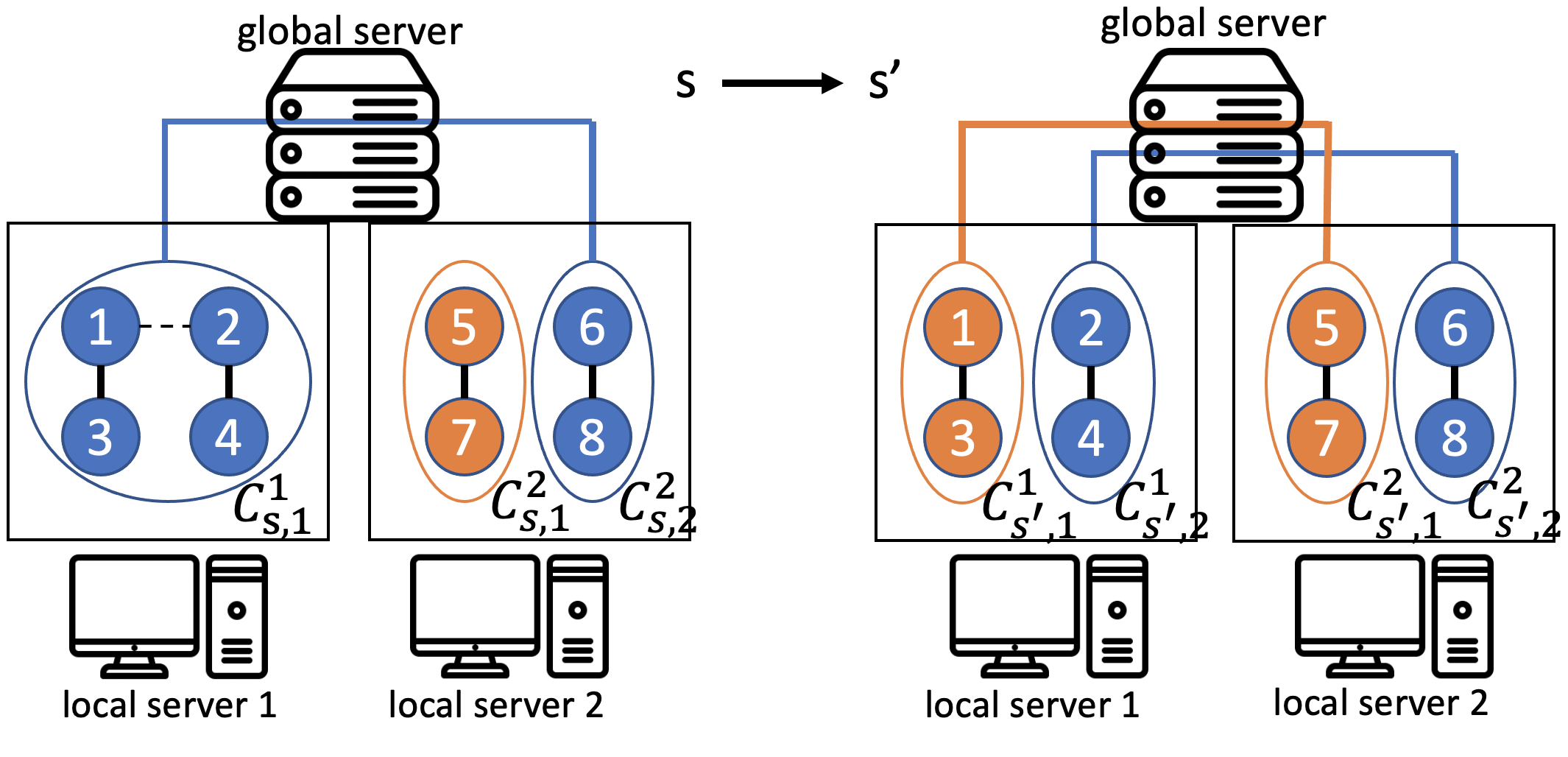
In this section, we introduce our phase-based federated clustering of bandit algorithms with CDP (FCLUB-CDP).

Identify the Underlying Cluster Structure. To correctly identify the cluster structure, we design a phase-based clustering detection algorithm in Algorithm 2. The high level idea is to first conduct local-level clustering of bandits on each local server and merge the local clusters on the global server.

At the local level, each server $\ell$ maintains a profile of $(\bm{V}_{t,i},\bm{b}_{t,i},T_{t,i})$ for its own local users $i\in\mathcal{U}^{\ell}$, where $V_{t,i}$ is Gramian matrix, $\bm{b}_{t,i}$ is the moment vector of regressand by the regressors, and $T_{t,i}$ is the number of times that $i$ has appeared up to time $t$. At the beginning of $s$ phase (or $t=2^{s}+1$), based on profiles $(\bm{V}_{t,i},\bm{b}_{t,i},T_{t,i})_{i\in\mathcal{U}^{\ell}}$, each server $\ell$ maintains an undirected graph structure $\mathcal{G}^{\ell}_{s}$, where nodes represent all local users $\mathcal{U}^{\ell}$ and a pair of users are connected by an edge if they are similar. We initialize the graph by a complete graph $\mathcal{G}^{\ell}_{0}$ and gradually delete edges at every beginning of each phase $s$. Specifically, in line 3, we delete edge between any user $i_{1}$ and $i_{2}$ if the distance between their estimated preference vector are larger than the following threshold.

where $\hat{\bm{\theta}}_{t,i}=(\lambda\bm{I}+\bm{V}_{t,i})^{-1}\bm{b}_{t,i}$ and $F(x)=\sqrt{\frac{1+\ln(1+x)}{(1+x)}}$. After the deletion, users in connected components $j\in C(\mathcal{G}^{\ell}_{s})$ are grouped into local cluster $j$. In line 5, server $\ell$ uploads the clustered information $I_{s,{\ell}}=(C^{\ell}_{s,j},\tilde{\bm{V}}^{\ell}_{s,j},\tilde{\bm{b}}^{\ell}_{s,j},\tilde{T}^{\ell}_{s,j})_{j\in C(\mathcal{G}^{\ell}_{s})}$ to the global server, which contains clustered information for each cluster $j\in C(\mathcal{G}^{\ell}_{s})$. Note that $I_{s,\ell}$ are added with random perturbation to protect the users’ data, which will be introduced shortly after.

In line 7, when the global server receives the privatized clustered information from all servers, it performs a merge operation to merge clusters from different servers whose estimated clustered preference vectors are close into a global clusters according to the following inequality.

where $\hat{\bm{\theta}}^{\ell}_{s,j}=(\tilde{\bm{V}}^{\ell}_{s,j})^{-1}\tilde{\bm{b}}^{\ell}_{s,j}$ and $F(x)=\sqrt{\frac{1+\ln(1+x)}{(1+x)}}$. $P_{s}$ denotes the set of $m_{s}$ global clusters. Note that the local clusters in the same global cluster indexed by $k\in[m_{s}]$ will communicate and share protected clustered information with each other in an asynchronous manner. At the beginning of phase $s$, if the new global cluster structure $P_{s}$ is different from $P_{s-1}$ at phase $s-1$, we will renew the shared global information $(\bm{S}^{g}_{t,k}$, $\bm{u}^{g}_{t,k}$, $T^{g}_{t,k})$ for $k\in[m_{s}]$. For local servers $(\ell,j)$ in the same global cluster $P_{s,k}$, the local synchronized information $(\bm{S}^{\ell}_{t,j},\bm{u}^{\ell}_{t,j},T^{\ell}_{t,j})$, the upload buffers $(\Delta\bm{S}^{\ell}_{t,j},\Delta\bm{u}^{\ell}_{t,j},\Delta T^{\ell}_{t,j})$ and download buffers $(\Delta\bm{S}^{-\ell}_{t,j},\Delta\bm{u}^{-\ell}_{t,j},\Delta T^{-\ell}_{t,j})$ are renewed. We also generate a new tree-based privatizer PVT$(\ell,j)$ for each cluster $j$ at server $\ell$, which will be introduced later on.

Asynchronous Communication Protocol. In this work, we design a novel asynchronous communication protocol to incorporate the randomly arriving users. To reduce the communication cost, our high-level idea is to use the delayed communication, where the feedback are temporarily stored in buffers and only if the stored information exceeds a threshold, the upload/download events are triggered. Such a threshold will ensure that the local information will not diverge too far from the global information, which in turn will not diverge too far from the scenario when information are fully synchronized. Also note that our communication is conducted in the asynchronous manner at the local cluster level. In other words, all local clusters indexed by $(\ell,j)\in P_{s,k}$ will establish connection with each other within the global cluster $k$. For each local cluster $(\ell,j)$, it stores a local copy of the sufficient statistics $(\bm{S}^{\ell}_{t,j},\bm{u}^{\ell}_{t,j},T^{\ell}_{t,j})$ and a upload buffer $(\Delta\bm{S}^{\ell}_{t,j},\Delta\bm{u}^{\ell}_{t,j},\Delta T^{\ell}_{t,j})$. For the global server, it prepares for each local cluster $(\ell,j)$ a download buffer $(\Delta\bm{S}^{-\ell}_{t,j},\Delta\bm{u}^{-\ell}_{t,j},\Delta T^{-\ell}_{t,j})$, which are used to send other local servers’ information to the local cluster. It also maintains the global statistics $(\bm{S}^{g}_{t,k},\bm{u}^{g}_{t,k},T^{g}_{t,k})$ to save the data uploaded from local clusters in global cluster $k$.

Our proposed communication framework consists of two components: the upload protocol (Algorithm 3) and the download protocol (Algorithm 4). For the upload protocol, at each time step $t$, user $i_{t}$ visits the server $l_{t}$ and receives recommended item $\bm{x}_{t}$. After the user $i_{t}$ interacts with the environment and observes feedback $(\bm{x}_{t},y_{t})$, the local server updates the upload buffers in line 1 and checks the following condition to decide whether to upload the upload buffer:

where $\bm{H}^{l_{t}}_{t,j_{t}}$ and $\bar{\bm{H}}^{l_{t}}_{t,j_{t}}$ are tentative and current perturbation for privacy protection, respectively. If the condition is satisfied, the local server sends $(\Delta\bm{S}^{l_{t}}_{t,j_{t}},\bm{u}^{l_{t}}_{t,j_{t}},T^{l_{t}}_{t,j_{t}})$ to the global cluster $k_{t}$. The global server then merges the uploaded information into the global information in line 4 and also sends it to download buffers for other local clusters $(\ell,j)\neq(l_{t},j_{t})\in P_{s,k_{t}}$ in line 6. For local cluster $(l_{t},j_{t})$ itself, the local server updates the local statistics and initializes the upload buffer using the newly generated perturbation in lines 8 to 10. For the download protocol, at each time step $t$, the global server will check the deviation between global statistics and the local statistics via following condition:

independently for local clusters $(\ell,j)$ in global cluster $P_{s,k_{t}}$. If any cluster $(\ell,j)$ satisfies such condition, the global server sends the information from other clusters to $(\ell,j)$, which is used to update $(\ell,j)$’s local statistics. Finally, the global server cleans the download buffer.

Tree-Based Privacy Protocol. To ensure the uploaded information are privatized, we adopt the tree-based privatizer to generate random perturbations $\bm{H}^{\ell}_{t,j}$ and $\bm{h}^{\ell}_{t,j}$ whenever an upload event happens. Note that the privatier subroutine is at the local cluster level and a new privatizer is created if the cluster structure changes at the start of any phase $s$.

Let $\bm{x}_{1},...,\bm{x}_{T}$ be a (matrix-valued) sequence of length $T$, and $s_{i}=\sum_{t=1}^{i}\bm{x}_{i}$ be the partial sum of the first $i$ elements that will be realised privately. Generally speaking, the tree-based mechanism Dwork et al. 2006 maintains a binary tree $\mathcal{T}$ of depth $1+\lceil\log T\rceil$, where the leaf nodes contain the elements $\bm{x}_{i}$ and the parent node maintains the sum of its children. For each node with value $n_{i}$, the tree-base mechanism protects privacy by adding noise $h_{i}$ to each node and release $n_{i}+h_{i}$ if queried. The key advantage is that such a tree only accesses $\nu=O(\log T)$ nodes to compute and release the partial sum $s_{i}$, which means the perturbation is at most $O(\nu)$ instead of $O(T)$.

Following this general idea, we implement the tree-based privatizer $(\ell,j)$ that satisfies the requirements of CDP. Recall that we only need to protect the information uploaded to the global server, it suffices to maintain a tree $\mathcal{T}^{\ell}_{j}$ of depth $\nu=O(1+\lceil\log t_{c}\rceil)$ for the upload event, where $t_{c}$ is the total number of uploads. To make the partial sums private, we insert a random noise matrix to each node in $\mathcal{T}^{\ell}_{j}$, similar to that of Shariff and Sheffet 2018 and Dubey and Pentland 2020,. Specifically, we sample a random matrix $\bar{\bm{N}}\in\mathbb{R}^{(d+1)\times(d+1)}$ where each entry $\bar{N}_{p,q}$ is drawn from i.i.d. Gaussian distribution $\mathcal{N}(0,\sigma_{\text{noise}})$ and symmetrize it to get $N=(\bar{\bm{N}}^{\top}+\bar{\bm{N}})/\sqrt{2}$. It follows that in order to ensure the whole tree is $(\varepsilon,\delta)$-DP, each node should preserve $(\varepsilon/\sqrt{8\nu\log(2/\delta}),\delta/2)$-DP. In other words, it suffices to set the variance $\sigma_{\text{noise}}=64\nu\log(2/\delta)^{2}/\epsilon^{2}$ for each tree node. Note that at each upload round $t$, the total noise added to the partial sum is the summation of at most $\nu$ random matrices with size $(d+1)\times(d+1)$, where the top-left $(d\times d)$-submatrix forms $\bm{H}^{\ell}_{t,j}$ and the first $d$ elements from the right-most $(d+1)\times 1$ vector forms $\bm{h}^{\ell}_{t,j}$. By concentration of random matrices Tao 2011, we have with probability at least $(1-\frac{\alpha}{mL})$, the operator norm of $\bm{H}^{\ell}_{t,j}$ is

for any $\ell\in[L],j\in[m],t\in[T]$.

Recommendation Procedure. At each time step $t$, the recommended item $\bm{x}_{t}$ for user $i_{t}$ is selected as follows. When the current cluster is correct (which is guaranteed after $O(\log T)$ rounds and to be proved later), the estimated $\hat{\bm{\theta}}_{t}=(\bm{S}^{l_{t}}_{t,j_{t}})^{-1}\bm{u}^{l_{t}}_{t,j_{t}}$ is computed using the local information $\bm{S}^{l_{t}}_{t,j_{t}}$ and $\bm{u}^{l_{t}}_{t,j_{t}}$. Since by Lemma 1, $\left\lVert\bm{\theta}_{i_{t}}-\hat{\bm{\theta}}_{t}\right\rVert_{2}\leq\beta^{l_{t}}_{t,j_{t}}$, the confidence radius is $\beta^{l_{t}}_{t,j_{t}}\left\lVert\bm{x}\right\rVert_{(\bm{S}^{l_{t}}_{t,j_{t}})^{-1}}$, which characterizes the exploration bonus for item $\bm{x}\in\bm{D}_{t}$. Then the local server will recommend the item $\bm{x}_{t}\in\bm{D}_{t}$ that maximizes the $\bm{x}^{\top}\hat{theta}_{t}$ plus the above exploration bonus. Finally, the user will receive feedback $y_{t}$ and the system updates corresponding statistics for better decision in future rounds.

Recall that perturbations $\bar{\bm{H}}^{\ell}_{t,j},\bar{\bm{H}}^{\ell}_{t,j}$ are designed to satisfy the $(\varepsilon,\delta,L,m)$-CDP requirement. In particular, the privacy budget $(\varepsilon,\delta)$ affects the regret and communication bounds via the following quantities $(\rho_{\max},\rho_{\min},\kappa)$, which can be treated as spectral bounds for $\bar{\bm{H}}^{\ell}_{t,j},\bar{\bm{H}}^{\ell}_{t,j}$. Let $\tilde{\bm{H}}^{\ell}_{t,j}=2\rho\bm{I}+3\rho c^{\ell}_{j,t}\bm{I}+\bar{\bm{H}}^{\ell}_{t,j}$, where $c^{\ell}_{j,t}$ is the number of uploads for local server $\ell$ and cluster $j$.

with probability at least $(1-\frac{\alpha}{mL})$.

As will be shown later, our communication protocol ensures $c^{\ell}_{j,t}\in[0,d\log T/\log(\min\{U,D\})]$, so $\rho_{\min}=\rho$, $\rho_{\max}=3\rho+3\rho d\log T/\log(\min\{U,D\})$ , and $\kappa=\left\lVert\bar{\bm{h}}^{\ell}_{t,j}\right\rVert/\sqrt{\rho}$, where $\rho\triangleq 8\sqrt{2}\nu\log(4/\delta)(4\sqrt{d}+2\log(2mL/\alpha))/\varepsilon$ is given by our privatizer.

In the following, we will give general regret and communication bounds using $(\rho_{\max},\rho_{\min},\kappa)$ and replace them with their exact values.

References

- Abbasi-Yadkori et al. [2011] Yasin Abbasi-Yadkori, Dávid Pál, and Csaba Szepesvári. Improved algorithms for linear stochastic bandits. Advances in neural information processing systems, 24:2312–2320, 2011.
- Anandkumar et al. [2011] Animashree Anandkumar, Nithin Michael, Ao Kevin Tang, and Ananthram Swami. Distributed algorithms for learning and cognitive medium access with logarithmic regret. IEEE Journal on Selected Areas in Communications, 29(4):731–745, 2011.
- Auer et al. [2002] Peter Auer, Nicolo Cesa-Bianchi, and Paul Fischer. Finite-time analysis of the multiarmed bandit problem. Machine learning, 47(2-3):235–256, 2002.
- Bistritz and Leshem [2018] Ilai Bistritz and Amir Leshem. Distributed multi-player bandits-a game of thrones approach. Advances in Neural Information Processing Systems, 31, 2018.
- Boursier and Perchet [2019] Etienne Boursier and Vianney Perchet. Sic-mmab: synchronisation involves communication in multiplayer multi-armed bandits. Advances in Neural Information Processing Systems, 32, 2019.
- Chan et al. [2011] T-H Hubert Chan, Elaine Shi, and Dawn Song. Private and continual release of statistics. ACM Transactions on Information and System Security (TISSEC), 14(3):1–24, 2011.
- Chu et al. [2011] Wei Chu, Lihong Li, Lev Reyzin, and Robert Schapire. Contextual bandits with linear payoff functions. In Proceedings of the Fourteenth International Conference on Artificial Intelligence and Statistics, pages 208–214. JMLR Workshop and Conference Proceedings, 2011.
- Dani et al. [2008] Varsha Dani, Thomas P Hayes, and Sham M Kakade. Stochastic linear optimization under bandit feedback. 2008.
- Dubey and Pentland [2020] Abhimanyu Dubey and AlexSandy’ Pentland. Differentially-private federated linear bandits. Advances in Neural Information Processing Systems, 33:6003–6014, 2020.
- Dwork et al. [2006] Cynthia Dwork, Frank McSherry, Kobbi Nissim, and Adam Smith. Calibrating noise to sensitivity in private data analysis. In Theory of cryptography conference, pages 265–284. Springer, 2006.
- Gentile et al. [2014] Claudio Gentile, Shuai Li, and Giovanni Zappella. Online clustering of bandits. In International Conference on Machine Learning, pages 757–765. PMLR, 2014.
- Gentile et al. [2017] Claudio Gentile, Shuai Li, Purushottam Kar, Alexandros Karatzoglou, Giovanni Zappella, and Evans Etrue. On context-dependent clustering of bandits. In International Conference on Machine Learning, pages 1253–1262. PMLR, 2017.
- Kairouz et al. [2021] Peter Kairouz, H Brendan McMahan, Brendan Avent, Aurélien Bellet, Mehdi Bennis, Arjun Nitin Bhagoji, Kallista Bonawitz, Zachary Charles, Graham Cormode, Rachel Cummings, et al. Advances and open problems in federated learning. Foundations and Trends® in Machine Learning, 14(1–2):1–210, 2021.
- Korda et al. [2016] Nathan Korda, Balazs Szorenyi, and Shuai Li. Distributed clustering of linear bandits in peer to peer networks. In International conference on machine learning, pages 1301–1309. PMLR, 2016.
- Lattimore and Szepesvári [2020] Tor Lattimore and Csaba Szepesvári. Bandit Algorithms. Cambridge University Press, 2020.
- Li and Wang [2021] Chuanhao Li and Hongning Wang. Asynchronous upper confidence bound algorithms for federated linear bandits. arXiv preprint arXiv:2110.01463, 2021.
- Li et al. [2010] Lihong Li, Wei Chu, John Langford, and Robert E Schapire. A contextual-bandit approach to personalized news article recommendation. In Proceedings of the 19th international conference on World wide web, pages 661–670, 2010.
- Li and Zhang [2018] Shuai Li and Shengyu Zhang. Online clustering of contextual cascading bandits. In Thirty-Second AAAI Conference on Artificial Intelligence, 2018.
- Li et al. [2016] Shuai Li, Alexandros Karatzoglou, and Claudio Gentile. Collaborative filtering bandits. In Proceedings of the 39th International ACM SIGIR conference on Research and Development in Information Retrieval, pages 539–548, 2016.
- Li et al. [2019] Shuai Li, Wei Chen, and Kwong-Sak Leung. Improved algorithm on online clustering of bandits. arXiv preprint arXiv:1902.09162, 2019.
- Li et al. [2021] Ye Li, Hong Xie, Yishi Lin, and John CS Lui. Unifying offline causal inference and online bandit learning for data driven decision. In Proceedings of the Web Conference 2021, pages 2291–2303, 2021.
- Rosenski et al. [2016] Jonathan Rosenski, Ohad Shamir, and Liran Szlak. Multi-player bandits–a musical chairs approach. In International Conference on Machine Learning, pages 155–163. PMLR, 2016.
- Shariff and Sheffet [2018] Roshan Shariff and Or Sheffet. Differentially private contextual linear bandits. arXiv preprint arXiv:1810.00068, 2018.
- Shi and Shen [2021] Chengshuai Shi and Cong Shen. Federated multi-armed bandits. In Proceedings of the 35th AAAI Conference on Artificial Intelligence (AAAI), 2021.
- Tao [2011] Terence Tao. Topics in random matrix theory. Graduate Studies in Mathematics, 132, 2011.
- Zhang et al. [2020] Xiaoying Zhang, Hong Xie, Hang Li, and John CS Lui. Conversational contextual bandit: Algorithm and application. In Proceedings of The Web Conference 2020, pages 662–672, 2020.
- Zheng et al. [2020] Kai Zheng, Tianle Cai, Weiran Huang, Zhenguo Li, and Liwei Wang. Locally differentially private (contextual) bandits learning. arXiv preprint arXiv:2006.00701, 2020.
- Zhu et al. [2021] Zhaowei Zhu, Jingxuan Zhu, Ji Liu, and Yang Liu. Federated bandit: A gossiping approach. In Abstract Proceedings of the 2021 ACM SIGMETRICS/International Conference on Measurement and Modeling of Computer Systems, pages 3–4, 2021.
Supplementary Material
Appendix A Summary of Notations