Finding Near-Optimal Weight Independent Sets at Scale
Abstract.
Computing maximum weight independent sets in graphs is an important NP-hard optimization problem. The problem is particularly difficult to solve in large graphs for which data reduction techniques do not work well. To be more precise, state-of-the-art branch-and-reduce algorithms can solve many large-scale graphs if reductions are applicable. Otherwise, their performance quickly degrades due to branching requiring exponential time. In this paper, we develop an advanced memetic algorithm to tackle the problem, which incorporates recent data reduction techniques to compute near-optimal weighted independent sets in huge sparse networks. More precisely, we use a memetic approach to recursively choose vertices that are likely to be in a large-weight independent set. We include these vertices into the solution, and further reduce the graph. We show that identifying and removing vertices likely to be in large-weight independent sets opens up the reduction space and speeds up the computation of large-weight independent sets remarkably. Our experimental evaluation indicates that we are able to outperform state-of-the-art algorithms. For example, our two algorithm configurations compute the best results among all competing algorithms for 205 out of 207 instances. Thus can be seen as a useful tool when large-weight independent sets need to be computed in practice.
1. Introduction
For a given graph an independent set (IS) is defined as a subset of all vertices such that each pair of vertices in are non adjacent. A maximum independent set (MIS) describes an IS with highest possible cardinality. By transforming the graph into the complement graph the MIS problem results in the maximum clique problem. However, for sparse graphs , using a maximum clique solver is impractical as the complement is very dense and therefore unlikely to fit in memory for all but the smallest instances. Another related problem is the minimum vertex cover problem. Note that for a MIS of , is a minimum vertex cover. For a weighted graph with non-negative vertex weights given by a function , the maximum weight independent set (MWIS) problem is to find an independent set with maximum weight . The applications of the MWIS problem, as well as the related problems addressed above, can be used for solving different application problems such as long-haul vehicle routing (Dong et al. 2022), the winner determination problem (Wu and Hao 2015) or prediction of structural and functional sites in proteins (Mascia et al. 2010). As a detailed example, consider an application of MWIS for map labeling, where displaying non-overlapping labels throughout dynamic map operations such as zooming and rotating (Gemsa et al. 2016) or while tracking a physical movement of a user or set of moving entities (Barth et al. 2016) is of high interest in many applications. In the underlying map labeling problem, the labels are represented by vertices in a graph, weighted by importance. Each pair of vertices is connected by an edge if the two corresponding labels would overlap. In this graph, a MWIS describes a high-quality set of labels, with regard to their importance level, that can be visualized without any overlap.
Since these problems are NP-hard (Garey and Johnson 1979), heuristic algorithms are used in practice to efficiently compute solutions of high quality on large graphs (Andrade et al. 2012; Grosso et al. 2008; Xiao et al. 2021). Depending on the definition of the neighborhood, local search algorithms are able to explore local solution spaces very effectively. However, local search algorithms are also prone to get stuck in local optima. As with many other heuristics, results can be improved if several repeated runs are made with some measures taken to diversify the search. Still, even a large number of repeated executions can only scratch the surface of the huge space of possible independent sets for large-scale data sets.
Traditional branch-and-bound methods (San Segundo et al. 2013; San Segundo et al. 2011; Tomita et al. 2010; Gellner et al. 2021; Lamm et al. 2019; Hespe et al. 2020) may often solve small graphs with hundreds to thousands of vertices in practice, and medium-sized instances can be solved exactly in practice using reduction rules to reduce the graph. In particular, it has been observed that if data reductions work very well, then the instance is likely to be solved. If data reductions do not work very well, i.e. the size of the reduced graph is large, then the instance can often not be solved. Even though new algorithms such as the struction algorithm (Gellner et al. 2021) already manage to solve a lot of large instances, some remain unsolved.
In order to explore the global solution space extensively, more sophisticated metaheuristics, such as GRASP (Dong et al. 2022) or iterated local search (Andrade et al. 2012; Nogueira et al. 2018), have been used. In this work, we extend the set of metaheuristics used for the MWIS problem by introducing a novel memetic algorithm. Memetic algorithms (MAs) combine genetic algorithms with local search (Kim et al. 2011) to effectively explore (global search) and exploit (local search) the solution space. The general idea behind genetic algorithms is to use mechanisms inspired by biological evolution such as selection, mutation, recombination, and survival of the fittest.
Our Results.
Our contribution is two-fold: First, we develop a state-of-the-art memetic algorithm that is based on recombination operations employing graph partitioning techniques. It computes large-weight independent sets by incorporating a wide range of recently developed advanced reduction rules. In particular, our algorithm uses a wide range of frequently used data reduction techniques from (Lamm et al. 2019; Gellner et al. 2021) and also employs a number of recently proposed data reduction rules by Gu et al. (Gu et al. 2021).
The algorithm may be viewed as performing two functions simultaneously: (1) reduction rules for the weighted independent set problem are used to boost the performance of the memetic algorithm and (2) the memetic algorithm opens up the opportunity for further reductions by selecting vertices that are likely to be in large-weight independent sets. In short, our method applies reduction rules to form a reduced graph, then computes vertices to insert into the final solution and removes their neighborhood (including the vertices themselves) from the graph. Thus further reductions can be applied. The process is then repeated recursively until the graph is empty. We show that this technique finds near-optimal weighted independent sets much faster than existing local search algorithms, is competitive with state-of-the-art exact algorithms for smaller graphs, and allows us to compute large-weight independent sets on huge sparse graphs. Overall, our algorithm configurations compute the best results among all competing algorithms for 205 out of 207 instances, and thus can be seen as the dominating tool when large weight independent sets need to be computed in practice.
Our second contribution in this work is the experimental evaluation of the orderings in which currently available data reductions are applied. We examine the impact of different orderings on solution size and on running time. One outcome of this evaluation are robust orderings of reductions for exact reduction rules, as well as a specific ordering which can improve the solution quality further at an expense of computation time.
2. Preliminaries
In this work, a graph is an undirected graph with and , where . The neighborhood of a vertex is defined as . Additionally, . The same sets are defined for the neighborhood of a set of vertices , i.e. and . The degree of a vertex is defined as the number of its neighbors . The complement graph is defined as , where is the set of edges not present in . A set is called independent set (IS) if for all vertices there is no edge . For a given IS a vertex is called free, if is still an independent set. An IS is called maximal if there are no free vertices. The maximum independent set problem (MIS) is that of finding an IS with maximum cardinality. The maximum weight independent set problem (MWIS) is that of finding an IS with maximum weight. The weight of an independent set is defined as and describes the weight of a MWIS of the corresponding graph. The complement of an independent set is a vertex cover, i.e. a subset such that every edge is covered by at least one vertex . An edge is covered if it is incident to one vertex in the set . The minimum vertex cover problem, defined as looking for a vertex cover with minimum cardinality, is thereby complementary to the MIS problem. Another closely related concept are cliques. A clique is a set such that all vertices are pairwise adjacent. A clique in the complement graph corresponds to an independent set in the original graph . A vertex is called isolated or simplicial, when its neighborhood forms a clique.
The subdivision of the set of vertices into disjoint blocks , such that is called a -way partition (see (Schulz and Strash 2019; Çatalyürek et al. 2022)). To ensure the blocks to be roughly of the same size, the balancing constraint with the imbalance parameter is introduced. While satisfying this balance constraint, the edge separator problem asks for minimizing the total cut, , where is defined by . The edge separator is the set of all edges in the cut. For the -vertex separator problem on the other hand we look for a division of into blocks. In addition to the blocks a separator exists. This separator has to be chosen such that no edges between the blocks exist, but there is no balancing constraint on the separator . However, as for the edge separator problem the balancing constraint on the blocks has to hold. To solve the problem, the size of the separator has to be minimized. By removing the separator from the graph it results in at least connected components, since the different blocks are not connected.
3. Related Work
Here we give only a short overview of existing exact and heuristic techniques; for more details, see the expanded discussion in Appendix A or the recent survey on practical data reduction (Abu-Khzam et al. 2022).
3.1. Exact Methods
Exact algorithms usually compute optimal solutions by systematically exploring the space of solutions via variations of branch-and- bound (Östergård 2002; Warren and Hicks 2006). Branching schemes and better pruning methods use upper and lower bounds to exclude specific subtrees (Balas and Yu 1986; Babel 1994; Li et al. 2017b). Of note, Warren and Hicks (Warren and Hicks 2006) proposed three branch-and-bound algorithms that use weighted clique covers as an upper bound, using a branching scheme first introduced by Balas and Yu (Balas and Yu 1986).
Data reduction rules are frequently intermixed with branching and bounding, yielding so-called branch-and-reduce algorithms (Akiba and Iwata 2016), which can improve their worst-case (and practical) running time. For the unweighted case, many branch-and-reduce algorithms have been developed. In 2019 reduction rules for the MWIS problem were introduced, resulting in the first branch-and-reduce algorithm for MWIS by Lamm et al. (Lamm et al. 2019). They first introduce data reductions, together with a branch-and-reduce algorithm using pruning with weighted clique covers (Warren and Hicks 2006) for upper bounds and an adapted version of the ARW local search (Andrade et al. 2012) for lower bounds.
Since this result, many new data reductions and branch-and-reduce algorithms have been introduced. Gellner et al. (Gellner et al. 2021) integrated variants of the struction reduction (Ebenegger et al. 1984; Alexe et al. 2003) that may increase the graph size. Recently, Xiao et al. (Xiao et al. 2021) and Zheng et al. (Zheng et al. 2020) presented further data reductions and simple exact algorithms based on these data reduction rules and Huang et al. (Huang et al. 2021) proposed a branch-and-reduce algorithm for maximum weight independent set with running time .
Finally, there are exact procedures which are either based on other extension of the branch-and-bound paradigm (Rebennack et al. 2011; Warrier et al. 2005; Warrier 2007), or on the reformulation into other -complete problems, such as SAT, for which a variety of solvers already exist (Xu et al. 2016).
We additionally note that there are several recent works on the complementary maximum weighted clique problem that are able to handle large real-world networks (Fang et al. 2016; Jiang et al. 2017; Held et al. 2012). However, using these solvers for the MWIS problem require computing complement graphs. Since large real-world networks are often very sparse, processing their complements quickly becomes infeasible due to their memory requirement.
3.2. Heuristic Methods
A widely used heuristic approach is local search, which usually computes an initial solution and then tries to improve it by simple insertion, removal or swap operations. Although local search generally offers no guarantees for solution quality, in practice local search algorithms find high-quality solutions significantly faster than exact procedures.
For unweighted graphs, the iterated local search (ARW) by Andrade et al. (Andrade et al. 2012), is a very successful heuristic. It is based on so-called -swaps which remove one vertex from the solution and add two new vertices to it, thus improving the current solution by one. Their algorithm is able to find (near-)optimal solutions for small to medium-size instances in milliseconds, but struggles on massive instances with millions of vertices and edges.
The hybrid iterated local search (HILS) by Nogueira et al. (Nogueira et al. 2018) adapts the ARW algorithm for weighted graphs. In addition to weighted -swaps, it also uses -swaps that add one vertex into the current solution and exclude its neighbors.
Two other local searches, DynWVC1 and DynWVC2, for the equivalent minimum weight vertex cover problem are presented by Cai et al. (Cai et al. 2018). In practice, DynWVC1 outperforms previous MWVC heuristics on map labeling instances and large scale networks, and DynWVC2 provides further improvements on large scale networks but performs worse on map labeling instances.
Li et al. (Li et al. 2019) presented a local search algorithm for the MWVC problem that applies reduction rules during the construction phase of the initial solution. Experiments show that their algorithm outperforms state-of-the-art approaches on graphs of up to millions of vertices and on real-world instances.
Recently, a new hybrid method for MWVC was introduced by Langedal et al. (Langedal et al. 2022), combining elements from exact methods with local search, data reductions and graph neural networks. In their experiments they achieve improvements compared to DynWVC2 and HILS in both solution quality and running time.
Lamm et al. (Lamm et al. 2015) presented an evolutionary approach, EvoMIS, to tackle the MIS problem. ReduMIS by Lamm et al. (Lamm et al. 2017) combines branch-and-reduce approach with EvoMIS. In their experiments, ReduMIS outperformed the local search ARW as well as the pure evolutionary approach EvoMIS.
Another reduction based heuristic called HtWIS was presented recently by Gu et al. (Gu et al. 2021). They repeatedly apply the following steps until reaching an empty graph. First they reduce exhaustively and then choose one vertex by a tie-breaking policy to add to the solution. Now this vertex as well as its neighbors can be removed from the graph and the reductions can be applied again. Their experiments prove a significant improvement in running time as well as solution quality compared to state-of-the-art solvers.
Recently, a new metaheuristic was introduced by Dong et al. (Dong et al. 2022) in particular for vehicle routing instances. With their algorithm METAMIS they developed a new local search algorithm combining a wide range of simple local search operations with a new variant of path-relinking to escape local optima. In their experiments they outperform HILS algorithm on a wide range of instances both in time and solution quality.
4. Algorithm
We now present our memetic algorithm for the MWIS problem, which we call memetic maximum weight independent set m2wis. This algorithm is inspired by ReduMIS (Lamm et al. 2017) and works in rounds, where each round can be split up into three parts. In the beginning of each round the exact reduction step takes place. Here the graph is reduced as far as possible using a wide range of data reduction rules. On the resulting reduced graph, we apply the memetic part of the algorithm as the second step. We represent a solution, also referred to as an individual, by using bitvectors. Meaning the independent set is represented as an array . For each array entry it holds iff . The memetic component itself works in rounds as well. Starting with an initial population , consisting of a set of individuals, this population is evolved over several rounds until a stopping criterion is fulfilled. In the third part, we select a subset of vertices to be included in the independent set by considering the resulting population. Here, we implement different strategies to select vertices for inclusion. Including these vertices in the independent set enables us to remove them and their neighbors from the instance. This breaks up the reduction space, i.e. further reductions might be applicable after the removal process. The steps of exact reduction, memetic search, and heuristic reduction are repeated until the remaining graph is empty or another stopping criterion is fulfilled.
Following the order of the Algorithm 1, we first describe the ExactReduce routine in Section 4.1. Section 4.2 is devoted to the memetic part, followed by the description of different vertex selection strategies used to heuristically reduce the instance and open up the reduction space in Section 4.3.
4.1. Exact Reductions
Especially for large instances, applying exact data reductions is a very important technique to reduce the problem size. In general, reductions allow the identification of vertices (1) as part of a solution to the MWIS problem, (2) as non-solution vertices or (3) as deferred, meaning the decision for this vertex is depending on additional information about neighboring vertices that will be obtained later. The resulting reduced graph, after no reduction rule can be applied anymore we denote by . Once a solution on is found, reductions can be undone to reconstruct a MWIS on the original graph. For the reduction process we apply a large set of reductions which we list here.
Case 1:

Case 2:

Case 3:

In the following list of reductions refers to a MWIS of , refers to a MWIS of the modified graph .
Reduction 1 (Neighborhood Removal (Lamm et al. 2019)).
For any , if then is in some MWIS of . Let and .
Reduction 2 (Degree-One (Gu et al. 2021)).
Let be a degree-one vertex with the neighbor in .
- •
Case 1: if , must be contained in some MWIS of ; thus can be removed from , i.e. , where is the graph obtained by removing both and .
- •
Case 2: if , , where is the graph obtained by removing and updating the weight of to be . It holds that iff .
We note that Case 1 is a special case of Reduction 1.
Reduction 3 (Triangle (Gu et al. 2021)).
This reduction is illustrated in Figure 1. Let be a degree-two vertex with two neighbors and in , where edge . Without loss of generality, assume .
- •
Case 1: if , must be contained in some MWIS of . This leads to , where is obtained by removing , , .
- •
Case 2: if , , where is the graph obtained by removing nodes and , and updating . It holds that iff .
- •
Case 3: if , , where is the graph obtained by removing , and updating as well as . It holds for that iff .
Reduction 4 (Extended V-Shape (Lamm et al. 2019; Gu et al. 2021)).
Let be a degree-two vertex with the neighbors and in , where edge . Without loss of generality, assume .
- •
Case 1: (Lamm et al. 2019) if
- –
if , must be contained in some MWIS of and this leads to , where is obtained by removing .
- –
else we fold into a vertex with weight forming a new graph . Then . If then , otherwise . It holds that iff ;
- –
- •
Case 2: (Gu et al. 2021) if , , where is the graph obtained by removing , updating and . It holds that , iff ;
- •
Case 3: (Gu et al. 2021) if , , where is the graph obtained by updating , , and . It holds that iff .
Reduction 5 (Isolated Vertex Removal (Lamm et al. 2019)).
Let be isolated and . Then is in some MWIS of . Let and .
Reduction 6 (Basic Single-Edge (Gu et al. 2021)).
Given an edge , if , it holds that , where is obtained by removing from .
Reduction 7 (Extended Single-Edge (Gu et al. 2021)).
For an edge with , it holds that , where is obtained by removing all vertices in .
Reduction 8 (Domination (Lamm et al. 2019)).
Let be vertices such that (i.e., dominates ). If , there is an MWIS in that excludes and . Therefore, can be removed from the graph.
Reduction 9 (Twin (Lamm et al. 2019)).
Let vertices and have equal neighborhoods , forming an independent set. We have two cases:
- (1)
If , then and are in some MWIS of . Let .
- (2)
If , but , then we can fold into a new vertex with weight and call this graph . Then we construct an MWIS of as follows: if then , if then .
Furthermore, .
Reduction 10 (Simplicial Weight Transfer (Lamm et al. 2019)).
Let be isolated, and suppose that the set of simplicial vertices is such that , . We
- (1)
remove all such that , and let the remaining neighbors be denoted by ,
- (2)
remove and set its new weight to , and
let the resulting graph be denoted by . Then and an MWIS of can be constructed from an MWIS of as follows: if then , otherwise .
Reduction 11 (CWIS (Butenko and Trukhanov 2007)).
Let be a critical weighted IS of , i.e. is an IS of . Then is in some MWIS of . We set and .
Reduction 12 (Neighborhood Folding (Lamm et al. 2019)).
Let , and suppose that is independent. If , but , then fold and into a new vertex with weight . If then , otherwise if then . Furthermore, .
In the ExactReduce routine, we test for each of these reductions whether they are applicable. This takes place in a predefined order. If one reduction is successfully applied, then the process of testing possible reductions starts from the beginning (according to this order). If no more reductions can be applied, we obtained the reduced graph and continue with the next part of Algorithm 1.
The order in which reductions are applied has an effect on the weight offset and the size of the resulting reduced graph, as well as on the time needed for the computation. We give a detailed analysis in Appendix B.
4.2. Memetic Algorithm
After ExactReduce, we apply the Evolve routine which is described in Algorithm 2 on the reduced graph . This starts by generating an initial population of size which we then evolve over several generational cycles (rounds). For the evolution of the population two individuals from the population are selected and combined to create an offspring. We also apply a mutation operation to this new solution by forcing new vertices into the solution and removing neighboring solution vertices. To keep the population size constant and still add a new offspring to the solution, we look for fit replacements. In this process, we search for individuals in the population, which have smaller weights than the new offspring. Among those, we look for the most similar solution by computing the intersection size of the new and existing individuals. We also added the possibility of forcing individuals into the population if it has not changed over a certain number of iterations, as well as rejecting the offspring if the solution with the smallest weight is still better than the new offspring. Note that the size of the population does not change during this process. Additionally, at any time the individuals of our population are forming an independent set. In the last step of the memetic algorithm we improve the solution by the HILS algorithm. The stopping criterion for the memetic procedure is either a specified number of unsuccessful combine operations or a time limit. In the following we discuss each of these steps in detail. We start with introducing the computation of the initial solution in Section 4.2.1 and then explain the combine operations for the evolutionary process in Section 4.2.2 as well as the mutation operation in Section 4.2.3.
4.2.1. Initial Solutions
At the start of our memetic algorithm, we create an initial population of size . To diversify as much as possible, this population contains solutions computed in six different ways, which we choose uniformly at random to create an individual. Before applying the strategies we permute the order of the nodes such that different solutions are obtained for the same strategy by different tie breaking.
RandomMWIS. The first approach works by starting with an empty solution and adding free vertices uniformly at random until the solution is maximal.
GreedyWeightMWIS. For the GreedyWeightMWIS strategy, we start with an empty solution. This is extended to a maximal independent set by adding free vertices ordered by their weight. Starting with the largest weight, we include this vertex and exclude all its neighbors until all vertices are labeled either included or excluded.
GreedyDegreeMWIS. Via this greedy approach, we create initial solutions by successively choosing the next free vertex with the smallest residual degree. Each time a vertex is included, we label the neighboring vertices to be excluded.
GreedyWeightVC. In contrast to the previous approaches, here the vertex cover problem, the complementary problem to the independent set problem, is utilized. Therefore, an empty solution is extended by vertices of the smallest weight until a vertex cover is computed. As soon as the algorithm terminated, we compute the complement and have an initial solution to the MWIS problem.
GreedyDegreeVC. As in GreedyWeightVC the complementary vertex cover problem is solved. However, for this approach, we choose those vertices to include in the solution, which cover the maximum number of currently uncovered edges.
CyclicFast. We also add the possibility to compute an initial solution via the CyclicFast algorithm by Gellner et al. (Gellner et al. 2021). We set a time limit of 60 seconds.
4.2.2. Combine Operations
The common idea of our combine operations is to combine whole blocks of independent set vertices. To construct those blocks, we use the graph partitioning framework KaHIP (Sanders and Schulz [n. d.]) which computes partitions of the graph . For the solution blocks are defined by . We created different offspring by using the following combine operations on those solution blocks.
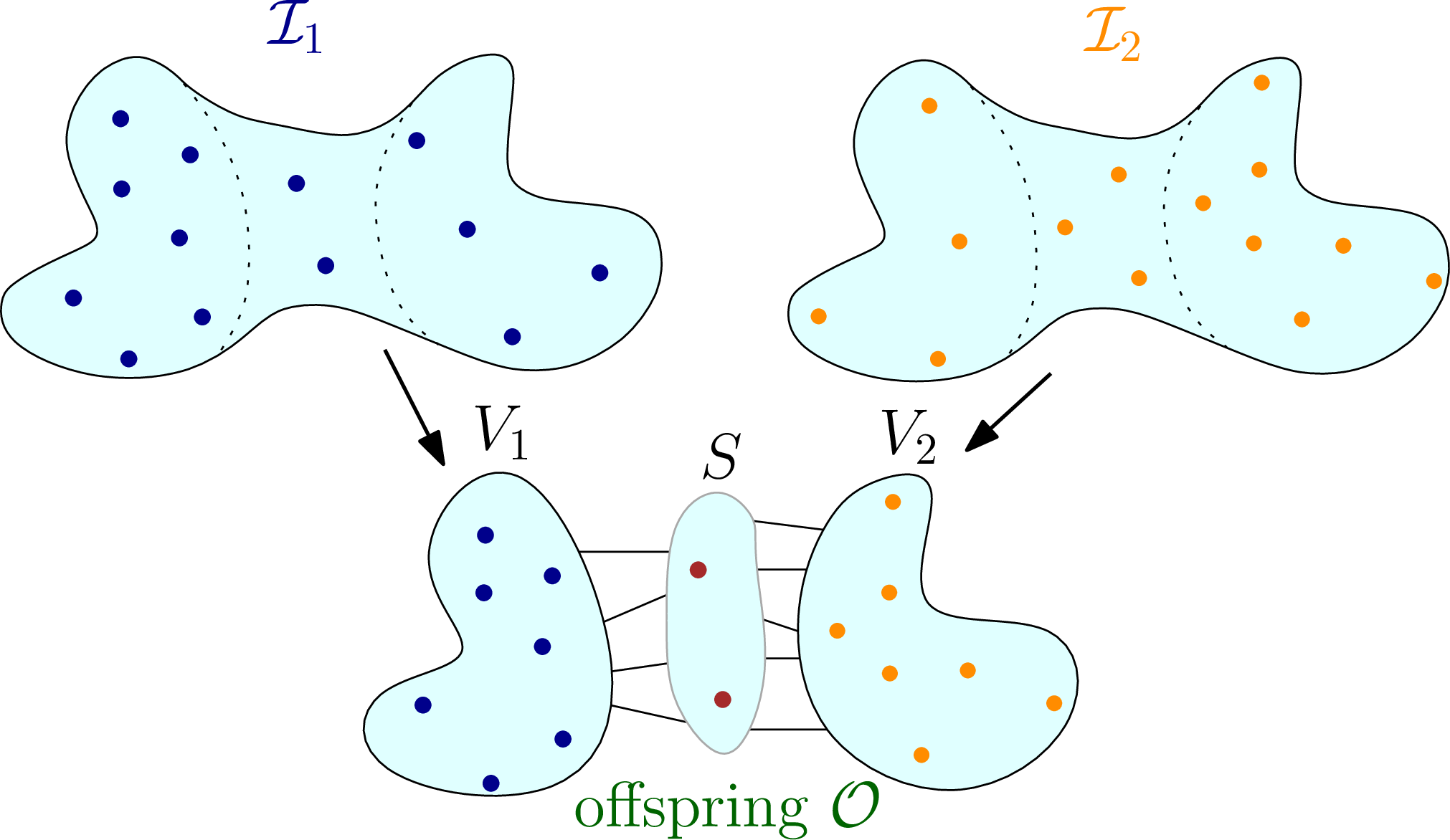
The parents for the first two combine operations are chosen by two runs of the tournament selection (Miller and Goldberg 1996), where the fittest individual i.e. the solution with highest weight gets selected out of two random individuals from the population. Then we perform one of the combine operations outlined below and finally, after the combine operation, we use the HILS algorithm (Nogueira et al. 2018) to improve the computed offspring.
Vertex Separator Combination.
The first operator works with a vertex separator . We use a vertex separator to be able to exchange whole blocks of solutions without violating the independent set property. This can be done because no vertices belonging to different blocks are adjacent to one another. Neighboring vertices would either be part of the same block or one of them has to belong to the separator . By this property the combination of those blocks will always result in a valid solution to the independent set problem. The two individuals selected by the tournament and are split up according to these partitions and then combined to generate two offspring and . After that we add as many free vertices greedily by weight until the solution is maximal, we get a local optimum via one iteration of the weighted local search. See Figure 2 for an illustration.
Multi-way Vertex Separator Combination.
We extended the previous described operator to the multi-way vertex separator, where multiple solutions can be used and combined. Therefore, we compute a -vertex separator and select individuals. Then for every pair of partition and individual for a score is computed. This score is defined by . We start with the pair resulting in the highest score pair and then select pairs decreasingly. Once an individual or partition block is selected, we do not use it again. In contrast to the previous operator, this combination only results in one offspring.We then maximize this offspring and compute a local maximum.
Edge Separator Combination.
For this operator we exploit the duality to the weighted vertex cover problem. Starting with a partition the operator computes temporary offspring for the weighted vertex cover problem. Let and be the individuals selected by the tournament rule. Let be the solution to the weighted vertex cover problem for . The new offspring are and . However, these offspring can contain some non-covered edges, which are a subset from the cut edges between the two partitions. The graph induced by the non-covered cut edges is bipartite. In this graph we compute a weighted vertex cover using maximum flows.
Multi-way Edge Separator Combination.
Similar to the vertex separator also the edge separator can be extended to use multiple solutions. Therefore, a -way-partition is computed. Equivalent to the multi-way vertex separator, we also select individuals and compute a score for each pair and . For the scoring function, the complement of an independent set inside the given block is used to sum up the weights of the vertices of the vertex cover in this block. For the offspring computation, each block is combined with the individual with the lowest score. As in the basic edge separator combine operator there can be edges in the cut that are not covered. Since the induced graph here is not bipartite we handle this problem using a simple greedy strategy. Afterwards the solution is transformed to get the offspring for the independent set individuals.
4.2.3. Mutation Operation
After each combine operation, a mutation operator can perturb the created offspring. This is done by forcing new vertices into the solution and removing the adjacent vertices to satisfy the independent set property. Those vertices are selected at random among all non solution nodes in the graph. Afterwards we improve the solution using the HILS algorithm.
4.3. Heuristic Reductions and Recursion
After the memetic algorithm stops, we use a heuristic data reduction to open up the reduction space (and afterwards the next round of exact data reductions begins). We implemented different strategies to select vertices that we put into the solution. In each strategy, vertices are ordered by a rating function. Depending on the configuration, the algorithm either inserts the best vertex or a set of vertices into the solution. We now explain the different selection strategies.
Vertex Selection by Weight.
The first rating function is based on the weight of a vertex (higher is better). The intuition here is that by adding a vertex, we want to increase the weight of our solution as much as possible. More precisely, the fittest individual from the population evolved by the memetic algorithm is selected. The fitness of an individual is defined as the solution weight. From this individual, we select the vertices from the independent set that have the highest weight and add them to our solution. Since we only consider vertices from one individual, can be freely chosen without violating the independent set property of our solution. For example, we can choose to only add the highest weight vertex or select a fraction of those solution vertices.
Vertex Selection by Degree.
Similar to the previous vertex selection strategy, we choose the fittest individual from which we add vertices to our solution. Here, the vertices are rated by their degree (smaller is better). The intuition here is that adding vertices with a small degree to our solution will not remove too many other vertices from the graph that could be considered later.
Vertex Selection by Weight/Degree.
For this selection strategy, we rate the vertices of the fittest individual by the fraction (higher is better). This way we combine the two previous ratings.
Hybrid Vertex Selection.
In the hybrid case, the solution vertices are rated by the weight difference between a vertex and its neighbors (higher is better). This value describes the minimum gain in solution weight we can achieve by adding the vertex to the solution. Note that Gu et al. (Gu et al. 2021) proposed this rule for their algorithm. The key difference here is that Gu et al. (Gu et al. 2021) use this function on all vertices, while our algorithm only considers solution vertices of the fittest solution of the memetic algorithm.
Vertex Selection by Solution Participation.
In contrast to the previous strategies, this strategy considers the whole population. Moreover, here we consider each vertex in the graph. We check the population and assign each vertex a value according to the number of times it is part of a solution. The maximum number a vertex can achieve is therefore bounded by the population size . Since many vertices achieved the same score, we subtracted for each vertex from the solution participation value for tie-breaking. Note that in this strategy we only add one vertex to the solution.
5. Experimental Evaluation
Methodology.
We implemented our algorithm using C++11. The code is compiled using g++ version 12.2 and full optimizations turned on (-O3). We compare our algorithm against the struction algorithm by Gellner et al. (Gellner et al. 2021) and the (more recent) algorithm HtWIS by Gu et al. (Gu et al. 2021). We also compare the results with the branch-and-reduce algorithm by Lamm et al. (Lamm et al. 2019), as well as the HILS algorithm by Nogueira et al. (Nogueira et al. 2018). In most cases HILS outperforms DynWVC1 and DynWVC2 (Lamm et al. 2019). Hence, we omit comparisons to DynWVC1 and DynWVC2. We generally run each configuration with four different seeds and a time limit of ten hours and report the mean results. If a solver exceeded a memory threshold of 100 GB during a time limit of 10h for an instance we note this with a dash. In general, our algorithm does not test the time limit in the ExactReduce routine of m2wis or during the calculation of the separator and partition pool. Hence, if the 10h mark is reached during these steps, the time limit can be exceeded. We used a machine equipped with a AMD EPYC 7702P (64 cores) processor and 1 TB RAM running Ubuntu 20.04.1. We used the fast configuration of the KaHIP graph partitioning package (Sanders and Schulz 2011; Sanders and Schulz 2016) for the computation of the graph partitions and vertex separators. We also present extensive experiments regarding the impact of reduction ordering. Due to space constraints we give the results in the Appendix B. We conclude that the order in which we introduce the reductions from Reduction 1 to Reduction 12 is already robust and hence use it for the remaining experiments.
Parameter Configuration.
We set up experiments to find good parameters for our algorithm. Here, we only show detailed analysis regarding the vertex selection strategy. In these previous experiments we found that increasing the amount of vertices added during HeuristicReduce reduces the total running time. However, since the solution quality decreases as well, we focus on only adding one vertex during HeuristicReduce in all following experiments for m2wis. Similar to Lamm et al. (Lamm et al. 2017), we set the population size to 250, the size of the partition and separator pool to 10 and the mutation rate to 10%. Local search is limited to 15,000 iterations. Finally, for the multi-way combine operations, we bound the number of blocks used by 64.
Data Sets.
The set of instances for the experiments is built with graphs from different sources. We use all the instances used by Gellner et al. (Gellner et al. 2021) and Gu et al. (Gu et al. 2021). Our set consists of large social networks from the Stanford Large Network Dataset Repository (snap) (Leskovec and Krevl 2014). Additionally, we added real-world graphs from OpenStreetMaps (osm) (OSM [n. d.]; Barth et al. 2016; Cai et al. 2018). Furthermore, as in Gu et al. (Gu et al. 2021) we took the same 6 graphs from the SuiteSparse Matrix Collection (ssmc) (ssm [n. d.]; Davis and Hu 2011) where weights correspond to population data. Each weight was increased by one, to avoid a large number of nodes assigned with zero weight. Additionally, we used instances from dual graphs of well-known triangle meshes (mesh) (Sander et al. 2008), as well as 3d meshes derived from simulations using the finite element method (fe) (Soper et al. 2004). For unweighted graphs, we assigned each vertex a random weight that is uniformly distributed in the interval [1, 200]. We also tested our algorithms on the kernels of osm instances as used by Dong et al. (Dong et al. 2022). We do not compare our algorithm on the VR instances contained therein, as data reductions do not work on those instances (Dong et al. 2022) and the kernels are too large to be sufficiently explored by our memetic algorithm. We list all graphs in Table 12.
| selection strategy | # best | mean time |
| hybrid | 26 | 10,148.31 |
| weight | 26 | 8,644.56 |
| degree | 24 | 9,852.82 |
| weight/degree | 20 | 6,900.7 |
| sol. participation | 19 | 5,315.29 |
| graphs | ||||||||||||
| fe | branch reduce | HILS | HtWIS | m2wis | m2wis + s | struction | ||||||
| body | - | 1,259.67 | 1,678,510 | 0.04 | 1,645,650 | 29,242.39 | 1,679,807 | 96.95 | 1,680,166 | - | ||
| ocean | 4.88 | 7,248,581 | 11,142.43 | 7,075,329 | 0.07 | 6,803,672 | 44.58 | 7,248,581 | 50.49 | 7,248,581 | - | |
| pwt | - | 761.52 | 1,175,437 | 0.03 | 1,153,600 | 36,050.99 | 1,175,149 | 7,590.48 | 1,178,434 | - | ||
| mesh | branch reduce | HILS | HtWIS | m2wis | m2wis + s | struction | ||||||
| buddha | 51.87 | 57,555,880 | 36,000.07 | 57,258,790 | 0.47 | 57,508,556 | 30,351.04 | 57,555,105 | 9.14 | 57,555,880 | 1.57 | 57,555,880 |
| dragon | 2.90 | 7,956,530 | 9,026.60 | 7,947,535 | 0.04 | 7,950,526 | 674.94 | 7,956,523 | 0.82 | 7,956,530 | 0.17 | 7,956,530 |
| ecat | 9.18 | 36,650,298 | 36,000.05 | 36,562,652 | 0.50 | 36,606,394 | 11,626.77 | 36,650,108 | 5.24 | 36,650,298 | 1.92 | 36,650,298 |
| osm | branch reduce | HILS | HtWIS | m2wis | m2wis + s | struction | ||||||
| florida-3 | 1,724.45 | 237,333 | 216.24 | 237,333 | 0.13 | 234,218 | 22.91 | 237,333 | 23.96 | 237,333 | 1.33 | 237,333 |
| greenland-3 | 36,000.00 | 13,894 | 1,226.78 | 14,011 | 32.75 | 12,505 | 1,374.27 | 14,012 | 3,595.51 | 14,012 | - | |
| utah-3 | 239.50 | 98,847 | 72.21 | 98,847 | 0.04 | 97,754 | 6.81 | 98,847 | 5.48 | 98,847 | 0.08 | 98,847 |
| snap | branch reduce | HILS | HtWIS | m2wis | m2wis + s | struction | ||||||
| as-skitter | - | 36,000.25 | 123,994,141 | 1.04 | 124,141,373 | 2,564.30 | 124,157,714 | 10,231.98 | 124,157,712 | - | ||
| ca-GrQc | <0.01 | 286,489 | 148.82 | 286,489 | <0.01 | 286,352 | 3.48 | 286,489 | 3.93 | 286,489 | <0.01 | 286,489 |
| web-BS. | 36,000.12 | 43,891,206 | 36,000.10 | 43,888,267 | 9.94 | 43,889,843 | 18,698.57 | 43,907,225 | 13.78 | 43,907,482 | 6.52 | 43,907,482 |
| ssmc | branch reduce | HILS | HtWIS | m2wis | m2wis + s | struction | ||||||
| ga2010 | 36,000.10 | 4,644,324 | 29,522.41 | 4,642,807 | 0.16 | 4,639,891 | 30,401.36 | 4,644,293 | 3.83 | 4,644,417 | 0.62 | 4,644,417 |
| nh2010 | 36,000.00 | 581,637 | 2,163.80 | 588,797 | 0.03 | 587,059 | 3,379.36 | 588,996 | 1.22 | 588,996 | 0.11 | 588,996 |
| ri2010 | 36,000.00 | 447,427 | 782.49 | 458,489 | 0.02 | 457,108 | 25,340.86 | 459,227 | 1.45 | 459,275 | 0.09 | 459,275 |
| overall | branch reduce | HILS | HtWIS | m2wis | m2wis + s | struction | ||||||
| # best | 176/207 | 155/207 | 99/207 | 186/207 | 202/207 | 189/207 | ||||||
| mean time | - | 16.37 | 0.01 | 1.84 | 0.95 | - | ||||||
5.1. Heuristic Data Reduction Rules
We now compare different vertex selection strategies presented in Section 4.3. Table 1 summarizes our results. Detailed per-instance results are in the appendix, Tables 4 and 5. First, we note that each selection strategy is able to find the best solution for at least 19 instances. Overall, hybrid and weight are able to obtain the largest number of best solutions. However, Table 5 in the appendix also shows that degree can beat both hybrid and weight on some instances, e.g. ecat. The other two strategies, weight/degree and solution participation, did not result in any improvement compared to hybrid and weight. Finally, a direct comparison of hybrid and weight (see appendix Table 4) shows that hybrid is able to achieve a better solution than weight on four instances at the cost of an 18% higher geometric mean time. Since our primary focus is solution quality, we thus use hybrid for the following experiments.
5.2. Comparison against the State of the Art
We now compare our algorithm m2wis against a range of algorithms: HtWIS by Gu et al. (Gu et al. 2021), both struction-based algorithms by Gellner et al. (Gellner et al. 2021) where we always report the better of the two results in the column named struction, the branch-and-reduce solver by Lamm et al. (Lamm et al. 2019), and HILS by Nogueira et al. (Nogueira et al. 2018). We also include a variant of our algorithm, called m2wis + s, using CyclicFast from Gellner et al. (Gellner et al. 2021) with a time limit of seconds to compute individuals for the initial population. We present a representative sample of our full experiments in Table 2. In the last part we give a summary of all instances. This consists of the number of instances solved best and the geometric mean time respectively. Detailed per-instance results are presented in the appendix, Tables 6–10.
Overall, we see that m2wis + s has the largest number of best solutions for our full set of instances. In particular, it is able to compute the best solution for all but five instances, i.e. fe_rotor, hawaii-AM3, kentucky-AM3, as-skitter and soc-pokec-relationships. Only in two of these cases our algorithm was outperformed by a competitor, which is on soc-pokec-relationships by HtWIS and on fe_rotor by HILS. In the other cases m2wis achieved a better result. Additionally, m2wis + s is able to compute the best solutions for all graphs in the mesh and ssmc graph classes. Finally, except for out of instances, m2wis finds the best solution in less than seconds. Without the use of the struction, our algorithm m2wis is still able to compute the best solution for instances, including hawaii-AM3, kentucky-AM3 and as-skitter. Except for osm instances, the geometric mean running time increases compared to m2wis + s.
When looking at the running times, we see that HtWIS achieves the smallest geometric mean running time. However, HtWIS also has the least number of best solutions overall. Furthermore, the quality is lower than m2wis and m2wis + s on all but one of the tested instances, with multiple instances having a significant difference in weight–larger than . The running time achieved by the struction-based algorithms is also to be noted. These are for example the second fastest on ssmc instances, see the appendix, Table 10, however, these only find best solutions overall.
In terms of memory requirement, when the struction variants are able to solve the instance very fast, memory usage is usually below 1 GB and also a bit smaller than the the memory required by our algorithm. For more difficult instances, as for example fe_body where m2wis + s has a memory usage of 0.60 GB, the struction algorithm requires more than 100 GB.
5.2.1. Comparison to METAMIS
In recent times, Dong et al. (Dong et al. 2022) presented a novel heuristic for MWIS called METAMIS. Since their code is not publicly available, we compare the solution quality of our algorithm against the results presented in their work. Detailed per-instance results can be found in the appendix, Table 11. We use the same pre-reduced osm instances as Dong et al. (Dong et al. 2022). In their experiments the time limit for METAMIS is 1,500 seconds. However, as our algorithm unfolds its full potential over a long period of time, and our algorithm focused on higher-quality solutions and not fast running times, we stayed with a 10-hour time limit. Moreover, note that the results have been computed on different machines. Summarizing the results, we are able to compute the same or better solutions for all graphs. In total we were able to improve three solutions compared to the METAMIS results with both of our configurations. Especially for large instances, our algorithm outperforms the results stated in (Dong et al. 2022). However, it is not clear whether METAMIS would compute equally good solutions for the instances where m2wis performed better.
6. Conclusion and Future Work
In this work, we developed a novel memetic algorithm for the maximum independent set problem. It repeatedly reduces the graph until an high-quality solution to the MWIS problem is found. After applying exact reductions, we use the best solution computed by the evolutionary algorithm on the reduced graph to identify vertices likely to be in a MWIS. These are removed from the graph which further opens the reduction space and creates the possibility to apply this process repeatedly.
For future work, we are interested in an island-based approach to obtain a parallelization of our evolutionary approach, as well as parallelization of the reductions. Both the ExactReduce and the HeuristicReduce routine can result in a disconnected reduced graph. We are interested in solving the problem on each of the resulting connected components separately, which also enables new parallelization possibilities. We will release the code of our work in https://github.com/KarlsruheMIS.
Acknowledgements.
We acknowledge support by DFG grant SCHU 2567/3-1.References
- (1)
- OSM ([n. d.]) [n. d.]. OpenStreetMap. https://www.openstreetmap.org ([n. d.]). https://www.openstreetmap.org
- ssm ([n. d.]) [n. d.]. SuiteSparce Matrix Collection. https://sparse.tamu.edu ([n. d.]). https://sparse.tamu.edu
- Abu-Khzam et al. (2022) Faisal N. Abu-Khzam, Sebastian Lamm, Matthias Mnich, Alexander Noe, Christian Schulz, and Darren Strash. 2022. Recent Advances in Practical Data Reduction. In Algorithms for Big Data: DFG Priority Program 1736, Hannah Bast, Claudius Korzen, Ulrich Meyer, and Manuel Penschuck (Eds.). Springer Nature Switzerland, Cham, 97–133. https://doi.org/10.1007/978-3-031-21534-6_6
- Akiba and Iwata (2016) T. Akiba and Y. Iwata. 2016. Branch-and-reduce exponential/FPT algorithms in practice: A case study of vertex cover. Theoretical Computer Science 609, Part 1 (2016), 211–225. https://doi.org/10.1016/j.tcs.2015.09.023
- Alexe et al. (2003) Gabriela Alexe, Peter L Hammer, Vadim V Lozin, and Dominique de Werra. 2003. Struction revisited. Discrete applied mathematics 132, 1-3 (2003), 27–46. https://doi.org/10.1016/S0166-218X(03)00388-3
- Andrade et al. (2012) Diogo V. Andrade, Mauricio G.C. Resende, and Renato F. Werneck. 2012. Fast local search for the maximum independent set problem. Journal of Heuristics 18, 4 (2012), 525–547. https://doi.org/10.1007/s10732-012-9196-4
- Babel (1994) Luitpold Babel. 1994. A fast algorithm for the maximum weight clique problem. Computing 52, 1 (1994), 31–38. https://doi.org/10.1007/BF02243394
- Balas and Yu (1986) Egon Balas and Chang Sung Yu. 1986. Finding a maximum clique in an arbitrary graph. SIAM J. Comput. 15, 4 (1986), 1054–1068. https://doi.org/10.1137/0215075
- Barth et al. (2016) Lukas Barth, Benjamin Niedermann, Martin Nöllenburg, and Darren Strash. 2016. Temporal Map Labeling: A New Unified Framework with Experiments. In Proceedings of the 24th ACM SIGSPATIAL International Conference on Advances in Geographic Information Systems (GIS ’16). ACM, 23:1–23:10. https://doi.org/10.1145/2996913.2996957
- Butenko and Trukhanov (2007) Sergiy Butenko and Svyatoslav Trukhanov. 2007. Using critical sets to solve the maximum independent set problem. Operations Research Letters 35, 4 (2007), 519–524. https://doi.org/10.1016/j.orl.2006.07.004
- Cai et al. (2018) Shaowei Cai, Wenying Hou, Jinkun Lin, and Yuanjie Li. 2018. Improving Local Search for Minimum Weight Vertex Cover by Dynamic Strategies. In Proceedings of the Twenty-Seventh International Joint Conference on Artificial Intelligence (IJCAI 2018). 1412–1418. https://doi.org/10.24963/ijcai.2018/196
- Cai et al. (2011) Shaowei Cai, Kaile Su, and Abdul Sattar. 2011. Local search with edge weighting and configuration checking heuristics for minimum vertex cover. Artificial Intelligence 175, 9-10 (2011), 1672–1696. https://doi.org/10.1016/j.artint.2011.03.003
- Çatalyürek et al. (2022) Ümit V. Çatalyürek, Karen D. Devine, Marcelo Fonseca Faraj, Lars Gottesbüren, Tobias Heuer, Henning Meyerhenke, Peter Sanders, Sebastian Schlag, Christian Schulz, Daniel Seemaier, and Dorothea Wagner. 2022. More Recent Advances in (Hyper)Graph Partitioning. CoRR abs/2205.13202 (2022). https://doi.org/10.48550/arXiv.2205.13202 arXiv:2205.13202
- Davis and Hu (2011) Timothy A Davis and Yifan Hu. 2011. The University of Florida sparse matrix collection. ACM Transactions on Mathematical Software (TOMS) 38, 1 (2011), 1–25.
- Dong et al. (2022) Yuanyuan Dong, Andrew V. Goldberg, Alexander Noe, Nikos Parotsidis, Mauricio G. C. Resende, and Quico Spaen. 2022. A Local Search Algorithm for Large Maximum Weight Independent Set Problems. In 30th Annual European Symposium on Algorithms, ESA 2022, September 5-9, 2022, Berlin/Potsdam, Germany (LIPIcs, Vol. 244), Shiri Chechik, Gonzalo Navarro, Eva Rotenberg, and Grzegorz Herman (Eds.). Schloss Dagstuhl - Leibniz-Zentrum für Informatik, 45:1–45:16. https://doi.org/10.4230/LIPIcs.ESA.2022.45
- Ebenegger et al. (1984) Ch Ebenegger, PL Hammer, and D De Werra. 1984. Pseudo-Boolean functions and stability of graphs. In North-Holland mathematics studies. Vol. 95. Elsevier, 83–97. https://doi.org/10.1016/S0304-0208(08)72955-4
- Fang et al. (2016) Zhiwen Fang, Chu-Min Li, and Ke Xu. 2016. An exact algorithm based on maxsat reasoning for the maximum weight clique problem. Journal of Artificial Intelligence Research 55 (2016), 799–833.
- Figiel et al. (2022) Aleksander Figiel, Vincent Froese, André Nichterlein, and Rolf Niedermeier. 2022. There and Back Again: On Applying Data Reduction Rules by Undoing Others. In 30th Annual European Symposium on Algorithms, ESA 2022, September 5-9, 2022, Berlin/Potsdam, Germany (LIPIcs, Vol. 244), Shiri Chechik, Gonzalo Navarro, Eva Rotenberg, and Grzegorz Herman (Eds.). Schloss Dagstuhl - Leibniz-Zentrum für Informatik, 53:1–53:15. https://doi.org/10.4230/LIPIcs.ESA.2022.53
- Garey and Johnson (1979) M. R. Garey and David S. Johnson. 1979. Computers and Intractability: A Guide to the Theory of NP-Completeness. W. H. Freeman.
- Gellner et al. (2021) Alexander Gellner, Sebastian Lamm, Christian Schulz, Darren Strash, and Bogdán Zaválnij. 2021. Boosting Data Reduction for the Maximum Weight Independent Set Problem Using Increasing Transformations. In Proceedings of the Symposium on Algorithm Engineering and Experiments, ALENEX 2021, Virtual Conference, January 10-11, 2021, Martin Farach-Colton and Sabine Storandt (Eds.). SIAM, 128–142. https://doi.org/10.1137/1.9781611976472.10
- Gemsa et al. (2016) Andreas Gemsa, Martin Nöllenburg, and Ignaz Rutter. 2016. Evaluation of labeling strategies for rotating maps. Journal of Experimental Algorithmics (JEA) 21 (2016), 1–21.
- Grosso et al. (2008) A. Grosso, M. Locatelli, and W. Pullan. 2008. Simple Ingredients Leading to Very Efficient Heuristics for the Maximum Clique Problem. J. Heuristics 14, 6 (2008), 587–612.
- Gu et al. (2021) Jiewei Gu, Weiguo Zheng, Yuzheng Cai, and Peng Peng. 2021. Towards Computing a Near-Maximum Weighted Independent Set on Massive Graphs. In Proceedings of the 27th ACM SIGKDD Conference on Knowledge Discovery & Data Mining. 467–477.
- Held et al. (2012) Stephan Held, William Cook, and Edward C Sewell. 2012. Maximum-weight stable sets and safe lower bounds for graph coloring. Mathematical Programming Computation 4, 4 (2012), 363–381.
- Hespe et al. (2021) Demian Hespe, Sebastian Lamm, and Christian Schorr. 2021. Targeted Branching for the Maximum Independent Set Problem. In 19th International Symposium on Experimental Algorithms, SEA 2021, June 7-9, 2021, Nice, France (LIPIcs, Vol. 190), David Coudert and Emanuele Natale (Eds.). Schloss Dagstuhl - Leibniz-Zentrum für Informatik, 17:1–17:21. https://doi.org/10.4230/LIPIcs.SEA.2021.17
- Hespe et al. (2020) Demian Hespe, Sebastian Lamm, Christian Schulz, and Darren Strash. 2020. WeGotYouCovered: The Winning Solver from the PACE 2019 Challenge, Vertex Cover Track. In Proceedings of the SIAM Workshop on Combinatorial Scientific Computing, CSC 2020, Seattle, USA, February 11-13, 2020, H. Martin Bücker, Xiaoye Sherry Li, and Sivasankaran Rajamanickam (Eds.). SIAM, 1–11. https://doi.org/10.1137/1.9781611976229.1
- Huang et al. (2021) Sen Huang, Mingyu Xiao, and Xiaoyu Chen. 2021. Exact Algorithms for Maximum Weighted Independent Set on Sparse Graphs (Extended Abstract). In Intl. Conf. on Computing and Combinatorics (COCOON), Vol. 13025. 617–628. https://doi.org/10.1007/978-3-030-89543-3_51
- Jiang et al. (2017) Hua Jiang, Chu-Min Li, and Felip Manya. 2017. An Exact Algorithm for the Maximum Weight Clique Problem in Large Graphs.. In AAAI. 830–838.
- Kim et al. (2011) J. Kim, I. Hwang, Y. H. Kim, and B. R. Moon. 2011. Genetic Approaches for Graph Partitioning: A Survey. In Proceedings of the 13th Annual Genetic and Evolutionary Computation Conference (GECCO’11). ACM, 473–480.
- Lamm et al. (2015) Sebastian Lamm, Peter Sanders, and Christian Schulz. 2015. Graph partitioning for independent sets. In International Symposium on Experimental Algorithms. Springer, 68–81.
- Lamm et al. (2017) Sebastian Lamm, Peter Sanders, Christian Schulz, Darren Strash, and Renato F. Werneck. 2017. Finding near-optimal independent sets at scale. Journal of Heuristics 23, 4 (2017), 207–229. https://doi.org/10.1007/s10732-017-9337-x
- Lamm et al. (2019) Sebastian Lamm, Christian Schulz, Darren Strash, Robert Williger, and Huashuo Zhang. 2019. Exactly Solving the Maximum Weight Independent Set Problem on Large Real-World Graphs. In Proceedings of the Twenty-First Workshop on Algorithm Engineering and Experiments, ALENEX 2019, San Diego, CA, USA, January 7-8, 2019, Stephen G. Kobourov and Henning Meyerhenke (Eds.). SIAM, 144–158. https://doi.org/10.1137/1.9781611975499.12
- Langedal et al. (2022) Kenneth Langedal, Johannes Langguth, Fredrik Manne, and Daniel Thilo Schroeder. 2022. Efficient Minimum Weight Vertex Cover Heuristics Using Graph Neural Networks. In 20th International Symposium on Experimental Algorithms (SEA 2022). Schloss Dagstuhl-Leibniz-Zentrum für Informatik.
- Leskovec and Krevl (2014) Jure Leskovec and Andrej Krevl. 2014. SNAP Datasets: Stanford Large Network Dataset Collection. URL http://snap.stanford.edu/data.
- Li et al. (2017b) Chu-Min Li, Hua Jiang, and Felip Manyà. 2017b. On minimization of the number of branches in branch-and-bound algorithms for the maximum clique problem. Computers & Operations Research 84 (2017), 1–15. https://doi.org/10.1016/j.cor.2017.02.017
- Li et al. (2019) Ruizhi Li, Shuli Hu, Shaowei Cai, Jian Gao, Yiyuan Wang, and Minghao Yin. 2019. NuMWVC: A novel local search for minimum weighted vertex cover problem. Journal of the Operational Research Society (2019), 1–12. https://doi.org/10.1080/01605682.2019.1621218
- Li et al. (2017a) Yuanjie Li, Shaowei Cai, and Wenying Hou. 2017a. An Efficient Local Search Algorithm for Minimum Weighted Vertex Cover on Massive Graphs. In Asia-Pacific Conference on Simulated Evolution and Learning (SEAL 2017). LNCS, Vol. 10593. 145–157. https://doi.org/10.1007/978-3-319-68759-9_13
- Mascia et al. (2010) Franco Mascia, Elisa Cilia, Mauro Brunato, and Andrea Passerini. 2010. Predicting structural and functional sites in proteins by searching for maximum-weight cliques. In Proceedings of the AAAI Conference on Artificial Intelligence, Vol. 24. 1274–1279.
- Miller and Goldberg (1996) B. L Miller and D. E Goldberg. 1996. Genetic Algorithms, Tournament Selection, and the Effects of Noise. Evolutionary Computation 4, 2 (1996), 113–131.
- Nogueira et al. (2018) Bruno Nogueira, Rian G. S. Pinheiro, and Anand Subramanian. 2018. A hybrid iterated local search heuristic for the maximum weight independent set problem. Optimization Letters 12, 3 (2018), 567–583. https://doi.org/10.1007/s11590-017-1128-7
- Östergård (2002) Patric RJ Östergård. 2002. A fast algorithm for the maximum clique problem. Discrete Applied Mathematics 120, 1-3 (2002), 197–207. https://doi.org/10.1016/S0166-218X(01)00290-6
- Prosser and Trimble (2019) Patrick Prosser and James Trimble. 2019. Peaty: An exact solver for the vertex cover problem. https://doi.org/10.5281/zenodo.3082356
- Rebennack et al. (2011) Steffen Rebennack, Marcus Oswald, Dirk Oliver Theis, Hanna Seitz, Gerhard Reinelt, and Panos M Pardalos. 2011. A branch and cut solver for the maximum stable set problem. Journal of combinatorial optimization 21, 4 (2011), 434–457. https://doi.org/10.1007/s10878-009-9264-3
- San Segundo et al. (2013) P. San Segundo, F. Matia, D. Rodriguez-Losada, and M. Hernando. 2013. An improved bit parallel exact maximum clique algorithm. Optimization Letters 7, 3 (2013), 467–479. https://doi.org/10.1007/s11590-011-0431-y
- San Segundo et al. (2011) P. San Segundo, D. Rodríguez-Losada, and J. Agustín. 2011. An exact bit-parallel algorithm for the maximum clique problem. Computers & Operations Research 38, 2 (2011), 571–581. https://doi.org/10.1016/j.cor.2010.07.019
- Sander et al. (2008) Pedro V Sander, Diego Nehab, Eden Chlamtac, and Hugues Hoppe. 2008. Efficient traversal of mesh edges using adjacency primitives. ACM Transactions on Graphics (TOG) 27, 5 (2008), 1–9. https://doi.org/10.1145/1409060.1409097
- Sanders and Schulz ([n. d.]) P. Sanders and C. Schulz. [n. d.]. KaHIP – Karlsruhe High Qualtity Partitioning Homepage. ([n. d.]). http://algo2.iti.kit.edu/documents/kahip/index.html.
- Sanders and Schulz (2011) P. Sanders and C. Schulz. 2011. Engineering Multilevel Graph Partitioning Algorithms. In 19th European Symposium on Algorithms (LNCS, Vol. 6942). Springer, 469–480.
- Sanders and Schulz (2016) P. Sanders and C. Schulz. 2016. Advanced Multilevel Node Separator Algorithms. In Experimental Algorithms - 15th International Symposium, (SEA), Proceedings (LNCS, Vol. 9685). Springer, 294–309. https://doi.org/10.1007/978-3-319-38851-9_20
- Schulz and Strash (2019) Christian Schulz and Darren Strash. 2019. Graph Partitioning: Formulations and Applications to Big Data. In Encyclopedia of Big Data Technologies. Springer International Publishing, 858–864. https://doi.org/10.1007/978-3-319-77525-8_312
- Soper et al. (2004) Alan J Soper, Chris Walshaw, and Mark Cross. 2004. A combined evolutionary search and multilevel optimisation approach to graph-partitioning. Journal of Global Optimization 29, 2 (2004), 225–241.
- Szabó and Zavalnij (2019) Sándor Szabó and Bogdán Zavalnij. 2019. Combining algorithms for vertex cover and clique search. In Proceedings of the 22nd International Multiconference INFORMATION SOCIETY – IS 2019, Volume I: Middle-European Conference on Applied Theoretical Computer Science. 71–74.
- Tomita et al. (2010) E. Tomita, Y. Sutani, T. Higashi, S. Takahashi, and M. Wakatsuki. 2010. A Simple and Faster Branch-and-Bound Algorithm for Finding a Maximum Clique. In WALCOM: Algorithms and Computation, Md. Saidur Rahman and Satoshi Fujita (Eds.). LNCS, Vol. 5942. Springer Berlin Heidelberg, 191–203. https://doi.org/10.1007/978-3-642-11440-3_18
- Wang et al. (2019) Luzhi Wang, Chu-Min Li, Junping Zhou, Bo Jin, and Minghao Yin. 2019. An Exact Algorithm for Minimum Weight Vertex Cover Problem in Large Graphs. Computing Research Repository (CoRR) abs/1903.05948 (2019). https://doi.org/10.48550/ARXIV.1903.05948
- Warren and Hicks (2006) Jeffrey S Warren and Illya V Hicks. 2006. Combinatorial branch-and-bound for the maximum weight independent set problem. (2006). https://www.caam.rice.edu/˜ivhicks/jeff.rev.pdf
- Warrier (2007) Deepak Warrier. 2007. A branch, price, and cut approach to solving the maximum weighted independent set problem. Ph. D. Dissertation. Texas A&M University. https://doi.org/1969.1/5814
- Warrier et al. (2005) Deepak Warrier, Wilbert E Wilhelm, Jeffrey S Warren, and Illya V Hicks. 2005. A branch-and-price approach for the maximum weight independent set problem. Networks: An International Journal 46, 4 (2005), 198–209. https://doi.org/10.1002/net.20088
- Wu and Hao (2015) Qinghua Wu and Jin-Kao Hao. 2015. Solving the winner determination problem via a weighted maximum clique heuristic. Expert Systems with Applications 42, 1 (2015), 355–365. https://doi.org/10.1016/j.eswa.2014.07.027
- Xiao et al. (2021) Mingyu Xiao, Sen Huang, Yi Zhou, and Bolin Ding. 2021. Efficient Reductions and a Fast Algorithm of Maximum Weighted Independent Set. In WWW ’21: The Web Conference 2021, Virtual Event / Ljubljana, Slovenia, April 19-23, 2021, Jure Leskovec, Marko Grobelnik, Marc Najork, Jie Tang, and Leila Zia (Eds.). ACM / IW3C2, 3930–3940. https://doi.org/10.1145/3442381.3450130
- Xu et al. (2016) Hong Xu, TK Satish Kumar, and Sven Koenig. 2016. A new solver for the minimum weighted vertex cover problem. In International Conference on AI and OR Techniques in Constriant Programming for Combinatorial Optimization Problems. Springer, 392–405. https://doi.org/10.1007/978-3-319-33954-2_28
- Zheng et al. (2020) Weiguo Zheng, Jiewei Gu, Peng Peng, and Jeffrey Xu Yu. 2020. Efficient Weighted Independent Set Computation over Large Graphs. In IEEE Intl. Conf. on Data Engineering (ICDE). 1970–1973. https://doi.org/10.1109/ICDE48307.2020.00216
Appendix A Expanded Related Work
We give a short overview of existing work on both exact and heuristic procedures. For more details, we refer the reader to the recent survey on data reduction techniques (Abu-Khzam et al. 2022).
A.1. Exact Methods
Exact algorithms usually compute optimal solutions by systematically exploring the solution space. A frequently used paradigm in exact algorithms for combinatorial optimization problems is called branch-and-bound (Östergård 2002; Warren and Hicks 2006). In case of the MWIS problem, these types of algorithms compute optimal solutions by case distinctions in which vertices are either included into the current solution or excluded from it, branching into two or more subproblems and resulting in a search tree. Over the years, branch-and-bound methods have been improved by new branching schemes or better pruning methods using upper and lower bounds to exclude specific subtrees (Balas and Yu 1986; Babel 1994; Li et al. 2017b). In particular, Warren and Hicks (Warren and Hicks 2006) proposed three branch-and-bound algorithms that combine the use of weighted clique covers and a branching scheme first introduced by Balas and Yu (Balas and Yu 1986). Their first approach extends the algorithm by Babel (Babel 1994) by using a more intricate data structures to improve its performance. The second one is an adaptation of the algorithm of Balas and Yu, which uses a weighted clique heuristic that yields structurally similar results to the heuristic of Balas and Yu. The last algorithm is a hybrid version that combines both algorithms and is able to compute optimal solutions on graphs with hundreds of vertices.
In recent years, reduction rules have frequently been added to branch-and-bound methods yielding so-called branch-and-reduce algorithms (Akiba and Iwata 2016). These algorithms are able to improve the worst-case runtime of branch-and-bound algorithms by applications of reduction rules to the current graph before each branching step. For the unweighted case, a large number of branch-and-reduce algorithms have been developed in the past. The currently best exact solver (Hespe et al. 2020), which won the PACE challenge 2019 (Hespe et al. 2020; Szabó and Zavalnij 2019; Prosser and Trimble 2019), uses a portfolio of branch-and-reduce/bound solvers for the complementary problems. Recently, novel branching strategies have been presented in (Hespe et al. 2021) to further improve both branch-and-bound as well as branch-and-reduce approaches.
However, for a long time, virtually no weighted reduction rules were known, which is why hardly any branch-and-reduce algorithms exist for the MWIS problem. The first branch-and-reduce algorithm for the weighted case was presented by Lamm et al. (Lamm et al. 2019). The authors first introduce two meta-reductions called neighborhood removal and neighborhood folding, from which they derive a new set of weighted reduction rules. On this foundation a branch-and-reduce algorithm is developed using pruning with weighted clique covers similar to the approach by Warren and Hicks (Warren and Hicks 2006) for upper bounds and an adapted version of the ARW local search (Andrade et al. 2012) for lower bounds.
This algorithm was then extended by Gellner et al. (Gellner et al. 2021) to utilize different variants of the struction, originally introduced by Ebenegger et al. (Ebenegger et al. 1984) and later improved by Alexe et al. (Alexe et al. 2003). In contrast to previous reduction rules, these were not necessarily decreasing the graph size, but rather transforming the graph which later can lead to even further reduction possibilities. Those variants were integrated into the framework of Lamm et al. (Lamm et al. 2019) in the preprocessing as well as in the reduce step. The experimental evaluation shows that this algorithm can solve a large set of real-world instances and outperforms the branch-and-reduce algorithm by Lamm et al. (Lamm et al. 2019), as well as different state-of-the-art heuristic approaches such as the algorithm HILS presented by Nogueira (Nogueira et al. 2018) as well as two other local search algorithms DynWVC1 and DynWVC2 by Cai et al. (Cai et al. 2018). Recently, Xiao et al.(Xiao et al. 2021) present further data reductions for the weighted case as well as a simple exact algorithm based on these data reduction rules. Furthermore, in (Zheng et al. 2020) a new reduction-and-branching algorithm was introduced using two new reduction rules.
Not long ago Huang et al. (Huang et al. 2021) also presented a branch-and-bound algorithm using reduction rules working especially well on sparse graphs. In their work they additionally undertake a detailed analysis for the running time bound on special graphs. With the measure-and-conquer technique they show that for cubic graphs the running time of their algorithm is which is improving previous time bounds for this problem using polynomial space complexity and for graphs of average degree three.
Figiel et al. (Figiel et al. 2022) introduced a new idea added to the state-of-the-art way of applying reductions. They propose to not only performing reductions, but also the possibility of undoing them during the reduction process. As they showed in their paper for the unweighted independent set problem, this can lead to new possibilities to apply further reductions and finally to smaller reduced graphs.
Finally, there are exact procedures which are either based on other extension of the branch-and-bound paradigm, e.g. (Rebennack et al. 2011; Warrier et al. 2005; Warrier 2007), or on the reformulation into other -complete problems, for which a variety of solvers already exist. For instance, Xu et al. (Xu et al. 2016) developed an algorithm called SBMS, which calculates an optimal solution for a given MWVC instance by solving a series of SAT instances. Also for the MWVC problem a new exact algorithm using the branch-and-bound idea combined with data reduction rules were recently presented (Wang et al. 2019). We additionally note that there are several recent works on the complementary maximum weighted clique problem that are able to handle large real-world networks (Fang et al. 2016; Jiang et al. 2017; Held et al. 2012). However, using these solvers for the MWIS problem requires computing complement graphs. Since large real-world networks are often very sparse, processing their complements quickly becomes infeasible due to their memory requirement.
A.2. Heuristic Methods
A widely used heuristic approach is local search, which usually computes an initial solution and then tries to improve it by simple insertion, removal or swap operations. Although in theory local search generally offers no guarantees for the solution’s quality, in practice they find high-quality solutions significantly faster than exact procedures.
For unweighted graphs, the iterated local search (ARW) by Andrade et al. (Andrade et al. 2012), is a very successful heuristic. It is based on so-called -swaps which remove one vertex from the solution and add two new vertices to it, thus improving the current solution by one. Their algorithm uses special data structures which find such a -swap in linear time in the number of edges or prove that none exists. Their algorithm is able to find (near-)optimal solutions for small to medium-size instances in milliseconds, but struggles on massive instances with millions of vertices and edges.
The hybrid iterated local search (HILS) by Nogueira et al. (Nogueira et al. 2018) adapts the ARW algorithm for weighted graphs. In addition to weighted -swaps, it also uses -swaps that add one vertex into the current solution and exclude its neighbors. These two types of neighborhoods are explored separately using variable neighborhood descent (VND). Two other local searches, DynWVC1 and DynWVC2, for the equivalent minimum weight vertex cover problem are presented by Cai et al. (Cai et al. 2018). Their algorithms extend the existing FastWVC heuristic (Li et al. 2017a) by dynamic selection strategies for vertices to be removed from the current solution. In practice, DynWVC1 outperforms previous MWVC heuristics on map labeling instances and large scale networks, and DynWVC2 provides further improvements on large scale networks but performs worse on map labeling instances.
Li et al. (Li et al. 2019) presented a local search algorithm for the minimum weight vertex cover (MWVC) problem, which is complementary to the MWIS problem. Their algorithm applies reduction rules during the construction phase of the initial solution. Furthermore, they adapt the configuration checking approach (Cai et al. 2011) to the MWVC problem which is used to reduce cycling, i.e. returning to a solution that has been visited recently. Finally, they develop a technique called self-adaptive-vertex-removing, which dynamically adjusts the number of removed vertices per iteration. Experiments show that their algorithm outperforms state-of-the-art approaches on both graphs of up to millions of vertices and real-world instances.
Recently, a hybrid method was introduced by Langedal et al. (Langedal et al. 2022) to also solve the MWVC problem. For this approach they combined elements from exact methods with local search, data reductions and graph neural networks. In their experiments they achieve definite improvements compared to DynWVC2 and the HILS algorithm in both solution quality and running time.
With EvoMIS, Lamm et al. (Lamm et al. 2015) presented an evolutionary approach to tackle the maximum independent set problem. The key feature of their algorithm is to use graph partitioning to come up with natural combine operations, where whole blocks of solutions to the MIS problem can be exchanged easily. To these combine operations also local search algorithms were added to improve the solutions further. Combining the branch-and-reduce approach with the evolutionary algorithm EvoMIS, a reduction evolution algorithm ReduMIS was presented by Lamm et al. (Lamm et al. 2017). In their experiments, ReduMIS outperformed the local search ARW as well as the pure evolutionary approach EvoMIS. Another reduction based heuristic called HtWIS was presented recently by Gu et al. (Gu et al. 2021). The repeatedly apply their reductions exhaustively and then choose one vertex by a tie-breaking policy to add to the solution. Now this vertex as well as its neighbors can be removed from the graph and the reductions can be applied again. Their experiments prove a significant improvement in running time as well as computed weights of the MWIS compared to the state-of-the-art solvers.
Recently, a new metaheuristic was introduced by Dong et al. (Dong et al. 2022) in particular for vehicle routing instances. With their algorithm METAMIS they developed a new local search algorithm using a new variant of path-relinking to escape local optima. In their experiments they outperform HILS algorithm on a wide range of instances both in time and solution quality.
Appendix B Experiments on Reduction Ordering
Different orderings of applying data reductions yield different sizes of the reduced graph. Additionally, the ordering effects the running time of the ExactReduce routine from Algorithm 1. This effect has been described for example by Figiel et al. (Figiel et al. 2022). We now perform experiments to evaluate the impact different orderings may have. Here, we run the ExactReduce routine, i.e. we apply the reductions in a given ordering exhaustively, and report the results.
Baseline: Our starting point is an intuitive ordering, which we constructed by simplicity of the reductions, from simplest to most complex. Hereby we orientate us towards the ordering chosen by Akiba and Iwata (Akiba and Iwata 2016). This initial ordering is precisely the order in which we introduce the reductions from Reduction 1 to Reduction 12. In the following experiments, we use this ordering as a baseline to compare against.
B.1. Orderings Based on Impact of Single Reductions
The space of possible orderings of data reductions is very large. We start our evaluation by examining the impact of disabling single reductions in our baseline, i.e. we run our baseline reductions and then build a set of reductions where exactly one data reduction of the baseline is disabled. The ordering of the remaining data reductions remains the same. The time to apply all reductions exhaustively using our baseline ordering is denoted as and the weight of vertices added by those reductions to the solution is denoted as . Then, we create different data reduction orderings from the baseline in which a single data reduction is disabled. For each of the available reductions , we get a new time and solution weight which corresponds to running all reductions except of the baseline (and in its order). Based on these values, we derive three orderings, a time based ordering, a solution weight based ordering and a combination of both.
Time-based Ordering. For the time-based ordering we rearranged the reductions such that the mean is decreasing. The intuition here is if removing a reduction from the baseline yields an ordering that has an excessive running time, then this reduction is important for running time and should be applied before a reduction that has a smaller impact. This results in the ordering (6, 5, 4, 9, 2, 1, 7, 4 (min), 3, 8, 10, 11, 12).
Weight-based Ordering. For the solution weight-based ordering the reductions are reordered in increasing order according to the mean value over all graphs. The intuition here is that if is small, then not using has a large impact on the weight of solution added and hence should be applied before a reduction that has a smaller impact. The resulting ordering is (5, 11, 12, 6, 4, 4 (min), 9, 8, 1, 2, 3, 10, 7).
| Ordering | |||
| initial | 1.000,0 | 1.000,0 | 0.301,4 |
| time | 0.915,9 | 1.000,3 | 0.301,0 |
| weight | 4.773,4 | 1.002,9 | 0.299,7 |
| time/weight | 2.046,4 | 1.001,7 | 0.300,2 |
Time and Weight-based Ordering. Here we use a combination with decreasingly to order reductions. We use a factor of 10 here, since solution quality is typically more important for applications than running time. This results in the following ordering of reductions (5, 6, 11, 4, 9, 2, 4(min), 1, 8, 7, 3, 10, 12).
Discussion. The results for the previous orderings are presented in Table 3. We note that different orderings do not yield significant improvements compared to the initial ordering. We can observe, that the time ordering can reduce the running time. The weight ordering can improve the reduction offset in the thousandths range by a large expense of additional running time. Moreover, there are some reductions that remain at approximately the same position meaning they are either very important for solution size and quality (or the opposite). For example Reductions 5 and 6 are applied towards the beginning, whereas for example Reduction 10 is applied towards the end. On the other hand there also are reductions that are on completely different positions, e.g. Reduction 11. We conclude that the initial ordering (baseline) is already robust w.r.t. the orderings considered in this section.
B.2. Orderings Based on Impact of Groups of Reductions
We divide the reductions into three groups of roughly similar complexity. The first group contains Reductions 1 and 2, the second group consists of reductions for vertices of degree two, which are Reductions 3 and 4. The third group contains all remaining reductions listed in Section 4.1.
Permutation of Ordering of Reductions in First and Second Group.
We now examine all permutations in the first and second group. The permutation in the ordering only takes place inside the groups. The groups themselves always stay in a fixed order, i.e. Reductions 1 and 2 will always be the first two reductions applied. Reductions of the third group are applied as in the initial ordering. Overall, our experiments show that the order of the reductions in the first two groups has a negligible effect on running time and quality of a solution. Thus, for the remaining experiments we use the initial ordering.
Permutation of Ordering of Reductions in Third Group. We now examine permutations in the third group of reductions. We apply additional restrictions to reduce the number of permutations. We apply Reduction 12 always last, and Reduction 6 is always followed by Reduction 7. The best performing permutation is (1, 2, 3, 4, 4 (min), 5, 9, 11, 10, 8, 6, 7, 12). The geometric mean weight improvement is and the geometric mean time compared to the initial ordering is .
Conclusion. Overall, there are some orderings that perform better than the initial ordering by complexity, however, these improvements are only on a few instances (and result in significantly higher running time). In most cases all orderings yielded the similar results. Among those, the initial ordering remains one of the fastest. We conclude that the initial ordering presents a very stable reduction ordering. Hence, we use it for the remaining experiments. For some graphs, it might be worth trying multiple runs of algorithms using one of the other orderings we presented in this section as well.
| graphs | ||||
| fe | hybrid | weight | ||
| ocean | 38.67 | 7,248,581 | 40.17 | 7,248,581 |
| sphere | 36,007.65 | 616,552 | 36,006.32 | 616,400 |
| rotor | 36,051.25 | 2,644,428 | 36,048.97 | 2,643,498 |
| pwt | 36,020.62 | 1,174,368 | 36,011.25 | 1,174,644 |
| body | 36,008.02 | 1,679,750 | 18,947.76 | 1,679,854 |
| mesh | hybrid | weight | ||
| buddha | 19,363.72 | 57,555,044 | 26,143.17 | 57,555,070 |
| dragon | 292.29 | 7,956,524 | 938.47 | 7,956,524 |
| ecat | 14,174.83 | 36,650,097 | 3,096.31 | 36,650,048 |
| osm | hybrid | weight | ||
| alabama-2 | 0.31 | 174,309 | 0.33 | 174,309 |
| florida-3 | 18.55 | 237,333 | 19.36 | 237,333 |
| georgia-3 | 7.24 | 222,652 | 7.88 | 222,652 |
| greenland-3 | 9,307.76 | 14,012 | 7,073.15 | 14,012 |
| new-hampshire-3 | 2.98 | 116,060 | 2.91 | 116,060 |
| rhode-island-2 | 9.06 | 184,596 | 9.77 | 184,596 |
| utah-3 | 5.67 | 98,847 | 5.65 | 98,847 |
| snap | hybrid | weight | ||
| as-skitter | 663.07 | 123,993,350 | 10,510.85 | 123,993,368 |
| ca-AstroPh | 19.41 | 797,510 | 19.33 | 797,510 |
| ca-CondMat | 18.93 | 1,145,292 | 18.69 | 1,145,292 |
| ca-GrQc | 3.61 | 289,356 | 3.51 | 289,356 |
| com-amazon | 1.09 | 19,271,031 | 1.08 | 19,271,031 |
| com-youtube | 1.06 | 90,295,294 | 1.17 | 90,295,294 |
| email-Enron | 21.46 | 2,457,578 | 23.24 | 2,457,578 |
| email-EuAll | 70.80 | 25,286,322 | 66.26 | 25,286,322 |
| loc-gowalla_edges | 3.71 | 12,276,929 | 4.13 | 12,276,929 |
| p2p-Gnutella06 | 3.65 | 548,612 | 3.72 | 548,612 |
| roadNet-PA | 34,376.97 | 61,707,635 | 7,348.31 | 61,707,560 |
| web-BerkStan | 17,832.98 | 43,916,421 | 9,630.48 | 43,916,363 |
| web-Google | 3.18 | 56,326,504 | 3.71 | 56,326,504 |
| web-NotreDame | 4.69 | 25,965,069 | 4.66 | 25,965,069 |
| wiki-Vote | 4.66 | 500,079 | 4.92 | 500,079 |
| ssmc | hybrid | weight | ||
| ca2010 | 36,509.75 | 16,843,380 | 36,498.48 | 16,842,694 |
| ga2010 | 31,547.16 | 4,644,286 | 28,515.69 | 4,644,284 |
| il2010 | 36,278.16 | 5,985,214 | 36,290.48 | 5,984,378 |
| nh2010 | 6,050.72 | 588,996 | 178.27 | 588,991 |
| ri2010 | 4,467.22 | 459,234 | 9,081.21 | 459,251 |
| overall | hybrid | weight | ||
| # best | 30/35 | 26/35 | ||
| mean time | 10,148.31 | 8,644.56 | ||
| graphs | ||||||||||
| fe | hybrid | weight | degree | weight/degree | solution participation | |||||
| ocean | 38.67 | 7,248,581 | 40.17 | 7,248,581 | 37.22 | 7,248,581 | 43.19 | 7,248,581 | 40.54 | 7,248,581 |
| sphere | 36,007.65 | 616,552 | 36,006.32 | 616,400 | 36,007.27 | 616,469 | 18,305.97 | 616,400 | 36,008.05 | 616,358 |
| rotor | 36,051.25 | 2,644,428 | 36,048.97 | 2,643,498 | 36,062.19 | 2,643,867 | 36,048.55 | 2,643,685 | 36,061.17 | 2,643,981 |
| pwt | 36,020.62 | 1,174,368 | 36,011.25 | 1,174,644 | 36,017.32 | 1,174,550 | 36,011.27 | 1,174,410 | 36,014.77 | 1,174,583 |
| body | 36,008.02 | 1,679,750 | 18,947.76 | 1,679,854 | 34,529.38 | 1,679,774 | 17,445.31 | 1,679,784 | 3,151.43 | 1,679,695 |
| mesh | hybrid | weight | degree | weight/degree | solution participation | |||||
| buddha | 19,363.72 | 57,555,044 | 26,143.17 | 57,555,070 | 6,134.64 | 57,554,994 | 7,844.39 | 57,555,049 | 422.34 | 57,554,909 |
| dragon | 292.29 | 7,956,524 | 938.47 | 7,956,524 | 250.63 | 7,956,523 | 27.25 | 7,956,518 | 26.38 | 7,956,518 |
| ecat | 14,174.83 | 36,650,097 | 3,096.31 | 36,650,048 | 7,969.31 | 36,650,120 | 23.54 | 36,649,991 | 65.50 | 36,650,009 |
| osm | hybrid | weight | degree | weight/degree | solution participation | |||||
| alabama-2 | 0.31 | 174,309 | 0.33 | 174,309 | 0.29 | 174,309 | 0.32 | 174,309 | 0.32 | 174,309 |
| florida-3 | 18.55 | 237,333 | 19.36 | 237,333 | 19.33 | 237,333 | 20.76 | 237,333 | 20.50 | 237,333 |
| georgia-3 | 7.24 | 222,652 | 7.88 | 222,652 | 7.96 | 222,652 | 7.74 | 222,652 | 8.12 | 222,652 |
| greenland-3 | 9,307.76 | 14,012 | 7,073.15 | 14,012 | 11,670.21 | 14,012 | 6,623.16 | 14,012 | 436.13 | 14,011 |
| new-hampshire-3 | 2.98 | 116,060 | 2.91 | 116,060 | 3.05 | 116,060 | 3.04 | 116,060 | 3.02 | 116,060 |
| rhode-island-2 | 9.06 | 184,596 | 9.77 | 184,596 | 10.42 | 184,596 | 10.47 | 184,596 | 9.74 | 184,596 |
| utah-3 | 5.67 | 98,847 | 5.65 | 98,847 | 4.97 | 98,847 | 5.70 | 98,847 | 4.81 | 98,847 |
| snap | hybrid | weight | degree | weight/degree | solution participation | |||||
| as-skitter | 663.07 | 123,993,350 | 10,510.85 | 123,993,368 | 21,898.14 | 123,993,360 | 19,196.14 | 123,993,367 | 92.74 | 123,993,310 |
| ca-AstroPh | 19.41 | 797,510 | 19.33 | 797,510 | 19.21 | 797,510 | 18.38 | 797,510 | 18.63 | 797,510 |
| ca-CondMat | 18.93 | 1,145,292 | 18.69 | 1,145,292 | 18.48 | 1,145,292 | 17.96 | 1,145,292 | 16.85 | 1,145,292 |
| ca-GrQc | 3.61 | 289,356 | 3.51 | 289,356 | 3.57 | 289,356 | 3.21 | 289,356 | 3.27 | 289,356 |
| com-amazon | 1.09 | 19,271,031 | 1.08 | 19,271,031 | 1.01 | 19,271,031 | 1.09 | 19,271,031 | 0.96 | 19,271,031 |
| com-youtube | 1.06 | 90,295,294 | 1.17 | 90,295,294 | 1.12 | 90,295,294 | 1.14 | 90,295,294 | 1.15 | 90,295,294 |
| email-Enron | 21.46 | 2,457,578 | 23.24 | 2,457,578 | 22.28 | 2,457,578 | 21.66 | 2,457,578 | 21.57 | 2,457,578 |
| email-EuAll | 70.80 | 25,286,322 | 66.26 | 25,286,322 | 74.46 | 25,286,322 | 63.01 | 25,286,322 | 69.86 | 25,286,322 |
| loc-gowalla_edges | 3.71 | 12,276,929 | 4.13 | 12,276,929 | 4.28 | 12,276,929 | 4.14 | 12,276,929 | 4.10 | 12,276,929 |
| p2p-Gnutella06 | 3.65 | 548,612 | 3.72 | 548,612 | 3.66 | 548,612 | 3.67 | 548,612 | 3.64 | 548,612 |
| roadNet-PA | 34,376.97 | 61,707,635 | 7,348.31 | 61,707,560 | 13,063.29 | 61,707,608 | 2,805.07 | 61,707,491 | 119.02 | 61,707,493 |
| web-BerkStan | 17,832.98 | 43,916,421 | 9,630.48 | 43,916,363 | 21,836.54 | 43,916,464 | 3,111.59 | 43,916,383 | 185.84 | 43,916,286 |
| web-Google | 3.18 | 56,326,504 | 3.71 | 56,326,504 | 3.78 | 56,326,504 | 3.75 | 56,326,504 | 3.75 | 56,326,504 |
| web-NotreDame | 4.69 | 25,965,069 | 4.66 | 25,965,069 | 4.55 | 25,965,069 | 4.74 | 25,965,069 | 4.53 | 25,965,069 |
| wiki-Vote | 4.66 | 500,079 | 4.92 | 500,079 | 4.91 | 500,079 | 4.92 | 500,079 | 4.90 | 500,079 |
| ssmc | hybrid | weight | degree | weight/degree | solution participation | |||||
| ca2010 | 36,509.75 | 16,843,380 | 36,498.48 | 16,842,694 | 36,526.09 | 16,843,911 | 36,523.53 | 16,843,123 | 36,512.31 | 16,843,769 |
| ga2010 | 31,547.16 | 4,644,286 | 28,515.69 | 4,644,284 | 18,639.77 | 4,644,295 | 13,474.85 | 4,644,294 | 350.83 | 4,644,235 |
| il2010 | 36,278.16 | 5,985,214 | 36,290.48 | 5,984,378 | 36,267.74 | 5,985,084 | 36,284.69 | 5,984,593 | 36,288.38 | 5,984,524 |
| nh2010 | 6,050.72 | 588,996 | 178.27 | 588,991 | 6,168.09 | 588,995 | 5,910.69 | 588,994 | 32.06 | 588,989 |
| ri2010 | 4,467.22 | 459,234 | 9,081.21 | 459,251 | 21,563.71 | 459,250 | 1,649.44 | 459,222 | 27.97 | 459,192 |
| overall | hybrid | weight | degree | weight/degree | solution participation | |||||
| # best | 26/35 | 26/35 | 24/35 | 20/35 | 19/35 | |||||
| mean time | 10,148.31 | 8,644.56 | 9,852.82 | 6,900.7 | 5,315.29 | |||||
Appendix C Additional Detailed Per-Instance Results
| graphs | ||||||||||||
| fe | branch reduce | HILS | HtWIS | m2wis | m2wis + s | struction | ||||||
| body | - | 1,259.67 | 1,678,510 | 0.04 | 1,645,650 | 29,242.39 | 1,679,807 | 96.95 | 1,680,166 | - | ||
| ocean | 4.88 | 7,248,581 | 11,142.43 | 7,075,329 | 0.07 | 6,803,672 | 44.58 | 7,248,581 | 50.49 | 7,248,581 | - | |
| pwt | - | 761.52 | 1,175,437 | 0.03 | 1,153,600 | 36,050.99 | 1,175,149 | 7,590.48 | 1,178,434 | - | ||
| rotor | - | 6,503.27 | 2,650,018 | 0.24 | 2,591,456 | 36,169.87 | 2,643,433 | 36,219.34 | 2,642,600 | - | ||
| sphere | - | 257.42 | 615,958 | 0.02 | 608,401 | 36,007.30 | 616,663 | 6.08 | 617,816 | 0.57 | 617,816 | |
| overall | branch reduce | HILS | HtWIS | m2wis | m2wis + s | struction | ||||||
| # best | 1/5 | 1/5 | 0/5 | 1/5 | 4/5 | 1/5 | ||||||
| mean time | - | 1,780.48 | 0.05 | 9,064.97 | 382.46 | - | ||||||
| graphs | ||||||||||||
| mesh | branch reduce | HILS | HtWIS | m2wis | m2wis + s | struction | ||||||
| blob | 0.14 | 855,547 | 260.10 | 854,803 | 0.01 | 854,484 | 0.23 | 855,547 | 0.13 | 855,547 | 0.02 | 855,547 |
| buddha | 51.87 | 57,555,880 | 36,000.07 | 57,258,790 | 0.47 | 57,508,556 | 30,351.04 | 57,555,105 | 9.14 | 57,555,880 | 1.57 | 57,555,880 |
| bunny | 0.48 | 3,686,960 | 1,927.84 | 3,680,587 | 0.03 | 3,682,356 | 0.77 | 3,686,960 | 0.43 | 3,686,960 | 0.09 | 3,686,960 |
| cow | 0.04 | 269,543 | 52.05 | 269,336 | <0.01 | 269,304 | 0.15 | 269,543 | 0.08 | 269,543 | 0.01 | 269,543 |
| dragon | 2.90 | 7,956,530 | 9,026.60 | 7,947,535 | 0.04 | 7,950,526 | 674.94 | 7,956,523 | 0.82 | 7,956,530 | 0.17 | 7,956,530 |
| dragonsub | 4.76 | 32,213,898 | 36,000.07 | 32,148,544 | 0.24 | 32,163,872 | 30,066.25 | 32,213,637 | 3.73 | 32,213,898 | 0.93 | 32,213,898 |
| ecat | 9.18 | 36,650,298 | 36,000.05 | 36,562,652 | 0.50 | 36,606,394 | 11,626.77 | 36,650,108 | 5.24 | 36,650,298 | 1.92 | 36,650,298 |
| face | 0.16 | 1,219,418 | 403.52 | 1,218,433 | 0.01 | 1,218,515 | 0.25 | 1,219,418 | 0.14 | 1,219,418 | 0.02 | 1,219,418 |
| fandisk | 0.04 | 463,288 | 114.01 | 462,794 | <0.01 | 462,765 | 0.14 | 463,288 | 0.09 | 463,288 | 0.01 | 463,288 |
| feline | 0.34 | 2,207,219 | 794.54 | 2,204,454 | 0.02 | 2,204,947 | 0.86 | 2,207,219 | 0.27 | 2,207,219 | 0.05 | 2,207,219 |
| gameguy | 0.10 | 2,325,878 | 789.78 | 2,322,814 | 0.02 | 2,324,088 | 0.20 | 2,325,878 | 0.13 | 2,325,878 | 0.04 | 2,325,878 |
| gargoyle | 0.22 | 1,059,559 | 346.19 | 1,058,536 | 0.01 | 1,058,656 | 0.36 | 1,059,559 | 0.17 | 1,059,559 | 0.02 | 1,059,559 |
| turtle | 3.98 | 14,263,005 | 20,430.40 | 14,245,854 | 0.09 | 14,247,883 | 1,631.40 | 14,263,001 | 1.48 | 14,263,005 | 0.35 | 14,263,005 |
| venus | 0.02 | 305,749 | 59.48 | 305,556 | <0.01 | 305,182 | 0.13 | 305,749 | 0.07 | 305,749 | 0.01 | 305,749 |
| overall | branch reduce | HILS | HtWIS | m2wis | m2wis + s | struction | ||||||
| # best | 14/14 | 0/14 | 0/14 | 9/14 | 14/14 | 14/14 | ||||||
| mean time | 0.50 | 1,418.48 | 0.03 | 9.92 | 0.42 | 0.07 | ||||||
| graphs | ||||||||||||
| osm | branch reduce | HILS | HtWIS | m2wis | m2wis + s | struction | ||||||
| alabama-1 | <0.01 | 167,588 | 5.60 | 167,588 | <0.01 | 167,588 | 0.14 | 167,588 | 0.14 | 167,588 | <0.01 | 167,588 |
| alabama-2 | 0.35 | 174,309 | 41.71 | 174,309 | 0.01 | 172,797 | 0.44 | 174,309 | 0.28 | 174,309 | 0.01 | 174,309 |
| alabama-3 | 36,000.00 | 185,707 | 321.23 | 185,744 | 0.40 | 182,667 | 21.49 | 185,744 | 56.06 | 185,744 | 1.53 | 185,744 |
| alaska-1 | <0.01 | 20,266 | 1.29 | 20,266 | <0.01 | 20,266 | 0.03 | 20,266 | 0.03 | 20,266 | <0.01 | 20,266 |
| alaska-2 | <0.01 | 20,900 | 2.45 | 20,900 | <0.01 | 20,900 | 0.06 | 20,900 | 0.06 | 20,900 | <0.01 | 20,900 |
| alaska-3 | <0.01 | 22,325 | 4.68 | 22,325 | <0.01 | 22,325 | 0.11 | 22,325 | 0.11 | 22,325 | <0.01 | 22,325 |
| arkansas-1 | <0.01 | 17,702 | 0.98 | 17,702 | <0.01 | 17,702 | 0.02 | 17,702 | 0.02 | 17,702 | <0.01 | 17,702 |
| arkansas-2 | <0.01 | 20,771 | 2.82 | 20,771 | <0.01 | 20,771 | 0.06 | 20,771 | 0.07 | 20,771 | <0.01 | 20,771 |
| arkansas-3 | 0.10 | 20,935 | 6.43 | 20,935 | <0.01 | 20,821 | 0.15 | 20,935 | 0.14 | 20,935 | <0.01 | 20,935 |
| california-1 | <0.01 | 46,537 | 1.95 | 46,537 | <0.01 | 46,214 | 0.01 | 46,537 | 0.01 | 46,537 | <0.01 | 46,537 |
| california-2 | 0.21 | 47,153 | 10.50 | 47,153 | <0.01 | 45,377 | 0.37 | 47,153 | 0.25 | 47,153 | 0.01 | 47,153 |
| california-3 | 1,654.46 | 49,365 | 50.72 | 49,365 | 0.03 | 48,356 | 5.12 | 49,365 | 29.89 | 49,365 | 0.27 | 49,365 |
| canada-1 | <0.01 | 78,466 | 3.67 | 78,466 | <0.01 | 78,466 | 0.09 | 78,466 | 0.09 | 78,466 | <0.01 | 78,466 |
| canada-2 | <0.01 | 81,799 | 13.98 | 81,799 | <0.01 | 81,750 | 0.05 | 81,799 | 0.02 | 81,799 | <0.01 | 81,799 |
| canada-3 | 113.16 | 86,018 | 43.86 | 86,018 | 0.02 | 84,503 | 6.66 | 86,018 | 6.00 | 86,018 | 0.14 | 86,018 |
| colorado-1 | <0.01 | 50,507 | 3.20 | 50,507 | <0.01 | 50,507 | 0.08 | 50,507 | 0.08 | 50,507 | <0.01 | 50,507 |
| colorado-2 | <0.01 | 52,172 | 9.60 | 52,172 | <0.01 | 52,172 | 0.25 | 52,172 | 0.27 | 52,172 | <0.01 | 52,172 |
| colorado-3 | 0.55 | 54,741 | 23.40 | 54,741 | 0.01 | 54,435 | 0.53 | 54,741 | 0.31 | 54,741 | 0.01 | 54,741 |
| connec.-1 | <0.01 | 55,131 | 2.09 | 55,131 | <0.01 | 55,131 | 0.05 | 55,131 | 0.05 | 55,131 | <0.01 | 55,131 |
| connec.-2 | <0.01 | 56,058 | 7.43 | 56,058 | <0.01 | 56,058 | 0.19 | 56,058 | 0.19 | 56,058 | <0.01 | 56,058 |
| connec.-3 | 0.03 | 57,650 | 17.57 | 57,650 | <0.01 | 57,589 | 0.45 | 57,650 | 0.48 | 57,650 | <0.01 | 57,650 |
| delaware-1 | <0.01 | 1,060 | 0.35 | 1,060 | <0.01 | 1,060 | 0.01 | 1,060 | 0.01 | 1,060 | <0.01 | 1,060 |
| delaware-2 | <0.01 | 1,060 | 0.47 | 1,060 | <0.01 | 1,060 | 0.01 | 1,060 | 0.01 | 1,060 | <0.01 | 1,060 |
| delaware-3 | <0.01 | 1,060 | 0.69 | 1,060 | <0.01 | 1,060 | 0.02 | 1,060 | 0.02 | 1,060 | <0.01 | 1,060 |
| d.o.c.-1 | - | 41.16 | 196,475 | 0.01 | 193,364 | 2.43 | 196,475 | 3.05 | 196,475 | 0.47 | 196,475 | |
| d.o.c.-2 | - | 985.93 | 209,131 | 2.25 | 198,327 | 3,698.30 | 209,132 | 84.83 | 209,132 | - | ||
| d.o.c.-3 | 36,000.20 | 207,787 | 9,278.60 | 227,634 | 351.94 | 210,461 | 8,156.55 | 227,655 | 19,461.67 | 227,665 | - | |
| florida-1 | <0.01 | 225,655 | 10.87 | 225,655 | <0.01 | 225,655 | 0.30 | 225,655 | 0.30 | 225,655 | <0.01 | 225,655 |
| florida-2 | 0.01 | 230,595 | 42.92 | 230,595 | <0.01 | 230,008 | 0.09 | 230,595 | 0.04 | 230,595 | <0.01 | 230,595 |
| florida-3 | 1,724.45 | 237,333 | 216.24 | 237,333 | 0.13 | 234,218 | 22.91 | 237,333 | 23.96 | 237,333 | 1.33 | 237,333 |
| georgia-1 | <0.01 | 205,068 | 5.91 | 205,068 | <0.01 | 205,068 | 0.15 | 205,068 | 0.16 | 205,068 | <0.01 | 205,068 |
| georgia-2 | <0.01 | 216,346 | 22.60 | 216,346 | <0.01 | 216,346 | 0.59 | 216,346 | 0.62 | 216,346 | <0.01 | 216,346 |
| georgia-3 | 1,772.88 | 222,652 | 101.22 | 222,652 | 0.09 | 218,573 | 9.15 | 222,652 | 14.13 | 222,652 | 0.77 | 222,652 |
| greenland-1 | <0.01 | 9,328 | 3.01 | 9,328 | <0.01 | 9,328 | 0.02 | 9,328 | 0.01 | 9,328 | <0.01 | 9,328 |
| greenland-2 | 31.39 | 10,718 | 65.13 | 10,718 | 0.04 | 10,179 | 3.27 | 10,718 | 2.80 | 10,718 | 0.06 | 10,718 |
| greenland-3 | 36,000.00 | 13,894 | 1,226.78 | 14,011 | 32.75 | 12,505 | 1,374.27 | 14,012 | 3,595.51 | 14,012 | - | |
| hawaii-1 | <0.01 | 113,792 | 9.07 | 113,792 | <0.01 | 113,792 | 0.10 | 113,792 | 0.05 | 113,792 | <0.01 | 113,792 |
| hawaii-2 | 8.20 | 125,284 | 203.81 | 125,284 | 0.14 | 123,173 | 2.04 | 125,284 | 1.39 | 125,284 | 0.07 | 125,284 |
| hawaii-3 | 36,003.35 | 132,806 | 17,330.34 | 141,045 | 1,577.65 | 134,703 | 22,880.37 | 141,054 | 24,659.21 | 141,050 | - | |
| idaho-1 | <0.01 | 70,623 | 3.12 | 70,623 | <0.01 | 70,623 | 0.08 | 70,623 | 0.08 | 70,623 | <0.01 | 70,623 |
| idaho-2 | 0.04 | 73,554 | 52.77 | 73,554 | 0.01 | 73,554 | 1.58 | 73,554 | 1.46 | 73,554 | 0.01 | 73,554 |
| idaho-3 | 36,000.00 | 77,122 | 1,549.78 | 77,145 | 52.16 | 75,527 | 939.85 | 77,145 | 3,288.72 | 77,145 | - | |
| illinois-1 | <0.01 | 54,678 | 2.82 | 54,678 | <0.01 | 54,678 | 0.07 | 54,678 | 0.07 | 54,678 | <0.01 | 54,678 |
| illinois-2 | <0.01 | 55,496 | 8.28 | 55,496 | <0.01 | 55,496 | 0.21 | 55,496 | 0.20 | 55,496 | <0.01 | 55,496 |
| indiana-1 | <0.01 | 1,146 | 0.36 | 1,146 | <0.01 | 1,146 | 0.01 | 1,146 | 0.01 | 1,146 | <0.01 | 1,146 |
| indiana-2 | <0.01 | 1,146 | 0.35 | 1,146 | <0.01 | 1,146 | 0.01 | 1,146 | 0.01 | 1,146 | <0.01 | 1,146 |
| indiana-3 | <0.01 | 1,146 | 0.58 | 1,146 | <0.01 | 1,146 | 0.02 | 1,146 | 0.02 | 1,146 | <0.01 | 1,146 |
| iowa-1 | <0.01 | 47,907 | 2.78 | 47,907 | <0.01 | 47,907 | 0.08 | 47,907 | 0.07 | 47,907 | <0.01 | 47,907 |
| iowa-2 | <0.01 | 47,984 | 6.32 | 47,984 | <0.01 | 47,984 | 0.17 | 47,984 | 0.17 | 47,984 | <0.01 | 47,984 |
| graphs | ||||||||||||
| osm | branch reduce | HILS | HtWIS | m2wis | m2wis + s | struction | ||||||
| kansas-1 | <0.01 | 84,449 | 4.13 | 84,449 | <0.01 | 84,449 | 0.01 | 84,449 | 0.01 | 84,449 | <0.01 | 84,449 |
| kansas-2 | 0.15 | 85,942 | 31.26 | 85,942 | 0.01 | 85,687 | 0.88 | 85,942 | 0.88 | 85,942 | 0.01 | 85,942 |
| kansas-3 | 36,001.02 | 87,963 | 759.69 | 87,976 | 2.43 | 87,424 | 57.95 | 87,976 | 96.49 | 87,976 | 16.79 | 87,976 |
| kentucky-1 | 0.01 | 91,897 | 7.85 | 91,897 | <0.01 | 91,871 | 0.10 | 91,897 | 0.06 | 91,897 | <0.01 | 91,897 |
| kentucky-2 | 63.34 | 97,397 | 319.15 | 97,397 | 0.74 | 97,362 | 3.66 | 97,397 | 2.33 | 97,397 | 0.20 | 97,397 |
| kentucky-3 | 36,001.57 | 100,311 | 28,313.04 | 100,508 | 3,508.49 | 97,906 | 30,422.27 | 100,511 | 22,452.01 | 100,508 | - | |
| louisiana-1 | <0.01 | 51,446 | 2.99 | 51,446 | <0.01 | 51,446 | 0.08 | 51,446 | 0.08 | 51,446 | <0.01 | 51,446 |
| louisiana-2 | <0.01 | 55,127 | 14.67 | 55,127 | <0.01 | 55,105 | 0.39 | 55,127 | 0.41 | 55,127 | <0.01 | 55,127 |
| louisiana-3 | 22.52 | 60,024 | 62.47 | 60,024 | 0.02 | 59,040 | 2.46 | 60,024 | 1.69 | 60,024 | 0.05 | 60,024 |
| maine-1 | <0.01 | 24,921 | 1.24 | 24,921 | <0.01 | 24,921 | 0.03 | 24,921 | 0.03 | 24,921 | <0.01 | 24,921 |
| maine-2 | <0.01 | 26,208 | 3.05 | 26,208 | <0.01 | 26,208 | 0.08 | 26,208 | 0.08 | 26,208 | <0.01 | 26,208 |
| maine-3 | <0.01 | 26,734 | 6.73 | 26,734 | <0.01 | 26,231 | 0.18 | 26,734 | 0.19 | 26,734 | <0.01 | 26,734 |
| maryland-1 | <0.01 | 43,930 | 2.60 | 43,930 | <0.01 | 43,930 | 0.07 | 43,930 | 0.06 | 43,930 | <0.01 | 43,930 |
| maryland-2 | <0.01 | 45,300 | 16.12 | 45,300 | <0.01 | 45,300 | 0.46 | 45,300 | 0.46 | 45,300 | <0.01 | 45,300 |
| maryland-3 | 9.48 | 45,496 | 95.12 | 45,496 | 0.04 | 44,539 | 1.75 | 45,496 | 1.52 | 45,496 | 0.10 | 45,496 |
| massach.-1 | <0.01 | 136,695 | 7.42 | 136,695 | <0.01 | 136,692 | 0.11 | 136,695 | 0.06 | 136,695 | <0.01 | 136,695 |
| massach.-2 | 0.37 | 140,095 | 51.59 | 140,095 | 0.02 | 139,799 | 0.90 | 140,095 | 0.65 | 140,095 | 0.04 | 140,095 |
| massach.-3 | - | 355.93 | 145,866 | 1.77 | 144,381 | 55.55 | 145,866 | 121.27 | 145,866 | - | ||
| mexico-1 | <0.01 | 90,599 | 4.23 | 90,599 | <0.01 | 90,599 | 0.01 | 90,599 | 0.01 | 90,599 | <0.01 | 90,599 |
| mexico-2 | 0.22 | 94,834 | 23.04 | 94,834 | 0.01 | 94,820 | 0.13 | 94,834 | 0.10 | 94,834 | <0.01 | 94,834 |
| mexico-3 | 921.72 | 97,663 | 90.92 | 97,663 | 0.05 | 96,700 | 26.13 | 97,663 | 24.96 | 97,663 | 0.86 | 97,663 |
| michigan-1 | <0.01 | 51,076 | 2.59 | 51,076 | <0.01 | 51,076 | 0.07 | 51,076 | 0.07 | 51,076 | <0.01 | 51,076 |
| michigan-2 | <0.01 | 51,928 | 7.25 | 51,928 | <0.01 | 51,928 | 0.19 | 51,928 | 0.20 | 51,928 | <0.01 | 51,928 |
| michigan-3 | 0.01 | 52,674 | 12.83 | 52,674 | <0.01 | 52,674 | 0.06 | 52,674 | 0.04 | 52,674 | <0.01 | 52,674 |
| minnesota-1 | <0.01 | 28,692 | 2.03 | 28,692 | <0.01 | 28,692 | 0.05 | 28,692 | 0.05 | 28,692 | <0.01 | 28,692 |
| minnesota-2 | <0.01 | 30,251 | 9.66 | 30,251 | <0.01 | 30,251 | 0.27 | 30,251 | 0.27 | 30,251 | <0.01 | 30,251 |
| minnesota-3 | 14.37 | 32,787 | 39.51 | 32,787 | 0.03 | 32,318 | 2.13 | 32,787 | 1.87 | 32,787 | 0.02 | 32,787 |
| mississippi-1 | <0.01 | 32,273 | 1.81 | 32,273 | <0.01 | 32,273 | 0.05 | 32,273 | 0.05 | 32,273 | <0.01 | 32,273 |
| mississippi-2 | <0.01 | 33,187 | 4.89 | 33,187 | <0.01 | 33,187 | 0.13 | 33,187 | 0.13 | 33,187 | <0.01 | 33,187 |
| mississippi-3 | <0.01 | 33,318 | 10.05 | 33,318 | <0.01 | 33,318 | 0.28 | 33,318 | 0.28 | 33,318 | <0.01 | 33,318 |
| missouri-1 | <0.01 | 7,928 | 0.54 | 7,928 | <0.01 | 7,928 | 0.01 | 7,928 | 0.01 | 7,928 | <0.01 | 7,928 |
| missouri-2 | <0.01 | 7,928 | 0.78 | 7,928 | <0.01 | 7,928 | 0.02 | 7,928 | 0.02 | 7,928 | <0.01 | 7,928 |
| missouri-3 | <0.01 | 7,928 | 1.02 | 7,928 | <0.01 | 7,928 | 0.03 | 7,928 | 0.03 | 7,928 | <0.01 | 7,928 |
| montana-1 | <0.01 | 55,348 | 2.60 | 55,348 | <0.01 | 55,348 | 0.07 | 55,348 | 0.07 | 55,348 | <0.01 | 55,348 |
| montana-2 | <0.01 | 56,068 | 15.64 | 56,068 | <0.01 | 56,068 | 0.41 | 56,068 | 0.44 | 56,068 | <0.01 | 56,068 |
| montana-3 | 843.95 | 59,822 | 82.39 | 59,822 | 0.12 | 59,521 | 8.99 | 59,822 | 11.85 | 59,822 | 0.15 | 59,822 |
| nebraska-1 | <0.01 | 24,345 | 1.25 | 24,345 | <0.01 | 24,345 | 0.03 | 24,345 | 0.03 | 24,345 | <0.01 | 24,345 |
| nebraska-2 | <0.01 | 26,680 | 4.16 | 26,680 | <0.01 | 26,680 | 0.11 | 26,680 | 0.10 | 26,680 | <0.01 | 26,680 |
| nebraska-3 | 0.03 | 27,214 | 8.47 | 27,214 | <0.01 | 27,195 | 0.23 | 27,214 | 0.23 | 27,214 | <0.01 | 27,214 |
| nevada-1 | <0.01 | 45,761 | 1.98 | 45,761 | <0.01 | 45,761 | 0.05 | 45,761 | 0.05 | 45,761 | <0.01 | 45,761 |
| nevada-2 | <0.01 | 47,068 | 8.55 | 47,068 | <0.01 | 47,068 | 0.22 | 47,068 | 0.23 | 47,068 | <0.01 | 47,068 |
| nevada-3 | 45.19 | 52,036 | 30.30 | 52,036 | 0.01 | 51,269 | 0.73 | 52,036 | 0.49 | 52,036 | 0.01 | 52,036 |
| new-hamp.-1 | <0.01 | 108,186 | 4.34 | 108,186 | <0.01 | 108,186 | 0.11 | 108,186 | 0.11 | 108,186 | <0.01 | 108,186 |
| new-hamp.-2 | <0.01 | 110,621 | 16.02 | 110,621 | <0.01 | 110,621 | 0.41 | 110,621 | 0.40 | 110,621 | <0.01 | 110,621 |
| new-hamp.-3 | 14.46 | 116,060 | 51.78 | 116,060 | 0.01 | 115,161 | 3.47 | 116,060 | 2.90 | 116,060 | 0.04 | 116,060 |
| new-jersey-1 | <0.01 | 256 | 0.61 | 256 | <0.01 | 256 | 0.02 | 256 | 0.02 | 256 | <0.01 | 256 |
| new-jersey-2 | <0.01 | 256 | 0.61 | 256 | <0.01 | 256 | 0.02 | 256 | 0.02 | 256 | <0.01 | 256 |
| new-jersey-3 | <0.01 | 256 | 0.61 | 256 | <0.01 | 256 | 0.02 | 256 | 0.02 | 256 | <0.01 | 256 |
| new-mex.-1 | <0.01 | 182 | 0.47 | 182 | <0.01 | 182 | 0.01 | 182 | 0.01 | 182 | <0.01 | 182 |
| new-mex.-2 | <0.01 | 182 | 0.47 | 182 | <0.01 | 182 | 0.01 | 182 | 0.01 | 182 | <0.01 | 182 |
| new-mex.-3 | <0.01 | 182 | 0.47 | 182 | <0.01 | 182 | 0.01 | 182 | 0.01 | 182 | <0.01 | 182 |
| graphs | ||||||||||||
| osm | branch reduce | HILS | HtWIS | m2wis | m2wis + s | struction | ||||||
| new-york-1 | <0.01 | 13,187 | 1.74 | 13,187 | <0.01 | 13,166 | 0.02 | 13,187 | 0.02 | 13,187 | <0.01 | 13,187 |
| new-york-2 | 0.20 | 14,330 | 19.63 | 14,330 | <0.01 | 14,330 | 0.31 | 14,330 | 0.30 | 14,330 | 0.02 | 14,330 |
| new-york-3 | 13,823.10 | 16,268 | 105.03 | 16,268 | 0.14 | 15,293 | 10.83 | 16,268 | 67.99 | 16,268 | 0.34 | 16,268 |
| north-car.-1 | <0.01 | 45,254 | 2.15 | 45,254 | <0.01 | 45,254 | 0.06 | 45,254 | 0.06 | 45,254 | <0.01 | 45,254 |
| north-car.-2 | 0.01 | 46,896 | 23.17 | 46,896 | <0.01 | 46,896 | 0.05 | 46,896 | 0.03 | 46,896 | <0.01 | 46,896 |
| north-car.-3 | 36,000.05 | 49,563 | 205.78 | 49,720 | 0.42 | 49,253 | 27.26 | 49,720 | 106.70 | 49,720 | 37.25 | 49,720 |
| ohio-1 | <0.01 | 50,964 | 1.71 | 50,964 | <0.01 | 50,964 | 0.05 | 50,964 | 0.04 | 50,964 | <0.01 | 50,964 |
| ohio-2 | <0.01 | 51,289 | 8.16 | 51,289 | <0.01 | 51,289 | 0.22 | 51,289 | 0.22 | 51,289 | <0.01 | 51,289 |
| ohio-3 | 70.79 | 52,634 | 31.46 | 52,634 | 0.01 | 52,199 | 2.44 | 52,634 | 2.24 | 52,634 | 0.03 | 52,634 |
| oregon-1 | <0.01 | 161,298 | 7.23 | 161,298 | <0.01 | 161,298 | 0.20 | 161,298 | 0.21 | 161,298 | <0.01 | 161,298 |
| oregon-2 | 0.03 | 165,047 | 74.19 | 165,047 | 0.03 | 164,786 | 0.04 | 165,047 | 0.04 | 165,047 | 0.01 | 165,047 |
| oregon-3 | 36,001.90 | 175,078 | 1,120.13 | 175,078 | 27.87 | 172,813 | 230.13 | 175,078 | 561.39 | 175,078 | - | |
| penns.-1 | <0.01 | 133,914 | 3.74 | 133,914 | <0.01 | 133,914 | 0.11 | 133,914 | 0.10 | 133,914 | <0.01 | 133,914 |
| penns.-2 | <0.01 | 138,413 | 18.12 | 138,413 | <0.01 | 138,413 | 0.47 | 138,413 | 0.50 | 138,413 | <0.01 | 138,413 |
| penns.-3 | 107.51 | 143,870 | 60.62 | 143,870 | 0.02 | 142,472 | 3.85 | 143,870 | 3.46 | 143,870 | 0.06 | 143,870 |
| puerto-rico-1 | <0.01 | 29,802 | 1.68 | 29,802 | <0.01 | 29,802 | 0.04 | 29,802 | 0.04 | 29,802 | <0.01 | 29,802 |
| puerto-rico-2 | <0.01 | 32,921 | 8.03 | 32,921 | <0.01 | 32,921 | 0.23 | 32,921 | 0.23 | 32,921 | <0.01 | 32,921 |
| puerto-rico-3 | 454.62 | 33,590 | 60.72 | 33,590 | 0.02 | 33,556 | 11.68 | 33,590 | 11.06 | 33,590 | 0.14 | 33,590 |
| rhode-is.-1 | 0.02 | 171,224 | 8.43 | 171,224 | <0.01 | 171,224 | 0.20 | 171,224 | 0.11 | 171,224 | <0.01 | 171,224 |
| rhode-is.-2 | - | 166.18 | 184,596 | 0.36 | 179,366 | 12.86 | 184,596 | 10.03 | 184,596 | 0.38 | 184,596 | |
| rhode-is.-3 | 36,000.20 | 196,173 | 3,899.85 | 201,751 | 280.42 | 190,341 | 6,894.90 | 201,771 | 10,935.05 | 201,771 | - | |
| south-car.-1 | <0.01 | 50,033 | 1.83 | 50,033 | <0.01 | 50,033 | 0.05 | 50,033 | 0.05 | 50,033 | <0.01 | 50,033 |
| south-car.-2 | <0.01 | 51,446 | 6.02 | 51,446 | <0.01 | 51,446 | 0.16 | 51,446 | 0.16 | 51,446 | <0.01 | 51,446 |
| south-car.-3 | 0.06 | 52,087 | 19.10 | 52,087 | <0.01 | 51,448 | 0.15 | 52,087 | 0.08 | 52,087 | <0.01 | 52,087 |
| tennessee-1 | <0.01 | 29,569 | 1.34 | 29,569 | <0.01 | 29,569 | 0.04 | 29,569 | 0.04 | 29,569 | <0.01 | 29,569 |
| tennessee-2 | <0.01 | 31,567 | 4.13 | 31,567 | <0.01 | 31,567 | 0.11 | 31,567 | 0.11 | 31,567 | <0.01 | 31,567 |
| tennessee-3 | 1.53 | 32,276 | 13.94 | 32,276 | <0.01 | 32,232 | 0.24 | 32,276 | 0.27 | 32,276 | 0.04 | 32,276 |
| utah-1 | <0.01 | 87,856 | 4.40 | 87,856 | <0.01 | 87,856 | 0.12 | 87,856 | 0.12 | 87,856 | <0.01 | 87,856 |
| utah-2 | <0.01 | 95,087 | 17.37 | 95,087 | <0.01 | 95,080 | 0.01 | 95,087 | 0.01 | 95,087 | <0.01 | 95,087 |
| utah-3 | 239.50 | 98,847 | 72.21 | 98,847 | 0.04 | 97,754 | 6.81 | 98,847 | 5.48 | 98,847 | 0.08 | 98,847 |
| vermont-1 | <0.01 | 55,884 | 3.89 | 55,884 | <0.01 | 55,884 | 0.10 | 55,884 | 0.11 | 55,884 | <0.01 | 55,884 |
| vermont-2 | 19.77 | 59,310 | 63.65 | 59,310 | 0.03 | 57,563 | 4.71 | 59,310 | 3.69 | 59,310 | 0.05 | 59,310 |
| vermont-3 | 36,000.45 | 63,305 | 842.04 | 63,304 | 3.81 | 60,518 | 76.51 | 63,312 | 1,605.36 | 63,312 | - | |
| virginia-1 | <0.01 | 280,936 | 10.12 | 280,936 | <0.01 | 280,863 | 0.28 | 280,936 | 0.28 | 280,936 | <0.01 | 280,936 |
| virginia-2 | 0.60 | 295,867 | 87.88 | 295,867 | 0.02 | 290,535 | 0.77 | 295,867 | 0.59 | 295,867 | 0.02 | 295,867 |
| virginia-3 | 36,000.80 | 307,981 | 482.02 | 308,305 | 1.14 | 300,335 | 87.68 | 308,305 | 1,186.61 | 308,305 | - | |
| washington-1 | <0.01 | 296,653 | 13.66 | 296,653 | <0.01 | 296,653 | 0.04 | 296,653 | 0.02 | 296,653 | <0.01 | 296,653 |
| washington-2 | 5.67 | 305,619 | 199.38 | 305,619 | 0.06 | 300,195 | 1.69 | 305,619 | 1.13 | 305,619 | 0.05 | 305,619 |
| washington-3 | - | 1,946.06 | 314,288 | 11.74 | 305,019 | 406.35 | 314,288 | 1,943.99 | 314,288 | - | ||
| w-virg.-1 | <0.01 | 42,868 | 1.99 | 42,868 | <0.01 | 42,868 | 0.05 | 42,868 | 0.05 | 42,868 | <0.01 | 42,868 |
| w-virg.-2 | 0.01 | 45,923 | 19.33 | 45,923 | <0.01 | 45,923 | 0.19 | 45,923 | 0.07 | 45,923 | <0.01 | 45,923 |
| w-virg.-3 | 36,000.27 | 47,927 | 147.10 | 47,927 | 0.25 | 46,344 | 23.63 | 47,927 | 79.12 | 47,927 | 2.35 | 47,927 |
| wisconsin-1 | <0.01 | 44,608 | 1.55 | 44,608 | <0.01 | 44,608 | 0.04 | 44,608 | 0.04 | 44,608 | <0.01 | 44,608 |
| wisconsin-2 | <0.01 | 44,651 | 3.11 | 44,651 | <0.01 | 44,651 | 0.08 | 44,651 | 0.08 | 44,651 | <0.01 | 44,651 |
| wisconsin-3 | <0.01 | 47,904 | 4.96 | 47,904 | <0.01 | 47,904 | 0.01 | 47,904 | 0.01 | 47,904 | <0.01 | 47,904 |
| wyoming-1 | <0.01 | 4,568 | 0.65 | 4,568 | <0.01 | 4,568 | 0.02 | 4,568 | 0.02 | 4,568 | <0.01 | 4,568 |
| wyoming-2 | <0.01 | 4,568 | 0.76 | 4,568 | <0.01 | 4,568 | 0.02 | 4,568 | 0.02 | 4,568 | <0.01 | 4,568 |
| wyoming-3 | <0.01 | 4,568 | 1.18 | 4,568 | <0.01 | 4,568 | 0.03 | 4,568 | 0.03 | 4,568 | <0.01 | 4,568 |
| overall | branch reduce | HILS | HtWIS | m2wis | m2wis + s | struction | ||||||
| # best | 133/148 | 142/148 | 87/148 | 147/148 | 146/148 | 137/148 | ||||||
| mean time | - | 12.49 | <0.01 | 0.38 | 0.39 | - | ||||||
| graphs | ||||||||||||
| snap | branch reduce | HILS | HtWIS | m2wis | m2wis + s | struction | ||||||
| as-skitter | - | 36,000.25 | 123,994,141 | 1.04 | 124,141,373 | 2,564.30 | 124,157,714 | 10,231.98 | 124,157,712 | - | ||
| ca-AstroPh | 0.02 | 797,510 | 924.29 | 797,508 | 0.02 | 797,363 | 20.37 | 797,510 | 26.50 | 797,510 | 0.02 | 797,510 |
| ca-CondMat | 0.02 | 1,147,950 | 1,015.80 | 1,147,947 | 0.01 | 1,147,950 | 24.25 | 1,147,950 | 21.09 | 1,147,950 | 0.01 | 1,147,950 |
| ca-GrQc | <0.01 | 286,489 | 148.82 | 286,489 | <0.01 | 286,352 | 3.48 | 286,489 | 3.93 | 286,489 | <0.01 | 286,489 |
| ca-HepPh | 0.01 | 581,039 | 589.17 | 581,039 | 0.01 | 580,864 | 13.85 | 581,039 | 14.54 | 581,039 | 0.01 | 581,039 |
| ca-HepTh | 0.01 | 562,004 | 279.70 | 562,004 | <0.01 | 561,736 | 5.90 | 562,004 | 5.89 | 562,004 | <0.01 | 562,004 |
| com-amazon | 0.48 | 19,271,031 | 33,178.00 | 19,270,284 | 0.14 | 19,270,078 | 1.38 | 19,271,031 | 1.07 | 19,271,031 | 0.36 | 19,271,031 |
| com-youtube | 0.76 | 90,295,294 | 36,000.10 | 90,289,947 | 0.34 | 90,295,285 | 1.76 | 90,295,294 | 1.87 | 90,295,294 | 0.69 | 90,295,294 |
| email-Enron | 0.03 | 2,464,935 | 1,498.60 | 2,464,920 | 0.01 | 2,464,935 | 26.64 | 2,464,935 | 26.79 | 2,464,935 | 0.02 | 2,464,935 |
| email-EuAll | 0.07 | 25,286,322 | 17,439.93 | 25,286,322 | 0.03 | 25,265,214 | 87.55 | 25,286,322 | 91.68 | 25,286,322 | 0.04 | 25,286,322 |
| loc-gowalla | - | 17,018.50 | 12,275,375 | 0.08 | 12,276,781 | 4.38 | 12,276,929 | 7.62 | 12,276,929 | 1.32 | 12,276,929 | |
| p2p-G.04 | 0.01 | 679,111 | 250.11 | 679,110 | <0.01 | 679,085 | 4.57 | 679,111 | 5.03 | 679,111 | 0.01 | 679,111 |
| p2p-G.05 | 0.01 | 554,943 | 192.45 | 554,943 | <0.01 | 554,943 | 3.96 | 554,943 | 3.85 | 554,943 | <0.01 | 554,943 |
| p2p-G.06 | 0.01 | 548,612 | 183.91 | 548,612 | <0.01 | 548,612 | 3.79 | 548,612 | 3.72 | 548,612 | <0.01 | 548,612 |
| p2p-G.08 | <0.01 | 434,577 | 109.72 | 434,577 | <0.01 | 434,577 | 2.71 | 434,577 | 2.53 | 434,577 | <0.01 | 434,577 |
| p2p-G.09 | <0.01 | 568,439 | 152.25 | 568,439 | <0.01 | 568,439 | 3.32 | 568,439 | 3.40 | 568,439 | <0.01 | 568,439 |
| p2p-G.24 | 0.01 | 1,984,567 | 569.39 | 1,984,567 | 0.01 | 1,984,567 | 9.99 | 1,984,567 | 10.25 | 1,984,567 | 0.01 | 1,984,567 |
| p2p-G.25 | 0.01 | 1,701,967 | 467.31 | 1,701,967 | 0.01 | 1,701,967 | 7.78 | 1,701,967 | 7.93 | 1,701,967 | 0.01 | 1,701,967 |
| p2p-G.30 | 0.02 | 2,787,907 | 810.63 | 2,787,907 | 0.01 | 2,787,902 | 13.35 | 2,787,907 | 12.71 | 2,787,907 | 0.01 | 2,787,907 |
| p2p-G.31 | 0.03 | 4,776,986 | 1,795.27 | 4,776,969 | 0.01 | 4,776,925 | 26.13 | 4,776,986 | 27.62 | 4,776,986 | 0.02 | 4,776,986 |
| roadNet-CA | 279.50 | 111,360,828 | 36,000.15 | 109,991,788 | 0.61 | 111,325,524 | 28,447.76 | 111,360,436 | 8.35 | 111,360,828 | 1.54 | 111,360,828 |
| roadNet-PA | 16.44 | 61,731,589 | 36,000.07 | 61,549,659 | 0.33 | 61,710,606 | 5,584.85 | 61,731,489 | 4.13 | 61,731,589 | 0.85 | 61,731,589 |
| roadNet-TX | 15.76 | 78,599,946 | 36,000.10 | 78,164,327 | 0.42 | 78,575,460 | 24,452.19 | 78,599,705 | 5.78 | 78,599,946 | 1.05 | 78,599,946 |
| soc-Ep.1 | 0.05 | 5,690,970 | 2,813.40 | 5,690,859 | 0.02 | 5,690,970 | 40.04 | 5,690,970 | 43.38 | 5,690,970 | 0.05 | 5,690,970 |
| soc-LiveJ.1 | 36,002.35 | 284,008,877 | 36,000.67 | 281,688,778 | 12.20 | 283,922,214 | 27,065.63 | 284,036,182 | 688.97 | 284,036,236 | - | |
| soc-Sl.0811 | 0.06 | 5,660,899 | 4,106.47 | 5,660,734 | 0.02 | 5,660,899 | 58.67 | 5,660,899 | 56.73 | 5,660,899 | 0.06 | 5,660,899 |
| soc-Sl.0902 | 0.07 | 5,971,849 | 4,260.67 | 5,971,574 | 0.02 | 5,971,821 | 62.50 | 5,971,849 | 63.13 | 5,971,849 | 0.07 | 5,971,849 |
| soc-p.-rel. | 36,059.01 | 82,778,214 | 36,000.42 | 83,696,885 | 55.41 | 83,920,370 | 42,132.17 | 83,720,129 | 45,807.65 | 83,720,972 | 634.61 | 79,620,979 |
| web-BS. | 36,000.12 | 43,891,206 | 36,000.10 | 43,888,267 | 9.94 | 43,889,843 | 18,698.57 | 43,907,225 | 13.78 | 43,907,482 | 6.52 | 43,907,482 |
| web-Google | 2.33 | 56,326,504 | 36,000.15 | 56,319,614 | 0.65 | 56,323,382 | 5.15 | 56,326,504 | 4.37 | 56,326,504 | 1.52 | 56,326,504 |
| web-ND. | 496.64 | 26,016,941 | 27,389.91 | 26,014,810 | 0.12 | 26,013,830 | 6.55 | 26,016,941 | 2.79 | 26,016,941 | 1.36 | 26,016,941 |
| web-Stanford | - | 35,324.07 | 17,789,989 | 0.50 | 17,789,430 | 3.92 | 17,792,930 | 2.99 | 17,792,930 | 1.36 | 17,792,930 | |
| wiki-Talk | 1.08 | 235,837,346 | 36,000.12 | 235,837,287 | 0.41 | 235,837,346 | 881.14 | 235,837,346 | 887.71 | 235,837,346 | 0.95 | 235,837,346 |
| wiki-Vote | 0.01 | 500,079 | 201.84 | 500,079 | 0.01 | 499,740 | 5.14 | 500,079 | 5.21 | 500,079 | 0.01 | 500,079 |
| overall | branch reduce | HILS | HtWIS | m2wis | m2wis + s | struction | ||||||
| # best | 28/34 | 12/34 | 12/34 | 28/34 | 32/34 | 31/34 | ||||||
| mean time | - | 3,346.24 | 0.06 | 47.59 | 17.74 | - | ||||||
| graphs | ||||||||||||
| ssmc | branch reduce | HILS | HtWIS | m2wis | m2wis + s | struction | ||||||
| ca2010 | - | 36,000.07 | 16,828,547 | 0.47 | 16,792,827 | 36,612.45 | 16,843,620 | 60.95 | 16,869,550 | 6.18 | 16,869,550 | |
| fl2010 | 36,000.10 | 8,638,961 | 36,000.05 | 8,732,113 | 0.44 | 8,719,272 | 36,248.97 | 8,738,319 | 16.62 | 8,743,506 | 2.02 | 8,743,506 |
| ga2010 | 36,000.10 | 4,644,324 | 29,522.41 | 4,642,807 | 0.16 | 4,639,891 | 30,401.36 | 4,644,293 | 3.83 | 4,644,417 | 0.62 | 4,644,417 |
| il2010 | 36,000.10 | 5,852,296 | 36,000.00 | 5,983,871 | 0.31 | 5,963,974 | 36,332.33 | 5,984,484 | 48.42 | 5,998,539 | 2.33 | 5,998,539 |
| nh2010 | 36,000.00 | 581,637 | 2,163.80 | 588,797 | 0.03 | 587,059 | 3,379.36 | 588,996 | 1.22 | 588,996 | 0.11 | 588,996 |
| ri2010 | 36,000.00 | 447,427 | 782.49 | 458,489 | 0.02 | 457,108 | 25,340.86 | 459,227 | 1.45 | 459,275 | 0.09 | 459,275 |
| overall | branch reduce | HILS | HtWIS | m2wis | m2wis + s | struction | ||||||
| # best | 0/6 | 0/6 | 0/6 | 1/6 | 6/6 | 6/6 | ||||||
| mean time | - | 11,515.77 | 0.13 | 22,376.62 | 8.32 | 0.75 | ||||||
Appendix D Detailed Data for Comparison with METAMIS
| graphs | ||||||
| reducedOsm | metamis | m2wis | m2wis + s | |||
| alabama-3 | 5.41 | 45,449 | 15.44 | 45,449 | 37.50 | 45,449 |
| d.o.c.-2 | 58.38 | 100,302 | 4,819.35 | 100,302 | 76.66 | 100,302 |
| d.o.c.-3 | 1,347.00 | 142,910 | 3,238.98 | 143,052 | 4,003.63 | 143,028 |
| florida-3 | 3.08 | 46,132 | 14.19 | 46,132 | 14.92 | 46,132 |
| greenland-3 | 28.02 | 11,960 | 5,466.57 | 11,960 | 20,355.60 | 11,960 |
| hawaii-3 | 1,207.00 | 58,819 | 19,273.20 | 58,887 | 9,534.49 | 58,858 |
| idaho-3 | 21.23 | 9,224 | 11,433.80 | 9,224 | 13,610.80 | 9,224 |
| kansas-3 | 3.38 | 5,694 | 46.86 | 5,694 | 85.09 | 5,694 |
| kentucky-3 | 1,387.00 | 30,789 | 17,006.40 | 31,107 | 42,459.80 | 31,107 |
| massach.-3 | 2.22 | 17,224 | 40.59 | 17,224 | 94.37 | 17,224 |
| north-car.-3 | 0.38 | 13,062 | 19.77 | 13,062 | 76.33 | 13,062 |
| oregon-3 | 11.56 | 34,471 | 156.59 | 34,471 | 168.78 | 34,471 |
| rhode-is.-2 | 0.27 | 43,722 | 9.62 | 43,722 | 6.36 | 43,722 |
| rhode-is.-3 | 449.70 | 81,013 | 1,507.78 | 81,013 | 2,873.44 | 81,013 |
| vermont-3 | 9.33 | 28,349 | 54.03 | 28,349 | 2,455.34 | 28,349 |
| virginia-3 | 9.08 | 97,873 | 80.91 | 97,873 | 2,482.88 | 97,873 |
| washington-3 | 62.35 | 118,196 | 22,140.70 | 118,196 | 31,785.40 | 118,196 |
| overall | metamis | m2wis | m2wis + s | |||
| # best | 14/17 | 17/17 | 15/17 | |||
| mean time | 20.88 | 429.63 | 747.19 | |||
Appendix E Graph Properties
| fe | osm | osm | ssmc | |||||||||||
| body | 45,087 | 327,468 | iowa-1 | 90 | 328 | puerto-rico-1 | 60 | 126 | ca2010 | 710,145 | 3,489,366 | |||
| ocean | 143,437 | 819,186 | iowa-2 | 155 | 1,908 | puerto-rico-2 | 165 | 2,570 | fl2010 | 484,481 | 2,346,294 | |||
| pwt | 36,519 | 289,588 | kansas-1 | 190 | 800 | puerto-rico-3 | 494 | 53,852 | ga2010 | 291,086 | 1,418,056 | |||
| rotor | 99,617 | 1,324,862 | kansas-2 | 602 | 32,948 | rhode-is.-1 | 455 | 3,946 | il2010 | 451,554 | 2,164,464 | |||
| sphere | 16,386 | 98,304 | kansas-3 | 2,732 | 1,613,824 | rhode-is.-2 | 2,866 | 590,976 | nh2010 | 48,837 | 234,550 | |||
| mesh | kentucky-1 | 381 | 4,804 | rhode-is.-3 | 15,124 | 25,244,438 | ri2010 | 25,181 | 125,750 | |||||
| blob | 16,068 | 48,204 | kentucky-2 | 2,453 | 1,286,856 | south-car.-1 | 75 | 138 | reducedOsm | |||||
| buddha | 1,087,716 | 3,263,148 | kentucky-3 | 19,095 | 119,067,260 | south-car.-2 | 165 | 1,426 | alabama-3 | 1,614 | 117,426 | |||
| bunny | 68,790 | 206,034 | louisiana-1 | 157 | 362 | south-car.-3 | 317 | 9,016 | d.o.c.-2 | 6,360 | 592,457 | |||
| cow | 5,036 | 14,732 | louisiana-2 | 436 | 6,222 | tennessee-1 | 49 | 78 | d.o.c.-3 | 33,367 | 17,459,296 | |||
| dragon | 150,000 | 450,000 | louisiana-3 | 1,162 | 74,154 | tennessee-2 | 100 | 836 | florida-3 | 1,069 | 62,088 | |||
| dragonsub | 600,000 | 1,800,000 | maine-1 | 38 | 58 | tennessee-3 | 212 | 6,430 | greenland-3 | 3,942 | 2,348,539 | |||
| ecat | 684,496 | 2,053,488 | maine-2 | 81 | 486 | utah-1 | 230 | 618 | hawaii-3 | 24,436 | 40,724,109 | |||
| face | 22,871 | 68,108 | maine-3 | 143 | 1,700 | utah-2 | 589 | 9,384 | idaho-3 | 3,208 | 2,864,466 | |||
| fandisk | 8,634 | 25,636 | maryland-1 | 104 | 432 | utah-3 | 1,339 | 85,744 | kansas-3 | 1,605 | 408,108 | |||
| feline | 41,262 | 123,786 | maryland-2 | 316 | 9,430 | vermont-1 | 128 | 836 | kentucky-3 | 16,871 | 54,160,431 | |||
| gameguy | 42,623 | 127,700 | maryland-3 | 1,018 | 190,830 | vermont-2 | 766 | 75,214 | massach.-3 | 2,008 | 373,537 | |||
| gargoyle | 20,000 | 60,000 | massach.-1 | 413 | 2,178 | vermont-3 | 3,436 | 2,272,328 | north-car.-3 | 1,178 | 189,362 | |||
| turtle | 267,534 | 802,356 | massach.-2 | 1,339 | 70,898 | virginia-1 | 570 | 2,960 | oregon-3 | 3,670 | 1,958,180 | |||
| venus | 5,672 | 17,016 | massach.-3 | 3,703 | 1,102,982 | virginia-2 | 2,279 | 120,080 | rhode-is.-2 | 1,103 | 81,688 | |||
| osm | mexico-1 | 175 | 716 | virginia-3 | 6,185 | 1,331,806 | rhode-is.-3 | 13,031 | 11,855,557 | |||||
| alabama-1 | 320 | 1,162 | mexico-2 | 516 | 18,822 | washington-1 | 713 | 4,632 | vermont-3 | 2,630 | 811,482 | |||
| alabama-2 | 1,164 | 38,772 | mexico-3 | 1,096 | 94,262 | washington-2 | 3,025 | 304,898 | virginia-3 | 3,867 | 485,330 | |||
| alabama-3 | 3,504 | 619,328 | michigan-1 | 133 | 224 | washington-3 | 10,022 | 4,692,426 | washington-3 | 8,030 | 2,120,696 | |||
| alaska-1 | 31 | 62 | michigan-2 | 241 | 1,500 | w-virg.-1 | 65 | 300 | ||||||
| alaska-2 | 54 | 312 | michigan-3 | 376 | 4,918 | w-virg.-2 | 317 | 16,656 | ||||||
| alaska-3 | 86 | 950 | minnesota-1 | 86 | 272 | w-virg.-3 | 1,185 | 251,240 | ||||||
| arkansas-1 | 26 | 38 | minnesota-2 | 253 | 5,160 | wisconsin-1 | 54 | 102 | ||||||
| arkansas-2 | 55 | 466 | minnesota-3 | 683 | 68,376 | wisconsin-2 | 89 | 438 | ||||||
| arkansas-3 | 103 | 2,752 | mississippi-1 | 74 | 120 | wisconsin-3 | 136 | 1,176 | ||||||
| california-1 | 77 | 260 | mississippi-2 | 151 | 732 | wyoming-1 | 7 | 22 | ||||||
| california-2 | 231 | 6,148 | mississippi-3 | 242 | 2,232 | wyoming-2 | 8 | 32 | ||||||
| california-3 | 587 | 55,072 | missouri-1 | 10 | 12 | wyoming-3 | 12 | 84 | ||||||
| canada-1 | 189 | 480 | missouri-2 | 13 | 24 | snap | ||||||||
| canada-2 | 449 | 5,894 | missouri-3 | 17 | 48 | as-skitter | 1,696,415 | 22,190,596 | ||||||
| canada-3 | 943 | 40,482 | montana-1 | 109 | 388 | ca-AstroPh | 18,772 | 396,100 | ||||||
| colorado-1 | 128 | 464 | montana-2 | 307 | 10,308 | ca-CondMat | 23,133 | 186,878 | ||||||
| colorado-2 | 283 | 4,052 | montana-3 | 837 | 138,586 | ca-GrQc | 5,242 | 28,968 | ||||||
| colorado-3 | 538 | 16,730 | nebraska-1 | 40 | 92 | ca-HepPh | 12,008 | 236,978 | ||||||
| connec.-1 | 87 | 192 | nebraska-2 | 93 | 1,468 | ca-HepTh | 9,877 | 51,946 | ||||||
| connec.-2 | 211 | 1,950 | nebraska-3 | 145 | 4,336 | com-amazon | 334,863 | 1,851,738 | ||||||
| connec.-3 | 367 | 7,538 | nevada-1 | 89 | 186 | com-youtube | 1,134,890 | 5,975,248 | ||||||
| delaware-1 | 2 | 2 | nevada-2 | 242 | 3,062 | email-Enron | 36,692 | 367,662 | ||||||
| delaware-2 | 3 | 6 | nevada-3 | 569 | 30,032 | email-EuAll | 265,214 | 728,962 | ||||||
| delaware-3 | 5 | 18 | new-hamp.-1 | 195 | 604 | loc-gowalla | 196,591 | 1,900,654 | ||||||
| d.o.c.-1 | 2,500 | 49,302 | new-hamp.-2 | 514 | 6,738 | p2p-G.04 | 10,876 | 79,988 | ||||||
| d.o.c.-2 | 13,597 | 3,219,590 | new-hamp.-3 | 1,107 | 36,042 | p2p-G.05 | 8,846 | 63,678 | ||||||
| d.o.c.-3 | 46,221 | 55,458,274 | new-jersey-1 | 4 | 12 | p2p-G.06 | 8,717 | 63,050 | ||||||
| florida-1 | 475 | 2,554 | new-jersey-2 | 4 | 12 | p2p-G.08 | 6,301 | 41,554 | ||||||
| florida-2 | 1,254 | 33,872 | new-jersey-3 | 4 | 12 | p2p-G.09 | 8,114 | 52,026 | ||||||
| florida-3 | 2,985 | 308,086 | new-mex.-1 | 3 | 6 | p2p-G.24 | 26,518 | 130,738 | ||||||
| georgia-1 | 294 | 868 | new-mex.-2 | 3 | 6 | p2p-G.25 | 22,687 | 109,410 | ||||||
| georgia-2 | 746 | 15,506 | new-mex.-3 | 3 | 6 | p2p-G.30 | 36,682 | 176,656 | ||||||
| georgia-3 | 1,680 | 148,252 | new-york-1 | 42 | 236 | p2p-G.31 | 62,586 | 295,784 | ||||||
| greenland-1 | 77 | 682 | new-york-2 | 224 | 12,798 | roadNet-CA | 1,965,206 | 5,533,214 | ||||||
| greenland-2 | 686 | 100,436 | new-york-3 | 837 | 177,456 | roadNet-PA | 1,088,092 | 3,083,796 | ||||||
| greenland-3 | 4,986 | 7,304,722 | north-car.-1 | 93 | 300 | roadNet-TX | 1,379,917 | 3,843,320 | ||||||
| hawaii-1 | 411 | 2,846 | north-car.-2 | 398 | 20,232 | soc-Ep.1 | 75,879 | 811,480 | ||||||
| hawaii-2 | 2,875 | 530,316 | north-car.-3 | 1,557 | 473,478 | soc-LiveJ.1 | 4,847,571 | 85,702,474 | ||||||
| hawaii-3 | 28,006 | 98,889,842 | ohio-1 | 78 | 192 | soc-Sl.0811 | 77,360 | 938,360 | ||||||
| idaho-1 | 136 | 416 | ohio-2 | 211 | 3,630 | soc-Sl.0902 | 82,168 | 1,008,460 | ||||||
| idaho-2 | 552 | 70,442 | ohio-3 | 482 | 22,752 | soc-p.-rel. | 1,632,803 | 44,603,928 | ||||||
| idaho-3 | 4,064 | 7,848,160 | oregon-1 | 381 | 1,992 | web-BS. | 685,230 | 13,298,940 | ||||||
| illinois-1 | 113 | 404 | oregon-2 | 1,325 | 115,034 | web-Google | 875,713 | 8,644,102 | ||||||
| illinois-2 | 261 | 4,276 | oregon-3 | 5,588 | 5,825,402 | web-ND. | 325,729 | 2,180,216 | ||||||
| indiana-1 | 2 | 2 | penns.-1 | 193 | 552 | web-Stanford | 281,903 | 3,985,272 | ||||||
| indiana-2 | 2 | 2 | penns.-2 | 521 | 7,624 | wiki-Talk | 2,394,385 | 9,319,130 | ||||||
| indiana-3 | 4 | 12 | penns.-3 | 1,148 | 52,928 | wiki-Vote | 7,115 | 201,524 |