PV-RCNN++: Semantical Point-Voxel Feature Interaction for 3D Object Detection
Abstract
Large imbalance often exists between the foreground points (i.e., objects) and the background points in outdoor LiDAR point clouds. It hinders cutting-edge detectors from focusing on informative areas to produce accurate 3D object detection results. This paper proposes a novel object detection network by semantical point-voxel feature interaction, dubbed PV-RCNN++. Unlike most of existing methods, PV-RCNN++ explores the semantic information to enhance the quality of object detection. First, a semantic segmentation module is proposed to retain more discriminative foreground keypoints. Such a module will guide our PV-RCNN++ to integrate more object-related point-wise and voxel-wise features in the pivotal areas. Then, to make points and voxels interact efficiently, we utilize voxel query based on Manhattan distance to quickly sample voxel-wise features around keypoints. Such the voxel query will reduce the time complexity from O(N) to O(K), compared to the ball query. Further, to avoid being stuck in learning only local features, an attention-based residual PointNet module is designed to expand the receptive field to adaptively aggregate the neighboring voxel-wise features into keypoints. Extensive experiments on the KITTI dataset show that PV-RCNN++ achieves 81.60, 40.18, 68.21 3D mAP on Car, Pedestrian, and Cyclist, achieving comparable or even better performance to the state-of-the-arts.
1 Introduction
Object detection in both 2D and 3D fields Ren et al. 2016; Zheng et al. 2022; Wei et al. 2022; Yin et al. 2021; Luo et al. 2021; Ji et al. 2022; Wang et al. 2022a is increasingly important with the development of autonomous driving Geiger et al. 2012, robot systems, and virtual reality. Much progress has been made in 3D object detection via various data representation (e.g., monocular images Yan & Salman 2017; Reading et al. 2021; Chen et al. 2020; Li et al. 2019a, stereo cameras Chen et al. 2017a; Li et al. 2019b, and LiDAR point clouds). Compared to 3D object detection from 2D images , LiDAR point cloud casts a critical role in detecting 3D objects as it contains relatively precise depth and 3D spatial structure information.
LiDAR-based 3D object detectors can be roughly grouped into two prevailing categories: Voxel-based Zhou & Tuzel 2018; Yan et al. 2018; Ye et al. 2020; Lang et al. 2019; Shi et al. 2019b and Point-based Shi et al. 2019a; Shi & Rajkumar 2020; Yang et al. 2020; Xie et al. 2021. The former discretizes points into regular grids for the convenience of the 3D Sparse Convolutional Neural Network (CNN). Then, the voxelized feature map can be compressed to Bird’s Eye View (BEV) which is fed to Region Proposal Network (RPN) Ren et al. 2016; Yan et al. 2018 to produce predictions. On the contrary, the point-based ones mainly adopt PointNet++ Qi et al. 2017 as the backbone, which take raw points as input, and abstract sets of point features through an iterative sampling-and-grouping operation. Different from only the single voxel-based and point-based methods, PV-RCNN Shi et al. 2020 explores the interaction between point-wise and voxel-wise features. Specially, PV-RCNN deeply integrates both 3D Voxel CNN and PointNet-based Set Abstraction (SA) to enhance the ability of feature learning. To be concrete, a Voxel Set Abstraction (VSA) is proposed to encode voxel-wise features of different scales through sampled keypoints by Furthest Point Sampling Qi et al. 2017 (FPS). Through coordinate transform and projection, VSA also concatenates the features of BEV and raw point features into keypoints to have a more comprehensive understanding of 3D scenes.
Nevertheless, we observe that the large imbalance between small informative areas containing 3D objects and large redundant background areas exists in outdoor LiDAR point clouds. It poses a challenge for accurate 3D object detection. Generally, the point cloud obtained by LiDAR covers a long range of hundreds of meters, where only several small cars are captured and the rest are numerous background points. However, in PV-RCNN Shi et al. 2020, the whole 3D scene is summarized through a small number of sampled keypoints by FPS. When selecting keypoints, FPS tends to choose distant points to evenly cover the whole point cloud, which causes excessive unimportant background points retained and many valuable foreground points discarded. Consequently, the performance of PV-RCNN is limited largely due to insufficient features provided by the foreground objects. Therefore, we consider that if there is any prior knowledge that can lead the detector to focusing on the pivotal foreground objects to extract more valuable features. The inspiration is to leverage the result of point cloud semantic segmentation as the prior knowledge to guide the detector.
To this end, we present a novel 3D object detection network via semantical point-voxel feature interaction (termed PV-RCNN++). First, we introduce a lightweight and fast foreground point sampling head meticulously modified from PointNet++ Qi et al. 2017 to select proper object-related keypoints. We remove the feature propagation (FP) layer in PointNet++ to avoid the heavy memory usage and time consumption Yang et al. 2020. We only remain the SA layers to produce more valuable keypoints. Concretely, in each SA layer, we adopt a binary segmentation module to classify the foreground and background points. Then, inspired by Chen et al. 2022, we adopt a novel sampling strategy, semantic-guided furthest point sampling (S-FPS), taking segmentation scores as guide to sample and group representative points. Different from FPS, S-FPS gives more preference to positive points, making more foreground points retained in the SA layers. Hence, the sampled points in the SA layers can act as the pivotal point-wise representation for the succeeding operation.
After obtaining the discriminative keypoints, the challenge would be how to efficiently integrate the voxel-wise and point-wise features via keypoints. We seek to 1) to speed up the interaction between points and voxels; and 2) to effectively summarize the 3D information from voxel-wise feature. Specifically, 3D sparse convolution is first adopted to encode the voxelized point cloud. Then, we propose a fast voxel-to-point interaction module to efficiently sample and group neighboring voxel-wise feature around keypoints. The existing query strategy, ball query Shi et al. 2020, consumes too much time to compute the Euclidean distance from every voxel to keypoints to identify whether the voxel is within a given radius or not. Therefore, motivated by Deng et al. 2021, we regard keypoints as voxels, which are regularly arranged in 3D space, and then a voxel query strategy based on Manhattan distance is utilized to quickly identify the neighboring voxel-wise feature of each keypoint. Compared with ball query, our voxel query greatly reduces the time consumption from to , where is the total number of voxels and means the number of neighboring voxels around keypoints.
An Attention-based Vaswani et al. 2017 Residual PointNet Module is proposed to abstract the neighboring voxel-wise features to summarize the multi-scale 3D information. We apply self-attention mechanism on voxel set of each keypoint to produce corresponding attention maps, allowing each voxel to have a more comprehensive perception field containing more 3D structure and scene information of other nearby voxels. Last, we introduce a lightweight residual He et al. 2016; Ma et al. 2022 PointNet module to further extract and aggregate the refined voxel-wise feature.
The main contributions are summarized as follows:
- •
We introduce a semantic-guided keypoint sampling module to retain more valuable foreground points from the point cloud, which helps the detector focus on small pivotal areas containing 3D objects.
- •
We utilize voxel query based on Manhattan distance to quickly gather the neighboring voxel-wise features around keypoints, reducing the time consumption compared to ball query and improving the efficiency of point-voxel interaction.
- •
We propose an attention-based residual PointNet module, which allows each voxel to have an adaptive and nonlocal summary of the neighborhood to achieve more accurate predictions.
- •
Extensive experiments and results show that our proposed method achieves comparable performance on common 3D object detection benchmark, KITTI dataset Geiger et al. 2012.
2 Related Work
Point-Based Method. Generally, point-based methods Shi et al. 2019a; Shi & Rajkumar 2020; Zarzar et al. 2019; Yang et al. 2020; Zhang et al. 2021 mainly rely on PointNet++ Qi et al. 2017 and Graph Neural Network Scarselli et al. 2008. To preserve the position information, point-based methods operate directly on the point cloud to extract point-wise feature. Inspired by Faster R-CNN Ren et al. 2016, PointRCNN Shi et al. 2019a utilizes PointNet++ to design a bottom-up 3D Region Proposal Network to generate 3D proposal boxes which are then refined in canonical coordinate at the second stage. To reduce the time-consuming operation of the Feature Propagation(FP) layer in PointNet++, 3DSSD Yang et al. 2020 removes the FP layer and proposes a feature-guided sampling method to lead the SA layer to select more discriminative points. Different from common point-based methods, PC-RGNN Zhang et al. 2021 proposes a Graph-based point cloud completion Yuan et al. 2018 module to capture the geometry clues of 3D proposals, which provide more complete structure and shape information for refinement. Although point-based methods have the potential to achieve more accurate detection, the problem of time complexity and memory consumption cannot be settled properly, which limits their further development.
Voxel-Based Method. Voxel-based methods Zhou & Tuzel 2018; Yan et al. 2018; Ye et al. 2020; Lang et al. 2019; Shi et al. 2019b; Zheng et al. 2021a; Zheng et al. 2021b adopt the regular voxelized point cloud as data representation. VoxelNet Zhou & Tuzel 2018 first proposes a generic single-stage network for 3D box regression. In VoxelNet, Voxel Feature Encoder(VFE) is designed to divide unordered points into grids and utilizes simplified PointNet to produce a representative feature of each voxel. 3D CNN is then applied to extract the feature of the whole 3D scene. CIA-SSD Zheng et al. 2021a proposes a Spatial-Semantic feature aggregation module to extract low-level spatial features and high-level semantic features of the BEV feature map for more accurate proposals. SE-SSD Zheng et al. 2021b utilizes Knowledge Distillation Hinton et al. 2015 to design a pair of teacher and student SSDs. An effective IoU-based matching strategy is proposed to filter soft targets from the teacher and formulate a consistency loss to align student predictions with them. Despite that voxel-based methods improve the speed and efficiency of detection, they pay a price for degrading the localization accuracy due to the loss of point-wise feature.
Point-Voxel Hybrid Method. To achieve both efficiency and accuracy, Point-Voxel hybrid methods Yang et al. 2019; He et al. 2020; Shi et al. 2020 try to take advantage of the efficient computation of voxel-based backbone and accurate position information from raw point clouds. STD Yang et al. 2019 designs a Spherical Anchor to generate proposals from raw point clouds with the help of PointNet-like networks. Then at the second stage, a local VFE is utilized to extract the voxel-wise feature to help box prediction. At the basis of SECOND Yan et al. 2018, SA-SSD He et al. 2020 adds a detachable auxiliary network to transform voxel-wise tensors into the point-wise feature and then leverages point-wise structure information to help train the backbone network. PV-RCNN Shi et al. 2020 designs a Voxel Set Abstraction module to integrate the multi-scale voxel-wise and point-feature through sampled keypoints. VIC-Net Jiang et al. 2021 presents a two-branch network, which consists of a point branch for geometry detail extraction and a voxel branch for efficient proposals generation. In this paper, we propose a semantic-guided point-voxel interaction method, PV-RCNN++, to efficiently integrate the voxel-wise and point-wise feature, providing a more comprehensive and discriminative feature for accurate prediction.
LiDAR-Camera Fusion Method. Recently, many multi-modal works Chen et al. 2017b; Ku et al. 2018; Qi et al. 2018; Huang et al. 2020; Vora et al. 2020; Yoo et al. 2020; Pang et al. 2022; Zhang et al. 2022a; Wang et al. 2022b have been proposed to explore the fusion of different sensor data for 3D object detection. MV3D Chen et al. 2017b is a pioneering work to directly combine the feature from point cloud BEV map, front view map, and 2D images to locate objects. EPNet Huang et al. 2020 adopts a refined way in which each point in the point cloud is fused with the corresponding image pixel to obtain more accurate detection. However, all these methods inevitably consume a lot of computation time and memory. Moreover, the alignment error between points and pixels will have a negative impact on the accuracy.
Attention Mechanism. In the past several years, attention mechanism Vaswani et al. 2017 has shown its great power in many 2D visual tasks Dosovitskiy et al. 2020; Shu et al. 2022; Shu et al. 2021; Tang et al. 2022; Li & Chen 2022 as it can effectively capture nonlocal information for feature extraction. Nowadays, some works Zhao et al. 2021; Guo et al. 2021 apply attention mechanism on 3D point cloud processing (e.g., point cloud segmentation) to obtain outperforming results. However, these methods only explore the attentive relation among points while ignoring the potential effects on voxels. Therefore, we introduce an attention-based voxel aggregation module to adaptively extract the spatial information in the 3D scenes for more accurate 3D object detection.
3 Methodology
3.1 Overview
Beyond previous wisdom, we argue that 1) more foreground points are beneficial to capturing pivotal structure and position feature; 2) faster query strategy is needed to relieve the time-consuming interaction between points and voxels; and 3) voxel-wise feature should have a more comprehensive perception of neighboring structure feature instead of local convolution feature. To this end, we present our PV-RCNN++: Semantical Point-Voxel Feature Interaction for 3D object detection, which consists of the following modules: 1) a binary segmentation module is introduced to guide FPS to select more object-related keypoints; 2) voxel query based on Manhattan distance replaces the ball query to quickly sample voxel-wise feature; 3) an attention-based residual PointNet is designed to adaptively fuse the neighboring voxel-wise feature to summarize the nonlocal 3D structure information. Our backbone is illustrated as Fig. 1. Given point cloud as input, where and denotes the point feature (e.g., reflection intensity), our goal is to predict the center location , box size and rotation angle around axis of each object.

3.2 Voxel Encoder and 3D Region Proposal Network
First, the unordered point cloud are transformed to uniformed 3D grids with voxel size , and each grid contains points. Then, the mean Voxel Feature Encoder(VFE) Zhou & Tuzel 2018 is adopted to compute the mean feature of points as the representative feature of the grid.
3D Voxel CNN. Through mean VFE, the point cloud shapes as a feature volume. We utilize 3D Sparse Convolutional Neural Networks Yan et al. 2018 to encode the feature volumes with downsample sizes. All four downsampled voxel-wise feature maps are preserved for the subsequent point-voxel interaction module.
3D Region Proposal Network. After 3D Voxel Encoder, the forth 8 downsampled feature map is compressed to 2D BEV feature map which is of resolution. We utilize anchor-based methods Ren et al. 2016 on the BEV feature map to generate 3D anchor boxes with the average size of each class. Considering the rotation angle around -axis, and degree are set for each anchor pixel. Therefore, the whole BEV map produces proposals in total for three classes: Car, Pedestrian, and Cyclist.
3.3 Foreground Point Sampling
Our motivation is to retain more foreground points to capture more valuable spatial and position information while bringing no burden of time consumption, so we meticulously redesign the PointNet++ to act as our foreground point sampling module. As mentioned in 3D-SSD Yang et al. 2020, despite the FP layer in PointNet++ Qi et al. 2017 can broadcast the semantic feature to all points to improve segmentation precision, it takes much time to upsample points. Therefore, capturing more foreground points in the SA layer would be a better choice. We remove the FP layer in PointNet++ and adopt a semantic-guided sampling strategy in SA layer. We first feed the raw points with feature into the segmentation module to compute the score . Then with the guide of , we employ the modified sampling strategy to sample keypoints in the SA layer. The specific process is shown in Fig. 2 and described as follows.
Binary Segmentation Module. To avoid bringing high computation, we adopt a 2-layer MLP as binary segmentation module to directly obtain the score of point. Concretely, given point feature set , where denotes the -dimension of point feature fed into the -th SA layer, score of each point is defined as:
| (1) |
where means the sigmoid function, represents the segmentation module in -th SA layer. The real segmentation labels can be obtained from ground-truth boxes. We define the points inside the ground-truth boxes as foreground points while the outside as background points. Therefore the loss of the segmentation module can be calculated as:
| (2) |
where denotes the predicted score and is the ground-truth label (0 for the background and 1 for the foreground) of the -th point in the -th SA layer. is the binary cross-entropy loss function. means the number of SA layers, which is set to 4. is the total number of the input points and is the loss weight of -th SA layer.

Semantic-guided Further Point Sampling. Since we have obtained the point scores from the binary segmentation module, it means that the possible foreground points have been masked. The easiest way to select foreground points is to use Top-K scores as a guide. However, as observed from Fig. 7 and Table 2, it will decrease the perceptual ability of the whole 3D scene if too many foreground points are selected and few background points are involved. Motivated by Chen et al. 2022, we modified the furthest point sampling strategy by adding a score weight called S-FPS. Keeping the basic flow of FPS unchanged, we leverage scores of unselected points to rectify the distances to the selected points. Given point coordinate set and the corresponding score set , the distance set is the shortest distances of unselected points to the already selected points. In the original FPS, the point with the longest distance is picked up as the furthest point. However, in S-FPS, we recalculate each distance with score as the following formula:
| (3) |
where is an adjustable parameter deciding the importance of the score, which is set to 1 by default. When is fixed, the closer score is to 1, the greater is. Hence, S-FPS can select more positive points (i.e., foreground points) compared to FPS. Obviously, S-FPS will be similar to Top-K algorithm if . The specific process of S-FPS is shown in Algorithm 1.
Data:
Coordinates of Points ;
Scores of Points
Result:
Sampled keypoints
3.4 Faster Neighboring Voxel Group
The original neighboring voxel sampling strategy in PV-RCNN Shi et al. 2020 employs ball query Qi et al. 2017 to sample 3D voxel feature around keypoints. However, the ball query occupies too much time to compute the Euclidean distance between each voxel and keypoint, which is rather low efficiency. It is worth noting that the voxels are regularly arranged in ordered 3D space, which can be easily accessed by indices. Motivated by Voxel R-CNN Deng et al. 2021, we apply the Manhattan distance to replace the Euclidean distance to compute the query distance. Differently, we directly operate on keypoints while Voxel R-CNN operates on 3D proposal grids, which makes our approach take less computation but focus more on critical information.
Point to Voxel Coordinate. The coordinates of selected keypoints must be transformed to voxel coordinates to query voxel indices in the corresponding 3D voxel feature map. Given point coordinate , voxel size , point cloud range , and 3D CNN downsample stride , the voxel coordinate in the -th 3D voxel feature map can be calculated as follows:
| (4) |
Voxel Query. Compared to ball query, voxel query utilize a positive integer (default ) as query range to produce offsets to access the neighboring voxels around center voxel . To determine whether a neighboring voxel is within the query radius, a distance radius threshold is set to compute the Manhattan distance. To be concrete, given the center voxel coordinate and queried voxel coordinate , the Manhattan distance can be computed as:
| (5) |
To sample nearby voxels in total voxels, the ball query needs to compute distance times while the voxel query only needs times , where is the number of neighboring voxels around the center voxel, reducing the time complexity from to .
3.5 Attention-based Residual PointNet
In previous work Shi et al. 2020, a simple PointNet-like MLP is directly adopted to aggregate the coarse feature of sampled voxels. Nevertheless, each queried voxel feature contributes unequally to learning the local structure information. 3D sparse convolution operation limits the voxel’s ability to better understand the neighboring 3D structure and semantic information. Therefore, we consider how to adaptively focus on the crucial voxel-wise feature to obtain more comprehensive and important features.
Attention mechanism Vaswani et al. 2017 has shown its great power in various visual tasks. Benefiting from the self-attention mechanism, the model can obtain a larger receptive field to summarize the nonlocal feature. We note that sampled voxel-wise feature by voxel query can provide different structure and spatial information from different areas of the point cloud. Hence, we propose an Attention-based Residual PointNet Aggregation module to adaptively aggregate the voxel-wise feature from the hotspot area of the point cloud.
Voxel Attention Module. As shown in Fig. 4, given feature set of sampled voxels by voxel query, queries , keys and values are generated from as following formula:
| (6) |
where are linear projections consisting of learnable matrices. Then the attention weights of the -th query are calculated by softmax function on dot-product similarity between keys and queries :
| (7) |
where is a scaling factor, which is set to the length of the voxel-wise feature dimension. Since we have got the attention weights of each query, then we generate the fine-grained values by computing the weighted sum of :
| (8) |
Finally, we add the weighted value and original voxel-wise feature to represent the attention feature .
Residual PointNet Aggregation. Through the self-attention mechanism, each voxel point integrates the weighted feature from surrounding voxels and can adaptively focus on the hotspot area of local structure information. Next, the weighted values are fed into a feed-forward network to produce the final feature. Different from Transformer Vaswani et al. 2017, which adopts simple linear layers, we propose a lightweight residual PointNet to forward the weighted values. As illustrated in Fig. 5, given weighted values , a plug-and-play module composed of Convolution1D, Batch Normalization and Relu is stacked in a skip-connection way to extract the feature of . In the end, we adopt the MaxPooling function to produce the representative voxel aggregation feature.
3.6 RoI Grid Pooling
As shown in Fig. 1, besides summarizing the voxel-wise feature, keypoints also concatenate the grouped feature from raw points and BEV features, which make keypoints rich in 3D spatial feature and semantic feature. Next, all the keypoint feature are fed to the second stage, RoI-grid pooling, to refine the 3D proposals generated by RPN to achieve more accurate and robust results. RoI-grid pooling uniformly divides each 3D proposal into grids which can be denoted as . Benefiting from our foreground sampling module, the keypoint feature contains more object-related feature, which makes each grid contain more informative foreground keypoints. Specifically, given a radius and grid point , the feature of keypoint is grouped if the keypoint is within . The grouped keypoint feature set is defined as follows:
| (9) |
where is the relative location from to , which is concatenated to the feature . Then the grouped keypoint feature set is fed to a PointNet-like Qi et al. 2017 module to produce a refined feature. After obtaining the refined RoI-grid feature of each proposal, a 2-layer MLP is adopted to vectorize the RoI-grid feature to 256 dimensions to represent the final feature.
3.7 Loss Function
Our method is an end-to-end trainable network, which is optimized by a multi-task loss as follows:
| (10) |
As we have mentioned in Sec 3.3, the segmentation loss is computed by binary cross-entropy loss on sampled keypoints in SA layers. Similar to Yan et al. 2018, is composed of three partial loss:
| (11) |
where are assigned to represent the weight coefficient of object classification loss , location regression loss , and direction regression loss respectively. To avoid the case in which our model is stuck in determining the directions of objects, we give a relatively small parameter. To be concrete, is computed by focal loss introduced by RetinaNet Lin et al. 2017 due to the large imbalance between the foreground and background classes. is optimized by smooth-L1 loss function for box regression and is computed by sine-error loss Yan et al. 2018 for angle regression.
Shi et al. 2020 is the loss of between RoIs and ground-truth labels, which consists of the classification confidence loss , location regression loss , and box corner loss in the refinement stage. The computation of is defined as follows:
| (12) |
where is optimized with the binary cross-entropy loss function, and and are optimaized smooth-L1 loss function as in Shi et al. 2020; Yan et al. 2018.
Besides, after the whole 3D scene is summarized into a small number of keypoints, it is reasonable to re-weight them to ensure that the foreground point feature has greater weights to contribute more to the refinement stage. As demonstrated in Fig. 6, the re-weighting loss of keypoints is computed by the focal loss Lin et al. 2017 between predicted keypoint scores and true labels in ground-truth boxes.
4 Experiments
4.1 Datasets
KITTI. KITTI Dataset Geiger et al. 2012 is one of the most popular benchmarks for 3D object detection in autonomous driving. It collects 7481 LiDAR point cloud frames for training and 7518 for testing. Although LiDAR scans the point cloud scene, only the objects in Field of Vision (FOV) are annotated with 3D boxes. Specifically, the training dataset is divided into train split (3712 samples) and val split (3769 samples) for our experiments. When submitting the test results to the KITTI server, we train 90 training data to obtain a robust and highly generalized model.
4.2 Implementation Details
Voxelization. For KITTI Dataset, we only use the FOV point cloud as raw data. The range of FOV field is meters along -axis, meters along -axis and meters along -axis, which is regularly divided into regularly arranged voxels with voxel size .
Sampling Strategy Setting. In the foreground point sampling module, we place four SA layers for summarizing the semantic feature with different numbers of keypoints. Before SA layers, we sample 16384 points from the raw points as input. For the reason that raw points have no segmentation scores, we adopt the original FPS in the first SA layer to sample 4096 keypoints. Then, in the next three SA layers, we utilize S-FPS to sample 2048, 1024, and 256 keypoints according to the segmentation scores.
Network Architecture. As shown in Fig. 1, the point cloud is input in the form of quantitative voxels with the resolution of and sampled 16384 points by FPS. First, the voxel-based backbone leverages 3D Voxel CNN with downsample sizes to produce four voxel-wise feature maps with 16, 32, 64, and 64 output dimensions. Following the last 3D CNN layer, the output feature map is of the resolution of . Once the feature map is reshaped to , the RPN Yan et al. 2018 network is applied to generate 3D proposals. For the Voxel Query in Sec 3.4, we set the query range to 4 and sample 16 neighboring voxels around query point. Hence, the size of each attention map in Voxel Atttention Module is . In the residual PointNet, the output dimension of Convolution1D is set to 32. The 16384 raw points are input to the Foreground Point Sampling module which consists of 4 subsequent SA layers. Each SA layer has 2 multi-scale radii to group neighbouring points which are input to 2-layer MLP to classify the foreground and background. Then, the sampled keypoints from SA layer integrate the point-wise feature, voxel-wise feature, and 2D BEV feature to summarize the critical information of the 3D scene. In the end, RoI-grid pooling divides the proposal box into grids to refine the proposals with the aggregation of feature-rich keypoints within 0.6m and 0.8m radius.
Training and Inference. Concretely, the model is trained 80 epochs with Adam optimizer and the learning rate is initially set to 0.01 updated by one-cycle policy. We conduct the experiments on one RTX 3090 GPU with batch size 4, which takes about 36 hours.
During training, to avoid over-fitting, we leverage data augmentation strategies like Yan et al. 2018. We use GT-sampling to paste some foreground instances from other point cloud scenes to current training frame. Besides, augmentation operations like random flip along -axis, random rotation with angle range in , and random scaling with a random scaling factor in are adopted to enhance the generalization and robustness of the model. At the RoI refinement stage, we sample 128 proposals from RPN and set the threshold 0.55 to classify the foreground objects and background objects. Half of them are recognized as foreground objects if the 3D Intersection over Union(IoU) with the ground-truth box is over while the lower is determined to be the background.
At the inference stage, we employ non-maximum-suppression(NMS) on the 3D proposals with the threshold of 0.7 to filter out top-100 proposals as the input of the refinement module. Then, in RoI Grid Pooling, proposals are further refined with the feature-rich keypoints. Subsequently, NMS is adopted again with a threshold of 0.1 to remove redundant predictions.
4.3 Results on KITTI
Evaluation Metrics. We follow the evaluation criteria that the KITTI benchmark provides to ensure accuracy and fairness. The IoU threshold is set to 0.7 for Car and 0.5 for both Pedestrian and Cyclist. The results reported to the official KITTI test server are calculated by average precision(AP) setting of recall 40 positions to compare with the state-of-the-art methods.
We demonstrate the test results returned from the KITTI test server in Table 1 with the comparison of performance on 3D detection. For the most critical Car detection, we surpass the PV-RCNN by on easy, moderate, and hard levels. It is worth noting that our method improves greatly on the Cyclist class, surpassing PV-RCNN by on three levels. However, our method achieves inferior results on the Pedestrian class compared with the state-of-the-art methods, where we think the segmentation module has limited ability to classify the small foreground objects like Pedestrian, and S-FPS tends to select keypoints on the big foreground objects like the Car and Cyclist.
| Method | Reference | Modality | Car 3D Detection(%) | Ped 3D Detection(%) | Cyclsit 3D Detection(%) | ||||||
|---|---|---|---|---|---|---|---|---|---|---|---|
| Easy | Mod | Hard | Easy | Mod | Hard | Easy | Mod | Hard | |||
| MV3D Chen et al. 2017b | CVPR2017 | L+C | 74.97 | 63.63 | 54.00 | - | - | - | - | - | - |
| AVOD-FPN Ku et al. 2018 | CVPR2018 | L+C | 83.07 | 71.76 | 65.73 | 50.46 | 42.27 | 39.04 | 63.76 | 50.55 | 44.93 |
| F-PointNet Qi et al. 2018 | CVPR2018 | L+C | 82.19 | 69.79 | 60.59 | 50.53 | 42.15 | 38.08 | 72.27 | 56.12 | 49.01 |
| EPNet Huang et al. 2020 | CVPR2020 | L+C | 89.81 | 79.28 | 74.49 | - | - | - | - | - | - |
| PointPainting Vora et al. 2020 | CVPR2020 | L+C | 82.11 | 71.70 | 67.08 | 50.32 | 40.97 | 37.87 | 77.63 | 63.78 | 55.89 |
| 3D-CVF Yoo et al. 2020 | CVPR2020 | L+C | 89.20 | 80.05 | 73.11 | - | - | - | - | - | - |
| FAST-CLOCs Pang et al. 2022 | CVPR2022 | L+C | 89.11 | 80.34 | 76.98 | 52.10 | 42.72 | 39.08 | 82.83 | 65.31 | 57.43 |
| CAT-Det Zhang et al. 2022a | CVPR2022 | L+C | 89.87 | 81.32 | 76.68 | 54.26 | 45.44 | 41.94 | 83.68 | 68.81 | 61.45 |
| SECOND-V1.5 Yan et al. 2018 | Sensors2018 | L | 84.65 | 75.96 | 68.71 | - | - | - | - | - | - |
| PointPillars Lang et al. 2019 | CVPR2019 | L | 82.58 | 74.31 | 68.99 | 51.45 | 41.92 | 38.89 | 77.1 | 58.65 | 51.92 |
| Part-A2 Shi et al. 2019b | CVPR2019 | L | 87.81 | 78.49 | 73.51 | 53.10 | 43.35 | 40.06 | 79.17 | 63.52 | 56.93 |
| PointRCNN Shi et al. 2019a | CVPR2019 | L | 86.96 | 75.64 | 70.7 | 47.98 | 39.37 | 36.01 | 74.96 | 58.82 | 52.53 |
| STD Yang et al. 2019 | ICCV2019 | L | 87.95 | 79.71 | 75.09 | 53.29 | 42.47 | 38.35 | 78.69 | 61.59 | 55.3 |
| SA-SSD He et al. 2020 | CVPR2020 | L | 88.75 | 79.79 | 74.16 | - | - | - | - | - | - |
| 3DSSD Yang et al. 2020 | CVPR2020 | L | 88.36 | 79.57 | 74.55 | 54.64 | 44.27 | 40.23 | 82.48 | 64.1 | 56.90 |
| CIA-SSD Zheng et al. 2021a | AAAI2021 | L | 89.59 | 80.28 | 72.87 | - | - | - | - | - | - |
| VIC-Net Jiang et al. 2021 | ICRA2021 | L | 88.25 | 80.61 | 75.83 | 43.82 | 37.18 | 35.35 | 78.29 | 63.65 | 57.27 |
| HVPR Noh et al. 2021 | CVPR2021 | L | 86.38 | 77.92 | 73.04 | 53.47 | 43.96 | 40.64 | - | - | - |
| SVGA-Net He et al. 2022 | AAAI2022 | L | 87.33 | 80.47 | 75.91 | 48.48 | 40.39 | 37.92 | 78.58 | 62.28 | 54.88 |
| IA-SSD Zhang et al. 2022b | CVPR2022 | L | 88.34 | 80.13 | 75.04 | 46.51 | 39.03 | 35.60 | 78.35 | 61.94 | 55.70 |
| PV-RCNN Shi et al. 2020 | CVPR2020 | L | 87.98 | 81.40 | 77.00 | 44.61 | 39.04 | 36.89 | 78.57 | 63.12 | 56.81 |
| Ours | - | L | 90.53 | 81.60 | 77.07 | 45.94 | 40.18 | 37.28 | 83.46 | 68.21 | 61.17 |
| Improvements | - | - | +2.55 | +0.20 | +0.07 | +1.33 | +1.14 | +0.39 | +4.89 | +5.09 | +4.36 |
4.4 Ablation Studies
To comprehensively verify the effectiveness of our method, we conduct ablation studies on Foreground Point Sampling, Voxel query, Voxel Attention Module, and Residual PointNet, respectively.
Effectiveness of Foreground Point Sampling. In this part, we test the influence of the different numbers of foreground points on detection precision, as shown in Table 2. It seems feasible that the more foreground points get caught, the more accurate the result will be. Therefore, we set in Equation 3 with 1, 2, 3, and 100 to increase the number of sampled foreground points. However, it turns out that when becomes larger, the performance decrease instead. The reason is that sampling excessive foreground points with few background points (like the Top-K sampling strategy) makes it hard for the model to have a global perception of the whole 3D scene, which limits its ability to precisely locate the correct objects. As demonstrated in Fig. 7, when , the sampled keypoints can focus on foreground objects and preserve proper background points at the same time.
| Sampling Strategy | Easy(%) | Mod(%) | Hard(%) |
|---|---|---|---|
| FPS | 89.02 | 83.59 | 78.49 |
| S-FPS() | 89.65 | 84.34 | 79.11 |
| S-FPS() | 89.75 | 84.15 | 79.09 |
| S-FPS() | 89.69 | 84.11 | 79.02 |
| S-FPS() | 89.06 | 79.06 | 76.74 |

Effectiveness of Voxel Query. The function of Voxel Query is to boost the speed of voxel sampling while bringing no loss of performance. Table 3 shows the 3D detection precision for Car class and frame per second (FPS) at the condition of ball query and voxel query. We only replace the ball query with the voxel query while keeping other modules unchanged. Results show that the voxel query improves the inference speed but causes no harm to precision.
| Query Method | Easy(%) | Mod(%) | Hard(%) | FPS(Hz) |
|---|---|---|---|---|
| Ball Query | 89.42 | 83.60 | 82.34 | 12.5 |
| Voxel Query | 89.60 | 83.58 | 82.45 | 15.15 |
Effectiveness of Attention-based Residual PointNet. We propose the Voxel Attention Module so that voxel-wise feature can obtain a larger receptive field to integrate other voxels’ feature instead of the only local feature of itself. Besides, a lightweight residual PointNet module is added to efficiently aggregate the voxel-wise feature. As demonstrated in Table 4, the performance is further improved by attention-mechanism with residual PointNet. Fig. 8 shows the voxel-wise attention features encoded into keypoints, where almost the whole object is highly focused on, not only local spatial features are learned, indicating the importance of the attention-based residual PointNet module.

| S-FPS | Voxel Query | VAM | Residual PointNet | Easy(%) | Mod(%) | Hard(%) |
|---|---|---|---|---|---|---|
| ✗ | ✗ | ✗ | ✗ | 89.02 | 83.59 | 78.49 |
| ✔ | ✔ | ✗ | ✗ | 89.60 | 84.08 | 78.98 |
| ✔ | ✔ | ✔ | ✗ | 89.64 | 84.27 | 79.07 |
| ✔ | ✔ | ✔ | ✔ | 89.65 | 84.34 | 79.11 |
4.5 Visualization and Discussion
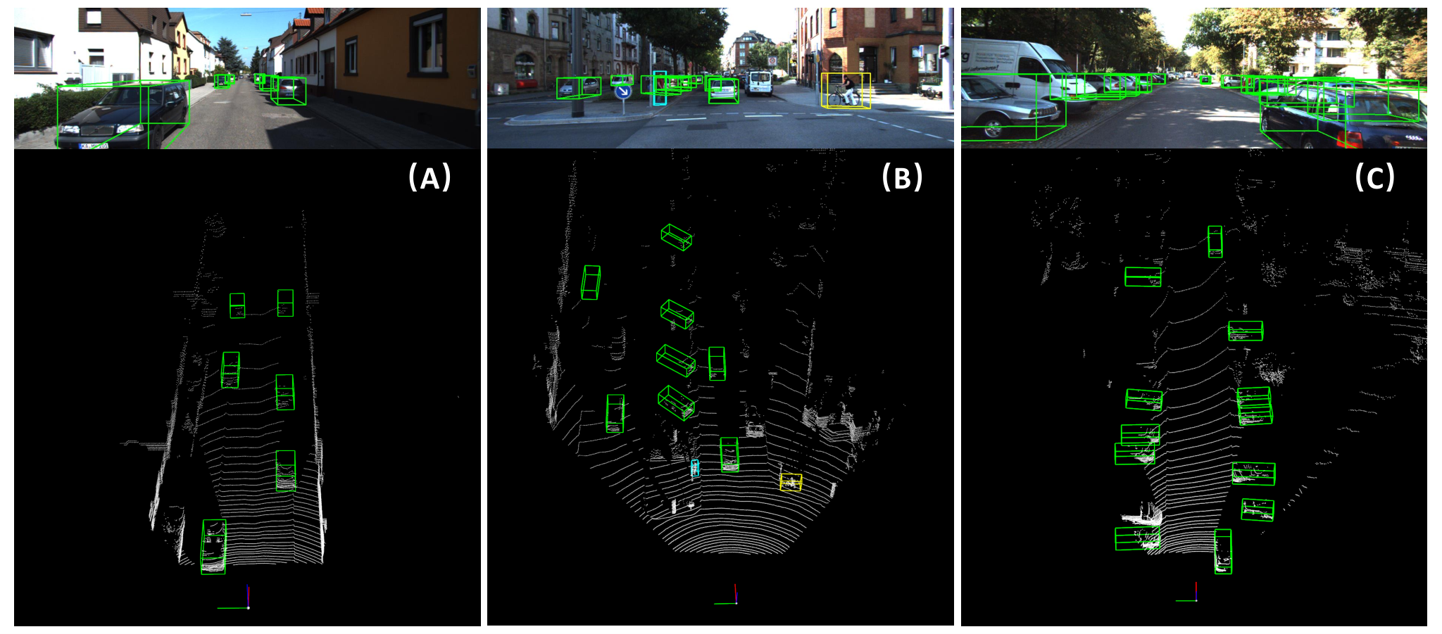
Fig. 9 shows the visualization results on the KITTI dataset. Our model performs stably and makes accurate detection in complex situations, especially in Fig. 9 (B). Moreover, as shown in Table 1, higher average precision on car and cyclist proves the effectiveness of our proposed methods. However, our method still lags behind some state-of-the-art methods for detecting small objects such as pedestrian. The reason is that our segmentation module performs badly to classify small objects, resulting in fewer keypoints on pedestrians retained to integrate valuable feature for refinement.
5 Conclusion
In this paper, we present the PV-RCNN++ framework, a novel Semantical Point-Voxel Feature Interaction for 3D object detection, which achieves 81.60, 40.18, 68.21 3D mAP on Car, Pedestrian, and Cyclist on the KITTI benchmark. We introduce a carefully designed point cloud segmentation module as guide to sample more object-related keypoints. Through fast voxel query based on Manhattan distance, we speed up the interaction between keypoints and voxels to efficiently group the neighboring voxel-wise feature. The proposed attention-based residual PointNet abstracts more fine-grained 3D information from nearby voxels, providing more comprehensive features for the succeeding refinement. Extensive experiments on KITTI dataset demonstrate that our proposed semantic-guided voxel-to-keypoint detector precisely summarizes the valuable information from pivotal areas in the point cloud and improves performance compared with previous state-of-the-art methods.
References
- Chen et al. (2022) Chen Chen, Zhe Chen, Jing Zhang, and Dacheng Tao. Sasa: Semantics-augmented set abstraction for point-based 3d object detection. arXiv e-prints, pp. arXiv–2201, 2022.
- Chen et al. (2017a) Xiaozhi Chen, Kaustav Kundu, Yukun Zhu, Huimin Ma, Sanja Fidler, and Raquel Urtasun. 3d object proposals using stereo imagery for accurate object class detection. IEEE transactions on pattern analysis and machine intelligence, 40(5):1259–1272, 2017a.
- Chen et al. (2017b) Xiaozhi Chen, Huimin Ma, Ji Wan, Bo Li, and Tian Xia. Multi-view 3d object detection network for autonomous driving. In Proceedings of the IEEE conference on Computer Vision and Pattern Recognition, pp. 1907–1915, 2017b.
- Chen et al. (2020) Yongjian Chen, Lei Tai, Kai Sun, and Mingyang Li. Monopair: Monocular 3d object detection using pairwise spatial relationships. In Proceedings of the IEEE/CVF Conference on Computer Vision and Pattern Recognition, pp. 12093–12102, 2020.
- Deng et al. (2021) Jiajun Deng, Shaoshuai Shi, Peiwei Li, Wengang Zhou, Yanyong Zhang, and Houqiang Li. Voxel r-cnn: Towards high performance voxel-based 3d object detection. In Proceedings of the AAAI Conference on Artificial Intelligence, volume 35, pp. 1201–1209, 2021.
- Dosovitskiy et al. (2020) Alexey Dosovitskiy, Lucas Beyer, Alexander Kolesnikov, Dirk Weissenborn, Xiaohua Zhai, Thomas Unterthiner, Mostafa Dehghani, Matthias Minderer, Georg Heigold, Sylvain Gelly, et al. An image is worth 16x16 words: Transformers for image recognition at scale. arXiv preprint arXiv:2010.11929, 2020.
- Geiger et al. (2012) Andreas Geiger, Philip Lenz, and Raquel Urtasun. Are we ready for autonomous driving? the kitti vision benchmark suite. In 2012 IEEE conference on computer vision and pattern recognition, pp. 3354–3361. IEEE, 2012.
- Guo et al. (2021) Meng-Hao Guo, Jun-Xiong Cai, Zheng-Ning Liu, Tai-Jiang Mu, Ralph R Martin, and Shi-Min Hu. Pct: Point cloud transformer. Computational Visual Media, 7(2):187–199, 2021.
- He et al. (2020) Chenhang He, Hui Zeng, Jianqiang Huang, Xian-Sheng Hua, and Lei Zhang. Structure aware single-stage 3d object detection from point cloud. In Proceedings of the IEEE/CVF conference on computer vision and pattern recognition, pp. 11873–11882, 2020.
- He et al. (2016) Kaiming He, Xiangyu Zhang, Shaoqing Ren, and Jian Sun. Deep residual learning for image recognition. In Proceedings of the IEEE conference on computer vision and pattern recognition, pp. 770–778, 2016.
- He et al. (2022) Qingdong He, Zhengning Wang, Hao Zeng, Yi Zeng, and Yijun Liu. Svga-net: Sparse voxel-graph attention network for 3d object detection from point clouds. In Proceedings of the AAAI Conference on Artificial Intelligence, volume 36, pp. 870–878, 2022.
- Hinton et al. (2015) Geoffrey Hinton, Oriol Vinyals, Jeff Dean, et al. Distilling the knowledge in a neural network. arXiv preprint arXiv:1503.02531, 2(7), 2015.
- Huang et al. (2020) Tengteng Huang, Zhe Liu, Xiwu Chen, and Xiang Bai. Epnet: Enhancing point features with image semantics for 3d object detection. In European Conference on Computer Vision, pp. 35–52. Springer, 2020.
- Ji et al. (2022) Chaofeng Ji, Guizhong Liu, and Dan Zhao. Stereo 3d object detection via instance depth prior guidance and adaptive spatial feature aggregation. The Visual Computer, pp. 1–12, 2022.
- Jiang et al. (2021) Tianyuan Jiang, Nan Song, Huanyu Liu, Ruihao Yin, Ye Gong, and Jian Yao. Vic-net: Voxelization information compensation network for point cloud 3d object detection. In 2021 IEEE International Conference on Robotics and Automation (ICRA), pp. 13408–13414. IEEE, 2021.
- Ku et al. (2018) Jason Ku, Melissa Mozifian, Jungwook Lee, Ali Harakeh, and Steven L Waslander. Joint 3d proposal generation and object detection from view aggregation. In 2018 IEEE/RSJ International Conference on Intelligent Robots and Systems (IROS), pp. 1–8. IEEE, 2018.
- Lang et al. (2019) Alex H Lang, Sourabh Vora, Holger Caesar, Lubing Zhou, Jiong Yang, and Oscar Beijbom. Pointpillars: Fast encoders for object detection from point clouds. In Proceedings of the IEEE/CVF conference on computer vision and pattern recognition, pp. 12697–12705, 2019.
- Li et al. (2019a) Buyu Li, Wanli Ouyang, Lu Sheng, Xingyu Zeng, and Xiaogang Wang. Gs3d: An efficient 3d object detection framework for autonomous driving. In Proceedings of the IEEE/CVF Conference on Computer Vision and Pattern Recognition, pp. 1019–1028, 2019a.
- Li et al. (2019b) Peiliang Li, Xiaozhi Chen, and Shaojie Shen. Stereo r-cnn based 3d object detection for autonomous driving. In Proceedings of the IEEE/CVF Conference on Computer Vision and Pattern Recognition, pp. 7644–7652, 2019b.
- Li & Chen (2022) Peng Li and Yuantao Chen. Research into an image inpainting algorithm via multilevel attention progression mechanism. Mathematical Problems in Engineering, 2022:1–12, 2022.
- Lin et al. (2017) Tsung-Yi Lin, Priya Goyal, Ross Girshick, Kaiming He, and Piotr Dollár. Focal loss for dense object detection. In Proceedings of the IEEE international conference on computer vision, pp. 2980–2988, 2017.
- Luo et al. (2021) Chenxu Luo, Xiaodong Yang, and Alan Yuille. Exploring simple 3d multi-object tracking for autonomous driving. In Proceedings of the IEEE/CVF International Conference on Computer Vision, pp. 10488–10497, 2021.
- Ma et al. (2022) Xu Ma, Can Qin, Haoxuan You, Haoxi Ran, and Yun Fu. Rethinking network design and local geometry in point cloud: A simple residual mlp framework. arXiv preprint arXiv:2202.07123, 2022.
- Noh et al. (2021) Jongyoun Noh, Sanghoon Lee, and Bumsub Ham. Hvpr: Hybrid voxel-point representation for single-stage 3d object detection. In Proceedings of the IEEE/CVF Conference on Computer Vision and Pattern Recognition (CVPR), pp. 14605–14614, June 2021.
- Pang et al. (2022) Su Pang, Daniel Morris, and Hayder Radha. Fast-clocs: Fast camera-lidar object candidates fusion for 3d object detection. In Proceedings of the IEEE/CVF Winter Conference on Applications of Computer Vision, pp. 187–196, 2022.
- Qi et al. (2017) Charles R Qi, Li Yi, Hao Su, and Leonidas J Guibas. Pointnet++ deep hierarchical feature learning on point sets in a metric space. In Proceedings of the 31st International Conference on Neural Information Processing Systems, pp. 5105–5114, 2017.
- Qi et al. (2018) Charles R Qi, Wei Liu, Chenxia Wu, Hao Su, and Leonidas J Guibas. Frustum pointnets for 3d object detection from rgb-d data. In Proceedings of the IEEE conference on computer vision and pattern recognition, pp. 918–927, 2018.
- Reading et al. (2021) Cody Reading, Ali Harakeh, Julia Chae, and Steven L Waslander. Categorical depth distribution network for monocular 3d object detection. In Proceedings of the IEEE/CVF Conference on Computer Vision and Pattern Recognition, pp. 8555–8564, 2021.
- Ren et al. (2016) S Ren, K He, R Girshick, and J Sun. Faster r-cnn: Towards real-time object detection with region proposal networks. IEEE Transactions on Pattern Analysis and Machine Intelligence, 39(6):1137–1149, 2016.
- Scarselli et al. (2008) Franco Scarselli, Marco Gori, Ah Chung Tsoi, Markus Hagenbuchner, and Gabriele Monfardini. The graph neural network model. IEEE transactions on neural networks, 20(1):61–80, 2008.
- Shi et al. (2019a) Shaoshuai Shi, Xiaogang Wang, and Hongsheng Li. Pointrcnn: 3d object proposal generation and detection from point cloud. In Proceedings of the IEEE/CVF conference on computer vision and pattern recognition, pp. 770–779, 2019a.
- Shi et al. (2019b) Shaoshuai Shi, Zhe Wang, Xiaogang Wang, and Hongsheng Li. Part-aˆ 2 net: 3d part-aware and aggregation neural network for object detection from point cloud. arXiv preprint arXiv:1907.03670, 2(3), 2019b.
- Shi et al. (2020) Shaoshuai Shi, Chaoxu Guo, Li Jiang, Zhe Wang, Jianping Shi, Xiaogang Wang, and Hongsheng Li. Pv-rcnn: Point-voxel feature set abstraction for 3d object detection. In Proceedings of the IEEE/CVF Conference on Computer Vision and Pattern Recognition, pp. 10529–10538, 2020.
- Shi & Rajkumar (2020) Weijing Shi and Raj Rajkumar. Point-gnn: Graph neural network for 3d object detection in a point cloud. In Proceedings of the IEEE/CVF conference on computer vision and pattern recognition, pp. 1711–1719, 2020.
- Shu et al. (2021) Xiangbo Shu, Liyan Zhang, Guo-Jun Qi, Wei Liu, and Jinhui Tang. Spatiotemporal co-attention recurrent neural networks for human-skeleton motion prediction. IEEE Transactions on Pattern Analysis and Machine Intelligence, 44(6):3300–3315, 2021.
- Shu et al. (2022) Xiangbo Shu, Jiawen Yang, Rui Yan, and Yan Song. Expansion-squeeze-excitation fusion network for elderly activity recognition. IEEE Transactions on Circuits and Systems for Video Technology, pp. 1–1, 2022.
- Tang et al. (2022) Jinhui Tang, Xiangbo Shu, Rui Yan, and Liyan Zhang. Coherence constrained graph lstm for group activity recognition. IEEE transactions on pattern analysis and machine intelligence, 44(2):636–647, 2022.
- Team (2020) OpenPCDet Development Team. Openpcdet: An open-source toolbox for 3d object detection from point clouds. https://github.com/open-mmlab/OpenPCDet, 2020.
- Vaswani et al. (2017) Ashish Vaswani, Noam Shazeer, Niki Parmar, Jakob Uszkoreit, Llion Jones, Aidan N Gomez, Lukasz Kaiser, and Illia Polosukhin. Attention is all you need. arXiv e-prints, pp. arXiv–1706, 2017.
- Vora et al. (2020) Sourabh Vora, Alex H Lang, Bassam Helou, and Oscar Beijbom. Pointpainting: Sequential fusion for 3d object detection. In Proceedings of the IEEE/CVF conference on computer vision and pattern recognition, pp. 4604–4612, 2020.
- Wang et al. (2022a) Zhoutao Wang, Qian Xie, Mingqiang Wei, Kun Long, and Jun Wang. Multi-feature fusion votenet for 3d object detection. ACM Trans. Multim. Comput. Commun. Appl., 18(1):6:1–6:17, 2022a.
- Wang et al. (2022b) Zhoutao Wang, Qian Xie, Mingqiang Wei, Kun Long, and Jun Wang. Multi-feature fusion votenet for 3d object detection. ACM Transactions on Multimedia Computing, Communications, and Applications (TOMM), 18(1):1–17, 2022b.
- Wei et al. (2022) Zongqi Wei, Dong Liang, Dong Zhang, Liyan Zhang, Qixiang Geng, Mingqiang Wei, and Huiyu Zhou. Learning calibrated-guidance for object detection in aerial images. IEEE J. Sel. Top. Appl. Earth Obs. Remote. Sens., 15:2721–2733, 2022.
- Xie et al. (2021) Qian Xie, Yu-Kun Lai, Jing Wu, Zhoutao Wang, Dening Lu, Mingqiang Wei, and Jun Wang. Venet: Voting enhancement network for 3d object detection. In Proceedings of the IEEE/CVF International Conference on Computer Vision, pp. 3712–3721, 2021.
- Yan & Salman (2017) Chen Yan and Emre Salman. Mono3d: Open source cell library for monolithic 3-d integrated circuits. IEEE Transactions on Circuits and Systems I: Regular Papers, 65(3):1075–1085, 2017.
- Yan et al. (2018) Yan Yan, Yuxing Mao, and Bo Li. Second: Sparsely embedded convolutional detection. Sensors, 18(10):3337, 2018.
- Yang et al. (2019) Zetong Yang, Yanan Sun, Shu Liu, Xiaoyong Shen, and Jiaya Jia. Std: Sparse-to-dense 3d object detector for point cloud. In Proceedings of the IEEE/CVF international conference on computer vision, pp. 1951–1960, 2019.
- Yang et al. (2020) Zetong Yang, Yanan Sun, Shu Liu, and Jiaya Jia. 3dssd: Point-based 3d single stage object detector. In Proceedings of the IEEE/CVF conference on computer vision and pattern recognition, pp. 11040–11048, 2020.
- Ye et al. (2020) Maosheng Ye, Shuangjie Xu, and Tongyi Cao. Hvnet: Hybrid voxel network for lidar based 3d object detection. In Proceedings of the IEEE/CVF conference on computer vision and pattern recognition, pp. 1631–1640, 2020.
- Yin et al. (2021) Tianwei Yin, Xingyi Zhou, and Philipp Krahenbuhl. Center-based 3d object detection and tracking. In Proceedings of the IEEE/CVF conference on computer vision and pattern recognition, pp. 11784–11793, 2021.
- Yoo et al. (2020) Jin Hyeok Yoo, Yecheol Kim, Jisong Kim, and Jun Won Choi. 3d-cvf: Generating joint camera and lidar features using cross-view spatial feature fusion for 3d object detection. In European Conference on Computer Vision, pp. 720–736. Springer, 2020.
- Yuan et al. (2018) Wentao Yuan, Tejas Khot, David Held, Christoph Mertz, and Martial Hebert. Pcn: Point completion network. In 2018 International Conference on 3D Vision (3DV), pp. 728–737. IEEE, 2018.
- Zarzar et al. (2019) Jesus Zarzar, Silvio Giancola, and Bernard Ghanem. Pointrgcn: Graph convolution networks for 3d vehicles detection refinement. arXiv preprint arXiv:1911.12236, 2019.
- Zhang et al. (2021) Yanan Zhang, Di Huang, and Yunhong Wang. Pc-rgnn: Point cloud completion and graph neural network for 3d object detection. In Proceedings of the AAAI Conference on Artificial Intelligence, volume 35, pp. 3430–3437, 2021.
- Zhang et al. (2022a) Yanan Zhang, Jiaxin Chen, and Di Huang. Cat-det: Contrastively augmented transformer for multi-modal 3d object detection. In Proceedings of the IEEE/CVF Conference on Computer Vision and Pattern Recognition (CVPR), pp. 908–917, June 2022a.
- Zhang et al. (2022b) Yifan Zhang, Qingyong Hu, Guoquan Xu, Yanxin Ma, Jianwei Wan, and Yulan Guo. Not all points are equal: Learning highly efficient point-based detectors for 3d lidar point clouds. In Proceedings of the IEEE/CVF Conference on Computer Vision and Pattern Recognition, pp. 18953–18962, 2022b.
- Zhao et al. (2021) Hengshuang Zhao, Li Jiang, Jiaya Jia, Philip HS Torr, and Vladlen Koltun. Point transformer. In Proceedings of the IEEE/CVF International Conference on Computer Vision, pp. 16259–16268, 2021.
- Zheng et al. (2022) Chengyu Zheng, Ding Shi, Xuefeng Yan, Dong Liang, Mingqiang Wei, Xin Yang, Yanwen Guo, and Haoran Xie. Glassnet: Label decoupling-based three-stream neural network for robust image glass detection. Comput. Graph. Forum, 41(1):377–388, 2022.
- Zheng et al. (2021a) Wu Zheng, Weiliang Tang, Sijin Chen, Li Jiang, and Chi-Wing Fu. Cia-ssd: Confident iou-aware single-stage object detector from point cloud. In Proceedings of the AAAI conference on artificial intelligence, volume 35, pp. 3555–3562, 2021a.
- Zheng et al. (2021b) Wu Zheng, Weiliang Tang, Li Jiang, and Chi-Wing Fu. Se-ssd: Self-ensembling single-stage object detector from point cloud. In Proceedings of the IEEE/CVF Conference on Computer Vision and Pattern Recognition, pp. 14494–14503, 2021b.
- Zhou & Tuzel (2018) Yin Zhou and Oncel Tuzel. Voxelnet: End-to-end learning for point cloud based 3d object detection. In Proceedings of the IEEE conference on computer vision and pattern recognition, pp. 4490–4499, 2018.