跳到论文正文
W Papers独立论文阅读器 arXiv:2208.13167 论文正文 计算阅读时间 · 0%
引用这篇论文根据当前论文元数据生成,正式投稿前建议核对。


License: CC BY 4.0
arXiv:2208.13167v2 [math.DS] 11 Jul 2023

Large amplitude radially symmetric spots and gaps in a dryland ecosystem model

Eleanor Byrnes Thanks: Department of Applied Mathematics, University of Washington, Seattle, WA, USA    Paul Carter Thanks: Department of Mathematics, University of California, Irvine, CA, USA    Arjen Doelman Thanks: Mathematisch Instituut, Universiteit Leiden, Leiden, NL    Lily Liu Thanks: University of Chicago, Chicago, IL, USA
Abstract

We construct far-from-onset radially symmetric spot and gap solutions in a two-component dryland ecosystem model of vegetation pattern formation on flat terrain, using spatial dynamics and geometric singular perturbation theory. We draw connections between the geometry of the spot and gap solutions with that of traveling and stationary front solutions in the same model. In particular, we demonstrate the instability of spots of large radius by deriving an asymptotic relationship between a critical eigenvalue associated with the spot and a coefficient which encodes the sideband instability of a nearby stationary front. Furthermore, we demonstrate that spots are unstable to a range of perturbations of intermediate wavelength in the angular direction, provided the spot radius is not too small. Our results are accompanied by numerical simulations and spectral computations.

1 Introduction

The phenomenon of vegetation pattern formation in dryland ecosystems has attracted attention in the last several decades as a mechanism of ecological resilience. While frequently considered to be an early warning sign for desertification [16, 17, 26, 28, 32, 33, 34], the formation of localized vegetation patches or patterns has also been viewed as a means of evading such critical transitions [30]. The interaction of infiltration feedback mechanisms and competition for water resources results in the formation of vegetation patches [25, 31, 37, 43, 45]. On sloped terrain, one observes vegetation stripes, or bands, aligned perpendicular to the slope, while on flat ground spots, gaps, or disorganized labyrinth patterns are prevalent [1, 6, 7, 13, 24, 40]. Spots, gaps, rings or other radially symmetric patterns (sometimes called “fairy circles”) have been observed extensively in drylands in Australia and Africa [14, 27, 29] (and other ecosystems, such as submarine seascapes [35]), and have served as the focus of many studies of self-organization in ecosystems.

Vegetation pattern formation is frequently modeled by multi-component reaction diffusion systems. In such models, there is a well-developed theory of spot and stripe pattern formation near the onset of Turing instabilities [17, 15, 39]. However, far less is known analytically concerning large amplitude or far-from-onset planar vegetation patterns. A number of studies have considered existence and stability properties of banded vegetation [2, 3, 10, 38], as well as desertification fronts [4, 12], but less is known concerning far-from-onset radially symmetric vegetation patches. Prior work has considered small amplitude radial solutions [18] and 1\displaystyle 1D simplifications [19]. However, to our knowledge, no rigorous studies exist concerning large amplitude radially symmetric vegetation patches in a dryland ecosystem model.

We consider the model introduced in [2]

Ut=Δ​U+a−U−U​V2Vt=δ2​Δ​V−m​V+U​V2​(1−b​V),\displaystyle\displaystyle\begin{split}U_{t}&=\Delta U+a-U-UV^{2}\\ V_{t}&=\delta^{2}\Delta V-mV+UV^{2}(1-bV),\end{split} (1.1)

which is a modification of the dryland ecosystem model originally proposed by Klausmeier [20]. This model also coincides with that studied in [11], in the case of a single species. Here U\displaystyle U represents water availability, V\displaystyle V represents vegetation density, and the parameters a,m,b\displaystyle a,m,b are positive and represent rainfall, mortality, and inverse of soil carrying capacity, respectively. The diffusion coefficient δ2\displaystyle\delta^{2} represents the ratio of timescales of diffusion of water vs. vegetation. Here, we assume that water diffuses much faster than vegetation, so that 0<δ≪1\displaystyle 0<\delta\ll 1 is a small parameter [33]. We note that Klausmeier’s model originally had b=0\displaystyle b=0. While a singular perturbation analysis of this case is possible (see, e.g. [3]), this limit is highly singular, requiring several rescalings and blow up techniques to account for passage near a non-hyperbolic slow manifold. Here, we therefore focus on the case b>0\displaystyle b>0.

We are interested in the formation of radially symmetric vegetation spots (localized vegetation patches surrounded by bare soil) and gaps (localized regions of bare soil in an otherwise uniformly vegetated state) in (1.1). Exploiting the small parameter δ≪1\displaystyle\delta\ll 1, we will use geometric singular perturbation methods to construct radially symmetric solutions through a spatial dynamics approach in the radial coordinate. Our approach is similar to that in [41], in which the authors construct far-from-onset spot solutions in a 3-component FitzHugh–Nagumo model. However, the nonlinearities in (1.1) introduce complications in the analysis due to the fact that the reduced flow on the resulting slow manifolds is no longer linear as in the case in [41]. However, we will show that radial solutions can still be constructed in (1.1).

Remark 1.1.

In the setting of classical models like Gray-Scott, Gierer-Meinhardt and Schnakenberg, the existence, stability and interactions of radially symmetric localized ‘spikes’ has been studied – see for instance  [5, 23, 44] and the references therein. However, these patterns differ from the ones considered here since they have a homoclinic nature: unlike the present gaps and spots, the regions in which these spikes are not close to the background states are asymptotically small. The patterns considered here can be seen as two-dimensional (radially symmetric) versions of the one-dimensional ‘mesa patterns’ studied in [22] and in  [19] in the setting of vegetation patterns. Like in the present model, and unlike in [41, 42], the ‘slow flows’ (for the spatial dynamics) considered in these papers are nonlinear – which is typically the case for ecosystem models [9].

The system (1.1) admits (up to) three homogeneous steady states: the desert state (U,V)=(U0,V0):=(a,0)\displaystyle(U,V)=(U_{0},V_{0}):=(a,0) and if am>2​(b+1+b2)\displaystyle\frac{a}{m}>2(b+\sqrt{1+b^{2}}), there are two additional vegetated steady states (U,V)=(U1,2,V1,2)\displaystyle(U,V)=(U_{1,2},V_{1,2}) where

U1,2\displaystyle\displaystyle U_{1,2} =m⁡(am−V1,21−b​V1,2),V1,2=am∓(am)2−4​(1+am​b)2​(1+am​b)\displaystyle\displaystyle=m\left(\frac{a}{m}-\frac{V_{1,2}}{1-bV_{1,2}}\right),\qquad V_{1,2}=\frac{\frac{a}{m}\mp\sqrt{\left(\frac{a}{m}\right)^{2}-4\left(1+\frac{a}{m}b\right)}}{2\left(1+\frac{a}{m}b\right)} (1.2)

which coincide at the critical value am=2​(b+1+b2)\displaystyle\frac{a}{m}=2(b+\sqrt{1+b^{2}}).

We search for stationary solutions, which are radially symmetric, so that (U,V)​(x,y,t)=(u,v)​(r),r∈[0,∞)\displaystyle(U,V)(x,y,t)=(u,v)(r),r\in[0,\infty), and Δ=∂r2+r−1∂r\displaystyle\Delta=\partial_{r}^{2}+r^{-1}\partial_{r} under planar radial symmetry, where r=(x2+y2)1/2\displaystyle r=(x^{2}+y^{2})^{1/2}. Such solutions satisfy the ordinary differential equation

0=ur​r+1r​ur+a−u−u​v20=δ2​(vr​r+1r​vr)−m​v+u​v2​(1−b​v),\displaystyle\displaystyle\begin{split}0&=u_{rr}+\frac{1}{r}u_{r}+a-u-uv^{2}\\ 0&=\delta^{2}\left(v_{rr}+\frac{1}{r}v_{r}\right)-mv+uv^{2}(1-bv),\end{split} (1.3)

which can be rewritten as a first order non-autonomous system

ur=ppr=−pr−a+u+u​v2δ​vr=qδ​qr=−δ​qr+m​v−u​v2​(1−b​v),\displaystyle\displaystyle\begin{split}u_{r}&=p\\ p_{r}&=-\frac{p}{r}-a+u+uv^{2}\\ \delta v_{r}&=q\\ \delta q_{r}&=-\frac{\delta q}{r}+mv-uv^{2}(1-bv),\end{split} (1.4)

This system admits up to three equilibria given by the steady states above: the desert state P0=(a,0,0,0)\displaystyle P_{0}=(a,0,0,0), and if am>2​(b+1+b2)\displaystyle\frac{a}{m}>2(b+\sqrt{1+b^{2}}), there are two additional equilibria P1,2:=(U1,2,0,V1,2,0)\displaystyle P_{1,2}:=(U_{1,2},0,V_{1,2},0) corresponding to uniform vegetation.

Spots, gaps, and other localized radially symmetric solutions are constructed as orbits of (1.4) which are asymptotic as r→∞\displaystyle r\to\infty to one of these steady states, and which are bounded as r→0\displaystyle r\to 0. In order to find solutions of this system, we construct candidate solution orbits in different subsets of the spatial domain r∈[0,∞)\displaystyle r\in[0,\infty) and glue these together to build a solution on the entire domain. In particular, we construct the solution over three primary regions: the core r∈[0,rc]\displaystyle r\in[0,r_{\mathrm{c}}], where rc=𝒪⁡(δ)\displaystyle r_{\mathrm{c}}=\mathcal{O}(\delta), the far field r∈[rI,∞)\displaystyle r\in[r_{I},\infty), where rI=𝒪⁡(1)\displaystyle r_{I}=\mathcal{O}(1), and the transition region(s) in between; see Figure 1.

Figure 1: Shown is a schematic of a radial profile for a vegetation spot solution (left) and gap solution (right) of (1.3) as in Theorem 1.2 and 1.3, respectively. The profile contains a sharp transition from the vegetated state to the bare soil state in an interval of width 𝒪⁡(δ)\displaystyle\mathcal{O}(\delta) of the critical radius rI=𝒪⁡(1)\displaystyle r_{I}=\mathcal{O}(1).

Our main result concerning the existence of spots is the following.

Theorem 1.2.

(Existence of spots) Fix a,m,b>0\displaystyle a,m,b>0 satisfying

max⁡{9​b2,4​b+1b}<am<9​b2+2b.\displaystyle\displaystyle\max\left\{\frac{9b}{2},4b+\frac{1}{b}\right\}<\frac{a}{m}<\frac{9b}{2}+\frac{2}{b}. (1.5)

Suppose

∫U29​b​m2u−2​m​b+u2−4​u​m​b2​b2​𝑑u\displaystyle\displaystyle\int_{U_{2}}^{\frac{9bm}{2}}\frac{u-2mb+\sqrt{u^{2}-4umb}}{2b^{2}}\mathrm{d}u >12​(a−U2)2,\displaystyle\displaystyle>\frac{1}{2}(a-U_{2})^{2}, (1.6)

or equivalently,

32−log⁡(2)+U22​m2​(a−U2)+log⁡(bm​(a−U2))−bm​(a−U2)>2​b2+12​m2​(a−U2)2\displaystyle\displaystyle\frac{3}{2}-\log(2)+\frac{U_{2}}{2m^{2}}\left(a-U_{2}\right)+\log\left(\frac{b}{m}\left(a-U_{2}\right)\right)-\frac{b}{m}\left(a-U_{2}\right)>\frac{2b^{2}+1}{2m^{2}}\left(a-U_{2}\right)^{2} (1.7)

where U2\displaystyle U_{2} is defined as in (1.2). Then there exists Vc​(a,b,m)>0\displaystyle V_{\mathrm{c}}(a,b,m)>0 and rI​(a,b,m)>0\displaystyle r_{I}(a,b,m)>0 such that for all sufficiently small δ>0\displaystyle\delta>0, (1.1) admits a stationary, bounded, radially symmetric vegetation spot solution (U,V)=(usp,vsp)​(r,a,b,m,δ)\displaystyle(U,V)=(u_{\mathrm{sp}},v_{\mathrm{sp}})(r;a,b,m,\delta) satisfying

limr→0vsp​(r,a,b,m,δ)\displaystyle\displaystyle\lim_{r\to 0}v_{\mathrm{sp}}(r;a,b,m,\delta) =Vc​(a,b,m)+𝒪⁡(δ),limr→∞vsp​(r,a,b,m,δ)=0\displaystyle\displaystyle=V_{\mathrm{c}}(a,b,m)+\mathcal{O}(\delta),\qquad\lim_{r\to\infty}v_{\mathrm{sp}}(r;a,b,m,\delta)=0

with a single interface between the vegetated and desert states occurring at the radius r=rI​(a,b,m)+𝒪⁡(δ)\displaystyle r=r_{I}(a,b,m)+\mathcal{O}(\delta).

Similarly, we have the following theorem concerning the existence of gaps.

Theorem 1.3.

(Existence of gaps) Fix a,m,b>0\displaystyle a,m,b>0 satisfying (1.5). Suppose

∫U29​b​m2u−2​m​b+u2−4​u​m​b2​b2​𝑑u<12​(a−U2)2\displaystyle\displaystyle\int_{U_{2}}^{\frac{9bm}{2}}\frac{u-2mb+\sqrt{u^{2}-4umb}}{2b^{2}}\mathrm{d}u<\frac{1}{2}(a-U_{2})^{2} (1.8)

or equivalently,

32−log⁡(2)+U22​m2​(a−U2)+log⁡(bm​(a−U2))−bm​(a−U2)<2​b2+12​m2​(a−U2)2\displaystyle\displaystyle\frac{3}{2}-\log(2)+\frac{U_{2}}{2m^{2}}\left(a-U_{2}\right)+\log\left(\frac{b}{m}\left(a-U_{2}\right)\right)-\frac{b}{m}\left(a-U_{2}\right)<\frac{2b^{2}+1}{2m^{2}}\left(a-U_{2}\right)^{2} (1.9)

where U2\displaystyle U_{2} is defined as in (1.2). Then there exists rI​(a,b,m)>0\displaystyle r_{I}(a,b,m)>0 and ν>0\displaystyle\nu>0 such that for all sufficiently small δ>0\displaystyle\delta>0, (1.1) admits a stationary, bounded, radially symmetric vegetation gap solution (U,V)=(ug,vg)​(r,a,b,m,δ)\displaystyle(U,V)=(u_{\mathrm{g}},v_{\mathrm{g}})(r;a,b,m,\delta) satisfying

limr→0vg​(r,a,b,m,δ)\displaystyle\displaystyle\lim_{r\to 0}v_{\mathrm{g}}(r;a,b,m,\delta) =𝒪(e−ν/δ),limr→∞vg(r;a,b,m,δ)=V2+𝒪(δ),\displaystyle\displaystyle=\mathcal{O}(e^{-\nu/\delta}),\qquad\lim_{r\to\infty}v_{\mathrm{g}}(r;a,b,m,\delta)=V_{2}+\mathcal{O}(\delta),

where V2\displaystyle V_{2} is defined as in (1.2), with a single interface between the vegetated and desert states occurring at the radius r=rI​(a,b,m)+𝒪⁡(δ)\displaystyle r=r_{I}(a,b,m)+\mathcal{O}(\delta).

See Figure 2 for a visualization of the condition (1.5) necessary for the existence of spots/gaps in Theorems 1.2–1.3.

Figure 2: Plotted are the curves am=9​b2\displaystyle\frac{a}{m}=\frac{9b}{2} (black), am=4​b+1b\displaystyle\frac{a}{m}=4b+\frac{1}{b} (dotted red), and am=9​b2+2b\displaystyle\frac{a}{m}=\frac{9b}{2}+\frac{2}{b} (dashed blue). The shaded region corresponds to the region in parameter space where the condition (1.5) is satisfied.
Remark 1.4.

The methods used in this paper to construct radially symmetric spot and gap solutions can be applied in a similar manner for the construction of solutions such as rings, targets, or other radially symmetric profiles, with different, perhaps more complex, conditions on parameters which ensure their existence. We provide some numerical evidence for the existence of such solutions in §5 and describe how one might go about constructing these orbits, but do not provide the lengthy technical details here.

The spot and gap solutions of Theorems 1.2–1.3 will be constructed as heteroclinic orbits for r∈[0,∞)\displaystyle r\in[0,\infty) using geometric singular perturbation theory. The main idea, following [41], is to find the orbits as intersections of a core manifold of solutions which remain bounded at r→0\displaystyle r\to 0, and a far-field manifold of solutions which decay to one of the states P0\displaystyle P_{0} or P2\displaystyle P_{2} as r→∞\displaystyle r\to\infty. These manifolds are each three-dimensional, and, unlike in [41], it is not possible to obtain an explicit description of these manifolds due to the fact that the flow on (one of) the slow manifolds of (1.4) is nonlinear. This introduces complications which are handled through the use of an intermediate scaling and careful qualitative analysis of the nonlinear non-autonomous reduced flow on this slow manifold. The non-autonomous nature of the equation (1.4) makes this a somewhat challenging construction. To demonstrate how these orbits are constructed using the slow/fast geometry of (1.4), it is helpful to first consider the simpler construction of traveling or stationary planar front solutions of (1.1), which manifest as heteroclinic orbits in an appropriate traveling equation with a similar geometry to that of (1.4).

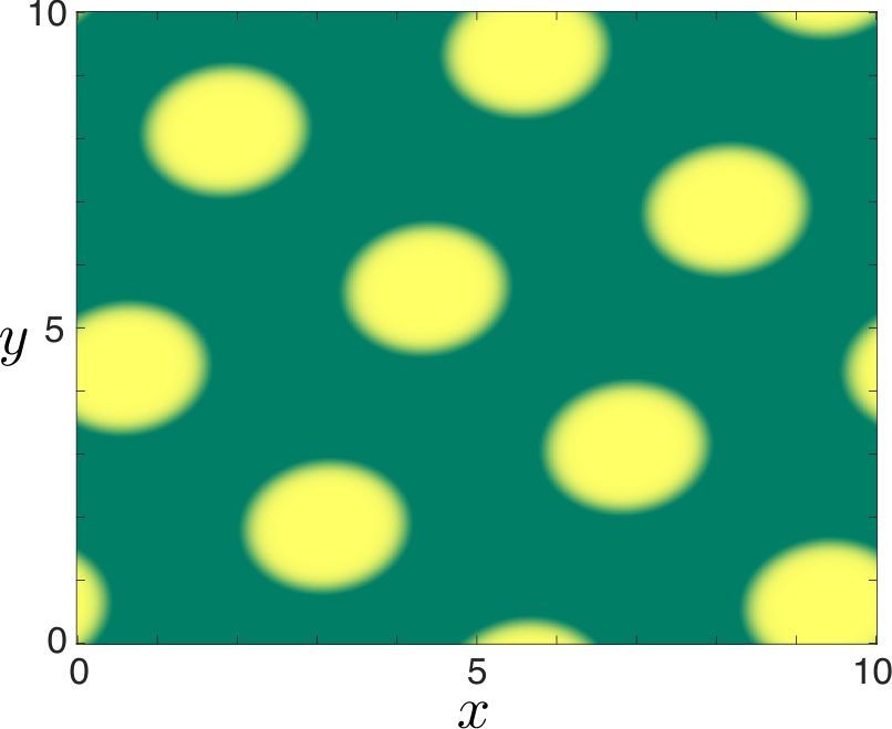
It is shown in companion paper [4] that the invasion fronts in (1.1) – that can be seen as spots or gaps with radius rI→∞\displaystyle r_{I}\to\infty – are unstable with respect to a sideband/finger instability. Therefore, we next consider the stability of spots. Without going into the details of a fully rigorous analysis, we first consider the spectral stability problem for large spots. By a careful asymptotic analysis we recover the sideband instability mechanism and conclude that large spots are unstable and will typically form finger-like patterns – like the planar invasion fronts. By similarity, we conclude that the same is true for large gaps. These observations are confirmed by direct simulations: in Fig. 9 in §5 we show snapshots of a spot and a gap that both evolve towards labyrinthine patterns after undergoing such an instability. Moreover, we subsequently conclude by considering perturbations within a range of intermediate wave numbers that spots (and gaps) with 𝒪⁡(1)\displaystyle\mathcal{O}(1) radius rI\displaystyle r_{I} must also be unstable: only sufficiently small spots and gaps may possibly be stable – see again §5 and especially Fig. 10 for a brief numerical study. These small gaps correspond to fairy circles [14] and also appear as stable vegetation patterns in numerical simulations of the dryland ecosystem model of [46] – a model that can be seen as a slightly more extended version of (1.1) [4] (and that has been deduced from more extended models to study fairy circles).

The set-up of the paper is as follows. In §2, we consider the construction of traveling fronts in (1.1), while in §3, we treat the radially symmetric case and provide the proofs of Theorems 1.2–1.3. The spectral stability of the radial spot and gap solutions is considered in §4 using formal asymptotic methods, and we include numerical simulations and a brief discussion in §5.

2 Stationary and traveling planar fronts

To motivate the approach for the existence analysis of radially symmetric solutions of (1.1), we first consider the (simpler) case of constructing stationary and traveling front solutions. We pose the traveling wave ansatz (u,v)​(x,y,t)=(u,v)​(ξ)\displaystyle(u,v)(x,y,t)=(u,v)(\xi), where ξ=x−δ​c​t\displaystyle\xi=x-\delta ct is a traveling wave coordinate; here c=0\displaystyle c=0 corresponds to stationary front solutions, while c≠0\displaystyle c\neq 0 corresponds to solutions which propagate with wave speed δ​c\displaystyle\delta c.

Using a geometric singular perturbation approach, we can construct bistable front solutions as perturbations from slow/fast heteroclinic orbits between the desert state (U,V)=(a,0)\displaystyle(U,V)=(a,0) and the vegetated state (U,V)=(U2,V2)\displaystyle(U,V)=(U_{2},V_{2}) in the traveling wave ODE

0=uξ​ξ+δ​c​uξ+a−u−u​v20=δ2​vξ​ξ+δ​c​vξ−m​v+u​v2​(1−b​v).\displaystyle\displaystyle\begin{split}0&=u_{\xi\xi}+\delta cu_{\xi}+a-u-uv^{2}\\ 0&=\delta^{2}v_{\xi\xi}+\delta cv_{\xi}-mv+uv^{2}(1-bv).\end{split} (2.1)

We note that in the case c=0\displaystyle c=0, the system (2.1) corresponds to (1.3) in the far field limit r→∞\displaystyle r\to\infty. Thus, it is natural to first consider the geometry of (2.1), as solutions with radial symmetry are constructed by matching a solution which is bounded near the core r=0\displaystyle r=0, with a stationary solution which (approximately) satisfies (2.1) in the far field limit r→∞\displaystyle r\to\infty.

2.1 Slow/fast analysis

We can write (2.1) as a first order system

uξ=ppξ=−δ​c​p−a+u+u​v2δ​vξ=qδ​qξ=−c​q+m​v−u​v2​(1−b​v),\displaystyle\displaystyle\begin{split}u_{\xi}&=p\\ p_{\xi}&=-\delta cp-a+u+uv^{2}\\ \delta v_{\xi}&=q\\ \delta q_{\xi}&=-cq+mv-uv^{2}(1-bv),\end{split} (2.2)

which we refer to as the slow system, and upon rescaling ξ=δ​ζ\displaystyle\xi=\delta\zeta, we obtain the equivalent fast system

uζ=δ​ppζ=δ⁡(−δ​c​p−a+u+u​v2)vζ=qqζ=−c​q+m​v−u​v2​(1−b​v),\displaystyle\displaystyle\begin{split}u_{\zeta}&=\delta p\\ p_{\zeta}&=\delta\left(-\delta cp-a+u+uv^{2}\right)\\ v_{\zeta}&=q\\ q_{\zeta}&=-cq+mv-uv^{2}(1-bv),\end{split} (2.3)

Setting δ=0\displaystyle\delta=0 in (2.3) yields the layer problem

vζ=qqζ=−c​q+m​v−u​v2​(1−b​v).\displaystyle\displaystyle\begin{split}v_{\zeta}&=q\\ q_{\zeta}&=-cq+mv-uv^{2}(1-bv).\end{split} (2.4)

This system admits up to three equilibria depending on u\displaystyle u, given by M0​(u):=(0,0)\displaystyle M_{0}(u):=(0,0), and if u>4​b​m\displaystyle u>4bm, M±​(u):=(v±​(u),0)\displaystyle M_{\pm}(u):=(v_{\pm}(u),0), where

v±​(u):=1±1−4​b​mu2​b.\displaystyle\displaystyle v_{\pm}(u):=\frac{1\pm\sqrt{1-\frac{4bm}{u}}}{2b}. (2.5)

When u=4​b​m\displaystyle u=4bm, the two equilibria M+​(4​b​m)=M−​(4​b​m)\displaystyle M_{+}(4bm)=M_{-}(4bm) coincide. Computing the linearization

Jlayer=(01m−2​u​v+3​b​u​v2−c),\displaystyle\displaystyle J_{\mathrm{layer}}=\begin{pmatrix}0&1\\ m-2uv+3buv^{2}&-c\end{pmatrix}, (2.6)

a short computation shows that for m,b>0\displaystyle m,b>0 the fixed points M0\displaystyle M_{0} and M+​(u),u>4​b​m\displaystyle M_{+}(u),u>4bm are always of saddle type, while M−​(u)\displaystyle M_{-}(u) is focus or node for c≠0\displaystyle c\neq 0, and a center for c=0\displaystyle c=0. The equilibrium M+​(4​b​m)=M−​(4​b​m)\displaystyle M_{+}(4bm)=M_{-}(4bm) is nonhyperbolic. Taken together, the set of equilibria of the layer equation (2.4) corresponds to the critical manifold

ℳ0={(u,p,v,q)∈ℝ4:q=0,mv=uv2(1−bv)},\displaystyle\displaystyle\mathcal{M}_{0}=\left\{(u,p,v,q)\in\mathbb{R}^{4}:q=0,mv=uv^{2}(1-bv)\right\}, (2.7)

obtained by setting δ=0\displaystyle\delta=0 in (2.2). We therefore decompose ℳ0\displaystyle\mathcal{M}_{0} into three branches ℳ0=ℳ00∪ℳ0−∪ℱ∪ℳ0+\displaystyle\mathcal{M}_{0}=\mathcal{M}^{0}_{0}\cup\mathcal{M}^{-}_{0}\cup\mathcal{F}\cup\mathcal{M}^{+}_{0}, where

ℳ00={v=q=0},ℳ0−={q=0,v=v−(u),u>4bm},ℳ0+={q=0,v=v+(u),u>4bm},\displaystyle\displaystyle\mathcal{M}^{0}_{0}=\{v=q=0\},\qquad\mathcal{M}^{-}_{0}=\{q=0,v=v_{-}(u),u>4bm\},\qquad\mathcal{M}^{+}_{0}=\{q=0,v=v_{+}(u),u>4bm\}, (2.8)

and the latter two manifolds ℳ0±\displaystyle\mathcal{M}^{\pm}_{0} meet along the nonhyperbolic fold curve ℱ:={q=0,v=1/2​b,u=4​b​m}\displaystyle\mathcal{F}:=\{q=0,v=1/2b,u=4bm\}. The manifolds ℳ00\displaystyle\mathcal{M}^{0}_{0} and ℳ0+\displaystyle\mathcal{M}^{+}_{0} are normally hyperbolic and of saddle-type.

The reduced flow on each branch of the critical manifold is obtained by setting δ=0\displaystyle\delta=0 in (2.2), and is given by

uξ=ppξ=−a+u+u​v∗​(u)2,\displaystyle\displaystyle\begin{split}u_{\xi}&=p\\ p_{\xi}&=-a+u+uv_{*}(u)^{2},\end{split} (2.9)

where v∗​(u)=0,v±​(u)\displaystyle v_{*}(u)=0,v_{\pm}(u) on the branches ℳ00\displaystyle\mathcal{M}^{0}_{0} and ℳ0±\displaystyle\mathcal{M}^{\pm}_{0}, respectively.

2.2 Singular orbits

The desert equilibrium state P0=(a,0,0,0)\displaystyle P_{0}=(a,0,0,0) lies on the branch ℳ00\displaystyle\mathcal{M}^{0}_{0}, while the vegetated state P1=(U1,0,V1,0)\displaystyle P_{1}=(U_{1},0,V_{1},0) always lies on the branch ℳ0−\displaystyle\mathcal{M}^{-}_{0}. The state P2=(U2,0,V2,0)\displaystyle P_{2}=(U_{2},0,V_{2},0) can lie on either ℳ0−\displaystyle\mathcal{M}^{-}_{0} or ℳ0+\displaystyle\mathcal{M}^{+}_{0}; the latter occurs provided a>4​m​b+m/b\displaystyle a>4mb+m/b. In this case, a linear stability analysis shows that both (U0,V0)\displaystyle(U_{0},V_{0}) and (U2,V2)\displaystyle(U_{2},V_{2}) are temporally stable as homogeneous equilibria of the PDE (1.1) [4], and we can proceed to construct singular bistable fronts connecting P0\displaystyle P_{0} and P2\displaystyle P_{2} (or vice versa); see Figure 3.

Figure 3: A singular heteroclinic orbit between P2\displaystyle P_{2} and P0\displaystyle P_{0} is formed by concatenating slow orbits on the critical manifolds ℳ00\displaystyle\mathcal{M}^{0}_{0} and ℳ0+\displaystyle\mathcal{M}_{0}^{+} with a fast orbit ϕvd\displaystyle\phi_{\mathrm{vd}} of the layer problem (2.4).

To do this we form a singular slow/fast/slow heteroclinic orbit between P0,P2\displaystyle P_{0},P_{2}, by concatenating a slow orbit on ℳ00\displaystyle\mathcal{M}^{0}_{0} with another slow orbit on ℳ0+\displaystyle\mathcal{M}^{+}_{0} via a fast heteroclinic orbit in the layer problem. Within the layer problem (2.4), for any value of (u,p)\displaystyle(u,p) satisfying u>4​m​b\displaystyle u>4mb, by adjusting the speed c\displaystyle c appropriately it is possible to construct fast heteroclinic orbits ϕdv​(ζ)=(vdv,qdv)​(ζ)\displaystyle\phi_{\mathrm{dv}}(\zeta)=(v_{\mathrm{dv}},q_{\mathrm{dv}})(\zeta) from ℳ00\displaystyle\mathcal{M}^{0}_{0} to ℳ0+\displaystyle\mathcal{M}^{+}_{0} and ϕvd​(ζ)=(vvd,qvd)​(ζ)\displaystyle\phi_{\mathrm{vd}}(\zeta)=(v_{\mathrm{vd}},q_{\mathrm{vd}})(\zeta) from ℳ0+\displaystyle\mathcal{M}^{+}_{0} to ℳ00\displaystyle\mathcal{M}^{0}_{0}, corresponding to fast desert-to-vegetation and vegetation-to-desert fronts, respectively. These orbits can be computed explicitly as follows. Considering (2.4), we search for solutions satisfying the ansatz q=C​v​(v−v+​(u))\displaystyle q=Cv(v-v_{+}(u)) for some value of C≠0\displaystyle C\neq 0. Substituting into (2.4), we obtain the algebraic equation

C2​(v−v+​(u))+C2​v\displaystyle\displaystyle C^{2}(v-v_{+}(u))+C^{2}v =−c​C+u​b​(v−v−​(u)),\displaystyle\displaystyle=-cC+ub(v-v_{-}(u)), (2.10)

which can be solved to find C=±b​u/2\displaystyle C=\pm\sqrt{bu/2} and wave speeds

c=cvd​(u)\displaystyle\displaystyle c=c_{\mathrm{vd}}(u) =b​u2​(v+​(u)−2​v−​(u))\displaystyle\displaystyle=\sqrt{\frac{bu}{2}}\left(v_{+}(u)-2v_{-}(u)\right)
c=cdv​(u)\displaystyle\displaystyle c=c_{\mathrm{dv}}(u) =−b​u2​(v+​(u)−2​v−​(u)).\displaystyle\displaystyle=-\sqrt{\frac{bu}{2}}\left(v_{+}(u)-2v_{-}(u)\right).

We then obtain the explicit profiles (up to translation)

vvd​(ζ)\displaystyle\displaystyle v_{\mathrm{vd}}(\zeta) :=v+​(u)2​(1−tanh⁡(v+​(u)​b​u2​2​ζ)),qvd​(ζ)=vvd′​(ζ)\displaystyle\displaystyle:=\frac{v_{+}(u)}{2}\left(1-\tanh\left(\frac{v_{+}(u)\sqrt{bu}}{2\sqrt{2}}\zeta\right)\right),\qquad q_{\mathrm{vd}}(\zeta)=v_{\mathrm{vd}}^{\prime}(\zeta) (2.11)
vdv​(ζ)\displaystyle\displaystyle v_{\mathrm{dv}}(\zeta) :=v+​(u)2​(1+tanh⁡(v+​(u)​b​u2​2​ζ)),qdv​(ζ)=vdv′​(ζ).\displaystyle\displaystyle:=\frac{v_{+}(u)}{2}\left(1+\tanh\left(\frac{v_{+}(u)\sqrt{bu}}{2\sqrt{2}}\zeta\right)\right),\qquad q_{\mathrm{dv}}(\zeta)=v_{\mathrm{dv}}^{\prime}(\zeta). (2.12)

Examining the reduced flow on ℳ00\displaystyle\mathcal{M}^{0}_{0}

uξ=ppξ=−a+u,\displaystyle\displaystyle\begin{split}u_{\xi}&=p\\ p_{\xi}&=-a+u,\end{split} (2.13)

we see that within ℳ00\displaystyle\mathcal{M}^{0}_{0}, the equilibrium (a,0)\displaystyle(a,0), corresponding to P0\displaystyle P_{0}, is a saddle-type equilibrium with (un)stable manifolds Wu/s​(a,0)\displaystyle W^{\mathrm{u}/\mathrm{s}}(a,0) given by the lines p=±(u−a)\displaystyle p=\pm(u-a). On ℳ0+\displaystyle\mathcal{M}^{+}_{0}, the equilibrium (U2,0)\displaystyle(U_{2},0), corresponding to P2\displaystyle P_{2}, is also saddle-type equilibrium, with (un)stable manifolds Wu/s​(U2,0)\displaystyle W^{\mathrm{u}/\mathrm{s}}(U_{2},0) given by the level set E⁡(u,p)=0\displaystyle E(u,p)=0 of the conserved quantity

E⁡(u,p)\displaystyle\displaystyle E(u,p) =−12​p2+∫U2uu~−a+u~​(v+​(u~))2​𝑑u~,\displaystyle\displaystyle=-\frac{1}{2}p^{2}+\int_{U_{2}}^{u}\tilde{u}-a+\tilde{u}(v_{+}(\tilde{u}))^{2}d\tilde{u}, (2.14)

noting that E⁡(U2,0)=0\displaystyle E(U_{2},0)=0.

To construct a singular heteroclinic orbit from say P2\displaystyle P_{2} to P0\displaystyle P_{0}, we follow the slow unstable manifold Wu​(U2,0)\displaystyle W^{\mathrm{u}}(U_{2},0) of P2\displaystyle P_{2}, then a fast jump ϕvd\displaystyle\phi_{\mathrm{vd}}, then the slow stable manifold Ws​(a,0)\displaystyle W^{\mathrm{s}}(a,0), given by the line p=−(u−a)\displaystyle p=-(u-a). Since the slow variables (u,p)\displaystyle(u,p) are constant across the fast jump, this is only possible if there is an intersection of Wu​(U2,0)\displaystyle W^{\mathrm{u}}(U_{2},0) and Ws​(a,0)\displaystyle W^{\mathrm{s}}(a,0) when Wu​(U2,0)\displaystyle W^{\mathrm{u}}(U_{2},0) is projected onto ℳ00\displaystyle\mathcal{M}^{0}_{0}, which occurs if there exists u=u∗\displaystyle u=u_{*} such that E⁡(u∗,a−u∗)=0\displaystyle E(u_{*},a-u_{*})=0, or equivalently

12​(a−u∗)2\displaystyle\displaystyle\frac{1}{2}(a-u_{*})^{2} =∫U2u∗u~−a+u~​(v+​(u~))2​𝑑u~,\displaystyle\displaystyle=\int_{U_{2}}^{u_{*}}\tilde{u}-a+\tilde{u}(v_{+}(\tilde{u}))^{2}d\tilde{u}, (2.15)

For an open region in (a,b,m)\displaystyle(a,b,m) parameter space, there is a critical value U2<u∗<a\displaystyle U_{2}<u_{*}<a, depending on a,b,m\displaystyle a,b,m, which satisfies this criterion, and therefore the speed c∗\displaystyle c_{*} is determined so that the fast layer jump ϕvd\displaystyle\phi_{\mathrm{vd}} exists for (u,p)=(u∗,a−u∗)\displaystyle(u,p)=(u_{*},a-u_{*}). We denote by (u+,∞,p+,∞)​(ξ)\displaystyle(u_{+,\infty},p_{+,\infty})(\xi) the solution of the reduced flow on ℳ0+\displaystyle\mathcal{M}^{+}_{0} corresponding to the unstable manifold Wu​(U2,0)\displaystyle W^{\mathrm{u}}(U_{2},0), which satisfies (u+,∞,p+,∞)​(0)=(u∗,a−u∗)\displaystyle(u_{+,\infty},p_{+,\infty})(0)=(u_{*},a-u_{*}), and we denote by (u0,∞,p0,∞)​(ξ)\displaystyle(u_{0,\infty},p_{0,\infty})(\xi) the solution of the reduced flow on ℳ00\displaystyle\mathcal{M}^{0}_{0} corresponding to the stable manifold Ws​(a,0)\displaystyle W^{\mathrm{s}}(a,0), which satisfies (u0,∞,p0,∞)​(0)=(u∗,a−u∗)\displaystyle(u_{0,\infty},p_{0,\infty})(0)=(u_{*},a-u_{*}).

Figure 4: The stationary fronts ϕvd\displaystyle\phi_{\mathrm{vd}} and ϕdv\displaystyle\phi_{\mathrm{dv}} of (2.4).

Thus the singular front solution follows the solution (u+,∞,p+,∞)​(ξ)\displaystyle(u_{+,\infty},p_{+,\infty})(\xi) of the reduced flow on ℳ0+\displaystyle\mathcal{M}^{+}_{0}, followed by the fast front ϕvd​(ζ)\displaystyle\phi_{\mathrm{vd}}(\zeta), at finally the solution (u0,∞,p0,∞)​(ξ)\displaystyle(u_{0,\infty},p_{0,\infty})(\xi) of the reduced flow on ℳ00\displaystyle\mathcal{M}^{0}_{0}. For 0<δ≪1\displaystyle 0<\delta\ll 1, these singular fronts can be shown to perturb to front solutions of (2.1) using standard methods of geometric singular perturbation theory, using the wave speed c\displaystyle c as a free bifurcation parameter. The construction of fronts from P0\displaystyle P_{0} to P2\displaystyle P_{2} follows similarly.

Figure 5: Shown are singular orbits representing stationary fronts of (2.1) obtained by concatenating slow orbits of (2.9) on the critical manifolds ℳ00\displaystyle\mathcal{M}^{0}_{0} and ℳ0+\displaystyle\mathcal{M}_{0}^{+} with fast orbits ϕvd,ϕdv\displaystyle\phi_{\mathrm{vd}},\phi_{\mathrm{dv}} of the layer problem (2.4) for c=0,u=uf\displaystyle c=0,u=u_{\mathrm{f}}.

2.3 Stationary fronts

Stationary fronts correspond to the case c=0\displaystyle c=0. We describe the geometry of the singular orbit(s) in this case, as it will be useful in the forthcoming construction of spot and gap solutions. Proceeding as in §2.2, we find that (2.4) admits a pair of heteroclinic orbits ϕdv​(ζ)=(vdv,qdv)​(ζ)\displaystyle\phi_{\mathrm{dv}}(\zeta)=(v_{\mathrm{dv}},q_{\mathrm{dv}})(\zeta) and ϕvd​(ζ)=(vvd,qvd)​(ζ)\displaystyle\phi_{\mathrm{vd}}(\zeta)=(v_{\mathrm{vd}},q_{\mathrm{vd}})(\zeta) when

u=uf:=9​b​m2,\displaystyle\displaystyle u=u_{\mathrm{f}}:=\frac{9bm}{2}, (2.16)

where

vdv​(ζ):=13​b​(1+tanh⁡(m2​ζ)),qdv​(ζ)=vdv′​(ζ)vvd​(ζ):=13​b(1−tanh(m2ζ)),qvd(ζ)=vvd′(ζ).\displaystyle\displaystyle\begin{split}v_{\mathrm{dv}}(\zeta)&:=\frac{1}{3b}\left(1+\tanh\left(\frac{\sqrt{m}}{2}\zeta\right)\right),\qquad q_{\mathrm{dv}}(\zeta)=v_{\mathrm{dv}}^{\prime}(\zeta)\\ v_{\mathrm{vd}}(\zeta)&:=\frac{1}{3b}\left(1-\tanh\left(\frac{\sqrt{m}}{2}\zeta\right)\right),\qquad q_{\mathrm{vd}}(\zeta)=v_{\mathrm{vd}}^{\prime}(\zeta).\end{split} (2.17)

where again ϕdv​(ζ)\displaystyle\phi_{\mathrm{dv}}(\zeta) represents the desert-to-vegetation state transition front which jumps from ℳ00\displaystyle\mathcal{M}^{0}_{0} and ℳ0+\displaystyle\mathcal{M}^{+}_{0}, while ϕvd​(ζ)\displaystyle\phi_{\mathrm{vd}}(\zeta) represents the vegetation-to-desert state transition front which jumps from ℳ0+\displaystyle\mathcal{M}^{+}_{0} and ℳ00\displaystyle\mathcal{M}^{0}_{0}; see Figures 4–5. Note that we assume a>uf\displaystyle a>u_{\mathrm{f}}, so that the equilibrium P0\displaystyle P_{0} lies ‘above’ the critical fronts ϕdv,ϕvd\displaystyle\phi_{\mathrm{dv}},\phi_{\mathrm{vd}}. A lengthy but straightforward computation shows that U2<uf\displaystyle U_{2}<u_{\mathrm{f}} provided am<9​b2+2b\displaystyle\frac{a}{m}<\frac{9b}{2}+\frac{2}{b}, so that the equilibrium P2\displaystyle P_{2} lies ‘below’ the fronts ϕdv,ϕvd\displaystyle\phi_{\mathrm{dv}},\phi_{\mathrm{vd}}.

While this pair of heteroclinic orbits exists for any a,b,m>0\displaystyle a,b,m>0, in order to construct a singular slow/fast heteroclinic orbit, we still require an intersection of Wu​(U2,0)\displaystyle W^{\mathrm{u}}(U_{2},0) and Ws​(a,0)\displaystyle W^{\mathrm{s}}(a,0) in the reduced flow when Wu​(U2,0)\displaystyle W^{\mathrm{u}}(U_{2},0) is projected onto ℳ00\displaystyle\mathcal{M}^{0}_{0}. Since the jump height u=uf\displaystyle u=u_{\mathrm{f}} is fixed by the condition c=0\displaystyle c=0, this only occurs if E⁡(uf,a−uf)=0\displaystyle E(u_{\mathrm{f}},a-u_{\mathrm{f}})=0, or equivalently

12​(a−uf)2\displaystyle\displaystyle\frac{1}{2}(a-u_{\mathrm{f}})^{2} =∫U2ufu~−a+u~​(v+​(u~))2​𝑑u~,\displaystyle\displaystyle=\int_{U_{2}}^{u_{\mathrm{f}}}\tilde{u}-a+\tilde{u}(v_{+}(\tilde{u}))^{2}d\tilde{u}, (2.18)

which gives an implicit condition on the parameters a,b,m\displaystyle a,b,m for which a singular stationary front exists. We will show in §3 that this condition describes the boundary (in parameter space) which separates the existence region of radial spots versus gaps, which will be constructed as slow/fast fronts in the non-autonomous system (1.4). The radius of the spot/gap will serve as a free parameter which allows for the construction of a solution for parameters which satisfy (1.6) in the case of spots, or (1.8) in the case of gaps.

2.4 Sideband (in)stability of planar fronts

Given a front solution constructed as in §2.2, we briefly examine the stability of the front as a planar interface, which will help motivate our formal stability results in the case of radial spot and gap solutions in §4. We assume that a heteroclinic vegetation-to-desert front solution (uh,vh)​(ξ,δ)\displaystyle(u_{\mathrm{h}},v_{\mathrm{h}})(\xi;\delta) exists which connects the state P2\displaystyle P_{2} to P0\displaystyle P_{0} (the case of a desert-to-vegetation front is similar), and has been constructed as a perturbation from one of the singular slow/fast fronts in §2.2, with speed c=ch​(δ)=cvd​(u∗)+𝒪⁡(δ)\displaystyle c=c_{\mathrm{h}}(\delta)=c_{\mathrm{vd}}(u_{*})+\mathcal{O}(\delta).

We linearize (1.1) about this front solution in a comoving frame using an ansatz (U,V)=(uh,vh)​(ξ,δ)+eλ​t+i​ℓ​y​(u,v)​(ξ)\displaystyle(U,V)=(u_{\mathrm{h}},v_{\mathrm{h}})(\xi;\delta)+e^{\lambda t+i\ell y}(u,v)(\xi) for ℓ∈ℝ\displaystyle\ell\in\mathbb{R}, which results in the eigenvalue problem

λ​u=uξ​ξ+δ​ch​uξ−ℓ2​u−(1+vh​(ξ)2)​u−2​uh​(ξ)​vh​(ξ)​vλ​v=δ2​vξ​ξ+δ​ch​vξ−δ2​ℓ2​v−m​v+vh​(ξ)2​(1−b​vh​(ξ))​u+uh​(ξ)​(2​vh​(ξ)−3​b​vh​(ξ)2)​v.\displaystyle\displaystyle\begin{split}\lambda u&=u_{\xi\xi}+\delta c_{\mathrm{h}}u_{\xi}-\ell^{2}u-\left(1+v_{\mathrm{h}}(\xi)^{2}\right)u-2u_{\mathrm{h}}(\xi)v_{\mathrm{h}}(\xi)v\\ \lambda v&=\delta^{2}v_{\xi\xi}+\delta c_{\mathrm{h}}v_{\xi}-\delta^{2}\ell^{2}v-mv+v_{\mathrm{h}}(\xi)^{2}\left(1-bv_{\mathrm{h}}(\xi)\right)u+u_{\mathrm{h}}(\xi)\left(2v_{\mathrm{h}}(\xi)-3bv_{\mathrm{h}}(\xi)^{2}\right)v.\end{split} (2.19)

Due to translation invariance, this eigenvalue problem has a solution when λ=ℓ=0\displaystyle\lambda=\ell=0, with eigenfunction given by the derivative (uh′,vh′)​(ξ,δ)\displaystyle(u_{\mathrm{h}}^{\prime},v_{\mathrm{h}}^{\prime})(\xi;\delta). For the purposes of this discussion, we focus only on this critical, marginal eigenvalue, and we assume that all other spectrum of the front for ℓ=0\displaystyle\ell=0 (that is, the spectrum corresponding to 1D longitudinal perturbations in the direction of propagation) is bounded away from the imaginary axis in the left half plane.

Focusing on this critical eigenvalue, we consider its continuation for small |ℓ|\displaystyle|\ell|: as the eigenvalue problem only depends on ℓ\displaystyle\ell through terms of 𝒪⁡(ℓ2)\displaystyle\mathcal{O}(\ell^{2}), we anticipate that this critical translation eigenvalue expands as

λc​(ℓ)=λc,2​ℓ2+𝒪⁡(ℓ4).\displaystyle\displaystyle\lambda_{\mathrm{c}}(\ell)=\lambda_{\mathrm{c},2}\ell^{2}+\mathcal{O}(\ell^{4}). (2.20)

This eigenvalue describes the stability of the front to long wavelength perturbations transverse to the front, and the stability is thus determined by the sign of the coefficient λc,2\displaystyle\lambda_{\mathrm{c},2}. In a companion paper [4], we have developed a procedure to compute this coefficient in a general class of two-component singularly perturbed reaction diffusion systems, which includes (1.1) as an example, and we briefly describe the results here.

We rewrite the stability problem (2.19) in the form

𝕃​(uv)\displaystyle\displaystyle\mathbb{L}\begin{pmatrix}u\\ v\end{pmatrix} =λ​(uv)+ℓ2​(uδ2​v)\displaystyle\displaystyle=\lambda\begin{pmatrix}u\\ v\end{pmatrix}+\ell^{2}\begin{pmatrix}u\\ \delta^{2}v\end{pmatrix} (2.21)

where

𝕃\displaystyle\displaystyle\mathbb{L} :=(∂ξ​ξ+δch∂ξ−(1+vh(ξ)2)−2​uh​(ξ)​vh​(ξ)vh​(ξ)2​(1−b​vh​(ξ))δ2∂ξ​ξ+δch∂ξ+uh(ξ)(2vh(ξ)−3bvh(ξ)2)),\displaystyle\displaystyle:=\begin{pmatrix}\partial_{\xi\xi}+\delta c_{\mathrm{h}}\partial_{\xi}-\left(1+v_{\mathrm{h}}(\xi)^{2}\right)&-2u_{\mathrm{h}}(\xi)v_{\mathrm{h}}(\xi)\\ v_{\mathrm{h}}(\xi)^{2}\left(1-bv_{\mathrm{h}}(\xi)\right)&\delta^{2}\partial_{\xi\xi}+\delta c_{\mathrm{h}}\partial_{\xi}+u_{\mathrm{h}}(\xi)\left(2v_{\mathrm{h}}(\xi)-3bv_{\mathrm{h}}(\xi)^{2}\right)\end{pmatrix}, (2.22)

We now expand

(uv)⁡(ξ,ℓ)\displaystyle\displaystyle\begin{pmatrix}u\\ v\end{pmatrix}(\xi;\ell) =(uh′vh′)⁡(ξ)+ℓ2​(u2,cv2,c)​(ξ)+𝒪⁡(ℓ4).\displaystyle\displaystyle=\begin{pmatrix}u_{\mathrm{h}}^{\prime}\\ v_{\mathrm{h}}^{\prime}\end{pmatrix}(\xi)+\ell^{2}\begin{pmatrix}u_{2,\mathrm{c}}\\ v_{2,\mathrm{c}}\end{pmatrix}(\xi)+\mathcal{O}\left(\ell^{4}\right).

Substituting into (2.21), at leading order we have the eigenvalue problem

𝕃​(u2,cv2,c)\displaystyle\displaystyle\mathbb{L}\begin{pmatrix}u_{2,\mathrm{c}}\\ v_{2,\mathrm{c}}\end{pmatrix} =λ2,c​(uh′vh′)+(uh′δ2​vh′).\displaystyle\displaystyle=\lambda_{2,\mathrm{c}}\begin{pmatrix}u_{\mathrm{h}}^{\prime}\\ v_{\mathrm{h}}^{\prime}\end{pmatrix}+\begin{pmatrix}u_{\mathrm{h}}^{\prime}\\ \delta^{2}v_{\mathrm{h}}^{\prime}\end{pmatrix}. (2.23)

This leads to the Fredholm solvability condition

⟨λ2,c​(uh′vh′)+(uh′δ2​vh′),(uhAvhA)⟩\displaystyle\displaystyle\left\langle\lambda_{2,\mathrm{c}}\begin{pmatrix}u_{\mathrm{h}}^{\prime}\\ v_{\mathrm{h}}^{\prime}\end{pmatrix}+\begin{pmatrix}u_{\mathrm{h}}^{\prime}\\ \delta^{2}v_{\mathrm{h}}^{\prime}\end{pmatrix},\begin{pmatrix}u^{A}_{\mathrm{h}}\\ v^{A}_{\mathrm{h}}\end{pmatrix}\right\rangle =0,\displaystyle\displaystyle=0, (2.24)

where <U,V>=∫−∞∞U⁡(ξ)​V​(ξ)​𝑑ξ\displaystyle<U,V>=\int_{-\infty}^{\infty}U(\xi)V(\xi)\mathrm{d}\xi, and (uhA,vhA)​(ξ,δ)\displaystyle(u^{A}_{\mathrm{h}},v^{A}_{\mathrm{h}})(\xi;\delta) denotes the bounded solution to the adjoint equation

𝕃A​(uv)=0,\displaystyle\displaystyle\mathbb{L}^{A}\begin{pmatrix}u\\ v\end{pmatrix}=0, (2.25)

where

𝕃A\displaystyle\displaystyle\mathbb{L}^{A} :=(∂ξ​ξ−δch∂ξ−(1+vh(ξ)2)vh​(ξ)2​(1−b​vh​(ξ))−2​uh​(ξ)​vh​(ξ)δ2∂ξ​ξ−δch∂ξ+uh(ξ)(2vh(ξ)−3bvh(ξ)2)).\displaystyle\displaystyle:=\begin{pmatrix}\partial_{\xi\xi}-\delta c_{\mathrm{h}}\partial_{\xi}-\left(1+v_{\mathrm{h}}(\xi)^{2}\right)&v_{\mathrm{h}}(\xi)^{2}\left(1-bv_{\mathrm{h}}(\xi)\right)\\ -2u_{\mathrm{h}}(\xi)v_{\mathrm{h}}(\xi)&\delta^{2}\partial_{\xi\xi}-\delta c_{\mathrm{h}}\partial_{\xi}+u_{\mathrm{h}}(\xi)\left(2v_{\mathrm{h}}(\xi)-3bv_{\mathrm{h}}(\xi)^{2}\right)\end{pmatrix}. (2.26)

From this we obtain an expression for λ2,c\displaystyle\lambda_{2,\mathrm{c}}

λ2,c\displaystyle\displaystyle\lambda_{2,\mathrm{c}} =−⟨(uh′δ2​vh′),(uhAvhA)⟩⟨(uh′vh′),(uhAvhA)⟩=−∫−∞∞(uh′​uhA+δ2​vh′​vhA)​𝑑ξ∫−∞∞(uh′​uhA+vh′​vhA)​𝑑ξ.\displaystyle\displaystyle=-\frac{\left\langle\begin{pmatrix}u_{\mathrm{h}}^{\prime}\\ \delta^{2}v_{\mathrm{h}}^{\prime}\end{pmatrix},\begin{pmatrix}u^{A}_{\mathrm{h}}\\ v^{A}_{\mathrm{h}}\end{pmatrix}\right\rangle}{\left\langle\begin{pmatrix}u_{\mathrm{h}}^{\prime}\\ v_{\mathrm{h}}^{\prime}\end{pmatrix},\begin{pmatrix}u^{A}_{\mathrm{h}}\\ v^{A}_{\mathrm{h}}\end{pmatrix}\right\rangle}=-\frac{\int_{-\infty}^{\infty}(u_{\mathrm{h}}^{\prime}u^{A}_{\mathrm{h}}+\delta^{2}v_{\mathrm{h}}^{\prime}v^{A}_{\mathrm{h}})\mathrm{d}\xi}{\int_{-\infty}^{\infty}(u_{\mathrm{h}}^{\prime}u^{A}_{\mathrm{h}}+v_{\mathrm{h}}^{\prime}v^{A}_{\mathrm{h}})\mathrm{d}\xi}. (2.27)

In [4], it is shown that to leading order λ2,c\displaystyle\lambda_{2,\mathrm{c}} is given by

λ2,c\displaystyle\displaystyle\lambda_{2,\mathrm{c}} =δ​∫−∞∞vvd​(ζ)2​(1−vvd​(ζ))​ecvd​ζ​vvd′​(ζ)​𝑑ζu∗​v+​(u∗)2​∫−∞∞ecvd​ζ​vvd′​(ζ)2​𝑑ζ​(∫−∞0u+,∞′​(ξ)2​𝑑ξ+∫0∞u0,∞′​(ξ)2​𝑑ξ)+o⁡(δ)\displaystyle\displaystyle=\delta\frac{\int_{-\infty}^{\infty}v_{\mathrm{vd}}(\zeta)^{2}(1-v_{\mathrm{vd}}(\zeta))e^{c_{\mathrm{vd}}\zeta}v_{\mathrm{vd}}^{\prime}(\zeta)\mathrm{d}\zeta}{u_{*}v_{+}(u_{*})^{2}\int_{-\infty}^{\infty}e^{c_{\mathrm{vd}}\zeta}v_{\mathrm{vd}}^{\prime}(\zeta)^{2}\mathrm{d}\zeta}\left(\int_{-\infty}^{0}u_{+,\infty}^{\prime}(\xi)^{2}\mathrm{d}\xi+\int_{0}^{\infty}u_{0,\infty}^{\prime}(\xi)^{2}\mathrm{d}\xi\right)+o(\delta) (2.28)
>0,\displaystyle\displaystyle>0,

so that the traveling planar fronts are always unstable to long wavelength transverse perturbations. This has implications for the (in)stability of spot/gap solutions, as we will show in §4 using formal asymptotic methods that the spectrum for radial spots/gaps of sufficiently large radius is approximated by that of a nearby stationary front solution.

3 Existence of radially symmetric spots and gaps

With the construction of the front solutions in §2 in mind, we now focus on the construction of a vegetation spot solution, consisting of a single vegetation patch localized near r=0\displaystyle r=0, with a single interface at some radius r=rI\displaystyle r=r_{I} (to be specified), at which the profile transitions from the vegetated state in the core to the desert state in the far-field. The case of gaps is similar, and we will briefly outline the differences in §3.4.

Throughout the analysis we treat 0<δ≪1\displaystyle 0<\delta\ll 1 as a singular perturbation parameter. At times, it will also be convenient to consider (1.4), which we refer to as the ‘slow’ system, with respect to the rescaled radial coordinate s=r/δ\displaystyle s=r/\delta, which results in the system

us=δ​pps=−ps−δ⁡(a−u−u​v2)vs=qqs=−qs+m​v−u​v2​(1−b​v),\displaystyle\displaystyle\begin{split}u_{s}&=\delta p\\ p_{s}&=-\frac{p}{s}-\delta(a-u-uv^{2})\\ v_{s}&=q\\ q_{s}&=-\frac{q}{s}+mv-uv^{2}(1-bv),\end{split} (3.1)

We refer to (3.1) as the ‘fast’ system.

The spot solution will be constructed as a perturbation from the singular limit structure associated with (3.1), and consists of three pieces: The core vegetated and far-field desert states are given as slow orbits which lie near equilibria on saddle-type slow manifolds ℳδ0,ℳδ+\displaystyle\mathcal{M}^{0}_{\delta},\mathcal{M}^{+}_{\delta} within (3.1) (to be defined below), while the interface between these states is given by a fast layer orbit between these slow manifolds which is inserted at a particular radius r=rI\displaystyle r=r_{I}. The construction has very similar geometry as in the construction of traveling fronts in §2, though with some complications due to the nonautonmous nature of the equation and the singularity at r=0\displaystyle r=0. Additionally, since the spot interface is stationary, the speed is not available as a free parameter; however, the jump value r=rI\displaystyle r=r_{I} can be thought of as a free parameter which is chosen in such a way in order to ensure that the stable manifold of the far-field desert equilibrium and the unstable manifold associated with the core vegetated states precisely intersect transversely across the fast jump.

3.1 Far field region and fast transition

In the far-field, we consider r∈[r¯,∞)\displaystyle r\in[\bar{r},\infty) for arbitrary r¯>0\displaystyle\bar{r}>0 fixed independently of δ>0\displaystyle\delta>0. Here we define a new variable k:=1/r\displaystyle k:=1/r and similarly consider the region k∈[0,k¯]\displaystyle k\in[0,\bar{k}] where k¯:=1/r¯\displaystyle\bar{k}:=1/\bar{r} for the corresponding (autonomous) system

ur=ppr=−k​p−a+u+u​v2δ​vr=qδ​qr=−δ​k​q+m​v−u​v2​(1−b​v)kr=−k2,\displaystyle\displaystyle\begin{split}u_{r}&=p\\ p_{r}&=-kp-a+u+uv^{2}\\ \delta v_{r}&=q\\ \delta q_{r}&=-\delta kq+mv-uv^{2}(1-bv)\\ k_{r}&=-k^{2},\end{split} (3.2)

which is a slow-fast system with two fast variables and three slow variables.

3.1.1 Slow manifolds away from the core

Setting δ=0\displaystyle\delta=0, we see that (3.2) admits a three dimensional critical manifold defined by

ℳ0={(u,p,v,q,k)∈ℝ4×[0,k¯]:q=0,mv=uv2(1−bv)}.\displaystyle\displaystyle\mathcal{M}_{0}=\left\{(u,p,v,q,k)\in\mathbb{R}^{4}\times[0,\bar{k}]:q=0,mv=uv^{2}(1-bv)\right\}. (3.3)

Considering (3.2) on the fast scale s=r/δ\displaystyle s=r/\delta, we have the equivalent system

us=δ​pps=δ⁡(−k​p−a+u+u​v2)vs=qqs=−δ​k​q+m​v−u​v2​(1−b​v)ks=−δ​k2,\displaystyle\displaystyle\begin{split}u_{s}&=\delta p\\ p_{s}&=\delta(-kp-a+u+uv^{2})\\ v_{s}&=q\\ q_{s}&=-\delta kq+mv-uv^{2}(1-bv)\\ k_{s}&=-\delta k^{2},\end{split} (3.4)

where k=(δ​s)−1\displaystyle k=(\delta s)^{-1}. Setting δ=0\displaystyle\delta=0 in this system yields the layer problem

vs=qqs=m​v−u​v2​(1−b​v),\displaystyle\displaystyle\begin{split}v_{s}&=q\\ q_{s}&=mv-uv^{2}(1-bv),\end{split} (3.5)

in which the slow variables (u,p,k)\displaystyle(u,p,k) act as parameters. As in this case of the layer problem (2.4) associated with the traveling fronts in §2, this system admits up to three equilibria depending on u\displaystyle u, given by M0​(u):=(0,0)\displaystyle M_{0}(u):=(0,0), and if u>4​b​m\displaystyle u>4bm, M±​(u):=(v±​(u),0)\displaystyle M_{\pm}(u):=(v_{\pm}(u),0), where

v±​(u):=1±1−4​b​mu2​b.\displaystyle\displaystyle v_{\pm}(u):=\frac{1\pm\sqrt{1-\frac{4bm}{u}}}{2b}. (3.6)

When u=4​b​m\displaystyle u=4bm, the two equilibria M+​(4​b​m)=M−​(4​b​m)\displaystyle M_{+}(4bm)=M_{-}(4bm) coincide. Computing the linearization

Jlayer=(01m−2​u​v+3​b​u​v20),\displaystyle\displaystyle J_{\mathrm{layer}}=\begin{pmatrix}0&1\\ m-2uv+3buv^{2}&0\end{pmatrix}, (3.7)

we find that this corresponds to (2.6) in the stationary case c=0\displaystyle c=0, so that for m,b>0\displaystyle m,b>0, the fixed points M0\displaystyle M_{0} and M+​(u),u>4​b​m\displaystyle M_{+}(u),u>4bm are always of saddle type, while M−​(u)\displaystyle M_{-}(u) is a center for u>4​b​m\displaystyle u>4bm. The equilibrium M+​(4​b​m)=M−​(4​b​m)\displaystyle M_{+}(4bm)=M_{-}(4bm) is nonhyperbolic with a double-zero eigenvalue. Taken together, the set of equilibria of the layer equation (3.5) corresponds to the critical manifold ℳ0=ℳ00∪ℳ0−∪ℱ∪ℳ0+\displaystyle\mathcal{M}_{0}=\mathcal{M}^{0}_{0}\cup\mathcal{M}^{-}_{0}\cup\mathcal{F}\cup\mathcal{M}^{+}_{0} as in (2.8), where ℳ0±\displaystyle\mathcal{M}^{\pm}_{0} meet along the nonhyperbolic fold curve ℱ:={q=0,v=1/2​b,u=4​b​m}\displaystyle\mathcal{F}:=\{q=0,v=1/2b,u=4bm\}. The manifolds ℳ00\displaystyle\mathcal{M}^{0}_{0} and ℳ0+\displaystyle\mathcal{M}^{+}_{0} are normally hyperbolic, while ℳ0−\displaystyle\mathcal{M}^{-}_{0} is not. We note that compared with the analysis in §2, these manifolds are actually subsets of a 5\displaystyle 5-dimensional ambient space due to the additional slow variable k\displaystyle k, but we slightly abuse notation and continue to refer to these as ℳ0∗,\displaystyle\mathcal{M}^{*}_{0}, for ∗=0,±\displaystyle*=0,\pm, as they are defined by the same algebraic conditions.

Further, any compact portion of ℳ00\displaystyle\mathcal{M}^{0}_{0} or ℳ0+\displaystyle\mathcal{M}^{+}_{0} admits local (un)stable manifolds 𝒲s,u​(ℳ0∗),\displaystyle\mathcal{W}^{\mathrm{s},\mathrm{u}}(\mathcal{M}^{*}_{0}), for ∗=0,+\displaystyle*=0,+, comprised of the union of the local (un)stable manifolds 𝒲s,u​(M∗​(u))\displaystyle\mathcal{W}^{\mathrm{s},\mathrm{u}}(M_{*}(u)) of the equilibria M∗​(u),\displaystyle M_{*}(u), for ∗=0,+\displaystyle*=0,+.

To obtain the reduced dynamics on the critical manifolds, we consider (3.2) for δ=0\displaystyle\delta=0, given by

ur=ppr=−k​p−a+u+u​v2kr=−k2,\displaystyle\displaystyle\begin{split}u_{r}&=p\\ p_{r}&=-kp-a+u+uv^{2}\\ k_{r}&=-k^{2},\end{split} (3.8)

where we substitute v=0\displaystyle v=0 (in the case of ℳ00\displaystyle\mathcal{M}^{0}_{0}) or v=v±​(u)\displaystyle v=v_{\pm}(u) (in the case of ℳ0±\displaystyle\mathcal{M}^{\pm}_{0}) into the p\displaystyle p-equation.

By standard results of geometric singular perturbation theory, (restricting to the region u>4​b​m\displaystyle u>4bm in the case of ℳ0+\displaystyle\mathcal{M}^{+}_{0}) for all sufficiently small δ>0\displaystyle\delta>0 any compact portions of the normally hyperbolic invariant manifolds ℳ00\displaystyle\mathcal{M}^{0}_{0} and ℳ0+\displaystyle\mathcal{M}^{+}_{0} perturb to three-dimensional locally invariant manifolds ℳδ0\displaystyle\mathcal{M}^{0}_{\delta} and ℳδ+\displaystyle\mathcal{M}^{+}_{\delta}, which are C1\displaystyle C^{1}-𝒪⁡(δ)\displaystyle\mathcal{O}(\delta)-close to their singular counterparts. The slow flow on ℳδ0\displaystyle\mathcal{M}^{0}_{\delta} and ℳδ+\displaystyle\mathcal{M}^{+}_{\delta} is an 𝒪⁡(δ)\displaystyle\mathcal{O}(\delta)-perturbation of the reduced flow (3.8). Similarly, the local (un)stable manifolds 𝒲s,u(ℳ0∗),∗=0,+\displaystyle\mathcal{W}^{\mathrm{s},\mathrm{u}}(\mathcal{M}^{*}_{0}),*=0,+ perturb to four-dimensional locally invariant manifolds 𝒲s,u​(ℳδ∗),\displaystyle\mathcal{W}^{\mathrm{s},\mathrm{u}}(\mathcal{M}^{*}_{\delta}), for ∗=0,+\displaystyle*=0,+ which are again 𝒪⁡(δ)\displaystyle\mathcal{O}(\delta)-close to their singular counterparts, and consist of the fast (un)stable fibers associated with orbits which lie on the slow manifolds ℳδ0\displaystyle\mathcal{M}^{0}_{\delta} and ℳδ+\displaystyle\mathcal{M}^{+}_{\delta}.

3.1.2 Fast transition layers

We aim to construct fast transition layers consisting of fast jumps between the critical manifolds ℳ00\displaystyle\mathcal{M}^{0}_{0} and ℳ0+\displaystyle\mathcal{M}^{+}_{0}. We return to the fast system (3.4) and the associated layer problem (3.5) for values of k∈[0,k¯]\displaystyle k\in[0,\bar{k}]. We note that the layer problem (3.5) corresponds to (2.4) in the stationary case c=0\displaystyle c=0. We recall from §2 that for values of u>4​m​b\displaystyle u>4mb, this problem has three equilibria, M0​(u)\displaystyle M_{0}(u) and M±​(u)\displaystyle M_{\pm}(u), and at the critical value u=uf:=9​b​m2\displaystyle u=u_{\mathrm{f}}:=\frac{9bm}{2}, the layer problem admits a heteroclinic loop between M0​(uf)\displaystyle M_{0}(u_{\mathrm{f}}) and M+​(uf)\displaystyle M_{+}(u_{\mathrm{f}}), while a homoclinic orbit to either M0​(u)\displaystyle M_{0}(u) or M+​(u)\displaystyle M_{+}(u) exists for values of u>uf\displaystyle u>u_{\mathrm{f}} or u<uf\displaystyle u<u_{\mathrm{f}}, respectively. As in §2.3, we assume that a>uf\displaystyle a>u_{\mathrm{f}} or equivalently, am>9​b2\displaystyle\frac{a}{m}>\frac{9b}{2}, so that the equilibrium P0\displaystyle P_{0} lies above the heteroclinic loop in the layer problem, and we further assume 4​b+1b<am<9​b2+2b\displaystyle 4b+\frac{1}{b}<\frac{a}{m}<\frac{9b}{2}+\frac{2}{b}, so that the equilibrium P2\displaystyle P_{2} lies on ℳ0+\displaystyle\mathcal{M}^{+}_{0} and below the heteroclinic loop.

The two heteroclinic orbits comprising the heteroclinic loop provide an opportunity for orbits to jump between the manifolds ℳ00\displaystyle\mathcal{M}^{0}_{0} and ℳ0+\displaystyle\mathcal{M}^{+}_{0}, and effectively transition between the desert/vegetated states. We recall from §2.3 that these two orbits ϕdv​(s)=(vdv,qdv)​(s)\displaystyle\phi_{\mathrm{dv}}(s)=(v_{\mathrm{dv}},q_{\mathrm{dv}})(s) and ϕvd​(s)=(vvd,qvd)​(s)\displaystyle\phi_{\mathrm{vd}}(s)=(v_{\mathrm{vd}},q_{\mathrm{vd}})(s) are given explicitly as

vdv​(s)\displaystyle\displaystyle v_{\mathrm{dv}}(s) :=13​b​(1+tanh⁡(m2​s))\displaystyle\displaystyle:=\frac{1}{3b}\left(1+\tanh\left(\frac{\sqrt{m}}{2}s\right)\right) (3.9)
vvd​(s)\displaystyle\displaystyle v_{\mathrm{vd}}(s) :=13​b​(1−tanh⁡(m2​s)),\displaystyle\displaystyle:=\frac{1}{3b}\left(1-\tanh\left(\frac{\sqrt{m}}{2}s\right)\right), (3.10)

and

qdv​(s)\displaystyle\displaystyle q_{\mathrm{dv}}(s) =3​b​m2​vdv​(s)​(vdv​(s)−2​b3)\displaystyle\displaystyle=\frac{3b\sqrt{m}}{2}v_{\mathrm{dv}}(s)\left(v_{\mathrm{dv}}(s)-\frac{2b}{3}\right) (3.11)
qvd​(s)\displaystyle\displaystyle q_{\mathrm{vd}}(s) =−3​b​m2​vvd​(s)​(vvd​(s)−2​b3),\displaystyle\displaystyle=-\frac{3b\sqrt{m}}{2}v_{\mathrm{vd}}(s)\left(v_{\mathrm{vd}}(s)-\frac{2b}{3}\right), (3.12)

see Figure 4. As in §2.3, ϕdv​(s)\displaystyle\phi_{\mathrm{dv}}(s) represents the desert-to-vegetation state transition front which jumps from ℳ00\displaystyle\mathcal{M}^{0}_{0} and ℳ0+\displaystyle\mathcal{M}^{+}_{0}, while ϕvd​(s)\displaystyle\phi_{\mathrm{vd}}(s) represents the vegetation-to-desert state transition front which jumps from ℳ0+\displaystyle\mathcal{M}^{+}_{0} and ℳ00\displaystyle\mathcal{M}^{0}_{0}. These singular orbits serve as candidate interfaces between the desert and vegetated states.

Taking the union over values of the slow variables (p,r)\displaystyle(p,r), or equivalently values of (p,k)\displaystyle(p,k), the orbits ϕdv\displaystyle\phi_{\mathrm{dv}} form a two-parameter family of orbits lying in the intersection of the four-dimensional manifolds 𝒲u​(ℳ00)\displaystyle\mathcal{W}^{\mathrm{u}}(\mathcal{M}^{0}_{0}) and 𝒲s​(ℳ0+)\displaystyle\mathcal{W}^{\mathrm{s}}(\mathcal{M}^{+}_{0}), and likewise the orbits ϕvd\displaystyle\phi_{\mathrm{vd}} form a two-parameter family of intersections between 𝒲u​(ℳ0+)\displaystyle\mathcal{W}^{\mathrm{u}}(\mathcal{M}^{+}_{0}) and 𝒲s​(ℳ00)\displaystyle\mathcal{W}^{\mathrm{s}}(\mathcal{M}^{0}_{0}). In order to determine that these intersections are non-degenerate and persist in a suitable sense for δ>0\displaystyle\delta>0, we show transversality of the intersections in the remaining slow variable u\displaystyle u.

Lemma 3.1.

Consider (3.4) for δ=0\displaystyle\delta=0 and b,m>0\displaystyle b,m>0, and fix p¯,k¯>0\displaystyle\bar{p},\bar{k}>0. The following hold:

  1. 1.

    The manifolds 𝒲u​(ℳ00)\displaystyle\mathcal{W}^{\mathrm{u}}(\mathcal{M}^{0}_{0}) and 𝒲s​(ℳ0+)\displaystyle\mathcal{W}^{\mathrm{s}}(\mathcal{M}^{+}_{0}) intersect transversely along the three-dimensional manifold

    ℋdv=⋃|p|≤p¯,k∈[0,k¯]ϕdv.\displaystyle\displaystyle\mathcal{H}_{\mathrm{dv}}=\bigcup_{|p|\leq\bar{p},k\in[0,\bar{k}]}\phi_{\mathrm{dv}}. (3.13)
  2. 2.

    The manifolds 𝒲u​(ℳ0+)\displaystyle\mathcal{W}^{\mathrm{u}}(\mathcal{M}^{+}_{0}) and 𝒲s​(ℳ00)\displaystyle\mathcal{W}^{\mathrm{s}}(\mathcal{M}^{0}_{0}) intersect transversely along the three-dimensional manifold

    ℋvd=⋃|p|≤p¯,k∈[0,k¯]ϕvd.\displaystyle\displaystyle\mathcal{H}_{\mathrm{vd}}=\bigcup_{|p|\leq\bar{p},k\in[0,\bar{k}]}\phi_{\mathrm{vd}}. (3.14)
Proof.

We focus on the statement 1, as the proof of 2 is nearly identical. To prove transversality, it remains to show that the intersection breaks transversely when varying the remaining slow variable u\displaystyle u near u=uf=9​b​m2\displaystyle u=u_{\mathrm{f}}=\frac{9bm}{2}. We accomplish this by computing the splitting of the manifolds 𝒲u​(ℳ00)\displaystyle\mathcal{W}^{\mathrm{u}}(\mathcal{M}^{0}_{0}) and 𝒲s​(ℳ0+)\displaystyle\mathcal{W}^{\mathrm{s}}(\mathcal{M}^{+}_{0}) to leading order in |u−uf|\displaystyle|u-u_{\mathrm{f}}| via a Melnikov-type computation.

Given (p,k)∈[−p¯,p¯]×[0,k¯]\displaystyle(p,k)\in[-\bar{p},\bar{p}]\times[0,\bar{k}], the front ϕdv​(s)=(vdv,qdv)​(s)\displaystyle\phi_{\mathrm{dv}}(s)=(v_{\mathrm{dv}},q_{\mathrm{dv}})(s) which lies in the intersection 𝒲u​(ℳ00)∩𝒲s​(ℳ0+)\displaystyle\mathcal{W}^{\mathrm{u}}(\mathcal{M}^{0}_{0})\cap\mathcal{W}^{\mathrm{s}}(\mathcal{M}^{+}_{0}) is a solution of the fast layer equation (3.5) at u=uf\displaystyle u=u_{\mathrm{f}}. The adjoint equation associated with the linearization of (3.5) about ϕdv\displaystyle\phi_{\mathrm{dv}} at u=uf\displaystyle u=u_{\mathrm{f}} is given by

(vsqs)=(0−m+uf​(2​vdv​(s)−3​b​vdv​(s)2)−10)​(vq),\displaystyle\displaystyle\begin{split}\begin{pmatrix}v_{s}\\ q_{s}\end{pmatrix}=\begin{pmatrix}0&-m+u_{\mathrm{f}}\left(2v_{\mathrm{dv}}(s)-3bv_{\mathrm{dv}}(s)^{2}\right)\\ -1&0\end{pmatrix}\begin{pmatrix}v\\ q\end{pmatrix},\end{split} (3.15)

and admits a unique bounded solution (up to multiplication by a constant) ψdv​(s):=(−qdv​(s),vdv​(s))\displaystyle\psi_{\mathrm{dv}}(s):=\left(-q_{\mathrm{dv}}(s),v_{\mathrm{dv}}(s)\right). To leading order, the splitting distance of the manifolds 𝒲u​(ℳ00)∩𝒲s​(ℳ0+)\displaystyle\mathcal{W}^{\mathrm{u}}(\mathcal{M}^{0}_{0})\cap\mathcal{W}^{\mathrm{s}}(\mathcal{M}^{+}_{0}) is determined to leading order in |u−uf|\displaystyle|u-u_{\mathrm{f}}| by the Melnikov integral

Mdvu:=∫−∞∞Du​F​(ϕdv​(s),uf)⋅ψdv​(s)​𝑑s,\displaystyle\displaystyle M_{\mathrm{dv}}^{u}:=\int_{-\infty}^{\infty}D_{u}F(\phi_{\mathrm{dv}}(s);u_{\mathrm{f}})\cdot\psi_{\mathrm{dv}}(s)\mathrm{d}s, (3.16)

where F⁡(v,q,u)\displaystyle F(v,q;u) denotes the right-hand-side of (3.5). We compute

Mdvu:=∫−∞∞−vdv(s)3(1−bvdv(s))ds<0,\displaystyle\displaystyle M_{\mathrm{dv}}^{u}:=\int_{-\infty}^{\infty}-v_{\mathrm{dv}}(s)^{3}(1-bv_{\mathrm{dv}}(s))\mathrm{d}s<0, (3.17)

from which we determine that the intersection 𝒲u​(ℳ00)∩𝒲s​(ℳ0+)\displaystyle\mathcal{W}^{\mathrm{u}}(\mathcal{M}^{0}_{0})\cap\mathcal{W}^{\mathrm{s}}(\mathcal{M}^{+}_{0}) is transverse in varying the slow variable u≈uf\displaystyle u\approx u_{\mathrm{f}}.

The proof of 2 proceeds similarly, and transversality is then determined by the Melnikov coefficient

Mvdu:=∫−∞∞Du​F​(ϕvd​(s),uf)⋅ψvd​(s)​𝑑s,\displaystyle\displaystyle M_{\mathrm{vd}}^{u}:=\int_{-\infty}^{\infty}D_{u}F(\phi_{\mathrm{vd}}(s);u_{\mathrm{f}})\cdot\psi_{\mathrm{vd}}(s)\mathrm{d}s, (3.18)

where ψvd​(s):=(−qvd​(s),vvd​(s))\displaystyle\psi_{\mathrm{vd}}(s):=\left(-q_{\mathrm{vd}}(s),v_{\mathrm{vd}}(s)\right). In that case, we similarly find that

Mvdu:=∫−∞∞−vvd(s)3(1−bvvd(s))ds<0.\displaystyle\displaystyle M_{\mathrm{vd}}^{u}:=\int_{-\infty}^{\infty}-v_{\mathrm{vd}}(s)^{3}(1-bv_{\mathrm{vd}}(s))\mathrm{d}s<0. (3.19)

∎

3.1.3 Far-field stable manifold 𝒲s​(ℬδfar)\displaystyle\mathcal{W}^{\mathrm{s}}(\mathcal{B}_{\delta}^{\mathrm{far}})

We now construct the set of orbits which remain bounded in the far-field, and in particular those which converge to the desert state v=0\displaystyle v=0; these orbits will be asymptotic to the manifold ℳδ0\displaystyle\mathcal{M}^{0}_{\delta}.

We first examine the reduced flow (3.8) on ℳ00\displaystyle\mathcal{M}^{0}_{0}, given by

ur=ppr=−k​p−a+ukr=−k2.\displaystyle\displaystyle\begin{split}u_{r}&=p\\ p_{r}&=-kp-a+u\\ k_{r}&=-k^{2}.\end{split} (3.20)

This system admits a single equilibrium p0far=(a,0,0)\displaystyle p^{\mathrm{far}}_{0}=(a,0,0) corresponding to the desert steady state of (1.1) in the far-field limit r→∞\displaystyle r\to\infty. This fixed point is nonhyperbolic when considered as a fixed point of (3.20), but is of saddle-type when restricted to the invariant plane k=0\displaystyle k=0. Within ℳ00\displaystyle\mathcal{M}^{0}_{0}, this fixed point admits a two-dimensional center-stable manifold ℬ0far\displaystyle\mathcal{B}_{0}^{\mathrm{far}} representing the set of solutions (u,p)​(r)\displaystyle(u,p)(r) of (3.20) which remain bounded as r→∞\displaystyle r\to\infty.

Figure 6: Shown are the dynamics of (3.20) for δ=0\displaystyle\delta=0 on the far-field manifold ℳ00\displaystyle\mathcal{M}^{0}_{0}. The manifold ℬ0far\displaystyle\mathcal{B}^{\mathrm{far}}_{0} is the set of all solutions which converge to the equilibrium p0far=(a,0,0)\displaystyle p^{\mathrm{far}}_{0}=(a,0,0) and remain bounded in the far field as k→0\displaystyle k\to 0.

To obtain a more explicit description of this set, we instead express (3.20) as the linear equation

ur​r+urr−u+a=0,\displaystyle\displaystyle\begin{split}u_{rr}+\frac{u_{r}}{r}-u+a&=0,\\ \end{split} (3.21)

the solutions of which are given in terms of the modified Bessel functions I0,K0\displaystyle I_{0},K_{0} of the first and second kind. In particular, the unique solution of (3.21) which is bounded as r→∞\displaystyle r\to\infty and satisfies u⁡(r¯)=u¯\displaystyle u(\bar{r})=\bar{u} for given u¯∈ℝ\displaystyle\bar{u}\in\mathbb{R} and r¯>0\displaystyle\bar{r}>0 is given by

u0far​(r,u¯,r¯)=a+u¯−aK0​(r¯)​K0​(r).\displaystyle\displaystyle u^{\mathrm{far}}_{0}(r;\bar{u},\bar{r})=a+\frac{\bar{u}-a}{K_{0}(\bar{r})}K_{0}(r). (3.22)

For any r¯>0\displaystyle\bar{r}>0, we can therefore express ℬ0far\displaystyle\mathcal{B}_{0}^{\mathrm{far}} as

ℬ0far={(u,p,k)∈ℝ2×[0,k¯]:(up)=(a+u¯−aK0​(r¯)​K0​(1/k)a−u¯K0​(r¯)​K1​(1/k)),u¯∈ℝ}={(u,p,k)∈ℝ2×[0,k¯]:(up)=(a+c​K0​(1/k)−c​K1​(1/k)),c∈ℝ},\displaystyle\displaystyle\begin{split}\mathcal{B}_{0}^{\mathrm{far}}&=\left\{(u,p,k)\in\mathbb{R}^{2}\times[0,\bar{k}]:\begin{pmatrix}u\\ p\end{pmatrix}=\begin{pmatrix}a+\frac{\bar{u}-a}{K_{0}(\bar{r})}K_{0}(1/k)\\ \frac{a-\bar{u}}{K_{0}(\bar{r})}K_{1}(1/k)\end{pmatrix},\bar{u}\in\mathbb{R}\right\}\\ &=\left\{(u,p,k)\in\mathbb{R}^{2}\times[0,\bar{k}]:\begin{pmatrix}u\\ p\end{pmatrix}=\begin{pmatrix}a+cK_{0}(1/k)\\ -cK_{1}(1/k)\end{pmatrix},c\in\mathbb{R}\right\},\end{split} (3.23)

where K1​(z)=−K0′​(z)\displaystyle K_{1}(z)=-K_{0}^{\prime}(z), and we note that since K0​(z),K1​(z)→0\displaystyle K_{0}(z),K_{1}(z)\to 0 exponentially as |z|→∞\displaystyle|z|\to\infty, the quantities K0​(1/k),K1​(1/k)\displaystyle K_{0}(1/k),K_{1}(1/k) are well defined (and converge to zero exponentially) as k→0\displaystyle k\to 0.

Within the stable manifold 𝒲s​(ℳ00)\displaystyle\mathcal{W}^{\mathrm{s}}(\mathcal{M}^{0}_{0}) of ℳ00\displaystyle\mathcal{M}^{0}_{0}, we can construct the stable manifold of ℬ0far\displaystyle\mathcal{B}_{0}^{\mathrm{far}} as the set 𝒲s​(ℬ0far)\displaystyle\mathcal{W}^{\mathrm{s}}(\mathcal{B}_{0}^{\mathrm{far}}) of stable fibers over trajectories in ℬ0far\displaystyle\mathcal{B}_{0}^{\mathrm{far}}. This set comprises the singular limit of all solutions which are bounded in the far-field. The set of orbits ℬ0far\displaystyle\mathcal{B}_{0}^{\mathrm{far}} perturbs within ℳ00\displaystyle\mathcal{M}^{0}_{0} for sufficiently small δ>0\displaystyle\delta>0 to a two-dimensional manifold ℬδfar\displaystyle\mathcal{B}_{\delta}^{\mathrm{far}} consisting of orbits within ℳδ0\displaystyle\mathcal{M}^{0}_{\delta} which are bounded as r→∞\displaystyle r\to\infty and in particular converge to the equilibrium p0far=(a,0,0)\displaystyle p^{\mathrm{far}}_{0}=(a,0,0). Likewise, as a subset of 𝒲s​(ℳ00)\displaystyle\mathcal{W}^{\mathrm{s}}(\mathcal{M}^{0}_{0}), the manifold 𝒲s​(ℬ0far)\displaystyle\mathcal{W}^{\mathrm{s}}(\mathcal{B}_{0}^{\mathrm{far}}) perturbs to a three-dimensional invariant manifold 𝒲s​(ℬδfar)⊂𝒲s​(ℳδ0)\displaystyle\mathcal{W}^{\mathrm{s}}(\mathcal{B}_{\delta}^{\mathrm{far}})\subset\mathcal{W}^{\mathrm{s}}(\mathcal{M}^{0}_{\delta}) consisting of stable fibers lying over trajectories within ℬδfar⊂ℳδ0\displaystyle\mathcal{B}_{\delta}^{\mathrm{far}}\subset\mathcal{M}^{0}_{\delta}.

The manifold 𝒲s​(ℬδfar)\displaystyle\mathcal{W}^{\mathrm{s}}(\mathcal{B}_{\delta}^{\mathrm{far}}) thus describes the set of solutions which remain bounded as r→∞\displaystyle r\to\infty and in particular those converging to the homogeneous equilibrium P2\displaystyle P_{2} of (3.1). In light of the results of Lemma 3.1 in §3.1.2, the perturbed manifolds 𝒲u​(ℳδ+)∩𝒲s​(ℳδ0)\displaystyle\mathcal{W}^{\mathrm{u}}(\mathcal{M}^{+}_{\delta})\cap\mathcal{W}^{\mathrm{s}}(\mathcal{M}^{0}_{\delta}) intersect transversely in a three-dimensional manifold which lies within 𝒪⁡(δ)\displaystyle\mathcal{O}(\delta) of the subspace u=uf\displaystyle u=u_{\mathrm{f}}. Viewed as a three-dimensional submanifold of 𝒲s​(ℳδ0)\displaystyle\mathcal{W}^{\mathrm{s}}(\mathcal{M}^{0}_{\delta}), the manifold 𝒲s​(ℬδfar)\displaystyle\mathcal{W}^{\mathrm{s}}(\mathcal{B}_{\delta}^{\mathrm{far}}) is an 𝒪⁡(δ)\displaystyle\mathcal{O}(\delta)-perturbation of the singular manifold 𝒲s​(ℬ0far)\displaystyle\mathcal{W}^{\mathrm{s}}(\mathcal{B}_{0}^{\mathrm{far}}) consisting of stable fibers over trajectories within ℬ0far⊂ℳ00\displaystyle\mathcal{B}_{0}^{\mathrm{far}}\subset\mathcal{M}^{0}_{0} defined as in (3.23). The manifold 𝒲s​(ℬ0far)\displaystyle\mathcal{W}^{\mathrm{s}}(\mathcal{B}_{0}^{\mathrm{far}}) therefore transversely intersects 𝒲u​(ℳ0+)\displaystyle\mathcal{W}^{\mathrm{u}}(\mathcal{M}^{+}_{0}) in a two-dimensional manifold ℋ0far⊂ℋvd\displaystyle\mathcal{H}^{\mathrm{far}}_{0}\subset\mathcal{H}_{\mathrm{vd}} consisting of the orbits

ℋ0far=ℋvd∩{p=a−ufK0​(1/k)​K1​(1/k),k∈[0,k¯]}\displaystyle\displaystyle\mathcal{H}^{\mathrm{far}}_{0}=\mathcal{H}_{\mathrm{vd}}\cap\left\{p=\frac{a-u_{\mathrm{f}}}{K_{0}(1/k)}K_{1}(1/k),k\in[0,\bar{k}]\right\} (3.24)

within the subspace {u=uf}\displaystyle\{u=u_{\mathrm{f}}\}. This transverse intersection persists for all sufficiently small δ>0\displaystyle\delta>0, with 𝒲s​(ℬδfar)\displaystyle\mathcal{W}^{\mathrm{s}}(\mathcal{B}_{\delta}^{\mathrm{far}}) transversely intersecting 𝒲u​(ℳδ+)\displaystyle\mathcal{W}^{\mathrm{u}}(\mathcal{M}^{+}_{\delta}) in a two-dimensional manifold ℋδfar\displaystyle\mathcal{H}^{\mathrm{far}}_{\delta} which lies within 𝒪⁡(δ)\displaystyle\mathcal{O}(\delta) of ℋ0far\displaystyle\mathcal{H}^{\mathrm{far}}_{0}, and likewise 𝒪⁡(δ)\displaystyle\mathcal{O}(\delta)-close to the subspace {u=uf}\displaystyle\{u=u_{\mathrm{f}}\}.

3.2 The core region

In this section, we construct a three-dimensional manifold of orbits which remain bounded and converge to a set of uniformly vegetated states as r→0\displaystyle r\to 0.

3.2.1 The center-unstable core manifold 𝒲δcu​(𝒞)\displaystyle\mathcal{W}^{\mathrm{cu}}_{\delta}(\mathcal{C})

For the core region, we consider r∈[0,rc]\displaystyle r\in[0,r_{\mathrm{c}}], where rc=δ​sc\displaystyle r_{\mathrm{c}}=\delta s_{\mathrm{c}}, or equivalently s∈[0,sc]\displaystyle s\in[0,s_{\mathrm{c}}], for some sc>0\displaystyle s_{\mathrm{c}}>0 fixed independently of δ>0\displaystyle\delta>0. We use a blow-up rescaling z=log⁡s\displaystyle z=\log s to obtain the dynamics in the core region as

uz=δ​s​ppz=−p−δ​s​(a−u−u​v2)vz=s​qqz=−q+s⁡(m​v−u​v2​(1−b​v))sz=s.\displaystyle\displaystyle\begin{split}u_{z}&=\delta sp\\ p_{z}&=-p-\delta s(a-u-uv^{2})\\ v_{z}&=sq\\ q_{z}&=-q+s\left(mv-uv^{2}(1-bv)\right)\\ s_{z}&=s.\end{split} (3.25)

Note that this system admits a two-dimensional manifold of equilibria at s=0\displaystyle s=0 defined by ℰ={p=q=s=0}\displaystyle\mathcal{E}=\{p=q=s=0\}. When δ=0\displaystyle\delta=0, (3.25) becomes

uz=0pz=−pvz=s​qqz=−q+s⁡(m​v−u​v2​(1−b​v))sz=s,\displaystyle\displaystyle\begin{split}u_{z}&=0\\ p_{z}&=-p\\ v_{z}&=sq\\ q_{z}&=-q+s\left(mv-uv^{2}(1-bv)\right)\\ s_{z}&=s,\end{split} (3.26)

and near values of (u,v)\displaystyle(u,v) satisfying m​v−u​v2​(1−b​v)=0\displaystyle mv-uv^{2}(1-bv)=0, solutions of (3.26) which are bounded as z→−∞\displaystyle z\to-\infty can be expanded in terms of modified Bessel functions as follows. For given u>4​b​m\displaystyle u>4bm, there are three solutions v=v∗​(u)\displaystyle v=v_{*}(u) of m​v−u​v2​(1−b​v)=0\displaystyle mv-uv^{2}(1-bv)=0, namely v∗​(u)=0\displaystyle v_{*}(u)=0 or v∗​(u)=v±​(u)\displaystyle v_{*}(u)=v_{\pm}(u). Fixing one of these choices, we consider v≈v∗​(u)\displaystyle v\approx v_{*}(u), so that v=v∗​(u)+v¯\displaystyle v=v_{*}(u)+\bar{v}, where |v¯|≪1\displaystyle|\bar{v}|\ll 1 is assumed small.

In the case of spots, we are interested in solutions near the vegetated state in the core, hence we take v∗​(u)=v+​(u)\displaystyle v_{*}(u)=v_{+}(u). Substituting into (3.26), we obtain

uz=0pz=−pv¯z=s​qqz=−q+s⁡(κ​v¯+𝒪⁡(v¯2))sz=s,\displaystyle\displaystyle\begin{split}u_{z}&=0\\ p_{z}&=-p\\ \bar{v}_{z}&=sq\\ q_{z}&=-q+s\left(\kappa\bar{v}+\mathcal{O}(\bar{v}^{2})\right)\\ s_{z}&=s,\end{split} (3.27)

where κ:=u​b​v+​(u)​(v+​(u)−v−​(u))\displaystyle\kappa:=ubv_{+}(u)(v_{+}(u)-v_{-}(u)). Our aim is to construct solutions of (3.25) which remain bounded as z→−∞\displaystyle z\to-\infty (s→0\displaystyle s\to 0). In view of (3.26), when δ=0\displaystyle\delta=0, any such solution must satisfy p≡0\displaystyle p\equiv 0, while the equation for (v,q)\displaystyle(v,q) can be re-expressed in terms of the fast variable s\displaystyle s as

v¯s​s+v¯ss−κ​v¯+𝒪⁡(v¯2)=0,\displaystyle\displaystyle\bar{v}_{ss}+\frac{\bar{v}_{s}}{s}-\kappa\bar{v}+\mathcal{O}(\bar{v}^{2})=0, (3.28)

which, at the linear level, is a zero-order Bessel-type equation whose solutions can be expressed as linear combinations of the modified Bessel functions I0​(κ​s),K0​(κ​s)\displaystyle I_{0}(\sqrt{\kappa}s),K_{0}(\sqrt{\kappa}s) of the first and second kind. The function I0​(ζ)\displaystyle I_{0}(\zeta) is bounded at ζ=0\displaystyle\zeta=0, while K0\displaystyle K_{0} diverges logarithmically.

Therefore, given u0>4​m​b\displaystyle u_{0}>4mb and sc>0\displaystyle s_{\mathrm{c}}>0, we linearize (3.25) about the solution (u,p,v,q,s)=(u0,0,v+​(u0),0,ez)\displaystyle(u,p,v,q,s)=(u_{0},0,v_{+}(u_{0}),0,e^{z}), integrate, and solve the resulting fixed-point equation in terms of the Bessel functions I0​(⋅),K0​(⋅)\displaystyle I_{0}(\cdot),K_{0}(\cdot). Defining the subset 𝒞:={p=q=s=0,v=v+(u),u>4bm}⊂ℰ\displaystyle\mathcal{C}:=\{p=q=s=0,v=v_{+}(u),u>4bm\}\subset\mathcal{E}, this allows us to construct a local three-dimensional center-unstable manifold 𝒲δcu​(𝒞)\displaystyle\mathcal{W}^{\mathrm{cu}}_{\delta}(\mathcal{C}) of solutions which are bounded as s→0\displaystyle s\to 0 (z→−∞\displaystyle z\to-\infty), and in particular converge to 𝒞\displaystyle\mathcal{C} as s→0\displaystyle s\to 0. This manifold admits the expansion

𝒲δcu(𝒞)={(u,p,v,q,s)∈ℝ5:(upvq)=(u0+𝒪⁡(δ)𝒪⁡(δ)v+​(u0)+c​I0​(κ​s)+𝒪⁡(δ+c2)c​κ​I1​(κ​s)+𝒪⁡(δ+c2)),u0>4bm,0≤s≤sc,|c|≤c0}\displaystyle\displaystyle\mathcal{W}^{\mathrm{cu}}_{\delta}(\mathcal{C})=\left\{(u,p,v,q,s)\in\mathbb{R}^{5}:\begin{pmatrix}u\\ p\\ v\\ q\end{pmatrix}=\begin{pmatrix}u_{0}+\mathcal{O}(\delta)\\ \mathcal{O}(\delta)\\ v_{+}(u_{0})+cI_{0}\left(\sqrt{\kappa}s\right)+\mathcal{O}(\delta+c^{2})\\ c\sqrt{\kappa}I_{1}\left(\sqrt{\kappa}s\right)+\mathcal{O}(\delta+c^{2})\end{pmatrix},u_{0}>4bm,0\leq s\leq s_{\mathrm{c}},|c|\leq c_{0}\right\} (3.29)

for sufficiently small |c0|\displaystyle|c_{0}| and δ≪1\displaystyle\delta\ll 1. Here I1=I0′\displaystyle I_{1}=I_{0}^{\prime} is the first-order modified Bessel function of the first kind. The manifold 𝒲δcu​(𝒞)\displaystyle\mathcal{W}^{\mathrm{cu}}_{\delta}(\mathcal{C}) is parameterized by u0\displaystyle u_{0} and c\displaystyle c, both of which will be selected by intersecting with the three-dimensional far-field manifold 𝒲s​(ℬδfar)\displaystyle\mathcal{W}^{\mathrm{s}}(\mathcal{B}_{\delta}^{\mathrm{far}}) to obtain a spot solution in the full five-dimensional phase space.

3.2.2 Core transition region

In the previous subsection, we constructed the core center-unstable manifold 𝒲δcu​(𝒞)\displaystyle\mathcal{W}^{\mathrm{cu}}_{\delta}(\mathcal{C}) of solutions which remain bounded as s→0\displaystyle s\to 0. Given sc>0\displaystyle s_{\mathrm{c}}>0, we obtained expansions for the manifold 𝒲δcu​(𝒞)\displaystyle\mathcal{W}^{\mathrm{cu}}_{\delta}(\mathcal{C}) valid for 0≤s≤sc\displaystyle 0\leq s\leq s_{\mathrm{c}}, provided δ\displaystyle\delta is taken sufficiently small. We now aim to track this manifold into the region r=δ​s=𝒪⁡(1)\displaystyle r=\delta s=\mathcal{O}(1).

Hence we consider r∈[δ​sc,r0]\displaystyle r\in[\delta s_{\mathrm{c}},r_{0}] where sc\displaystyle s_{\mathrm{c}} is as above, fixed large independently of δ\displaystyle\delta, and r0>0\displaystyle r_{0}>0 is fixed independently of δ\displaystyle\delta, and δ\displaystyle\delta is taken sufficiently small. We define the quantity δ~:=δ​sc\displaystyle\tilde{\delta}:=\delta s_{\mathrm{c}}, and we note that since sc≫1\displaystyle s_{\mathrm{c}}\gg 1 will be fixed independently of δ\displaystyle\delta, in the limit δ→0\displaystyle\delta\to 0 we have that δ~=𝒪⁡(δ)\displaystyle\tilde{\delta}=\mathcal{O}(\delta) so that δ~\displaystyle\tilde{\delta} can be bounded as small as desired. We return to the fast system (3.1), appending an equation for r\displaystyle r, which results in the following system.

us=δ~sc​pps=−δ~​psc​r−δ~sc​(a−u−u​v2)vs=qqs=−δ~​qsc​r+m​v−u​v2​(1−b​v)rs=δ~sc.\displaystyle\displaystyle\begin{split}u_{s}&=\frac{\tilde{\delta}}{s_{\mathrm{c}}}p\\ p_{s}&=-\frac{\tilde{\delta}p}{s_{\mathrm{c}}r}-\frac{\tilde{\delta}}{s_{\mathrm{c}}}(a-u-uv^{2})\\ v_{s}&=q\\ q_{s}&=-\frac{\tilde{\delta}q}{s_{\mathrm{c}}r}+mv-uv^{2}(1-bv)\\ r_{s}&=\frac{\tilde{\delta}}{s_{\mathrm{c}}}.\end{split} (3.30)

We view this as a slow-fast system with timescale separation parameter 1/sc\displaystyle 1/s_{\mathrm{c}}. In the region r≥δ~\displaystyle r\geq\tilde{\delta}, the variables u,p,r\displaystyle u,p,r are slow, while v,q\displaystyle v,q are fast. Rescaling s=sc​ζ\displaystyle s=s_{\mathrm{c}}\zeta, we obtain the corresponding slow system

uζ=δ~​ppζ=−δ~​pr−δ~​(a−u−u​v2)1sc​vζ=q1sc​qζ=−δ~​qr+m​v−u​v2​(1−b​v)rζ=δ~\displaystyle\displaystyle\begin{split}u_{\zeta}&=\tilde{\delta}p\\ p_{\zeta}&=-\frac{\tilde{\delta}p}{r}-\tilde{\delta}(a-u-uv^{2})\\ \frac{1}{s_{\mathrm{c}}}v_{\zeta}&=q\\ \frac{1}{s_{\mathrm{c}}}q_{\zeta}&=-\frac{\tilde{\delta}q}{r}+mv-uv^{2}(1-bv)\\ r_{\zeta}&=\tilde{\delta}\end{split} (3.31)

Letting 1/sc→0\displaystyle 1/s_{\mathrm{c}}\to 0, this system admits a three-dimensional critical manifold ℳ0c={q=0,m​v=u​v2​(1−b​v)}\displaystyle\mathcal{M}^{\mathrm{c}}_{0}=\{q=0,mv=uv^{2}(1-bv)\}, and the branch ℳ0c,+={q=0,v=v+​(u),u>4​m​b}⊂ℳ0c\displaystyle\mathcal{M}^{\mathrm{c},+}_{0}=\{q=0,v=v_{+}(u),u>4mb\}\subset\mathcal{M}^{\mathrm{c}}_{0} is normally hyperbolic, of saddle type. The reduced flow on ℳ0c,+\displaystyle\mathcal{M}^{\mathrm{c},+}_{0} is given by

uζ=δ~​ppζ=−δ~​pr−δ~​(a−u−u​v+​(u)2)rζ=δ~,\displaystyle\displaystyle\begin{split}u_{\zeta}&=\tilde{\delta}p\\ p_{\zeta}&=-\frac{\tilde{\delta}p}{r}-\tilde{\delta}(a-u-uv_{+}(u)^{2})\\ r_{\zeta}&=\tilde{\delta},\end{split} (3.32)

noting that the vector field is uniformly bounded in the region of interest r∈[δ~,r0]\displaystyle r\in[\tilde{\delta},r_{0}]. In order to determine the dynamics in this region, we desingularize the system and rescale the independent variable d​ζ=rδ~​d​ζ~\displaystyle\mathrm{d}\zeta=\frac{r}{\tilde{\delta}}\mathrm{d}\tilde{\zeta}, which results in the system

uζ~=r​ppζ~=−p−r⁡(a−u−u​v+​(u)2)rζ~=r.\displaystyle\displaystyle\begin{split}u_{\tilde{\zeta}}&=rp\\ p_{\tilde{\zeta}}&=-p-r(a-u-uv_{+}(u)^{2})\\ r_{\tilde{\zeta}}&=r.\end{split} (3.33)

The system (3.33) admits an invariant manifold at r=0\displaystyle r=0 with dynamics

uζ~=0pζ~=−p\displaystyle\displaystyle\begin{split}u_{\tilde{\zeta}}&=0\\ p_{\tilde{\zeta}}&=-p\end{split} (3.34)

and a line of equilibria given by ℓ0:={(u,p)=(u0,0),u0>4​b​m}\displaystyle\ell_{0}:=\{(u,p)=(u_{0},0),u_{0}>4bm\} which are attracting within the manifold {r=0}\displaystyle\{r=0\}, each with a one dimensional stable manifold. In the normal (r\displaystyle r) direction, this line of equilibria is repelling and admits a unique two-dimensional unstable manifold 𝒲u​(ℓ0)\displaystyle\mathcal{W}^{\mathrm{u}}(\ell_{0}), which satisfies the following proposition, the proof of which follows by standard invariant manifold theory.

Proposition 3.2.

Consider (3.33). The line of equilibria ℓ0\displaystyle\ell_{0} admits a unique two-dimensional unstable manifold 𝒲u​(ℓ0)\displaystyle\mathcal{W}^{\mathrm{u}}(\ell_{0}), which for all sufficiently small r0>0\displaystyle r_{0}>0 can be represented as a graph 𝒲u(ℓ0)={p=h0(u,r),0≤r<r0}\displaystyle\mathcal{W}^{\mathrm{u}}(\ell_{0})=\{p=h_{0}(u,r),0\leq r<r_{0}\} where

h0​(u,r)=(u−a+u​v+​(u)2)2​r​(1+𝒪⁡(r)).\displaystyle\displaystyle h_{0}(u,r)=\frac{\left(u-a+uv_{+}(u)^{2}\right)}{2}r\left(1+\mathcal{O}(r)\right). (3.35)

However, it does not suffice to restrict our attention to small values of r\displaystyle r, and in fact r\displaystyle r may need to be taken large. To understand how solutions originating near r=0\displaystyle r=0 behave for large values of r\displaystyle r, we need further information on the nonlinear vector field (3.33). In general, detailed estimates are not available for 𝒲u​(ℓ0)\displaystyle\mathcal{W}^{\mathrm{u}}(\ell_{0}) when r\displaystyle r is not small. However, more can be said near a value of u\displaystyle u which satisfies a−u−u​v+​(u)2=0\displaystyle a-u-uv_{+}(u)^{2}=0. Note that this is the condition satisfied by the equilibrium P2\displaystyle P_{2} of the full system (3.1) provided this equilibrium lies on the branch v=v+​(u)\displaystyle v=v_{+}(u).

In this case, since a−U2−U2​v+​(U2)2=0\displaystyle a-U_{2}-U_{2}v_{+}(U_{2})^{2}=0, the line ℓ2:={u=U2,p=0}\displaystyle\ell_{2}:=\{u=U_{2},p=0\} is invariant. Examining the linearization of (3.33) about the invariant line ℓ2\displaystyle\ell_{2} reveals a single zero eigenvalue with eigenvector (1,0,0)\displaystyle(1,0,0), and a negative eigenvalue λ=−1\displaystyle\lambda=-1, while the dynamics along ℓ2\displaystyle\ell_{2} are simply rζ~=r\displaystyle r_{\tilde{\zeta}}=r. Therefore, there exists a two-dimensional, normally attracting manifold 𝒲c​(ℓ2)\displaystyle\mathcal{W}^{\mathrm{c}}(\ell_{2}) which contains the line ℓ2\displaystyle\ell_{2}, which can be represented as a graph

𝒲c(ℓ2)={p=h2(u,r),0≤r≤r0,|u−U2|≤δu},\displaystyle\displaystyle\mathcal{W}^{\mathrm{c}}(\ell_{2})=\left\{p=h_{2}(u,r),0\leq r\leq r_{0},|u-U_{2}|\leq\delta_{u}\right\}, (3.36)

where h2​(u,r)=𝒪⁡(|u−U2|)\displaystyle h_{2}(u,r)=\mathcal{O}(|u-U_{2}|). Moreover, in the region 0≤r≪1\displaystyle 0\leq r\ll 1, the manifold 𝒲c​(ℓ2)\displaystyle\mathcal{W}^{\mathrm{c}}(\ell_{2}) coincides with 𝒲u​(ℓ0)\displaystyle\mathcal{W}^{\mathrm{u}}(\ell_{0}), and hence for simplicity we denote the union of these manifolds by 𝒲u​(ℓ0)\displaystyle\mathcal{W}^{\mathrm{u}}(\ell_{0}). We emphasize that this (combined) manifold 𝒲u​(ℓ0)\displaystyle\mathcal{W}^{\mathrm{u}}(\ell_{0}) is locally invariant and normally attracting. See Figure 7 for a depiction of 𝒲u​(ℓ0)\displaystyle\mathcal{W}^{\mathrm{u}}(\ell_{0}).

Refer to caption
Figure 7: Shown is the slow flow on ℳscc,+\displaystyle\mathcal{M}^{\mathrm{c},+}_{s_{\mathrm{c}}}. The manifold 𝒲δcu​(𝒞)\displaystyle\mathcal{W}^{\mathrm{cu}}_{\delta}(\mathcal{C}) aligns along the unstable fibers 𝒲u​(𝒞¯scc,+)\displaystyle\mathcal{W}^{\mathrm{u}}(\overline{\mathcal{C}}^{\mathrm{c,+}}_{s_{\mathrm{c}}}) of the manifold 𝒞¯scc,+\displaystyle\overline{\mathcal{C}}^{\mathrm{c,+}}_{s_{\mathrm{c}}} in the full system (3.30). Within ℳscc,+\displaystyle\mathcal{M}^{\mathrm{c},+}_{s_{\mathrm{c}}}, 𝒞¯scc,+\displaystyle\overline{\mathcal{C}}^{\mathrm{c,+}}_{s_{\mathrm{c}}} aligns along 𝒲scu​(ℓ0)\displaystyle\mathcal{W}^{\mathrm{u}}_{s_{\mathrm{c}}}(\ell_{0}) under the forward evolution of (3.30).

In the full system (3.30), the manifold ℳ0c,+\displaystyle\mathcal{M}^{\mathrm{c},+}_{0} perturbs to a three-dimensional slow manifold ℳscc,+\displaystyle\mathcal{M}^{\mathrm{c},+}_{s_{\mathrm{c}}} which is 𝒪⁡(1/sc)\displaystyle\mathcal{O}(1/s_{\mathrm{c}})-close to ℳ0c,+\displaystyle\mathcal{M}^{\mathrm{c},+}_{0}, with slow flow given by an 𝒪⁡(1/sc)\displaystyle\mathcal{O}(1/s_{\mathrm{c}}) perturbation of the reduced flow (3.32). In particular, the manifold 𝒲u​(ℓ0)\displaystyle\mathcal{W}^{\mathrm{u}}(\ell_{0}) perturbs within ℳscc,+\displaystyle\mathcal{M}^{\mathrm{c},+}_{s_{\mathrm{c}}} to a locally invariant manifold 𝒲scu​(ℓ0)\displaystyle\mathcal{W}^{\mathrm{u}}_{s_{\mathrm{c}}}(\ell_{0}). Furthermore, the four-dimensional stable/unstable manifolds 𝒲s,u​(ℳ0c,+)\displaystyle\mathcal{W}^{\mathrm{s,u}}(\mathcal{M}^{\mathrm{c},+}_{0}) formed by the union of the stable/unstable fibers of basepoints on ℳ0c,+\displaystyle\mathcal{M}^{\mathrm{c},+}_{0} also perturb to stable/unstable manifolds 𝒲s,u​(ℳscc,+)\displaystyle\mathcal{W}^{\mathrm{s,u}}(\mathcal{M}^{\mathrm{c},+}_{s_{\mathrm{c}}}). We can identify the subset of these manifolds corresponding to the (un)stable fibers of basepoints on 𝒲scu​(ℓ0)\displaystyle\mathcal{W}^{\mathrm{u}}_{s_{\mathrm{c}}}(\ell_{0}) as three-dimensional locally invariant manifolds 𝒲s,u​(𝒲scu​(ℓ0))\displaystyle\mathcal{W}^{\mathrm{s,u}}(\mathcal{W}^{\mathrm{u}}_{s_{\mathrm{c}}}(\ell_{0})).

We now track the core center-unstable manifold 𝒲δcu​(𝒞)\displaystyle\mathcal{W}^{\mathrm{cu}}_{\delta}(\mathcal{C}) through the region r∈[δ​sc,r0]\displaystyle r\in[\delta s_{\mathrm{c}},r_{0}]. We recall that, given any fixed (large) sc>0\displaystyle s_{\mathrm{c}}>0, 𝒲δcu​(𝒞)\displaystyle\mathcal{W}^{\mathrm{cu}}_{\delta}(\mathcal{C}) admits the expansion (3.29), which is valid up to s=sc\displaystyle s=s_{\mathrm{c}} for all sufficiently small δ>0\displaystyle\delta>0. At s=sc\displaystyle s=s_{\mathrm{c}} (corresponding to the subspace r=δ~\displaystyle r=\tilde{\delta}), 𝒲δcu​(𝒞)\displaystyle\mathcal{W}^{\mathrm{cu}}_{\delta}(\mathcal{C}) is aligned along the unstable fibers within 𝒲u​(ℳscc,+)\displaystyle\mathcal{W}^{\mathrm{u}}(\mathcal{M}^{\mathrm{c},+}_{s_{\mathrm{c}}}) of base point orbits on ℳscc,+\displaystyle\mathcal{M}^{\mathrm{c},+}_{s_{\mathrm{c}}} lying on a curve 𝒞scc,+={(u,p,r):r=δsc,p=𝒪(δ,1/sc)}\displaystyle\mathcal{C}^{\mathrm{c,+}}_{s_{\mathrm{c}}}=\left\{(u,p,r):r=\delta s_{\mathrm{c}},~p=\mathcal{O}(\delta,1/s_{\mathrm{c}})\right\}. In particular 𝒲δcu​(𝒞)\displaystyle\mathcal{W}^{\mathrm{cu}}_{\delta}(\mathcal{C}) transversely intersects the stable fibers of these orbits within 𝒲s​(ℳscc,+)\displaystyle\mathcal{W}^{\mathrm{s}}(\mathcal{M}^{\mathrm{c},+}_{s_{\mathrm{c}}}). Tracking under the forward-flow of (3.30), by the exchange lemma, 𝒲δcu​(𝒞)\displaystyle\mathcal{W}^{\mathrm{cu}}_{\delta}(\mathcal{C}) aligns 𝒪⁡(e−sc)\displaystyle\mathcal{O}(e^{-s_{\mathrm{c}}})-close to the unstable fibers within 𝒲u​(ℳscc,+)\displaystyle\mathcal{W}^{\mathrm{u}}(\mathcal{M}^{\mathrm{c},+}_{s_{\mathrm{c}}}) of the forward evolution 𝒞¯scc,+\displaystyle\overline{\mathcal{C}}^{\mathrm{c,+}}_{s_{\mathrm{c}}} of the manifold 𝒞scc,+\displaystyle\mathcal{C}^{\mathrm{c,+}}_{s_{\mathrm{c}}} within ℳscc,+\displaystyle\mathcal{M}^{\mathrm{c},+}_{s_{\mathrm{c}}}; see Figure 7.

As the flow on ℳscc,+\displaystyle\mathcal{M}^{\mathrm{c},+}_{s_{\mathrm{c}}} is an 𝒪⁡(1/sc)\displaystyle\mathcal{O}(1/s_{\mathrm{c}}) perturbation of the reduced flow (3.32), we are thus able to determine how 𝒲δcu​(𝒞)\displaystyle\mathcal{W}^{\mathrm{cu}}_{\delta}(\mathcal{C}) emerges at r=r0\displaystyle r=r_{0}, noting that for larger values of r\displaystyle r, we only have detailed estimates on 𝒲δcu​(𝒞)\displaystyle\mathcal{W}^{\mathrm{cu}}_{\delta}(\mathcal{C}) near the solution u=U2\displaystyle u=U_{2} of a−u−u​v+​(u)2=0\displaystyle a-u-uv_{+}(u)^{2}=0.

3.3 Dynamics on ℳδ+\displaystyle\mathcal{M}^{+}_{\delta}

In the region r≥r0\displaystyle r\geq r_{0}, where r0>0\displaystyle r_{0}>0 is taken sufficiently small and fixed independently of δ\displaystyle\delta, we return to the fast system (3.1) and append an equation for r\displaystyle r

us=δ​pps=−δ​pr−δ⁡(a−u−u​v2)vs=qqs=−δ​qr+m​v−u​v2​(1−b​v)rs=δ.\displaystyle\displaystyle\begin{split}u_{s}&=\delta p\\ p_{s}&=-\frac{\delta p}{r}-\delta(a-u-uv^{2})\\ v_{s}&=q\\ q_{s}&=-\frac{\delta q}{r}+mv-uv^{2}(1-bv)\\ r_{s}&=\delta.\end{split} (3.37)

In this region, when δ=0\displaystyle\delta=0 this system admits a critical manifold ℳ0\displaystyle\mathcal{M}_{0} defined by (3.3), which can be decomposed into the branches ℳ0=ℳ00∪ℳ0−∪ℱ∪ℳ0+\displaystyle\mathcal{M}_{0}=\mathcal{M}^{0}_{0}\cup\mathcal{M}^{-}_{0}\cup\mathcal{F}\cup\mathcal{M}^{+}_{0} as in (2.8). For all sufficiently small δ>0\displaystyle\delta>0, (any normally hyperbolic portion of) ℳ0+\displaystyle\mathcal{M}^{+}_{0} perturbs to a three-dimensional invariant manifold ℳδ+\displaystyle\mathcal{M}^{+}_{\delta} and its four-dimensional (un)stable manifolds perturb to four dimensional locally invariant manifolds 𝒲s,u​(ℳδ+)\displaystyle\mathcal{W}^{\mathrm{s,u}}(\mathcal{M}^{+}_{\delta}). As a result of the analysis of the previous section, we know that 𝒲δcu​(𝒞)\displaystyle\mathcal{W}^{\mathrm{cu}}_{\delta}(\mathcal{C}) approaches the set r=r0\displaystyle r=r_{0} aligned along the strong unstable fibers of orbits on ℳδ+\displaystyle\mathcal{M}^{+}_{\delta} which are 𝒪⁡(1/sc+δ)\displaystyle\mathcal{O}(1/s_{\mathrm{c}}+\delta)-close to the intersection 𝒲u(ℓ0)∩{r=r0}\displaystyle\mathcal{W}^{\mathrm{u}}(\ell_{0})\cap\{r=r_{0}\}. By Proposition 3.2, this set is given by the graph

Γin:={p=pin(u):=h0(u,r0)=(u−a+u​v+​(u)2)2r0(1+𝒪(r0))},\displaystyle\displaystyle\Gamma_{\mathrm{in}}:=\left\{p=p_{\mathrm{in}}(u):=h_{0}(u,r_{0})=\frac{\left(u-a+uv_{+}(u)^{2}\right)}{2}r_{0}\left(1+\mathcal{O}(r_{0})\right)\right\}, (3.38)

and the projection of 𝒲δcu(𝒞)∩{r=r0}\displaystyle\mathcal{W}^{\mathrm{cu}}_{\delta}(\mathcal{C})\cap\{r=r_{0}\} onto ℳδ+\displaystyle\mathcal{M}^{+}_{\delta} along the unstable fibers within 𝒲u​(ℳδ+)\displaystyle\mathcal{W}^{\mathrm{u}}(\mathcal{M}^{+}_{\delta}) is therefore within 𝒪⁡(1/sc+δ)\displaystyle\mathcal{O}(1/s_{\mathrm{c}}+\delta) of this graph.

Likewise, we consider the far-field stable manifold 𝒲s​(ℬδfar)\displaystyle\mathcal{W}^{\mathrm{s}}(\mathcal{B}_{\delta}^{\mathrm{far}}), which we recall from §3.1.3 transversely intersects 𝒲u​(ℳδ+)\displaystyle\mathcal{W}^{\mathrm{u}}(\mathcal{M}^{+}_{\delta}) in a two-dimensional manifold ℋδfar\displaystyle\mathcal{H}^{\mathrm{far}}_{\delta} which lies within 𝒪⁡(δ)\displaystyle\mathcal{O}(\delta) of the set ℋ0far\displaystyle\mathcal{H}^{\mathrm{far}}_{0} given by

ℋ0far=ℋvd∩{p=a−ufK0​(1/k)​K1​(1/k),k∈[0,k¯]},\displaystyle\displaystyle\mathcal{H}^{\mathrm{far}}_{0}=\mathcal{H}_{\mathrm{vd}}\cap\left\{p=\frac{a-u_{\mathrm{f}}}{K_{0}(1/k)}K_{1}(1/k),k\in[0,\bar{k}]\right\}, (3.39)

where ℋvd\displaystyle\mathcal{H}_{\mathrm{vd}} is as in Lemma 3.1 and we recall k=1/r\displaystyle k=1/r. In other words, 𝒲s​(ℬδfar)\displaystyle\mathcal{W}^{\mathrm{s}}(\mathcal{B}_{\delta}^{\mathrm{far}}) intersects 𝒲u​(ℳδ+)\displaystyle\mathcal{W}^{\mathrm{u}}(\mathcal{M}^{+}_{\delta}) transversely along the unstable fibers of orbits lying within 𝒪⁡(δ)\displaystyle\mathcal{O}(\delta) of the set

Γout:=ℬ0far∩{u=uf}\displaystyle\displaystyle\Gamma_{\mathrm{out}}:=\mathcal{B}_{0}^{\mathrm{far}}\cap\{u=u_{\mathrm{f}}\} ={u=uf,p=pout(r):=a−ufK0​(r)K1(r),r∈[r¯,∞)},\displaystyle\displaystyle=\left\{u=u_{\mathrm{f}},p=p_{\mathrm{out}}(r):=\frac{a-u_{\mathrm{f}}}{K_{0}(r)}K_{1}(r),r\in[\bar{r},\infty)\right\}, (3.40)

where r¯>0\displaystyle\bar{r}>0 is arbitrary.

We aim to show the existence of r=rI\displaystyle r=r_{I} such that the manifolds 𝒲s​(ℬδfar)\displaystyle\mathcal{W}^{\mathrm{s}}(\mathcal{B}_{\delta}^{\mathrm{far}}) and 𝒲δcu​(𝒞)\displaystyle\mathcal{W}^{\mathrm{cu}}_{\delta}(\mathcal{C}) intersect transversely at r=rI\displaystyle r=r_{I} near the fast jump in the set {u=uf}\displaystyle\{u=u_{\mathrm{f}}\}. To do this, we will track orbits on 𝒲δcu​(𝒞)\displaystyle\mathcal{W}^{\mathrm{cu}}_{\delta}(\mathcal{C}) as they evolve according to the dynamics of (3.37) until reaching the set {u=uf}\displaystyle\{u=u_{\mathrm{f}}\}.

In order to track 𝒲δcu​(𝒞)\displaystyle\mathcal{W}^{\mathrm{cu}}_{\delta}(\mathcal{C}) through this region, we examine the reduced flow on ℳ0+\displaystyle\mathcal{M}^{+}_{0}, given by

uξ=ppξ=−pr−(a−u−u​v+​(u)2)rξ=1,\displaystyle\displaystyle\begin{split}u_{\xi}&=p\\ p_{\xi}&=-\frac{p}{r}-(a-u-uv_{+}(u)^{2})\\ r_{\xi}&=1,\end{split} (3.41)

where we’ve introduced the variable d​ξ=d​r\displaystyle\mathrm{d}\xi=\mathrm{d}r. At r=r0\displaystyle r=r_{0} orbits of 𝒲δcu​(𝒞)\displaystyle\mathcal{W}^{\mathrm{cu}}_{\delta}(\mathcal{C}) are aligned along the unstable fibers of orbits crossing Γin\displaystyle\Gamma_{\mathrm{in}}. At u=uf\displaystyle u=u_{\mathrm{f}}, 𝒲s​(ℬδfar)\displaystyle\mathcal{W}^{\mathrm{s}}(\mathcal{B}_{\delta}^{\mathrm{far}}) are aligned along orbits crossing Γout\displaystyle\Gamma_{\mathrm{out}}. Hence we aim to show in the reduced flow (3.41) that the forward evolution of trajectories in Γin\displaystyle\Gamma_{\mathrm{in}} transversely intersects the set Γout\displaystyle\Gamma_{\mathrm{out}} within the set {u=uf}\displaystyle\{u=u_{\mathrm{f}}\}. This transverse intersection will then persist under perturbation, thereby obtaining the transverse intersection of 𝒲s​(ℬδfar)\displaystyle\mathcal{W}^{\mathrm{s}}(\mathcal{B}_{\delta}^{\mathrm{far}}) and 𝒲δcu​(𝒞)\displaystyle\mathcal{W}^{\mathrm{cu}}_{\delta}(\mathcal{C}) for sufficiently small δ>0\displaystyle\delta>0.

We have the following proposition, which is the main result of this section.

Proposition 3.3.

Consider the set Γin\displaystyle\Gamma_{\mathrm{in}} of initial conditions at r=r0\displaystyle r=r_{0} for the system (3.41). The forward evolution of Γin\displaystyle\Gamma_{\mathrm{in}} under the flow of (3.41) traces out a two-dimensional manifold Γ¯in\displaystyle\overline{\Gamma}_{\mathrm{in}} which intersects the set {u=uf}\displaystyle\{u=u_{\mathrm{f}}\} in a curve Γf\displaystyle\Gamma_{\mathrm{f}}. If the parameters a,b,m\displaystyle a,b,m, satisfy

∫U2ufu−2​m​b+u2−4​u​m​b2​b2​𝑑u>12​(a−U2)2,\displaystyle\displaystyle\int_{U_{2}}^{u_{\mathrm{f}}}\frac{u-2mb+\sqrt{u^{2}-4umb}}{2b^{2}}\mathrm{d}u>\frac{1}{2}(a-U_{2})^{2}, (3.42)

then, within {u=uf}\displaystyle\{u=u_{\mathrm{f}}\}, there exists r=rI>0\displaystyle r=r_{I}>0 such that the curve Γf\displaystyle\Gamma_{\mathrm{f}} transversely intersects Γout\displaystyle\Gamma_{\mathrm{out}} at r=rI\displaystyle r=r_{I}.

We begin with the following lemma which describes the set Γout\displaystyle\Gamma_{\mathrm{out}}, given by the graph of the function pout​(r)\displaystyle p_{\mathrm{out}}(r) in (3.40).

Lemma 3.4.

Regarding the function pout​(r)\displaystyle p_{\mathrm{out}}(r), the following hold.

  1. 1.

    pout′​(r)<0\displaystyle p_{\mathrm{out}}^{\prime}(r)<0 for r∈(0,∞)\displaystyle r\in(0,\infty).

  2. 2.

    limr→0pout​(r)=∞\displaystyle\lim_{r\to 0}p_{\mathrm{out}}(r)=\infty

  3. 3.

    limr→∞pout​(r)=a−uf\displaystyle\lim_{r\to\infty}p_{\mathrm{out}}(r)=a-u_{\mathrm{f}}

Proof.

For 1, we recall that pout​(r)=a−ufK0​(r)​K1​(r)\displaystyle p_{\mathrm{out}}(r)=\frac{a-u_{\mathrm{f}}}{K_{0}(r)}K_{1}(r). Note that a−uf>0\displaystyle a-u_{\mathrm{f}}>0. We have that

p′​(r)\displaystyle\displaystyle p^{\prime}(r) =(a−uf)​(K1​(r)2K0​(r)2−K2​(r)2​K0​(r)−12)\displaystyle\displaystyle=(a-u_{\mathrm{f}})\left(\frac{K_{1}(r)^{2}}{K_{0}(r)^{2}}-\frac{K_{2}(r)}{2K_{0}(r)}-\frac{1}{2}\right)
=a−ufK0​(r)2​(K1​(r)2−12​K2​(r)​K0​(r)−12​K0​(r)2).\displaystyle\displaystyle=\frac{a-u_{\mathrm{f}}}{K_{0}(r)^{2}}\left(K_{1}(r)^{2}-\frac{1}{2}K_{2}(r)K_{0}(r)-\frac{1}{2}K_{0}(r)^{2}\right).

Using the integral form for products of Bessel functions [8, §10.32.17], we see that

12​K1​(r)2\displaystyle\displaystyle\frac{1}{2}K_{1}(r)^{2} =∫0∞K2​(2​r​cosh⁡(t))​𝑑t=∫0∞K0​(2​r​cosh⁡(t))​cosh⁡(2​t)​𝑑t​,\displaystyle\displaystyle=\int_{0}^{\infty}K_{2}(2r\cosh(t))dt=\int_{0}^{\infty}K_{0}(2r\cosh(t))\cosh(2t)dt\text{, }
K2​(r)​K0​(r)\displaystyle\displaystyle K_{2}(r)K_{0}(r) =2​∫0∞K2​(2​r​cosh⁡(t))​cosh⁡(2​t)​𝑑t\displaystyle\displaystyle=2\int_{0}^{\infty}K_{2}(2r\cosh(t))\cosh(2t)dt
K0​(r)2\displaystyle\displaystyle K_{0}(r)^{2} =2​∫0∞K0​(2​r​cosh⁡(t))​𝑑t.\displaystyle\displaystyle=2\int_{0}^{\infty}K_{0}(2r\cosh(t))dt.

Note that

K1​(r)2=∫0∞K0​(2​r​cosh⁡(t))​cosh⁡(2​t)​𝑑t+∫0∞K2​(2​r​cosh⁡(t))​𝑑t,\displaystyle\displaystyle K_{1}(r)^{2}=\int_{0}^{\infty}K_{0}(2r\cosh(t))\cosh(2t)dt+\int_{0}^{\infty}K_{2}(2r\cosh(t))dt,

so that

K1​(r)2−12​K2​(r)​K0​(r)−12​K0​(r)2\displaystyle\displaystyle K_{1}(r)^{2}-\frac{1}{2}K_{2}(r)K_{0}(r)-\frac{1}{2}K_{0}(r)^{2} =∫0∞K0​(2​r​cosh⁡(t))​cosh⁡(2​t)​𝑑t+∫0∞K2​(2​r​cosh⁡(t))​𝑑t\displaystyle\displaystyle=\int_{0}^{\infty}K_{0}(2r\cosh(t))\cosh(2t)dt+\int_{0}^{\infty}K_{2}(2r\cosh(t))dt
−∫0∞K2(2rcosh(t))cosh(2t)dt−∫0∞K0(2rcosh(t))dt\displaystyle\displaystyle-\int_{0}^{\infty}K_{2}(2r\cosh(t))\cosh(2t)dt-\int_{0}^{\infty}K_{0}(2r\cosh(t))dt
=∫0∞[cosh⁡(2​t)−1]​[K0​(2​r​cosh⁡(t))−K2​(2​r​cosh⁡(t))]​𝑑t\displaystyle\displaystyle=\int_{0}^{\infty}\left[\cosh(2t)-1\right]\left[K_{0}(2r\cosh(t))-K_{2}(2r\cosh(t))\right]dt
<0,\displaystyle\displaystyle<0,

since cosh⁡(2​t)−1≥0\displaystyle\cosh(2t)-1\geq 0 and K0​(x)−K2​(x)<0\displaystyle K_{0}(x)-K_{2}(x)<0 for all x≥0\displaystyle x\geq 0, which completes the proof of 1.

The limits 2 and 3 follow directly from asymptotic properties of the functions K0,K1\displaystyle K_{0},K_{1} [8, §10.30]. ∎

We now describe the evolution of the set of initial conditions Γin\displaystyle\Gamma_{\mathrm{in}} to the set u=uf\displaystyle u=u_{\mathrm{f}}. At r=r0\displaystyle r=r_{0}, we represent the initial conditions Γin\displaystyle\Gamma_{\mathrm{in}} via (3.38) as the graph p=pin​(u):=h0​(u,r0)\displaystyle p=p_{\mathrm{in}}(u):=h_{0}(u,r_{0}). For a/m>max⁡{9​b/2,4​b+1/b}\displaystyle a/m>\max\left\{9b/2,4b+1/b\right\}, the function f⁡(u):=−(a−u−u​v+​(u)2)\displaystyle f(u):=-(a-u-uv_{+}(u)^{2}) admits a unique zero u=U2∈(4​b​m,uf)\displaystyle u=U_{2}\in(4bm,u_{\mathrm{f}}), coinciding with the uniformly vegetated equilibrium state P2\displaystyle P_{2}. We have the following lemma.

Lemma 3.5.

Fix uin∈(U2,uf)\displaystyle u_{\mathrm{in}}\in(U_{2},u_{\mathrm{f}}). The forward evolution of the initial condition in Γin\displaystyle\Gamma_{\mathrm{in}} given by p=pin​(uin)\displaystyle p=p_{\mathrm{in}}(u_{\mathrm{in}}) at r=r0\displaystyle r=r_{0} eventually reaches the set {u=uf}\displaystyle\{u=u_{\mathrm{f}}\} at some value of (p,r)=(pf,rf)​(uin)\displaystyle(p,r)=(p_{\mathrm{f}},r_{\mathrm{f}})(u_{\mathrm{in}}).

Proof.

We show that for any initial condition uin∈(U2,uf)\displaystyle u_{\mathrm{in}}\in(U_{2},u_{\mathrm{f}}), under the flow of (3.41), that uξ\displaystyle u_{\xi} is nondecreasing and therefore eventually the u\displaystyle u coordinate will reach u=uf\displaystyle u=u_{\mathrm{f}} at some r=rf​(uin)\displaystyle r=r_{\mathrm{f}}(u_{\mathrm{in}}). Since uξ=p\displaystyle u_{\xi}=p, we achieve this by showing that pξ≥0\displaystyle p_{\xi}\geq 0 along such a trajectory, which ensures that uξ>pin​(uin)>0\displaystyle u_{\xi}>p_{\mathrm{in}}(u_{\mathrm{in}})>0. We note that pξ>0\displaystyle p_{\xi}>0 initially at r=r0\displaystyle r=r_{0} (via (3.38) and (3.41)), and at any location where pξ=0\displaystyle p_{\xi}=0, we have that pξ​ξ=pr2+f′​(u)​p>0\displaystyle p_{\xi\xi}=\frac{p}{r^{2}}+f^{\prime}(u)p>0. Thus, uξ=p\displaystyle u_{\xi}=p is nondecreasing, which ensures that u\displaystyle u will increase towards uin\displaystyle u_{\mathrm{in}}. ∎

Taken over all values of uin∈(U2,uf)\displaystyle u_{\mathrm{in}}\in(U_{2},u_{\mathrm{f}}), we obtain a curve (p,r)=(pf,rf)​(uin)\displaystyle(p,r)=(p_{\mathrm{f}},r_{\mathrm{f}})(u_{\mathrm{in}}) parameterized by the initial u\displaystyle u-coordinate uin∈(U2,uf)\displaystyle u_{\mathrm{in}}\in(U_{2},u_{\mathrm{f}}). In order to prove Proposition 3.3, we show that the curve (p,r)=(pf,rf)​(uin)\displaystyle(p,r)=(p_{\mathrm{f}},r_{\mathrm{f}})(u_{\mathrm{in}}) transversely intersects the curve p=pout​(r)\displaystyle p=p_{\mathrm{out}}(r) (that is, the set Γout\displaystyle\Gamma_{\mathrm{out}}) within the plane u=uf\displaystyle u=u_{\mathrm{f}}, for some value of uin\displaystyle u_{\mathrm{in}} and corresponding r=rf​(uin)=:rI\displaystyle r=r_{\mathrm{f}}(u_{\mathrm{in}})=:r_{I}.

Lemma 3.6.

The curve (p,r)=(pf,rf)​(uin)\displaystyle(p,r)=(p_{\mathrm{f}},r_{\mathrm{f}})(u_{\mathrm{in}}) satisfies rf′​(uin)<0\displaystyle r_{\mathrm{f}}^{\prime}(u_{\mathrm{in}})<0 and pf′​(uin)<0\displaystyle p_{\mathrm{f}}^{\prime}(u_{\mathrm{in}})<0 for uin∈(U2,uf)\displaystyle u_{\mathrm{in}}\in(U_{2},u_{\mathrm{f}}).

Proof.

We begin with the statement concerning the sign of rf′​(uin)\displaystyle r_{\mathrm{f}}^{\prime}(u_{\mathrm{in}}). Consider two trajectories with two different initial conditions uin=uin,1\displaystyle u_{\mathrm{in}}=u_{\mathrm{in},1} and uin=uin,2\displaystyle u_{\mathrm{in}}=u_{\mathrm{in},2}, with uin,1<uin,2\displaystyle u_{\mathrm{in},1}<u_{\mathrm{in},2}, which trace out solution curves (u,p)=(u⁡(r,uin),p⁡(r,uin))\displaystyle(u,p)=(u(r;u_{\mathrm{in}}),p(r;u_{\mathrm{in}})). At r=r0\displaystyle r=r_{0}, we have that pin​(uin,1)=p⁡(r0,uin,1)<p⁡(r0,uin,2)=pin​(uin,2)\displaystyle p_{\mathrm{in}}(u_{\mathrm{in},1})=p(r_{0};u_{\mathrm{in},1})<p(r_{0};u_{\mathrm{in},2})=p_{\mathrm{in}}(u_{\mathrm{in},2}) by (3.38).

We claim this implies p⁡(r,uin,1)<p⁡(r,uin,2)\displaystyle p(r;u_{\mathrm{in},1})<p(r;u_{\mathrm{in},2}) for all r>r0\displaystyle r>r_{0}. Suppose for contradiction that p⁡(r~,uin,2)=p⁡(r~,uin,2)\displaystyle p(\tilde{r};u_{\mathrm{in},2})=p(\tilde{r};u_{\mathrm{in},2}), or for some r=r~\displaystyle r=\tilde{r}, which represents the first r\displaystyle r value where the two trajectories cross. (Note that since p⁡(r0,uin,1)<p⁡(r0,uin,2)\displaystyle p(r_{0};u_{\mathrm{in},1})<p(r_{0};u_{\mathrm{in},2}), and p⁡(r,uin)\displaystyle p(r;u_{\mathrm{in}}) is continuous, we know that there exists this first value r~\displaystyle\tilde{r}.) Thus p⁡(r,uin,2)<p⁡(r,uin,2)\displaystyle p(r;u_{\mathrm{in},2})<p(r;u_{\mathrm{in},2}) for all r<r~\displaystyle r<\tilde{r}, which implies that u⁡(r,uin,2)<u⁡(r,uin,2)\displaystyle u(r;u_{\mathrm{in},2})<u(r;u_{\mathrm{in},2}) for all r<r~\displaystyle r<\tilde{r}, since uin,1<uin,2\displaystyle u_{\mathrm{in},1}<u_{\mathrm{in},2} and uξ=p\displaystyle u_{\xi}=p. Recall that pξ=−pr+f⁡(u)\displaystyle p_{\xi}=-\frac{p}{r}+f(u). Then, since f⁡(u)\displaystyle f(u) is an increasing function of u\displaystyle u, we have that pξ​(r~,uin,1)<pξ​(r~,uin,2)\displaystyle p_{\xi}(\tilde{r};u_{\mathrm{in},1})<p_{\xi}(\tilde{r};u_{\mathrm{in},2}). (Note that this is a strict inequality since f′​(u)>0\displaystyle f^{\prime}(u)>0.) This contradicts the fact that these solution curves intersect at r~\displaystyle\tilde{r} since p⁡(r,uin,2)<p⁡(r,uin,2)\displaystyle p(r;u_{\mathrm{in},2})<p(r;u_{\mathrm{in},2}) for all r<r~\displaystyle r<\tilde{r}.

Therefore p⁡(r,uin,2)<p⁡(r,uin,2)\displaystyle p(r;u_{\mathrm{in},2})<p(r;u_{\mathrm{in},2}) for all r\displaystyle r. This also means that u′​(r,uin,1)<u′​(r,uin,2)\displaystyle u^{\prime}(r;u_{\mathrm{in},1})<u^{\prime}(r;u_{\mathrm{in},2}) for all r\displaystyle r. Thus, since uin,1<uin,2\displaystyle u_{\mathrm{in},1}<u_{\mathrm{in},2}, we also obtain that u⁡(r,uin,1)<u⁡(r,uin,2)\displaystyle u(r;u_{\mathrm{in},1})<u(r;u_{\mathrm{in},2}) for all r\displaystyle r. Recall that u⁡(r,uin,1)<u⁡(r,uin,2)<uf\displaystyle u(r;u_{\mathrm{in},1})<u(r;u_{\mathrm{in},2})<u_{\mathrm{f}} for r<rf​(uin,2)\displaystyle r<r_{\mathrm{f}}(u_{\mathrm{in},2}). Thus, rf​(uin,2)<rf​(uin,1)\displaystyle r_{\mathrm{f}}(u_{\mathrm{in},2})<r_{\mathrm{f}}(u_{\mathrm{in},1}). Thus, whenever uin,1<uin,2\displaystyle u_{\mathrm{in},1}<u_{\mathrm{in},2}, we have that rf​(uin,2)<rf​(uin,1)\displaystyle r_{\mathrm{f}}(u_{\mathrm{in},2})<r_{\mathrm{f}}(u_{\mathrm{in},1}), so that rf​(uin)\displaystyle r_{\mathrm{f}}(u_{\mathrm{in}}) is a strictly decreasing function.

We now turn to the sign of pf′​(uin)\displaystyle p_{\mathrm{f}}^{\prime}(u_{\mathrm{in}}). Again, we consider two trajectories with initial conditions uin=uin,1,uin,2\displaystyle u_{\mathrm{in}}=u_{\mathrm{in},1},u_{\mathrm{in},2}, with uin,1<uin,2\displaystyle u_{\mathrm{in},1}<u_{\mathrm{in},2}. Suppose for contradiction that pf​(uin,1)≤pf​(uin,2)\displaystyle p_{\mathrm{f}}(u_{\mathrm{in},1})\leq p_{\mathrm{f}}(u_{\mathrm{in},2}). Since u′​(r,uin,1),u′​(r,uin,2)>0\displaystyle u^{\prime}(r;u_{\mathrm{in},1}),u^{\prime}(r;u_{\mathrm{in},2})>0, there exists a least u=u~<uf\displaystyle u=\tilde{u}<u_{\mathrm{f}} and r~1,r~2<rf\displaystyle\tilde{r}_{1},\tilde{r}_{2}<r_{\mathrm{f}} at which u⁡(r~1,uin,1)=u⁡(r~2,uin,2)=u~\displaystyle u(\tilde{r}_{1};u_{\mathrm{in},1})=u(\tilde{r}_{2};u_{\mathrm{in},2})=\tilde{u} and p⁡(r~1,uin,1)=p⁡(r~2,uin,2)=p~\displaystyle p(\tilde{r}_{1};u_{\mathrm{in},1})=p(\tilde{r}_{2};u_{\mathrm{in},2})=\tilde{p}. Since f′​(u)>0\displaystyle f^{\prime}(u)>0, and using a similar argument as above, we have that r~1>r~2\displaystyle\tilde{r}_{1}>\tilde{r}_{2}.

We express the solution curve (u,p)=(u⁡(r,uin,1),p⁡(r,uin,1))\displaystyle(u,p)=(u(r;u_{\mathrm{in},1}),p(r;u_{\mathrm{in},1})) as a graph u=u1​(p)\displaystyle u=u_{1}(p) over p\displaystyle p, and similarly the curve (u,p)=(u⁡(r,uin,1),p⁡(r,uin,1))\displaystyle(u,p)=(u(r;u_{\mathrm{in},1}),p(r;u_{\mathrm{in},1})) as u=u2​(p)\displaystyle u=u_{2}(p). Then at p=p~\displaystyle p=\tilde{p}, we have

d​uid​p=p~−p~r~i+f⁡(u~),i=1,2\displaystyle\displaystyle\frac{du_{i}}{dp}=\frac{\tilde{p}}{-\frac{\tilde{p}}{\tilde{r}_{i}}+f(\tilde{u})},\quad i=1,2

from which we see that d​u1d​p<d​u2d​p\displaystyle\frac{du_{1}}{dp}<\frac{du_{2}}{dp}, which contradicts the fact that u1​(p)\displaystyle u_{1}(p) must cross u2​(p)\displaystyle u_{2}(p) from below. Thus, we conclude that for any uin,1<uin,2\displaystyle u_{\mathrm{in},1}<u_{\mathrm{in},2}, we have pf​(uin,1)>pf​(uin,2)\displaystyle p_{\mathrm{f}}(u_{\mathrm{in},1})>p_{\mathrm{f}}(u_{\mathrm{in},2}), so pf​(uin)\displaystyle p_{\mathrm{f}}(u_{\mathrm{in}}) is a strictly decreasing function of uin\displaystyle u_{\mathrm{in}}. ∎

Lemma 3.6 above shows that pf​(uin)\displaystyle p_{\mathrm{f}}(u_{\mathrm{in}}) and rf​(uin)\displaystyle r_{\mathrm{f}}(u_{\mathrm{in}}) are both strictly decreasing functions of uin∈(U2,uf)\displaystyle u_{\mathrm{in}}\in(U_{2},u_{\mathrm{f}}). We now consider the limiting behavior of (pf,rf)​(uin)\displaystyle(p_{\mathrm{f}},r_{\mathrm{f}})(u_{\mathrm{in}}) as uin\displaystyle u_{\mathrm{in}} approaches the limits uin=U2\displaystyle u_{\mathrm{in}}=U_{2} and uin=uf\displaystyle u_{\mathrm{in}}=u_{\mathrm{f}}. In preparation, we consider (3.41) in the limit r→∞\displaystyle r\to\infty, resulting in the vector field

uξ=ppξ=u−a+u​(v+​(u))2=f⁡(u),\displaystyle\displaystyle\begin{split}u_{\xi}&=p\\ p_{\xi}&=u-a+u(v_{+}(u))^{2}=f(u),\end{split} (3.43)

which admits the conserved quantity

E⁡(u,p)\displaystyle\displaystyle E(u,p) =−12​p2+∫U2uf⁡(u~)​𝑑u~\displaystyle\displaystyle=-\frac{1}{2}p^{2}+\int_{U_{2}}^{u}f(\tilde{u})d\tilde{u} (3.44)
=−12​p2+∫U2uu~−a+u~​(v+​(u~))2​𝑑u~.\displaystyle\displaystyle=-\frac{1}{2}p^{2}+\int_{U_{2}}^{u}\tilde{u}-a+\tilde{u}(v_{+}(\tilde{u}))^{2}d\tilde{u}. (3.45)

Note that E⁡(U2,0)=0\displaystyle E(U_{2},0)=0, and define pf,∞\displaystyle p_{\mathrm{f,\infty}} to be the unique positive solution of E⁡(uf,pf,∞)=0\displaystyle E(u_{\mathrm{f}},p_{\mathrm{f,\infty}})=0, corresponding to the intersection of the unstable manifold of the saddle equilibrium (u,p)=(U2,0)\displaystyle(u,p)=(U_{2},0) of (3.43) with the set u=uf\displaystyle u=u_{\mathrm{f}}. We have the following.

Lemma 3.7.

The curve (p,r)=(pf,rf)​(uin)\displaystyle(p,r)=(p_{\mathrm{f}},r_{\mathrm{f}})(u_{\mathrm{in}}) satisfies the following.

  1. 1.

    limuin→uf(pf​(uin),rf​(uin))=(pin​(uf),r0)\displaystyle\lim_{u_{\mathrm{in}}\to u_{\mathrm{f}}}(p_{\mathrm{f}}(u_{\mathrm{in}}),r_{\mathrm{f}}(u_{\mathrm{in}}))=(p_{\mathrm{in}}(u_{\mathrm{f}}),r_{0})

  2. 2.

    limuin→U2(pf​(uin),rf​(uin))=(pf,∞,∞)\displaystyle\lim_{u_{\mathrm{in}}\to U_{2}}(p_{\mathrm{f}}(u_{\mathrm{in}}),r_{\mathrm{f}}(u_{\mathrm{in}}))=(p_{\mathrm{f,\infty}},\infty)

Proof.

The limit 1 follows directly from the definition of (pf​(uin),rf​(uin))\displaystyle(p_{\mathrm{f}}(u_{\mathrm{in}}),r_{\mathrm{f}}(u_{\mathrm{in}})) and (3.38).

For 2, we aim to compute the limit limrf→∞pf​(rf)\displaystyle\lim_{r_{\mathrm{f}}\to\infty}p_{\mathrm{f}}(r_{\mathrm{f}}). Note that pin​(uin)→0\displaystyle p_{\mathrm{in}}(u_{\mathrm{in}})\to 0 as uin→U2\displaystyle u_{\mathrm{in}}\to U_{2}, as Γin\displaystyle\Gamma_{\mathrm{in}} coincides at u=U2\displaystyle u=U_{2} with the invariant line ℓ2\displaystyle\ell_{2} corresponding to the fixed point (u,p)=(U2,0)\displaystyle(u,p)=(U_{2},0). Hence to determine the behavior of trajectories lying on Γin\displaystyle\Gamma_{\mathrm{in}} with values of u≈U2\displaystyle u\approx U_{2}, we can track such trajectories along the invariant line ℓ2\displaystyle\ell_{2} to large values of r\displaystyle r. In particular, for any fixed R0≫1\displaystyle R_{0}\gg 1, there exists δR0\displaystyle\delta_{R_{0}} such that the forward evolution of Γin\displaystyle\Gamma_{\mathrm{in}} traces out a two dimensional manifold Γ¯in\displaystyle\overline{\Gamma}_{\mathrm{in}} which contains the invariant line ℓ2\displaystyle\ell_{2} and intersects the plane r=R0\displaystyle r=R_{0} in a curve which can be represented as a graph p=h2​(u,R0)\displaystyle p=h_{2}(u,R_{0}) over |u−U2|<δR0\displaystyle|u-U_{2}|<\delta_{R_{0}} satisfying ∂uh2​(U2,R0)=f′​(U2)+𝒪⁡(1/R0)\displaystyle\partial_{u}h_{2}(U_{2},R_{0})=\sqrt{f^{\prime}(U_{2})}+\mathcal{O}(1/R_{0}).

We set r=1/k\displaystyle r=1/k and arrive at the system

uξ=ppξ=−k​p+f⁡(u)kξ=−k2.\displaystyle\displaystyle\begin{split}u_{\xi}&=p\\ p_{\xi}&=-kp+f(u)\\ k_{\xi}&=-k^{2}.\end{split} (3.46)

The invariant set k=0\displaystyle k=0 (corresponding to r=∞\displaystyle r=\infty) contains the limiting system (3.43) for the variables (u,p)\displaystyle(u,p), whose solutions lie on level sets of the function E⁡(u,p)\displaystyle E(u,p), with the saddle-type equilibrium (u,p)=(U2,0)\displaystyle(u,p)=(U_{2},0) satisfying E⁡(U2,p)=0\displaystyle E(U_{2},p)=0. The two branches of this level set correspond to the one-dimensional stable and unstable manifolds 𝒲u/s,∞​(U2,0)\displaystyle\mathcal{W}^{\mathrm{u}/\mathrm{s},\infty}(U_{2},0) of the equilibrium within the invariant set k=0\displaystyle k=0, which are tangent to the lines p=±f′​(U2)​(u−U2)\displaystyle p=\pm\sqrt{f^{\prime}(U_{2})}(u-U_{2}). The manifolds 𝒲u/s,∞​(U2,0)\displaystyle\mathcal{W}^{\mathrm{u}/\mathrm{s},\infty}(U_{2},0) extend to two-dimensional center-stable/center-unstable manifolds 𝒲cu/cs,∞​(U2,0)\displaystyle\mathcal{W}^{\mathrm{cu}/\mathrm{cs},\infty}(U_{2},0) for small k≪1\displaystyle k\ll 1 which intersect along the invariant line ℓ2={u=U2,p=0}\displaystyle\ell_{2}=\{u=U_{2},p=0\}. Let k0:=1/R0≪1\displaystyle k_{0}:=1/R_{0}\ll 1. Recall the manifold Γ¯in\displaystyle\overline{\Gamma}_{\mathrm{in}} intersects the set k=k0\displaystyle k=k_{0} in a a curve which can be represented as a graph over |u−U2|<δR0\displaystyle|u-U_{2}|<\delta_{R_{0}} given by p=h2​(u,R0)\displaystyle p=h_{2}(u,R_{0}) satisfying ∂uh2​(U2,R0)=f′​(U2)+𝒪⁡(k0)\displaystyle\partial_{u}h_{2}(U_{2},R_{0})=\sqrt{f^{\prime}(U_{2})}+\mathcal{O}(k_{0}). Therefore at k=k0\displaystyle k=k_{0}, Γ¯in\displaystyle\overline{\Gamma}_{\mathrm{in}} is aligned close to 𝒲cu,∞​(U2,0)\displaystyle\mathcal{W}^{\mathrm{cu},\infty}(U_{2},0) at the linear level and transversely intersects 𝒲cs,∞​(U2,0)\displaystyle\mathcal{W}^{\mathrm{cs},\infty}(U_{2},0) along the invariant line ℓ2\displaystyle\ell_{2}. Thus as k→0\displaystyle k\to 0, Γ¯in\displaystyle\overline{\Gamma}_{\mathrm{in}} aligns along the branch of the level set E⁡(U2,p)=0\displaystyle E(U_{2},p)=0 corresponding to 𝒲u,∞​(U2,0)\displaystyle\mathcal{W}^{\mathrm{u},\infty}(U_{2},0), and contains the invariant line ℓ2\displaystyle\ell_{2}. From this, we see that as uin→U2\displaystyle u_{\mathrm{in}}\to U_{2}, rf​(uin)→∞\displaystyle r_{\mathrm{f}}(u_{\mathrm{in}})\to\infty and the corresponding solution approaches the manifold 𝒲0u​(U2,0)\displaystyle\mathcal{W}^{\mathrm{u}}_{0}(U_{2},0), so that pf​(uin)→pf,∞\displaystyle p_{\mathrm{f}}(u_{\mathrm{in}})\to p_{\mathrm{f,\infty}} as claimed. ∎

Combining this with the results of Lemma 3.4, we are able to complete the proof of Proposition 3.3.

Proof of Proposition 3.3.

As described above, the forward evolution of Γin\displaystyle\Gamma_{\mathrm{in}} reaches the set u=uf\displaystyle u=u_{\mathrm{f}} in a curve (pf,rf)​(uin)\displaystyle(p_{\mathrm{f}},r_{\mathrm{f}})(u_{\mathrm{in}}) parameterized by uin∈(U2,uf)\displaystyle u_{\mathrm{in}}\in(U_{2},u_{\mathrm{f}}). By Lemma 3.6, pf​(uin)\displaystyle p_{\mathrm{f}}(u_{\mathrm{in}}) and rf​(uin)\displaystyle r_{\mathrm{f}}(u_{\mathrm{in}}) are both strictly decreasing functions of uin∈(U2,uf)\displaystyle u_{\mathrm{in}}\in(U_{2},u_{\mathrm{f}}), so we can express the curve (pf,rf)​(uin)\displaystyle(p_{\mathrm{f}},r_{\mathrm{f}})(u_{\mathrm{in}}) as a graph pf=pf​(r)\displaystyle p_{\mathrm{f}}=p_{\mathrm{f}}(r) satisfying pf′​(r)>0\displaystyle p_{\mathrm{f}}^{\prime}(r)>0 for r∈(r0,∞)\displaystyle r\in(r_{0},\infty), limr→r0pf​(r)=pin​(uf)=𝒪⁡(r0)\displaystyle\lim_{r\to r_{0}}p_{\mathrm{f}}(r)=p_{\mathrm{in}}(u_{\mathrm{f}})=\mathcal{O}(r_{0}) and limr→∞pf​(r)=pf,∞\displaystyle\lim_{r\to\infty}p_{\mathrm{f}}(r)=p_{\mathrm{f,\infty}}.

Furthermore, by Lemma 3.4, within the set u=uf\displaystyle u=u_{\mathrm{f}}, Γout\displaystyle\Gamma_{\mathrm{out}} is given by a graph p=pout​(r)\displaystyle p=p_{\mathrm{out}}(r) which satisfies pout′​(r)<0\displaystyle p_{\mathrm{out}}^{\prime}(r)<0 for r∈(0,∞)\displaystyle r\in(0,\infty) with limr→0pout​(r)=∞\displaystyle\lim_{r\to 0}p_{\mathrm{out}}(r)=\infty and limr→∞pout​(r)=a−uf\displaystyle\lim_{r\to\infty}p_{\mathrm{out}}(r)=a-u_{\mathrm{f}}.

Therefore, in order for the sets Γin\displaystyle\Gamma_{\mathrm{in}} and Γout\displaystyle\Gamma_{\mathrm{out}} to intersect transversely at some r=rI\displaystyle r=r_{I}, it only remains to check whether pf,∞>a−uf\displaystyle p_{\mathrm{f,\infty}}>a-u_{\mathrm{f}}. Equivalently, a transverse intersection occurs provided E⁡(uf,a−uf)>E⁡(uf,pf,∞)=E⁡(U2,0)=0\displaystyle E(u_{\mathrm{f}},a-u_{\mathrm{f}})>E(u_{\mathrm{f}},p_{\mathrm{f,\infty}})=E(U_{2},0)=0, which occurs if

0<−12​(a−uf)2+∫U2ufu−a+u​(v+​(u))2​𝑑u,\displaystyle\displaystyle 0<-\frac{1}{2}(a-u_{\mathrm{f}})^{2}+\int_{U_{2}}^{u_{\mathrm{f}}}u-a+u(v_{+}(u))^{2}\mathrm{d}u, (3.47)

or equivalently

∫U2ufu−2​m​b+u2−4​u​m​b2​b2​𝑑u>12​(a−U2)2.\displaystyle\displaystyle\int_{U_{2}}^{u_{\mathrm{f}}}\frac{u-2mb+\sqrt{u^{2}-4umb}}{2b^{2}}\mathrm{d}u>\frac{1}{2}(a-U_{2})^{2}. (3.48)

∎

3.4 Proof of Theorems 1.2–1.3

The results of the preceding sections §3.1–3.3 allow us to complete the construction of radial spot solutions in (1.1).

Proof of Theorem 1.2.

As in §3.3, we track the far-field manifold 𝒲s​(ℬδfar)\displaystyle\mathcal{W}^{\mathrm{s}}(\mathcal{B}^{\mathrm{far}}_{\delta}) into a neighborhood of ℳδ+\displaystyle\mathcal{M}^{+}_{\delta}, where it aligns along the unstable fibers of orbits which cross the set {u=uf}\displaystyle\{u=u_{\mathrm{f}}\} within 𝒪⁡(δ)\displaystyle\mathcal{O}(\delta) of the set Γout\displaystyle\Gamma_{\mathrm{out}}. Likewise, the manifold 𝒲δcu​(𝒞)\displaystyle\mathcal{W}^{\mathrm{cu}}_{\delta}(\mathcal{C}) of solutions bounded at the core can be tracked into a neighborhood of ℳδ+\displaystyle\mathcal{M}^{+}_{\delta}, where it aligns within 𝒪⁡(1/sc+δ)\displaystyle\mathcal{O}(1/s_{\mathrm{c}}+\delta) of the unstable fibers of orbits crossing the set {r=r0}\displaystyle\{r=r_{0}\} along the curve Γin\displaystyle\Gamma_{\mathrm{in}}. By Proposition 3.3, the forward evolution of Γin\displaystyle\Gamma_{\mathrm{in}} reaches the set u=uf\displaystyle u=u_{\mathrm{f}} in the curve Γf\displaystyle\Gamma_{\mathrm{f}} which transversely intersects Γout\displaystyle\Gamma_{\mathrm{out}} at some r=rI\displaystyle r=r_{I}, provided

∫U2ufu−2​m​b+u2−4​u​m​b2​b2​𝑑u>12​(a−U2)2.\displaystyle\displaystyle\int_{U_{2}}^{u_{\mathrm{f}}}\frac{u-2mb+\sqrt{u^{2}-4umb}}{2b^{2}}\mathrm{d}u>\frac{1}{2}(a-U_{2})^{2}. (3.49)

Therefore, the manifolds 𝒲s​(ℬδfar)\displaystyle\mathcal{W}^{\mathrm{s}}(\mathcal{B}^{\mathrm{far}}_{\delta}) and 𝒲δcu​(𝒞)\displaystyle\mathcal{W}^{\mathrm{cu}}_{\delta}(\mathcal{C}) intersect transversely, corresponding to a radial spot solution bounded on r∈[0,∞)\displaystyle r\in[0,\infty), with a single sharp interface occurring at r=rI+𝒪⁡(δ)\displaystyle r=r_{I}+\mathcal{O}(\delta). The value Vc​(a,b,m)\displaystyle V_{\mathrm{c}}(a,b,m) is determined by the coordinate v+​(u0)\displaystyle v_{+}(u_{0}) in corresponding fiber of 𝒲δcu​(𝒞)\displaystyle\mathcal{W}^{\mathrm{cu}}_{\delta}(\mathcal{C}) in the limit δ→0\displaystyle\delta\to 0; see (3.29).

Finally, the condition (1.7) can be obtained from a lengthy but straightforward computation by carrying out the integration in (3.49) and using the steady equation satisfied by U2\displaystyle U_{2}. ∎

Regarding gaps, we similarly complete the proof of Theorem 1.3.

Proof of Theorem 1.3.

The argument is similar to that of Theorem 1.2. We briefly outline the differences which result in the opposite condition (1.8).

The geometry of the construction is quite similar, except opposite in that the far field manifold consists of solutions asymptotic to the equilibrium (U2,V2)\displaystyle(U_{2},V_{2}) on the critical manifold ℳδ+\displaystyle\mathcal{M}^{+}_{\delta}, and the core manifold consisting of solutions bounded as r→0\displaystyle r\to 0 is constructed from orbits originating near the desert state (U0,V0)\displaystyle(U_{0},V_{0}) on ℳδ0\displaystyle\mathcal{M}^{0}_{\delta}. In this case building the core manifold is somewhat less involved since the flow on ℳδ0\displaystyle\mathcal{M}^{0}_{\delta} is linear, and the solutions are given explicitly in terms of modified Bessel functions. However, in the far field one must deal with the nonlinear flow on ℳδ+\displaystyle\mathcal{M}^{+}_{\delta}.

In this case, the manifold 𝒲δcu​(𝒞)\displaystyle\mathcal{W}^{\mathrm{cu}}_{\delta}(\mathcal{C}) intersects 𝒲s​(ℳδ+)\displaystyle\mathcal{W}^{\mathrm{s}}(\mathcal{M}^{+}_{\delta}) in the set {u=uf}\displaystyle\{u=u_{\mathrm{f}}\} transversely along the unstable fibers of orbits lying within 𝒪⁡(δ)\displaystyle\mathcal{O}(\delta) of the set

Γin:={u=uf,p=pin(r):=uf−aI0​(r)I1(r),r∈[0,r¯]},\displaystyle\displaystyle\Gamma_{\mathrm{in}}:=\left\{u=u_{\mathrm{f}},p=p_{\mathrm{in}}(r):=\frac{u_{\mathrm{f}}-a}{I_{0}(r)}I_{1}(r),r\in[0,\bar{r}]\right\}, (3.50)

where r¯>0\displaystyle\bar{r}>0 is arbitrary. We note that, using asymptotic properties of modified Bessel functions, it can be shown similarly as in §3.3 that pin\displaystyle p_{\mathrm{in}} is an increasing function of r\displaystyle r with limr→0pin​(r)=0\displaystyle\lim_{r\to 0}p_{\mathrm{in}}(r)=0 and limr→∞pin​(r)=uf−a\displaystyle\lim_{r\to\infty}p_{\mathrm{in}}(r)=u_{\mathrm{f}}-a.

In the far field, analogously to the case of spots, we can construct the two-dimensional far field manifold ℬ0far\displaystyle\mathcal{B}^{\mathrm{far}}_{0} within ℳ0+\displaystyle\mathcal{M}^{+}_{0} as the set of solutions of the system (3.41) which remain bounded as r→∞\displaystyle r\to\infty. In the limit r→∞\displaystyle r\to\infty, this system approaches the system (3.43), the solutions of which are given by level sets of the conserved quantity (3.44). Let pfar​(rI)\displaystyle p_{\mathrm{far}}(r_{I}) denote the p\displaystyle p coordinate at r=rI\displaystyle r=r_{I} of the solution which is bounded as r→∞\displaystyle r\to\infty and satisfies u⁡(rI)=uf\displaystyle u(r_{I})=u_{\mathrm{f}}. Then using similar arguments as in §3.3, we see that pfar\displaystyle p_{\mathrm{far}} is an increasing function of rI\displaystyle r_{I} which satisfies limrI→∞pfar​(rI)=−pf,∞\displaystyle\lim_{r_{I}\to\infty}p_{\mathrm{far}}(r_{I})=-p_{\mathrm{f},\infty}, where pf,∞\displaystyle p_{\mathrm{f},\infty} satisfies E⁡(uf,−pf,∞)=0\displaystyle E(u_{\mathrm{f}},-p_{\mathrm{f},\infty})=0.

Thus in order to have an intersection of 𝒲δcu​(𝒞)\displaystyle\mathcal{W}^{\mathrm{cu}}_{\delta}(\mathcal{C}) and the stable fibers 𝒲δs​(ℬδfar)\displaystyle\mathcal{W}^{\mathrm{s}}_{\delta}(\mathcal{B}^{\mathrm{far}}_{\delta}), and thus a radial gap solution with a single interface at some value of r=rI\displaystyle r=r_{I}, a sufficient condition is E⁡(uf,uf−a)<E⁡(uf,−pf,∞)=E⁡(U2,0)=0\displaystyle E(u_{\mathrm{f}},u_{\mathrm{f}}-a)<E(u_{\mathrm{f}},-p_{\mathrm{f,\infty}})=E(U_{2},0)=0, or equivalently,

∫U2ufu−2​m​b+u2−4​u​m​b2​b2​𝑑u<12​(a−U2)2,\displaystyle\displaystyle\int_{U_{2}}^{u_{\mathrm{f}}}\frac{u-2mb+\sqrt{u^{2}-4umb}}{2b^{2}}\mathrm{d}u<\frac{1}{2}(a-U_{2})^{2}, (3.51)

which is precisely the opposite condition as that which guarantees the existence of spots. The estimate for vg​(r)\displaystyle v_{\mathrm{g}}(r) as r→0\displaystyle r\to 0 is due to the exponential decay along the fast fibers of 𝒲u​(ℳδ0)\displaystyle\mathcal{W}^{\mathrm{u}}(\mathcal{M}^{0}_{\delta}), and the fact that the subspace {v=q=0}\displaystyle\{v=q=0\} is invariant under the flow of (3.25) for δ>0\displaystyle\delta>0. ∎

3.5 Rings, targets, and other radially symmetric solutions

The techniques used in §3.1–3.4 to construct spot and gap solution could be used to construct other localized solutions with radial symmetry as follows: The general strategy is the same, in that to construct a solution which is asymptotically constant, and bounded as r→0\displaystyle r\to 0, as in the case of spots/gaps, we construct a core manifold 𝒲δu​(𝒞)\displaystyle\mathcal{W}^{\mathrm{u}}_{\delta}(\mathcal{C}) of states originating near one of the desert or vegetated steady states (U0,V0)\displaystyle(U_{0},V_{0}) or (U2,V2)\displaystyle(U_{2},V_{2}). We similarly construct a far-field stable manifold 𝒲δs​(ℬδfar)\displaystyle\mathcal{W}^{\mathrm{s}}_{\delta}(\mathcal{B}^{\mathrm{far}}_{\delta}) of solutions bounded as r→∞\displaystyle r\to\infty consisting of stable fibers of one of the steady states (U0,V0)\displaystyle(U_{0},V_{0}) or (U2,V2)\displaystyle(U_{2},V_{2}), which could be the same or different from the state near the core.

Then, to construct a radially symmetric profile with a desired number of interfaces, the core manifold 𝒲δu​(𝒞)\displaystyle\mathcal{W}^{\mathrm{u}}_{\delta}(\mathcal{C}) is tracked along a number of fast jumps alternating between ℳδ0\displaystyle\mathcal{M}^{0}_{\delta} and ℳδ+\displaystyle\mathcal{M}^{+}_{\delta} as a sequence of radii rj,j=1,2,3,…\displaystyle r_{j},j=1,2,3,\ldots, in between which 𝒲δu​(𝒞)\displaystyle\mathcal{W}^{\mathrm{u}}_{\delta}(\mathcal{C}) follows the slow flow of the corresponding slow manifold ℳδ0\displaystyle\mathcal{M}^{0}_{\delta} or ℳδ+\displaystyle\mathcal{M}^{+}_{\delta}, entering along its fast stable fibers, and exiting aligned along its fast unstable fibers according to the exchange lemma.

This procedure could be used, in principle, to construct ring or target profiles with any desired (finite) number of interfaces. Some examples obtained numerically are presented in §5.

4 Spot instabilities

In this section, we examine the stability of the spot solutions from Theorem 1.2, and in particular we demonstrate several instabilities exhibited by these solutions when considering 2D perturbations. As we are primarily interested in demonstrating potential instability mechanisms, we do not take a rigorous approach, but rather employ formal asymptotic arguments; however, we emphasize that rigorous results could be obtained using similar methods as in the existence analysis in §3.

We linearize (1.1) about a radial spot solution (usp,vsp)​(r)=(usp,vsp)​(r,a,b,m,δ)\displaystyle(u_{\mathrm{sp}},v_{\mathrm{sp}})(r)=(u_{\mathrm{sp}},v_{\mathrm{sp}})(r;a,b,m,\delta) of Theorem 1.2 using an ansatz of the form

(U,V)=(usp,vsp)​(r)+eλ​t+i​ℓ​θ​(u,v)​(r)\displaystyle\displaystyle(U,V)=(u_{\mathrm{sp}},v_{\mathrm{sp}})(r)+e^{\lambda t+i\ell\theta}(u,v)(r)

for ℓ∈ℤ\displaystyle\ell\in\mathbb{Z}, which results in the eigenvalue problem

λ​u=ur​r+1r​ur−ℓ2r2​u−(1+vsp​(r)2)​u−2​usp​(r)​vsp​(r)​vλ​v=δ2​(vr​r+1r​vr−ℓ2r2​v)−m​v+vsp​(r)2​(1−b​vsp​(r))​u+usp​(r)​(2​vsp​(r)−3​b​vsp​(r)2)​v.\displaystyle\displaystyle\begin{split}\lambda u&=u_{rr}+\frac{1}{r}u_{r}-\frac{\ell^{2}}{r^{2}}u-\left(1+v_{\mathrm{sp}}(r)^{2}\right)u-2u_{\mathrm{sp}}(r)v_{\mathrm{sp}}(r)v\\ \lambda v&=\delta^{2}\left(v_{rr}+\frac{1}{r}v_{r}-\frac{\ell^{2}}{r^{2}}v\right)-mv+v_{\mathrm{sp}}(r)^{2}\left(1-bv_{\mathrm{sp}}(r)\right)u+u_{\mathrm{sp}}(r)\left(2v_{\mathrm{sp}}(r)-3bv_{\mathrm{sp}}(r)^{2}\right)v.\end{split} (4.1)

We consider the essential spectrum associated with spot solutions in §4.1. The point spectrum for wave numbers |ℓ|=𝒪⁡(1)\displaystyle|\ell|=\mathcal{O}(1) is considered in §4.2, and is evaluated asymptotically in the limit of spots of large radius in §4.3, where the sideband stability from nearby planar front solutions (see §2.4) is recovered in the limit rI≫1\displaystyle r_{I}\gg 1. Finally, the point spectrum for large wavenumbers |ℓ|≫1\displaystyle|\ell|\gg 1 is considered in §4.4.

4.1 Essential Spectrum

The essential spectrum associated with the radial spot solution (usp,vsp)​(r,a,b,m,δ)\displaystyle(u_{\mathrm{sp}},v_{\mathrm{sp}})(r;a,b,m,\delta) is determined by considering the limit r→∞\displaystyle r\to\infty in (4.1), and computing the 1\displaystyle 1D essential spectrum of the asymptotic rest state limr→∞(usp,vsp)​(r)=(a,0)\displaystyle\lim_{r\to\infty}(u_{\mathrm{sp}},v_{\mathrm{sp}})(r)=(a,0).

Lemma 4.1.

Consider a spot solution (usp,vsp)​(r,a,b,m,δ)\displaystyle(u_{\mathrm{sp}},v_{\mathrm{sp}})(r;a,b,m,\delta) of Theorem 1.2. Then the essential spectrum Σess⊂{λ∈ℂ:Reλ≤−β}\displaystyle\Sigma_{\mathrm{ess}}\subset\{\lambda\in\mathbb{C}:\mathop{\mathrm{Re}}\lambda\leq-\beta\}, where β=min⁡{1,m}>0\displaystyle\beta=\min\{1,m\}>0.

Proof.

Letting r→∞\displaystyle r\to\infty, and writing (4.1) as a first order system, we obtain

(urprvrqr)=A∞(upvq),A∞=(01001+λ0000001δ00m+λδ0).\displaystyle\displaystyle\begin{split}\begin{pmatrix}u_{r}\\ p_{r}\\ v_{r}\\ q_{r}\end{pmatrix}=A_{\infty}\begin{pmatrix}u\\ p\\ v\\ q\end{pmatrix},\qquad A_{\infty}=\begin{pmatrix}0&1&0&0\\ 1+\lambda&0&0&0\\ 0&0&0&\frac{1}{\delta}\\ 0&0&\frac{m+\lambda}{\delta}&0\end{pmatrix}.\end{split} (4.2)

The essential spectrum Σess\displaystyle\Sigma_{\mathrm{ess}} consists of λ∈ℂ\displaystyle\lambda\in\mathbb{C} for which the matrix A∞\displaystyle A_{\infty} is not hyperbolic. A short computation shows that this can only occur in the region {λ∈ℂ:Reλ≤−β}\displaystyle\{\lambda\in\mathbb{C}:\mathop{\mathrm{Re}}\lambda\leq-\beta\}, where β=min⁡{1,m}>0\displaystyle\beta=\min\{1,m\}>0. ∎

4.2 Point spectrum for |ℓ|=𝒪⁡(1)\displaystyle|\ell|=\mathcal{O}(1)

Near the interface r=rI\displaystyle r=r_{I}, we change variables to r=rI+δ​s\displaystyle r=r_{I}+\delta s for s∈(−ν​|log⁡δ|,ν​|log⁡δ|)\displaystyle s\in(-\nu|\log\delta|,\nu|\log\delta|) for some ν≫1\displaystyle\nu\gg 1. Due to the exponential convergence of the front of the fast subsystem between the critical manifolds ℳ00\displaystyle\mathcal{M}^{0}_{0} and ℳ0+\displaystyle\mathcal{M}^{+}_{0}, for ν\displaystyle\nu chosen sufficiently large, this interval captures the portion of the spot solution which lies outside an 𝒪⁡(δ)\displaystyle\mathcal{O}(\delta)-neighborhood of the slow manifolds ℳδ0\displaystyle\mathcal{M}^{0}_{\delta} and ℳδ+\displaystyle\mathcal{M}^{+}_{\delta}. In this region, the eigenvalue problem (4.1) becomes

δ2​λ​u=us​s+δrI+δ​s​us−δ2​ℓ2(rI+δ​s)2​u−δ2​(1+vsp2)​u−2​δ2​usp​vsp​vλ​v=vs​s+δrI+δ​s​vs−δ2​ℓ2(rI+δ​s)2​v−m​v+vsp2​(1−b​vsp)​u+usp​(2​vsp−3​b​vsp2)​v.\displaystyle\displaystyle\begin{split}\delta^{2}\lambda u&=u_{ss}+\frac{\delta}{r_{I}+\delta s}u_{s}-\frac{\delta^{2}\ell^{2}}{(r_{I}+\delta s)^{2}}u-\delta^{2}\left(1+v_{\mathrm{sp}}^{2}\right)u-2\delta^{2}u_{\mathrm{sp}}v_{\mathrm{sp}}v\\ \lambda v&=v_{ss}+\frac{\delta}{r_{I}+\delta s}v_{s}-\frac{\delta^{2}\ell^{2}}{(r_{I}+\delta s)^{2}}v-mv+v_{\mathrm{sp}}^{2}\left(1-bv_{\mathrm{sp}}\right)u+u_{\mathrm{sp}}\left(2v_{\mathrm{sp}}-3bv_{\mathrm{sp}}^{2}\right)v.\end{split} (4.3)

For wavenumbers |ℓ|=𝒪⁡(1)\displaystyle|\ell|=\mathcal{O}(1) with respect to δ\displaystyle\delta, we expand solutions of this eigenvalue problem in terms of the reduced fast system

λ​v=vs​s−m​v+uf​(2​vvd−3​b​vvd2)​v,\displaystyle\displaystyle\begin{split}\lambda v&=v_{ss}-mv+u_{\mathrm{f}}\left(2v_{\mathrm{vd}}-3bv_{\mathrm{vd}}^{2}\right)v,\end{split} (4.4)

which is an eigenvalue problem of Sturm-Liouville type, obtained by linearizing the fast subsystem about the front ϕvd\displaystyle\phi_{\mathrm{vd}}, and which has a solution given by the derivative vvd′\displaystyle v_{\mathrm{vd}}^{\prime} when λ=0\displaystyle\lambda=0. For (4.3), we expand the eigenfunction

(uv)\displaystyle\displaystyle\begin{pmatrix}u\\ v\end{pmatrix} =(0vvd′)+δ​(u¯1v¯1)+𝒪⁡(δ2)\displaystyle\displaystyle=\begin{pmatrix}0\\ v_{\mathrm{vd}}^{\prime}\end{pmatrix}+\delta\begin{pmatrix}\bar{u}_{1}\\ \bar{v}_{1}\end{pmatrix}+\mathcal{O}(\delta^{2})

and eigenvalue parameter λ⁡(ℓ)=δ​λ1​(ℓ)+𝒪⁡(δ2)\displaystyle\lambda(\ell)=\delta\lambda_{1}(\ell)+\mathcal{O}(\delta^{2}), as well as the solution

(uspvsp)\displaystyle\displaystyle\begin{pmatrix}u_{\mathrm{sp}}\\ v_{\mathrm{sp}}\end{pmatrix} =(ufvvd)+δ​(u1v1)+𝒪⁡(δ2).\displaystyle\displaystyle=\begin{pmatrix}u_{\mathrm{f}}\\ v_{\mathrm{vd}}\end{pmatrix}+\delta\begin{pmatrix}u_{1}\\ v_{1}\end{pmatrix}+\mathcal{O}(\delta^{2}).

Substituting into (4.3), we obtain to leading order

0=(u¯1)s​s+δrI​(u¯1)s−δ2​ℓ2rI2​u¯−2​δ​uf​vvd​vvd′λ1​vvd′=ℒ0​v¯1+1rI​vvd′′−δ​ℓ2rI2​vvd′+vvd2​(1−b​vvd)​u¯1+u1​(2​vvd−3​b​vvd2)​vvd′+uf​(2−6​b​vvd2)​v1​vvd′,\displaystyle\displaystyle\begin{split}0&=(\bar{u}_{1})_{ss}+\frac{\delta}{r_{I}}(\bar{u}_{1})_{s}-\frac{\delta^{2}\ell^{2}}{r_{I}^{2}}\bar{u}-2\delta u_{\mathrm{f}}v_{\mathrm{vd}}v_{\mathrm{vd}}^{\prime}\\ \lambda_{1}v_{\mathrm{vd}}^{\prime}&=\mathcal{L}_{0}\bar{v}_{1}+\frac{1}{r_{I}}v_{\mathrm{vd}}^{\prime\prime}-\frac{\delta\ell^{2}}{r_{I}^{2}}v_{\mathrm{vd}}^{\prime}+v_{\mathrm{vd}}^{2}\left(1-bv_{\mathrm{vd}}\right)\bar{u}_{1}+u_{1}\left(2v_{\mathrm{vd}}-3bv_{\mathrm{vd}}^{2}\right)v_{\mathrm{vd}}^{\prime}+u_{\mathrm{f}}\left(2-6bv_{\mathrm{vd}}^{2}\right)v_{1}v_{\mathrm{vd}}^{\prime},\end{split} (4.5)

where

ℒ0:=∂s2−m+uf(2vvd−3bvvd2).\displaystyle\displaystyle\mathcal{L}_{0}:=\partial_{s}^{2}-m+u_{\mathrm{f}}\left(2v_{\mathrm{vd}}-3bv_{\mathrm{vd}}^{2}\right). (4.6)

Considering the first equation of (4.3), we write as a first order system

(u¯1)s=δ​p¯1(p¯1)s=−δrI​p¯1+2​uf​vvd​vvd′,\displaystyle\displaystyle\begin{split}(\bar{u}_{1})_{s}&=\delta\bar{p}_{1}\\ (\bar{p}_{1})_{s}&=-\frac{\delta}{r_{I}}\bar{p}_{1}+2u_{\mathrm{f}}v_{\mathrm{vd}}v_{\mathrm{vd}}^{\prime},\end{split} (4.7)

so that u¯1\displaystyle\bar{u}_{1} is constant to leading order. We now expand the existence problem across the fast jump near r≈rI\displaystyle r\approx r_{I} as

0=(u1)s​s+δrI+δ​s​(u1)s+δ⁡(a−u−u​v2)0=(v1)s​s+1rI+δ​s​vvd′+δrI+δ​s​(v1)s−m​v1+uf​(2​vvd−3​b​vvd2)​v1+u1​vvd2​(1−b​vvd)\displaystyle\displaystyle\begin{split}0&=(u_{1})_{ss}+\frac{\delta}{r_{I}+\delta s}(u_{1})_{s}+\delta(a-u-uv^{2})\\ 0&=(v_{1})_{ss}+\frac{1}{r_{I}+\delta s}v_{\mathrm{vd}}^{\prime}+\frac{\delta}{r_{I}+\delta s}(v_{1})_{s}-mv_{1}+u_{\mathrm{f}}\left(2v_{\mathrm{vd}}-3bv_{\mathrm{vd}}^{2}\right)v_{1}+u_{1}v_{\mathrm{vd}}^{2}(1-bv_{\mathrm{vd}})\end{split} (4.8)

and differentiate the second equation with respect to s\displaystyle s to obtain to leading order

0\displaystyle\displaystyle 0 =ℒ0​(v1)s+1rI​vvd′′+uf​(2−6​b​vvd)​v1​vvd′+(u1)s​vvd2​(1−b​vvd)+u1​(2​vvd−3​b​vvd2)​vvd′.\displaystyle\displaystyle=\mathcal{L}_{0}(v_{1})_{s}+\frac{1}{r_{I}}v_{\mathrm{vd}}^{\prime\prime}+u_{\mathrm{f}}\left(2-6bv_{\mathrm{vd}}\right)v_{1}v_{\mathrm{vd}}^{\prime}+(u_{1})_{s}v_{\mathrm{vd}}^{2}(1-bv_{\mathrm{vd}})+u_{1}\left(2v_{\mathrm{vd}}-3bv_{\mathrm{vd}}^{2}\right)v_{\mathrm{vd}}^{\prime}. (4.9)

Substituting into the second equation of (4.3), we have to leading order

λ1​vvd′\displaystyle\displaystyle\lambda_{1}v_{\mathrm{vd}}^{\prime} =ℒ0​v¯1−ℒ0​(v1)s+vvd2​(1−b​vvd)​u¯1−(u1)s​vvd2​(1−b​vvd).\displaystyle\displaystyle=\mathcal{L}_{0}\bar{v}_{1}-\mathcal{L}_{0}(v_{1})_{s}+v_{\mathrm{vd}}^{2}\left(1-bv_{\mathrm{vd}}\right)\bar{u}_{1}-(u_{1})_{s}v_{\mathrm{vd}}^{2}(1-bv_{\mathrm{vd}}).

Using the fact that ℒ0\displaystyle\mathcal{L}_{0} is self adjoint, we take the inner product of this equation with vvd′\displaystyle v_{\mathrm{vd}}^{\prime}, and obtain the solvability condition

λ1\displaystyle\displaystyle\lambda_{1} =((u1)s−u¯1)​−∫−∞∞vvd2(1−bvvd)vvd′ds∫−∞∞vvd′2​𝑑s.\displaystyle\displaystyle=\left((u_{1})_{s}-\bar{u}_{1}\right)\frac{-\int_{-\infty}^{\infty}v_{\mathrm{vd}}^{2}\left(1-bv_{\mathrm{vd}}\right)v_{\mathrm{vd}}^{\prime}\mathrm{d}s}{\int_{-\infty}^{\infty}v_{\mathrm{vd}}^{\prime 2}\mathrm{d}s}.

Since vvd′\displaystyle v_{\mathrm{vd}}^{\prime} is strictly negative, the sign of λ1\displaystyle\lambda_{1} is given by the sign of the prefactor ((u1)s−u¯1)\displaystyle\left((u_{1})_{s}-\bar{u}_{1}\right). The value of (u1)s\displaystyle(u_{1})_{s} is easily determined through the expansion of the existence problem since

usp′=δ​(u1)s+𝒪⁡(δ2),\displaystyle\displaystyle u_{\mathrm{sp}}^{\prime}=\delta(u_{1})_{s}+\mathcal{O}(\delta^{2}), (4.10)

so that (u1)s=a−ufK0​(rI)​K1​(rI)\displaystyle(u_{1})_{s}=\frac{a-u_{\mathrm{f}}}{K_{0}(r_{I})}K_{1}(r_{I}) corresponding to the leading order p\displaystyle p-value across the fast jump at r=rI\displaystyle r=r_{I}. From this we obtain the solvability condition

λ1\displaystyle\displaystyle\lambda_{1} =((a−uf)K0​(rI)​K1​(rI)−u¯1)​−∫−∞∞vvd2(1−bvvd)vvd′ds∫−∞∞vvd′2​𝑑s.\displaystyle\displaystyle=\left(\frac{(a-u_{\mathrm{f}})}{K_{0}(r_{I})}K_{1}(r_{I})-\bar{u}_{1}\right)\frac{-\int_{-\infty}^{\infty}v_{\mathrm{vd}}^{2}\left(1-bv_{\mathrm{vd}}\right)v_{\mathrm{vd}}^{\prime}\mathrm{d}s}{\int_{-\infty}^{\infty}v_{\mathrm{vd}}^{\prime 2}\mathrm{d}s}. (4.11)

It remains to determine the constant u¯1\displaystyle\bar{u}_{1} in (4.11). To determine u¯1\displaystyle\bar{u}_{1}, we recall from (4.7) that u¯1\displaystyle\bar{u}_{1} is constant, whilst p¯1\displaystyle\bar{p}_{1} satisfies to leading order

p¯10\displaystyle\displaystyle\bar{p}_{1}^{0} =p¯1++∫−∞∞2​uf​vvd​vvd′​𝑑s\displaystyle\displaystyle=\bar{p}_{1}^{+}+\int_{-\infty}^{\infty}2u_{\mathrm{f}}v_{\mathrm{vd}}v_{\mathrm{vd}}^{\prime}\mathrm{d}s
=p¯1+−uf​v+​(uf)2,\displaystyle\displaystyle=\bar{p}_{1}^{+}-u_{\mathrm{f}}v_{+}(u_{\mathrm{f}})^{2},

where p¯10,p¯1+\displaystyle\bar{p}_{1}^{0},\bar{p}_{1}^{+} denote the limiting values of p¯1\displaystyle\bar{p}_{1} on either side of the fast jump, when the solution approaches the critical manifolds ℳ00,ℳ0+\displaystyle\mathcal{M}^{0}_{0},\mathcal{M}^{+}_{0}, respectively. To determine u¯1\displaystyle\bar{u}_{1}, we construct bounded eigenfunctions (u¯0,p¯0)​(r)\displaystyle(\bar{u}^{0},\bar{p}^{0})(r) and (u¯+,p¯+)​(r)\displaystyle(\bar{u}^{+},\bar{p}^{+})(r) in the slow regions near ℳ00,ℳ0+\displaystyle\mathcal{M}^{0}_{0},\mathcal{M}^{+}_{0}, respectively, such that across the fast jump at r=rI\displaystyle r=r_{I}, we have

u¯0​(rI)=u¯+​(rI)p¯0​(rI)=p¯+​(rI)−uf​v+​(uf)2.\displaystyle\displaystyle\begin{split}\bar{u}^{0}(r_{I})&=\bar{u}^{+}(r_{I})\\ \bar{p}^{0}(r_{I})&=\bar{p}^{+}(r_{I})-u_{\mathrm{f}}v_{+}(u_{\mathrm{f}})^{2}.\end{split} (4.12)

We begin by analyzing the linearized equation in the slow variables on ℳ00\displaystyle\mathcal{M}^{0}_{0}. We note that here vsp​(r)=0\displaystyle v_{\mathrm{sp}}(r)=0 to leading order; inspecting (4.1) and recalling λ=δ​λ1\displaystyle\lambda=\delta\lambda_{1}, we obtain that v=0\displaystyle v=0 to leading order on ℳ00\displaystyle\mathcal{M}^{0}_{0}, so that u\displaystyle u satisfies the leading order equation

0=ur​r+1r​ur−ℓ2r2​u−u,\displaystyle\displaystyle 0=u_{rr}+\frac{1}{r}u_{r}-\frac{\ell^{2}}{r^{2}}u-u, (4.13)

which is a modified Bessel’s equation. For each ℓ\displaystyle\ell, this equation admits a unique solution which is bounded as r→∞\displaystyle r\to\infty, which is the modified Bessel function of the second kind Kℓ​(r)\displaystyle K_{\ell}(r). We therefore obtain the leading order solution (u¯0,p¯0)​(r)=(α​Kℓ,α​Kℓ′)​(r)\displaystyle(\bar{u}^{0},\bar{p}^{0})(r)=(\alpha K_{\ell},\alpha K_{\ell}^{\prime})(r) in the slow region r>rI\displaystyle r>r_{I}.

Near ℳ0+\displaystyle\mathcal{M}^{+}_{0}, the slow reduced equations are not as straightforward, due to the nonlinear reduced flow on ℳ0+\displaystyle\mathcal{M}^{+}_{0}. In particular inspecting (4.1), to leading order we have that v\displaystyle v satisfies

v=v+​(r)2​(1−b​v+​(r))m−u+​(r)​(2​v+​(r)−3​b​v+​(r)2)​u,\displaystyle\displaystyle v=\frac{v_{+}(r)^{2}(1-bv_{+}(r))}{m-u_{+}(r)(2v_{+}(r)-3bv_{+}(r)^{2})}u, (4.14)

where v+​(r):=v+​(u+​(r))\displaystyle v_{+}(r):=v_{+}(u_{+}(r)) and u+​(r)\displaystyle u_{+}(r) is the solution in the slow region for r<rI\displaystyle r<r_{I}. Substituting into (4.1), we obtain the leading order equation for u\displaystyle u in the slow region

0=ur​r+1r​ur−ℓ2r2​u−(1+v+​(r)2)​u−2​u+​(r)​v+​(r)3​(1−b​v+​(r))m−u+​(r)​(2​v+​(r)−3​b​v+​(r)2)​u=ur​r+1r​ur−ℓ2r2​u−u−v+​(r)2​(m+u+​(r)​v+​(r)2)m−u+​(r)​(2​v+​(r)−3​b​v+​(r)2)​u.\displaystyle\displaystyle\begin{split}0&=u_{rr}+\frac{1}{r}u_{r}-\frac{\ell^{2}}{r^{2}}u-\left(1+v_{+}(r)^{2}\right)u-\frac{2u_{+}(r)v_{+}(r)^{3}(1-bv_{+}(r))}{m-u_{+}(r)(2v_{+}(r)-3bv_{+}(r)^{2})}u\\ &=u_{rr}+\frac{1}{r}u_{r}-\frac{\ell^{2}}{r^{2}}u-u-\frac{v_{+}(r)^{2}(m+u_{+}(r)v_{+}(r)^{2})}{m-u_{+}(r)(2v_{+}(r)-3bv_{+}(r)^{2})}u.\end{split} (4.15)

The solutions of this equation do not appear to have a nice representation in terms of special functions. However, this equation is of the form

0=ur​r+1r​ur−ℓ2r2​u−u−f+​(r)​u,\displaystyle\displaystyle\begin{split}0&=u_{rr}+\frac{1}{r}u_{r}-\frac{\ell^{2}}{r^{2}}u-u-f_{+}(r)u,\end{split} (4.16)

where f+​(r)\displaystyle f_{+}(r) has a well-defined limit as r→0\displaystyle r\to 0. As r→0\displaystyle r\to 0, the equation behaves like a Bessel-type equation, and it is possible to show that there is a unique (up to a constant multiple) solution u=uℓ∗​(r)\displaystyle u=u^{*}_{\ell}(r) for each ℓ\displaystyle\ell which is bounded as r→0\displaystyle r\to 0. To see this, we rewrite (4.16) as

uη=ddη=ℓ2​u+r2​u+r2​f+​(r)​urη=r,\displaystyle\displaystyle\begin{split}u_{\eta}&=d\\ d_{\eta}&=\ell^{2}u+r^{2}u+r^{2}f_{+}(r)u\\ r_{\eta}&=r,\end{split} (4.17)

where η=log⁡r\displaystyle\eta=\log r. The system (4.17) has a fixed point at the origin which admits a two-dimensional unstable manifold corresponding to a one-dimensional space of solutions of the nonautonomous linear system (4.16) which are bounded as η→−∞\displaystyle\eta\to-\infty (r→0\displaystyle r\to 0). This space is spanned by a nontrivial solution, which we denote by u=uℓ∗​(r)\displaystyle u=u^{*}_{\ell}(r), which will serve as a candidate eigenfunction in the slow region r<rI\displaystyle r<r_{I}. We therefore obtain the leading order solution (u¯+,p¯+)​(r)=(β​uℓ∗,β​(uℓ∗)′)​(r)\displaystyle(\bar{u}^{+},\bar{p}^{+})(r)=(\beta u^{*}_{\ell},\beta(u^{*}_{\ell})^{\prime})(r) in the slow region r<rI\displaystyle r<r_{I}. Using the conditions (4.12), we obtain

α​Kℓ​(rI)=β​uℓ∗​(rI)α​Kℓ′​(rI)=β​(uℓ∗)′​(rI)−uf​v+​(uf)2,\displaystyle\displaystyle\begin{split}\alpha K_{\ell}(r_{I})&=\beta u^{*}_{\ell}(r_{I})\\ \alpha K_{\ell}^{\prime}(r_{I})&=\beta(u^{*}_{\ell})^{\prime}(r_{I})-u_{\mathrm{f}}v_{+}(u_{\mathrm{f}})^{2},\end{split} (4.18)

which we can solve to determine

u¯1=α​Kℓ​(rI)=uf​v+​(uf)2​Kℓ​(rI)​uℓ∗​(rI)Kℓ​(rI)​(uℓ∗)′​(rI)−Kℓ′​(rI)​uℓ∗​(rI),\displaystyle\displaystyle\begin{split}\bar{u}_{1}&=\alpha K_{\ell}(r_{I})=\frac{u_{\mathrm{f}}v_{+}(u_{\mathrm{f}})^{2}K_{\ell}(r_{I})u^{*}_{\ell}(r_{I})}{K_{\ell}(r_{I})(u^{*}_{\ell})^{\prime}(r_{I})-K_{\ell}^{\prime}(r_{I})u^{*}_{\ell}(r_{I})},\end{split} (4.19)

and so

λ1=λ1​(ℓ)\displaystyle\displaystyle\lambda_{1}=\lambda_{1}(\ell) =((a−uf)​K1​(rI)K0​(rI)−uf​v+​(uf)2​Kℓ​(rI)​uℓ∗​(rI)Kℓ​(rI)​(uℓ∗)′​(rI)−Kℓ′​(rI)​uℓ∗​(rI))​−∫−∞∞vvd2(1−bvvd)vvd′ds∫−∞∞vvd′2​𝑑s.\displaystyle\displaystyle=\left(\frac{(a-u_{\mathrm{f}})K_{1}(r_{I})}{K_{0}(r_{I})}-\frac{u_{\mathrm{f}}v_{+}(u_{\mathrm{f}})^{2}K_{\ell}(r_{I})u^{*}_{\ell}(r_{I})}{K_{\ell}(r_{I})(u^{*}_{\ell})^{\prime}(r_{I})-K_{\ell}^{\prime}(r_{I})u^{*}_{\ell}(r_{I})}\right)\frac{-\int_{-\infty}^{\infty}v_{\mathrm{vd}}^{2}\left(1-bv_{\mathrm{vd}}\right)v_{\mathrm{vd}}^{\prime}\mathrm{d}s}{\int_{-\infty}^{\infty}v_{\mathrm{vd}}^{\prime 2}\mathrm{d}s}. (4.20)

In general, we require information about the solution uℓ∗\displaystyle u^{*}_{\ell} to be able to determine the sign of this quantity as a function of ℓ\displaystyle\ell. This is nontrivial to do in general, as uℓ∗\displaystyle u^{*}_{\ell} likely does not have a direct representation in terms of special functions. However, in certain limiting cases we can approximate (4.20). For sufficiently large spots rI≫1\displaystyle r_{I}\gg 1, we argue in §4.3 that such spots inherit instabilities from nearby planar front solutions (see §2.4). We consider the case of large wavenumbers |ℓ|≫1\displaystyle|\ell|\gg 1 in §4.4.

4.3 Large spots: recovering the sideband instability

In this section, we consider the critical eigenvalue expression (4.20) in the case of a very large radial spot solution, that is rI≫1\displaystyle r_{I}\gg 1. Near the core, such a solution is approximately constant, while at the interface, the solution resembles a stationary planar front between the desert and vegetated equilibrium states. In the limit rI→∞\displaystyle r_{I}\to\infty, in the far field the solution approaches the stationary planar front and inherits the (in)stability properties of the front. To see this, in this section we estimate the expression (4.20) in the asymptotic limit rI→∞\displaystyle r_{I}\to\infty.

Remark 4.2.

To investigate this limit, one option would be to apply the approach from §2.4 to (4.3) under the assumption rI≫1\displaystyle r_{I}\gg 1, as for the stability of traveling fronts. However, since we do not intend to repeat the analysis from [4] which results in the expression (2.28), in this section we provide a more direct method by estimating the expression (4.20) in the asymptotic limit rI→∞\displaystyle r_{I}\to\infty.

We estimate the expression (4.20) for finite values of ℓ∈ℤ\displaystyle\ell\in\mathbb{Z} as rI→∞\displaystyle r_{I}\to\infty. The expression is explicit (in terms of special functions) except for the value of uℓ∗​(rI)\displaystyle u^{*}_{\ell}(r_{I}), where uℓ∗​(r)\displaystyle u^{*}_{\ell}(r) is the unique bounded solution (up to a constant) of (4.15) as r→0\displaystyle r\to 0. In the case of large rI≫1\displaystyle r_{I}\gg 1, we can approximate uℓ∗​(rI)\displaystyle u^{*}_{\ell}(r_{I}) as follows. Note that when ℓ=±1\displaystyle\ell=\pm 1, (4.15) reduces to

0=ur​r+1r​ur−1r2​u−u−v+​(r)2​(m+u+​(r)​v+​(r)2)m−u+​(r)​(2​v+​(r)−3​b​v+​(r)2)​u,\displaystyle\displaystyle\begin{split}0&=u_{rr}+\frac{1}{r}u_{r}-\frac{1}{r^{2}}u-u-\frac{v_{+}(r)^{2}(m+u_{+}(r)v_{+}(r)^{2})}{m-u_{+}(r)(2v_{+}(r)-3bv_{+}(r)^{2})}u,\end{split} (4.21)

which admits a solution bounded at r=0\displaystyle r=0, given by the derivative u+′​(r)\displaystyle u_{+}^{\prime}(r), where u+​(r)\displaystyle u_{+}(r) is the core solution on ℳ0+\displaystyle\mathcal{M}^{+}_{0} which satisfies u+​(rI)=uf\displaystyle u_{+}(r_{I})=u_{\mathrm{f}} and u+′​(rI)=(a−uf)​K1​(rI)K0​(rI)\displaystyle u_{+}^{\prime}(r_{I})=\frac{(a-u_{\mathrm{f}})K_{1}(r_{I})}{K_{0}(r_{I})}. Using reduction of order, we can find another linearly independent solution of this equation, given by

u2​(r):=u+′​(r)​∫rIrd​ss​u+′​(s)2,\displaystyle\displaystyle u_{2}(r):=u_{+}^{\prime}(r)\int_{r_{I}}^{r}\frac{\mathrm{d}s}{su_{+}^{\prime}(s)^{2}},

and the Wronskian of u1:=u+′\displaystyle u_{1}:=u_{+}^{\prime} and u2\displaystyle u_{2} is given by W⁡(u1,u2)​(r)=r−1\displaystyle W(u_{1},u_{2})(r)=r^{-1}. We now assume rI≫1\displaystyle r_{I}\gg 1 and attempt to construct the leading-order bounded solution of (4.15) on the interval [0,rI]\displaystyle[0,r_{I}] as rI→∞\displaystyle r_{I}\to\infty. We split this interval into [0,rI]=[0,rI−R]∪[rI−R,rI]\displaystyle[0,r_{I}]=[0,r_{I}-R]\cup[r_{I}-R,r_{I}], where rI≫R≫1\displaystyle r_{I}\gg R\gg 1. Since the vector field for the existence problem on ℳ0+\displaystyle\mathcal{M}^{+}_{0} for large r\displaystyle r is given by (3.43), by taking R\displaystyle R sufficiently large, we can arrange for (u+,u+′)​(rI−R)=(U2,0)+𝒪⁡(e−ν​R)\displaystyle(u_{+},u_{+}^{\prime})(r_{I}-R)=(U_{2},0)+\mathcal{O}(e^{-\nu R}) for some ν>0\displaystyle\nu>0 fixed independent of R\displaystyle R. Thus on the interval [0,rI−R]\displaystyle[0,r_{I}-R] (4.15) is approximately

0=ur​r+1r​ur−ℓ2r2​u−κ0​u,\displaystyle\displaystyle\begin{split}0&=u_{rr}+\frac{1}{r}u_{r}-\frac{\ell^{2}}{r^{2}}u-\kappa_{0}u,\end{split} (4.22)

where

κ0=1+v+​(U2)2​(m+U2​v+​(U2)2)m−U2​(2​v+​(U2)−3​b​v+​(U2)2),\displaystyle\displaystyle\kappa_{0}=1+\frac{v_{+}(U_{2})^{2}(m+U_{2}v_{+}(U_{2})^{2})}{m-U_{2}(2v_{+}(U_{2})-3bv_{+}(U_{2})^{2})}, (4.23)

which admits a unique bounded solution as r→0\displaystyle r\to 0 given by the modified Bessel function Iℓ​(κ0​r)\displaystyle I_{\ell}(\sqrt{\kappa_{0}}r). Note that since rI≫R\displaystyle r_{I}\gg R, by asymptotic properties of Bessel functions Iℓ​(κ0​(rI−R))∼eκ0​(rI−R)2​π​rI\displaystyle I_{\ell}(\sqrt{\kappa_{0}}(r_{I}-R))\sim\frac{e^{\sqrt{\kappa_{0}}(r_{I}-R)}}{\sqrt{2\pi r_{I}}}.

On the interval [rI−R,rI]\displaystyle[r_{I}-R,r_{I}], under the assumption ℓ2−1r2=ℓ2−1rI2​(1+𝒪⁡(R2rI2))≪1\displaystyle\frac{\ell^{2}-1}{r^{2}}=\frac{\ell^{2}-1}{r_{I}^{2}}\left(1+\mathcal{O}\left(\frac{R^{2}}{r_{I}^{2}}\right)\right)\ll 1, we expand the bounded solution of (4.15) as uℓ∗=u1​(r)+ℓ2−1rI2​u~​(r)\displaystyle u^{*}_{\ell}=u_{1}(r)+\frac{\ell^{2}-1}{r_{I}^{2}}\tilde{u}(r) where u~\displaystyle\tilde{u} satisfies

0=u~r​r+1r​u~r−1r2​u~−u~−v+​(r)2​(m+u+​(r)​v+​(r)2)m−u+​(r)​(2​v+​(r)−3​b​v+​(r)2)​u~=u1\displaystyle\displaystyle\begin{split}0&=\tilde{u}_{rr}+\frac{1}{r}\tilde{u}_{r}-\frac{1}{r^{2}}\tilde{u}-\tilde{u}-\frac{v_{+}(r)^{2}(m+u_{+}(r)v_{+}(r)^{2})}{m-u_{+}(r)(2v_{+}(r)-3bv_{+}(r)^{2})}\tilde{u}=u_{1}\end{split} (4.24)

to leading order in ℓ2−1rI2\displaystyle\frac{\ell^{2}-1}{r_{I}^{2}}. We write the solution of this system using variation of constants as

u~​(r)=C1​u1​(r)+C2​u2​(r)−u1​(r)​∫rIrs​u1​(s)​u2​(s)​𝑑s+u2​(r)​∫rI−Rrs​u1​(s)2​𝑑s.\displaystyle\displaystyle\tilde{u}(r)=C_{1}u_{1}(r)+C_{2}u_{2}(r)-u_{1}(r)\int_{r_{I}}^{r}su_{1}(s)u_{2}(s)\mathrm{d}s+u_{2}(r)\int_{r_{I}-R}^{r}su_{1}(s)^{2}\mathrm{d}s. (4.25)

Recalling uℓ∗​(r)=u1​(r)+ℓ2−1rI2​u~​(r)\displaystyle u^{*}_{\ell}(r)=u_{1}(r)+\frac{\ell^{2}-1}{r_{I}^{2}}\tilde{u}(r), in order to construct a bounded solution as r→0\displaystyle r\to 0, we must have (u,u′)​(r)≈(C3​Iℓ,C3​Iℓ′)​(κ0​r)\displaystyle(u,u^{\prime})(r)\approx(C_{3}I_{\ell},C_{3}I_{\ell}^{\prime})(\kappa_{0}r) at r=rI−R\displaystyle r=r_{I}-R for some constant C3\displaystyle C_{3} in order to match with the bounded solution ℐℓ\displaystyle\mathcal{I}_{\ell} on the interval [0,rI−R]\displaystyle[0,r_{I}-R]. Using the fact that u1​(rI−R)\displaystyle u_{1}(r_{I}-R) decays exponentially in R\displaystyle R as R→∞\displaystyle R\to\infty, while u2​(rI−R)\displaystyle u_{2}(r_{I}-R) grows exponentially as R→∞\displaystyle R\to\infty and Iℓ​(κ0​(rI−R))∼e−κ0​R​Iℓ​(κ0​rI)\displaystyle I_{\ell}(\sqrt{\kappa_{0}}(r_{I}-R))\sim e^{-\sqrt{\kappa_{0}}R}I_{\ell}(\sqrt{\kappa_{0}}r_{I}) for 1≪R≪rI\displaystyle 1\ll R\ll r_{I}, we see that we must choose C2≈0\displaystyle C_{2}\approx 0 in order to ensure u⁡(r)\displaystyle u(r) remains bounded as r→0\displaystyle r\to 0. Thus we obtain the solution

uℓ∗​(r)∼u1​(r)−(ℓ2−1)rI2​u1​(r)​∫rIrs​u1​(s)​u2​(s)​𝑑s+(ℓ2−1)rI2​u2​(r)​∫rI−Rrs​u1​(s)2​𝑑s.\displaystyle\displaystyle u^{*}_{\ell}(r)\sim u_{1}(r)-\frac{(\ell^{2}-1)}{r_{I}^{2}}u_{1}(r)\int_{r_{I}}^{r}su_{1}(s)u_{2}(s)\mathrm{d}s+\frac{(\ell^{2}-1)}{r_{I}^{2}}u_{2}(r)\int_{r_{I}-R}^{r}su_{1}(s)^{2}\mathrm{d}s. (4.26)

It remains to determine the coefficient (4.20). From (4.26), we have that

uℓ∗​(rI)\displaystyle\displaystyle u^{*}_{\ell}(r_{I}) ∼u1​(rI)=u+′​(rI)\displaystyle\displaystyle\sim u_{1}(r_{I})=u_{+}^{\prime}(r_{I})
(uℓ∗)′​(rI)\displaystyle\displaystyle(u^{*}_{\ell})^{\prime}(r_{I}) ∼u1′​(rI)+(ℓ2−1)rI2​u2′​(rI)​∫rI−RrIs​u1​(s)2​𝑑s\displaystyle\displaystyle\sim u_{1}^{\prime}(r_{I})+\frac{(\ell^{2}-1)}{r_{I}^{2}}u_{2}^{\prime}(r_{I})\int_{r_{I}-R}^{r_{I}}su_{1}(s)^{2}\mathrm{d}s
=u+′′​(rI)+(ℓ2−1)rI3​u+′​(rI)​∫rI−RrIs​u+′​(s)2​𝑑s\displaystyle\displaystyle=u_{+}^{\prime\prime}(r_{I})+\frac{(\ell^{2}-1)}{r_{I}^{3}u_{+}^{\prime}(r_{I})}\int_{r_{I}-R}^{r_{I}}su_{+}^{\prime}(s)^{2}\mathrm{d}s
∼u+′′​(rI)+(ℓ2−1)rI2​u+′​(rI)​∫rI−RrIu+′​(s)2​𝑑s.\displaystyle\displaystyle\sim u_{+}^{\prime\prime}(r_{I})+\frac{(\ell^{2}-1)}{r_{I}^{2}u_{+}^{\prime}(r_{I})}\int_{r_{I}-R}^{r_{I}}u_{+}^{\prime}(s)^{2}\mathrm{d}s.

From this, we find that

(Kℓ​(rI)​(uℓ∗)′​(rI)−Kℓ′​(rI)​uℓ∗​(rI))∼Kℓ​(rI)​(u+′′​(rI)+(ℓ2−1)rI2​u+′​(rI)​∫rI−RrIu+′​(s)2​𝑑s)−Kℓ′​(rI)​u+′​(rI)\displaystyle\displaystyle\left(K_{\ell}(r_{I})(u^{*}_{\ell})^{\prime}(r_{I})-K_{\ell}^{\prime}(r_{I})u^{*}_{\ell}(r_{I})\right)\sim K_{\ell}(r_{I})\left(u_{+}^{\prime\prime}(r_{I})+\frac{(\ell^{2}-1)}{r_{I}^{2}u_{+}^{\prime}(r_{I})}\int_{r_{I}-R}^{r_{I}}u_{+}^{\prime}(s)^{2}\mathrm{d}s\right)-K_{\ell}^{\prime}(r_{I})u_{+}^{\prime}(r_{I})
=Kℓ​(rI)​(uf−a+uf​v+​(uf)2+(ℓ2−1)rI2​u+′​(rI)​∫rI−RrIu+′​(s)2​𝑑s)−u+′​(rI)​(Kℓ′​(rI)+Kℓ​(rI)rI)\displaystyle\displaystyle=K_{\ell}(r_{I})\left(u_{\mathrm{f}}-a+u_{\mathrm{f}}v_{+}(u_{\mathrm{f}})^{2}+\frac{(\ell^{2}-1)}{r_{I}^{2}u_{+}^{\prime}(r_{I})}\int_{r_{I}-R}^{r_{I}}u_{+}^{\prime}(s)^{2}\mathrm{d}s\right)-u_{+}^{\prime}(r_{I})\left(K_{\ell}^{\prime}(r_{I})+\frac{K_{\ell}(r_{I})}{r_{I}}\right)
=Kℓ​(rI)​uf​v+​(uf)2+Kℓ​(rI)​(ℓ2−1)rI2​u+′​(rI)​∫rI−RrIu+′​(s)2​𝑑s+(uf−a)K0​(rI)​(Kℓ​(rI)​K0​(rI)+K1​(rI)​(Kℓ′​(rI)+Kℓ​(rI)rI))\displaystyle\displaystyle=K_{\ell}(r_{I})u_{\mathrm{f}}v_{+}(u_{\mathrm{f}})^{2}+K_{\ell}(r_{I})\frac{(\ell^{2}-1)}{r_{I}^{2}u_{+}^{\prime}(r_{I})}\int_{r_{I}-R}^{r_{I}}u_{+}^{\prime}(s)^{2}\mathrm{d}s+\frac{\left(u_{\mathrm{f}}-a\right)}{K_{0}(r_{I})}\left(K_{\ell}(r_{I})K_{0}(r_{I})+K_{1}(r_{I})\left(K_{\ell}^{\prime}(r_{I})+\frac{K_{\ell}(r_{I})}{r_{I}}\right)\right)
=Kℓ​(rI)​uf​v+​(uf)2+Kℓ​(rI)​(ℓ2−1)rI2​u+′​(rI)​∫rI−RrIu+′​(s)2​𝑑s+(uf−a)K0​(rI)​(K1​(rI)​Kℓ′​(rI)−Kℓ​(rI)​K1′​(rI))\displaystyle\displaystyle=K_{\ell}(r_{I})u_{\mathrm{f}}v_{+}(u_{\mathrm{f}})^{2}+K_{\ell}(r_{I})\frac{(\ell^{2}-1)}{r_{I}^{2}u_{+}^{\prime}(r_{I})}\int_{r_{I}-R}^{r_{I}}u_{+}^{\prime}(s)^{2}\mathrm{d}s+\frac{\left(u_{\mathrm{f}}-a\right)}{K_{0}(r_{I})}\left(K_{1}(r_{I})K_{\ell}^{\prime}(r_{I})-K_{\ell}(r_{I})K_{1}^{\prime}(r_{I})\right)
∼Kℓ​(rI)​uf​v+​(uf)2+(ℓ2−1)rI2​(Kℓ​(rI)u+′​(rI)​∫rI−RrIu+′​(s)2​𝑑s+(a−uf)​π4​rI​K0​(rI)​e−2​rI),\displaystyle\displaystyle\sim K_{\ell}(r_{I})u_{\mathrm{f}}v_{+}(u_{\mathrm{f}})^{2}+\frac{(\ell^{2}-1)}{r_{I}^{2}}\left(\frac{K_{\ell}(r_{I})}{u_{+}^{\prime}(r_{I})}\int_{r_{I}-R}^{r_{I}}u_{+}^{\prime}(s)^{2}\mathrm{d}s+\frac{\left(a-u_{\mathrm{f}}\right)\pi}{4r_{I}K_{0}(r_{I})}e^{-2r_{I}}\right),

where we used the recurrence formulas [8, §10.29(i)] and asymptotic relations [8, §10.40(i)] for modified Bessel functions. Therefore, we obtain

λ1​(ℓ)∼ℓ2−1rI2​uf​v+​(uf)2​(∫rI−RrIu+′​(s)2​𝑑s+(uf−a)22)​−∫−∞∞vvd2(1−bvvd)vvd′ds∫−∞∞vvd′2​𝑑s∼ℓ2−1rI2​1uf​v+​(uf)2​(∫−∞0u+,∞′​(s)2​ds+(uf−a)22)​−∫−∞∞vvd2(1−bvvd)vvd′ds∫−∞∞vvd′2​𝑑s,\displaystyle\displaystyle\begin{split}\lambda_{1}(\ell)&\sim\frac{\ell^{2}-1}{r_{I}^{2}u_{\mathrm{f}}v_{+}(u_{\mathrm{f}})^{2}}\left(\int_{r_{I}-R}^{r_{I}}u_{+}^{\prime}(s)^{2}\mathrm{d}s+\frac{(u_{\mathrm{f}}-a)^{2}}{2}\right)\frac{-\int_{-\infty}^{\infty}v_{\mathrm{vd}}^{2}\left(1-bv_{\mathrm{vd}}\right)v_{\mathrm{vd}}^{\prime}\mathrm{d}s}{\int_{-\infty}^{\infty}v_{\mathrm{vd}}^{\prime 2}\mathrm{d}s}\\ &\sim\frac{\ell^{2}-1}{r_{I}^{2}}\frac{1}{u_{\mathrm{f}}v_{+}(u_{\mathrm{f}})^{2}}\left(\int_{-\infty}^{0}u_{+,\infty}^{\prime}(s)^{2}\mathrm{d}s+\frac{(u_{\mathrm{f}}-a)^{2}}{2}\right)\frac{-\int_{-\infty}^{\infty}v_{\mathrm{vd}}^{2}\left(1-bv_{\mathrm{vd}}\right)v_{\mathrm{vd}}^{\prime}\mathrm{d}s}{\int_{-\infty}^{\infty}v_{\mathrm{vd}}^{\prime 2}\mathrm{d}s},\end{split} (4.27)

where we again use asymptotic properties of modified Bessel functions, and the fact that on the interval r∈[rI−R,rI]\displaystyle r\in[r_{I}-R,r_{I}], the solution u+​(r)\displaystyle u_{+}(r) is approximately u+​(r)∼u+,∞​(r−rI)\displaystyle u_{+}(r)\sim u_{+,\infty}(r-r_{I}), where u+,∞​(s)\displaystyle u_{+,\infty}(s) is the solution for the reduced flow on ℳ0+\displaystyle\mathcal{M}^{+}_{0} which forms part of the singular stationary front solution in the limit rI→∞\displaystyle r_{I}\to\infty, which satisfies u+,∞​(0)=uf\displaystyle u_{+,\infty}(0)=u_{\mathrm{f}}. Returning to (2.28), and noting that

u0,∞′​(ξ)=(a−uf)​eξ\displaystyle\displaystyle u_{0,\infty}^{\prime}(\xi)=(a-u_{\mathrm{f}})e^{\xi} (4.28)

in the case of a stationary front cvd=0\displaystyle c_{\mathrm{vd}}=0, we see that for large rI≫1\displaystyle r_{I}\gg 1, we recover the coefficient (2.28) for λ1​(ℓ)\displaystyle\lambda_{1}(\ell) with the prefactor ℓ2−1rI2\displaystyle\frac{\ell^{2}-1}{r_{I}^{2}}.

4.4 Point spectrum for |ℓ|≫1\displaystyle|\ell|\gg 1

When |ℓ|≫1\displaystyle|\ell|\gg 1 (but 𝒪⁡(1)\displaystyle\mathcal{O}(1) with respect to δ\displaystyle\delta), we can obtain asymptotic approximations for Kℓ\displaystyle K_{\ell} and uℓ∗\displaystyle u^{*}_{\ell} in (4.20). For the former, we can employ standard asymptotic results for modified Bessel functions [8]. For the latter, we consider (4.15) in the limit of large |ℓ|\displaystyle|\ell|. Considering (4.20) and rearranging the term involving Kℓ\displaystyle K_{\ell} and uℓ∗\displaystyle u^{*}_{\ell}, we see that

λ1​(ℓ)\displaystyle\displaystyle\lambda_{1}(\ell) =((a−uf)​K1​(rI)K0​(rI)−uf​v+​(uf)2(uℓ∗)′​(rI)uℓ∗​(rI)−Kℓ′​(rI)Kℓ​(rI))​−∫−∞∞vvd2(1−bvvd)vvd′ds∫−∞∞vvd′2​𝑑s.\displaystyle\displaystyle=\left(\frac{(a-u_{\mathrm{f}})K_{1}(r_{I})}{K_{0}(r_{I})}-\frac{u_{\mathrm{f}}v_{+}(u_{\mathrm{f}})^{2}}{\frac{(u^{*}_{\ell})^{\prime}(r_{I})}{u^{*}_{\ell}(r_{I})}-\frac{K_{\ell}^{\prime}(r_{I})}{K_{\ell}(r_{I})}}\right)\frac{-\int_{-\infty}^{\infty}v_{\mathrm{vd}}^{2}\left(1-bv_{\mathrm{vd}}\right)v_{\mathrm{vd}}^{\prime}\mathrm{d}s}{\int_{-\infty}^{\infty}v_{\mathrm{vd}}^{\prime 2}\mathrm{d}s}. (4.29)

Defining wℓ∗​(r)=r|ℓ|​(uℓ∗)′​(r)uℓ∗​(r)\displaystyle w^{*}_{\ell}(r)=\frac{r}{|\ell|}\frac{(u^{*}_{\ell})^{\prime}(r)}{u^{*}_{\ell}(r)}, and using (4.15), we have that w=wℓ∗​(r)\displaystyle w=w^{*}_{\ell}(r) satisfies the equation

wr=|ℓ|r​(1−w2)+r|ℓ|​(1+f+​(r)),\displaystyle\displaystyle w_{r}=\frac{|\ell|}{r}\left(1-w^{2}\right)+\frac{r}{|\ell|}\left(1+f_{+}(r)\right), (4.30)

where

f+​(r)=v+​(r)2​(m+u+​(r)​v+​(r)2)m−u+​(r)​(2​v+​(r)−3​b​v+​(r)2).\displaystyle\displaystyle f_{+}(r)=\frac{v_{+}(r)^{2}(m+u_{+}(r)v_{+}(r)^{2})}{m-u_{+}(r)(2v_{+}(r)-3bv_{+}(r)^{2})}. (4.31)

Appending an equation for r\displaystyle r and rescaling the spatial coordinate, we have the equivalent autonomous system

w′=(1−w2)+r2ℓ2​(1+f+​(r))r′=r|ℓ|,\displaystyle\displaystyle\begin{split}w^{\prime}&=\left(1-w^{2}\right)+\frac{r^{2}}{\ell^{2}}\left(1+f_{+}(r)\right)\\ r^{\prime}&=\frac{r}{|\ell|},\end{split} (4.32)

which, for large |ℓ|≫1\displaystyle|\ell|\gg 1, admits two invariant manifolds which are defined up to r=0\displaystyle r=0, given by w±​(r,ℓ)=±1+𝒪⁡(|ℓ|−1)\displaystyle w_{\pm}(r;\ell)=\pm 1+\mathcal{O}(|\ell|^{-1}). The manifold w=1\displaystyle w=1 is attracting while w=−1\displaystyle w=-1 is repelling. For large |ℓ|\displaystyle|\ell|, in order for uℓ∗​(r)\displaystyle u^{*}_{\ell}(r) to be bounded as r→0\displaystyle r\to 0, the solution wℓ∗​(r)\displaystyle w^{*}_{\ell}(r) must lie on the manifold w+​(r,ℓ)\displaystyle w_{+}(r;\ell), and hence wℓ∗​(r)∼1\displaystyle w^{*}_{\ell}(r)\sim 1 for large |ℓ|\displaystyle|\ell|. Therefore, (uℓ∗)′​(r)uℓ∗​(r)∼|ℓ|r\displaystyle\frac{(u^{*}_{\ell})^{\prime}(r)}{u^{*}_{\ell}(r)}\sim\frac{|\ell|}{r} as |ℓ|→∞\displaystyle|\ell|\to\infty. A similar argument (or using the asymptotic expressions in [8, §10.41]) shows that Kℓ′​(r)Kℓ​(r)∼−|ℓ|r\displaystyle\frac{K_{\ell}^{\prime}(r)}{K_{\ell}(r)}\sim-\frac{|\ell|}{r}. Finally, returning to (4.29), we have that

λ1​(ℓ)\displaystyle\displaystyle\lambda_{1}(\ell) =((a−uf)​K1​(rI)K0​(rI)−uf​v+​(uf)2​rI2​|ℓ|)​−∫−∞∞vvd2(1−bvvd)vvd′ds∫−∞∞vvd′2​𝑑s\displaystyle\displaystyle=\left(\frac{(a-u_{\mathrm{f}})K_{1}(r_{I})}{K_{0}(r_{I})}-\frac{u_{\mathrm{f}}v_{+}(u_{\mathrm{f}})^{2}r_{I}}{2|\ell|}\right)\frac{-\int_{-\infty}^{\infty}v_{\mathrm{vd}}^{2}\left(1-bv_{\mathrm{vd}}\right)v_{\mathrm{vd}}^{\prime}\mathrm{d}s}{\int_{-\infty}^{\infty}v_{\mathrm{vd}}^{\prime 2}\mathrm{d}s}
∼((a−uf)​K1​(rI)K0​(rI))​−∫−∞∞vvd2(1−bvvd)vvd′ds∫−∞∞vvd′2​𝑑s\displaystyle\displaystyle\sim\left(\frac{(a-u_{\mathrm{f}})K_{1}(r_{I})}{K_{0}(r_{I})}\right)\frac{-\int_{-\infty}^{\infty}v_{\mathrm{vd}}^{2}\left(1-bv_{\mathrm{vd}}\right)v_{\mathrm{vd}}^{\prime}\mathrm{d}s}{\int_{-\infty}^{\infty}v_{\mathrm{vd}}^{\prime 2}\mathrm{d}s}
>0\displaystyle\displaystyle>0

for |ℓ|≫1\displaystyle|\ell|\gg 1 sufficiently large (but 𝒪⁡(1)\displaystyle\mathcal{O}(1) with respect to δ\displaystyle\delta), so that spots of radius rI=𝒪⁡(1)\displaystyle r_{I}=\mathcal{O}(1) are always unstable. In particular, the spots we have constructed in §3 are unstable to (suitably) large wave numbers ℓ\displaystyle\ell. However, for sufficiently small spots (rI=o⁡(1)\displaystyle r_{I}=o(1) with respect to δ\displaystyle\delta), the above argument is no longer valid, and it is not possible to rule out stable spots; see §5 for some solutions obtained numerically. However, the regime rI=o⁡(1)\displaystyle r_{I}=o(1) lies outside the scope of the existence analysis in §3.

Next, we note that if ℓ=ℓ¯δ−1/2\displaystyle\ell=\bar{\ell}\delta^{-1/2} for some 0<ℓ¯=𝒪⁡(1)\displaystyle 0<\bar{\ell}=\mathcal{O}(1), a similar analysis as in §4.2 results in the solvability condition

λ1\displaystyle\displaystyle\lambda_{1} =−ℓ¯2rI2+((a−uf)K0​(rI)​K1​(rI))​−∫−∞∞vvd2(1−bvvd)vvd′ds∫−∞∞vvd′2​𝑑s\displaystyle\displaystyle=-\frac{\bar{\ell}^{2}}{r_{I}^{2}}+\left(\frac{(a-u_{\mathrm{f}})}{K_{0}(r_{I})}K_{1}(r_{I})\right)\frac{-\int_{-\infty}^{\infty}v_{\mathrm{vd}}^{2}\left(1-bv_{\mathrm{vd}}\right)v_{\mathrm{vd}}^{\prime}\mathrm{d}s}{\int_{-\infty}^{\infty}v_{\mathrm{vd}}^{\prime 2}\mathrm{d}s} (4.33)

(in place of (4.20)) so that spots are always unstable to wavenumbers of the form ℓ=ℓ¯δ−1/2\displaystyle\ell=\bar{\ell}\delta^{-1/2} where ℓ¯\displaystyle\bar{\ell} is small but 𝒪⁡(1)\displaystyle\mathcal{O}(1). For larger wavenumbers, the first term in (4.33) dominates so that λ1​(ℓ)<0\displaystyle\lambda_{1}(\ell)<0. Thus a switch from unstable to stable wavenumbers occurs at some critical ℓ=ℓ¯δ−1/2\displaystyle\ell=\bar{\ell}\delta^{-1/2}.

Finally, if ℓ=ℓ¯δ\displaystyle\ell=\frac{\bar{\ell}}{\delta} for some 0<ℓ¯=𝒪⁡(1)\displaystyle 0<\bar{\ell}=\mathcal{O}(1), to construct a bounded solution of (4.3), to leading order we must have u≡0\displaystyle u\equiv 0, and the fast equation in (4.3) reduces to

λ​v+ℓ¯2rI2​v=vs​s−m​v+uf​(2​vvd−3​b​vvd2)​v,\displaystyle\displaystyle\begin{split}\lambda v+\frac{\bar{\ell}^{2}}{r_{I}^{2}}v&=v_{ss}-mv+u_{\mathrm{f}}\left(2v_{\mathrm{vd}}-3bv_{\mathrm{vd}}^{2}\right)v,\end{split} (4.34)

which is just the Sturm-Liouville problem (4.4), but with λ\displaystyle\lambda shifted by ℓ¯2rI2\displaystyle\frac{\bar{\ell}^{2}}{r_{I}^{2}}. The problem (4.4) has an eigenvalue at 0\displaystyle 0 due to translation invariance of the front vvd\displaystyle v_{\mathrm{vd}}, while any other eigenvalues are bounded away from the imaginary axis. Hence we have that any eigenvalues of (4.34) lie in the region {λ∈ℂ:Re​λ≤−ℓ2¯rI2}\displaystyle\left\{\lambda\in\mathbb{C}:\mathrm{Re}\lambda\leq-\frac{\bar{\ell^{2}}}{r_{I}^{2}}\right\}. Thus there are no further instabilities of λ⁡(ℓ)\displaystyle\lambda(\ell) for |ℓ|=𝒪⁡(1/δ)\displaystyle|\ell|=\mathcal{O}(1/\delta) or larger.

5 Numerical simulations and discussion

The results of §4 demonstrate that the spot and gap solutions of Theorems 1.2–1.3 are unstable with respect to sufficiently large wave numbers |ℓ|≫1\displaystyle|\ell|\gg 1 for spots of radius 0<rI=𝒪⁡(1)\displaystyle 0<r_{I}=\mathcal{O}(1) with respect to δ\displaystyle\delta. We further showed in §4.3 that spots are unstable to smaller wave numbers in the limit of large radius rI≫1\displaystyle r_{I}\gg 1. The radius can be controlled by choosing parameters closer/further from the hypersurface in (a,b,m)\displaystyle(a,b,m) parameter space given by the relation (2.18), which simultaneously represents the existence condition for stationary fronts, and the boundary between the existence regions for the spots and gaps. Taking parameters closer to this threshold results in spots/gaps of larger radius, which are therefore better approximated by the corresponding nearby stationary front, with the leading order expression for λ1​(ℓ)\displaystyle\lambda_{1}(\ell) approximated by the asymptotic relation (4.27).

Figure 8: Stationary radial profiles obtained in (1.3) for b=1.0,m=0.5,δ=0.05\displaystyle b=1.0,m=0.5,\delta=0.05 corresponding to a spot solution (top panels, a=2.625\displaystyle a=2.625) and a gap solution (bottom panels, a=2.665\displaystyle a=2.665). The left panels depict the corresponding radial profiles (u,v)​(r)\displaystyle(u,v)(r) (u\displaystyle u-profile in blue, v\displaystyle v-profile in green), while the right panels depict the corresponding critical eigenvalues (blue dots) λ⁡(ℓ)\displaystyle\lambda(\ell) for −12≤ℓ≤12\displaystyle-12\leq\ell\leq 12. Also plotted (red) is the critical eigenvalue curve for a (slowly) traveling front found for the same parameter values: for a=2.625\displaystyle a=2.625 (top), the corresponding front has speed c=0.012\displaystyle c=0.012, while for a=2.665\displaystyle a=2.665 (bottom), the front has speed c=−0.013\displaystyle c=-0.013. The radial profiles were obtained by solving the stationary equation (1.3) using Matlab’s fsolve routine, where finite differences were employed for the spatial discretization with Neumann boundary conditions. The eigenvalues λ⁡(ℓ)\displaystyle\lambda(\ell) were obtained by linearizing (1.1) about the radial profile and using Matlab’s eigs routine.

In Figure 8, we demonstrate this for particular parameter values m=0.5,b=1\displaystyle m=0.5,b=1, and values of a\displaystyle a nearby a≈2.6369\displaystyle a\approx 2.6369 which is the value of a\displaystyle a satisfying (2.18) for (m,b)=(0.5,1)\displaystyle(m,b)=(0.5,1), thus representing the location of the stationary front from §2.3 in the limit δ→0\displaystyle\delta\to 0. Figure 8 depicts a radial profile of a spot solution of radius rI≈5.66\displaystyle r_{I}\approx 5.66 (the value of rI\displaystyle r_{I} is approximated by the location of the inflection point of the v\displaystyle v-profile of the solution), as well as the corresponding eigenvalues λ⁡(ℓ)\displaystyle\lambda(\ell) for −12≤ℓ≤12\displaystyle-12\leq\ell\leq 12. We see good agreement when comparing with the curve obtained by numerically continuing the critical eigenvalue (2.20) under the rescaled wavenumber ℓ→ℓ/rI\displaystyle\ell\to\ell/r_{I}, for a (slowly) traveling front found for the same parameter values. (The front has a wave speed close to zero, as we are near the parameter values corresponding to the singular stationary front from §2.3.) Figure 8 shows similar agreement for the same computations performed for a radial gap solution of radius rI≈5.85\displaystyle r_{I}\approx 5.85. We also point out that these spectral computations show agreement with the analysis in §4.4, in that the spots/gaps are unstable for a range of ‘large’ wave numbers (note here that 1/δ≈4.47\displaystyle 1/\sqrt{\delta}\approx 4.47), and that λ⁡(ℓ)\displaystyle\lambda(\ell) becomes negative for sufficiently large |ℓ|\displaystyle|\ell|.

Refer to caption
Refer to caption
Refer to caption
Refer to caption
Refer to caption
Refer to caption
Refer to caption
Refer to caption
Figure 9: (Upper panels) Snapshots of direct numerical simulation of a spot solution for a=2.625,b=1.0,m=0.5,δ=0.05\displaystyle a=2.625,b=1.0,m=0.5,\delta=0.05, with initial data given by the solution in Figure 8 (top left panel). The spot develops finger-type patterns along the interface which spread throughout the domain. (Lower panels) Snapshots of direct numerical simulation of gap solution for a=2.665,b=1.0,m=0.5,δ=0.05\displaystyle a=2.665,b=1.0,m=0.5,\delta=0.05, with initial data given by the solution in Figure 8 (bottom left panel), which develops similar finger-type patterns. Simulations were performed in Matlab using finite differences for spatial discretization with periodic boundary conditions, and Matlab’s ode15s routine for time integration.

A natural question concerns the nature of these linear instabilities in the nonlinear dynamics of the spots/gaps. In the large radius limit, we expect such solutions to inherit the sideband instability of the nearby stationary front; in [4], it was demonstrated that this sideband instabilty can lead to the appearance of finger-like patterns along the front interface, which can in turn lead to labyrinthine patterns which expand spatially into the homogeneous states. By performing direct numerical simulations using the unstable spot and gap solutions from Figure 8 as initial data, we see a similar instability manifest along the (circular) interface; see Figure 9 for snapshots of these simulations. We leave a more detailed study of the appearance of such finger-like patterns, and the relation to the corresponding instabilities in the stationary front interface to future work.

Refer to caption
Refer to caption
Refer to caption
Refer to caption
Figure 10: Radially symmetric solutions obtained for the parameter values b=1.0,m=0.5,δ=0.05\displaystyle b=1.0,m=0.5,\delta=0.05 for different values of a\displaystyle a. From top to bottom: spot (a=2.55\displaystyle a=2.55), gap (=2.765\displaystyle=2.765), ring (a=2.538\displaystyle a=2.538), and target pattern (a=2.78\displaystyle a=2.78). The various solutions survive in direct numerical simulations suggesting they are indeed stable. For each row, the left panel depicts the planar profile obtained by direct numerical simulation in (1.1) using finite differences for spatial discretization with periodic boundary conditions. The middle panel depicts a radial profile obtained by solving (1.3) using finite differences and Neumann boundary conditions, and the right panel depicts the critical eigenvalue λ⁡(ℓ)\displaystyle\lambda(\ell) for −12≤ℓ≤12\displaystyle-12\leq\ell\leq 12, obtained by linearizing (1.1) about the radial profile and using Matlab’s eigs routine.
Figure 11: Shown is a numerical continuation of the eigenvalues λ1​(ℓ)\displaystyle\lambda_{1}(\ell) for ℓ=0,1,2,3,4,5\displaystyle\ell=0,1,2,3,4,5 for a spot solution (left) and gap solution (right) as a function of the interface radius rI\displaystyle r_{I}. The curves were obtained by continuing the unstable spot and gap solutions from Figure 8 to the stable spot and gap solutions of Figure 10 by adjusting the parameter a\displaystyle a for fixed (b,m,δ)\displaystyle(b,m,\delta). The interface location rI\displaystyle r_{I} was computed at each step by approximating the inflection point of the vegetation profile of the corresponding solution. From the figure, we see that the unstable eigenvalues λ1​(ℓ),ℓ=2,3,4,5\displaystyle\lambda_{1}(\ell),\ell=2,3,4,5 eventually stabilize as rI\displaystyle r_{I} decreases.

While the spots and gaps of Theorems 1.2–1.3 are unstable for radii rI=𝒪⁡(1)\displaystyle r_{I}=\mathcal{O}(1) (or larger) with respect to δ\displaystyle\delta, the relation (4.27) is no longer valid when rI\displaystyle r_{I} is not large, and the analysis in §4.2 is not valid if rI=o⁡(1)\displaystyle r_{I}=o(1) as δ→0\displaystyle\delta\to 0. Hence it may be possible to find smaller spots or gaps which are stable. Figure 10 depicts spot and gap solutions of smaller radii (but nearby in parameter space to those in Figure 8), for which we see that λ1​(ℓ)\displaystyle\lambda_{1}(\ell) is no longer well approximated by (4.27). We see in this case that λ⁡(ℓ)\displaystyle\lambda(\ell) is negative aside from the double zero eigenvalue λ⁡(±1)=0\displaystyle\lambda(\pm 1)=0 due to translation invariance. Figure 11 shows a continuation of the eigenvalues λ1​(ℓ),ℓ=0,1,2,3,4,5\displaystyle\lambda_{1}(\ell),\ell=0,1,2,3,4,5 for decreasing rI\displaystyle r_{I} for these spot and gap solutions, where we observe that each eigenvalue eventually stabilizes as rI\displaystyle r_{I} decreases. Additionally, as described in §3.5, we are similarly able to find (seemingly) stable radially symmetric ring and target patterns (see Figure 10), which could be obtained in a similar manner to the spots/gaps of Theorems 1.2–1.3 by constructing solutions with several sharp interfaces at distinct radii ri\displaystyle r_{i}.

Obtaining the stability of spots of smaller radii rigorously appears to be a challenging problem, and we leave this to future work; in particular our existence analysis does not immediately extend to this regime. Additionally, unlike prior works which considered the stability of radially symmetric solutions using singular perturbation methods [41, 42] in a 3\displaystyle 3-component FitzHugh–Nagumo system, the solutions of the linearized equations (4.15) do not have explicit representations in terms of special functions, which makes it difficult to determine λ1​(ℓ)\displaystyle\lambda_{1}(\ell) for smaller values of rI\displaystyle r_{I}. This is related to the challenges which arise in the existence analysis in §3 due to the nonlinear reduced flow on the slow manifold ℳδ+\displaystyle\mathcal{M}^{+}_{\delta}.

Another natural line of further research concerns investigating whether the present insights obtained on specific model (1.1) can be lifted to the general setting of the 2-component singularly perturbed reaction diffusion systems considered in the companion paper [4]. In that paper, we study the (in)stability of planar fronts with respect to longitudinal perturbations, as we did for (1.1) in section §2, and derive two general, and relatively simple, criteria on the emergence of the sideband instability mechanism (that typically leads to finger-like patterns). The present analysis indicates that the same mechanism may drive the (in)stability of large spots and gaps in the general setting of [4], although one should not underestimate the technicalities involved in establishing the counterparts of Theorems 1.2 and 1.3 for the general model. It is less clear from the combination of the present insights and those of [4], under which conditions spots and gaps with a radius rI\displaystyle r_{I} of 𝒪⁡(1)\displaystyle\mathcal{O}(1) will be unstable (as is the case for (1.1)). The nature of the analysis in section §4.4 suggests that it is possible to derive a general (in)stability result for spots and gaps with radius rI=𝒪⁡(1)\displaystyle r_{I}=\mathcal{O}(1) against perturbations with |ℓ|≫1\displaystyle|\ell|\gg 1. This suggests that also in the general setting, spots and gaps with radius rI\displaystyle r_{I} ‘sufficiently small’ are potentially the ‘most stable’ (radially symmetric) localized patterns. Thus, the issue of the existence and stability of spots and gaps of sufficiently small radius is a central question and resolving that question may explain the abundance of ‘spikes’ in the literature on localized patterns in singularly perturbed reaction-diffusion systems – see [5, 23, 44] and the references therein and Remark 1.1. These spikes have a fully homoclinic nature, in the sense that they are not close to a concatenation of almost heteroclinic orbits: away from the slow manifold ℳδ0\displaystyle\mathcal{M}^{0}_{\delta} they only follow the fast (spatial) dynamics, they do not follow the slow flow on a second slow manifold ℳδ+\displaystyle\mathcal{M}^{+}_{\delta} – as is the case for the patterns constructed here (with rI=𝒪⁡(1)\displaystyle r_{I}=\mathcal{O}(1)). Thus, by studying spot and gap patterns with radius rI\displaystyle r_{I} decreasing from being 𝒪⁡(1)\displaystyle\mathcal{O}(1) to asymptotically small, one needs to zoom in on the subtle process through which a localized pattern detaches from ℳδ+\displaystyle\mathcal{M}^{+}_{\delta} during its jump away from and back to ℳδ0\displaystyle\mathcal{M}^{0}_{\delta} – see also [21].

Refer to caption
Refer to caption
Figure 12: (Left) Spot pattern solution obtained for a=2.55,b=1.0,m=0.5,δ=0.05\displaystyle a=2.55,b=1.0,m=0.5,\delta=0.05. (Right) Gap pattern solution obtained for a=2.765,b=1.0,m=0.5,δ=0.05\displaystyle a=2.765,b=1.0,m=0.5,\delta=0.05.

Lastly, we briefly describe the appearance of far-from-onset spot patterns in (1.1). While the analysis of Theorems 1.2–1.3 only applies to the construction of a single spot or gap solution, we anticipate that one could construct periodic spot or gap patterns by tiling the plane with well-separated copies of the primary spot or gap solution. See Figure 12 for results of direct numerical simulations in (1.1) which result in the appearance of spatially periodic spot and gap lattice patterns. While the construction of such patterns is beyond the scope of this work, we note that a spatial dynamics approach, such as that described in [36] could be used to construct such large amplitude spot patterns. However, the question of stability of the resulting patterns is likely very challenging.

Acknowledgment. AD acknowledges the hospitality of Arnd Scheel and the School of Mathematics during his stay at the University of Minnesota as Ordway Visiting Professor.

Funding. EB and LL were supported by the NSF REU program through the grant DMS-2016216. PC was supported by the NSF through the grants DMS-2016216 and DMS-2105816.

Conflict of interest. The authors have no relevant financial or non-financial interests to disclose.

Data availability. The datasets generated during and/or analysed during the current study are available from the corresponding author on reasonable request.

References

  • [1] N. Barbier, P. Couteron, and V. Deblauwe. Case study of self-organized vegetation patterning in dryland regions of central Africa. In Patterns of land degradation in drylands, pages 347–356. Springer, 2014.
  • [2] R. Bastiaansen, P. Carter, and A. Doelman. Stable planar vegetation stripe patterns on sloped terrain in dryland ecosystems. Nonlinearity, 32(8):2759, 2019.
  • [3] P. Carter and A. Doelman. Traveling stripes in the klausmeier model of vegetation pattern formation. SIAM Journal on Applied Mathematics, 78(6):3213–3237, 2018.
  • [4] P. Carter, A. Doelman, K. Lilly, E. Obermayer, and S. Rao. Criteria for the (in) stability of planar interfaces in singularly perturbed 2-component reaction-diffusion equations. arXiv preprint arXiv:2207.05128, 2022.
  • [5] W. Chen and M. J. Ward. The stability and dynamics of localized spot patterns in the two-dimensional Gray–Scott model. SIAM Journal on Applied Dynamical Systems, 10(2):582–666, 2011.
  • [6] V. Deblauwe, P. Couteron, J. Bogaert, and N. Barbier. Determinants and dynamics of banded vegetation pattern migration in arid climates. Ecological monographs, 82(1):3–21, 2012.
  • [7] V. Deblauwe, P. Couteron, O. Lejeune, J. Bogaert, and N. Barbier. Environmental modulation of self-organized periodic vegetation patterns in Sudan. Ecography, 34(6):990–1001, 2011.
  • [8] NIST Digital Library of Mathematical Functions. http://dlmf.nist.gov/, Release 1.1.1 of 2021-03-15. F. W. J. Olver, A. B. Olde Daalhuis, D. W. Lozier, B. I. Schneider, R. F. Boisvert, C. W. Clark, B. R. Miller, B. V. Saunders, H. S. Cohl, and M. A. McClain, eds.
  • [9] A. Doelman. Slow localized patterns in singularly perturbed two-component reaction–diffusion equations. Nonlinearity, 35(7):3487, 2022.
  • [10] A. Doelman and H. van der Ploeg. Homoclinic stripe patterns. SIAM J. Applied Dynamical Systems, 1(1):65–104, 2002.
  • [11] L. Eigentler. Species coexistence in resource-limited patterned ecosystems is facilitated by the interplay of spatial self-organisation and intraspecific competition. Oikos, 130(4):609–623, 2021.
  • [12] C. Fernandez-Oto, O. Tzuk, and E. Meron. Front instabilities can reverse desertification. Physical review letters, 122(4):048101, 2019.
  • [13] P. Gandhi, L. Werner, S. Iams, K. Gowda, and M. Silber. A topographic mechanism for arcing of dryland vegetation bands. Journal of The Royal Society Interface, 15(147), 2018.
  • [14] S. Getzin, H. Yizhaq, B. Bell, T. E. Erickson, A. C. Postle, I. Katra, O. Tzuk, Y. R. Zelnik, K. Wiegand, T. Wiegand, et al. Discovery of fairy circles in australia supports self-organization theory. Proceedings of the National Academy of Sciences, 113(13):3551–3556, 2016.
  • [15] K. Gowda, Y. Chen, S. Iams, and M. Silber. Assessing the robustness of spatial pattern sequences in a dryland vegetation model. Proceedings of the Royal Society A: Mathematical, Physical and Engineering Sciences, 472(2187):20150893, 2016.
  • [16] K. Gowda, S. Iams, and M. Silber. Signatures of human impact on self-organized vegetation in the Horn of Africa. Scientific reports, 8(1):3622, 2018.
  • [17] K. Gowda, H. Riecke, and M. Silber. Transitions between patterned states in vegetation models for semiarid ecosystems. Physical Review E, 89(2):022701, 2014.
  • [18] D. J. Hill. Existence of localised radial patterns in a model for dryland vegetation. arXiv preprint arXiv:2107.12678, 2021.
  • [19] O. Jaibi, A. Doelman, M. Chirilus-Bruckner, and E. Meron. The existence of localized vegetation patterns in a systematically reduced model for dryland vegetation. Physica D: Nonlinear Phenomena, 412:132637, 2020.
  • [20] C. A. Klausmeier. Regular and irregular patterns in semiarid vegetation. Science, 284(5421):1826–1828, 1999.
  • [21] D. Kok, R. Bastiaansen, and A. Doelman. From 1-pulse to 2-front stripe patterns. part i: away from the transition point. in preparation, 2022.
  • [22] T. Kolokolnikov, M. Ward, and J. Wei. Self-replication of mesa patterns in reaction–diffusion systems. Physica D: Nonlinear Phenomena, 236(2):104–122, 2007.
  • [23] T. Kolokolnikov, M. J. Ward, and J. Wei. Spot self-replication and dynamics for the schnakenburg model in a two-dimensional domain. Journal of nonlinear science, 19(1):1–56, 2009.
  • [24] J. Ludwig, B. Wilcox, D. Breshears, D. Tongway, and A. Imeson. Vegetation patches and runoff-erosion as interacting ecohydrological processes in semiarid landscapes. Ecology, 86(2):288–297, 2005.
  • [25] W. Macfadyen. Vegetation patterns in the semi-desert plains of British Somaliland. Geographical J., 116(4/6):199–211, 1950.
  • [26] R. M. May. Thresholds and breakpoints in ecosystems with a multiplicity of stable states. Nature, 269(5628):471, 1977.
  • [27] E. Meron. From patterns to function in living systems: Dryland ecosystems as a case study. Annual Review of Condensed Matter Physics, 9:79–103, 2018.
  • [28] I. Noy-Meir. Stability of grazing systems: an application of predator-prey graphs. The Journal of Ecology, pages 459–481, 1975.
  • [29] S. Ravi, L. Wang, K. F. Kaseke, I. V. Buynevich, and E. Marais. Ecohydrological interactions within “fairy circles” in the Namib Desert: Revisiting the self-organization hypothesis. Journal of Geophysical Research: Biogeosciences, 122(2):405–414, 2017.
  • [30] M. Rietkerk, R. Bastiaansen, S. Banerjee, J. van de Koppel, M. Baudena, and A. Doelman. Evasion of tipping in complex systems through spatial pattern formation. Science, 374(6564):eabj0359, 2021.
  • [31] M. Rietkerk, M. Boerlijst, F. van Langevelde, R. HilleRisLambers, J. van de Koppel, L. Kumar, H. Prins, and A. de Roos. Self-organization of vegetation in arid ecosystems. The American Naturalist, 160(4):524–530, 2002.
  • [32] M. Rietkerk, S. Dekker, P. de Ruiter, and J. van de Koppel. Self-organized patchiness and catastrophic shifts in ecosystems. Science, 305(5692):1926–1929, 2004.
  • [33] M. Rietkerk and J. van de Koppel. Regular pattern formation in real ecosystems. Trends in Ecology and Evolution, 23(3):169–175, 2008.
  • [34] M. Rietkerk, F. van den Bosch, and J. van de Koppel. Site-specific properties and irreversible vegetation changes in semi-arid grazing systems. Oikos, pages 241–252, 1997.
  • [35] D. Ruiz-Reynés, D. Gomila, T. Sintes, E. Hernández-García, N. Marbà, and C. M. Duarte. Fairy circle landscapes under the sea. Science advances, 3(8):e1603262, 2017.
  • [36] A. Scheel. Radially symmetric patterns of reaction-diffusion systems, volume 165. American Mathematical Soc., 2003.
  • [37] W. Schlesinger, J. Reynolds, G. Cunningham, L. Huenneke, W. Jarrell, R. Virginia, and W. Whitford. Biological feedbacks in global desertification. Science, 247(4946):1043–1048, 1990.
  • [38] L. Sewalt and A. Doelman. Spatially periodic multipulse patterns in a generalized Klausmeier–Gray–Scott model. SIAM Journal on Applied Dynamical Systems, 16(2):1113–1163, 2017.
  • [39] E. Siero, A. Doelman, M. Eppinga, J. Rademacher, M. Rietkerk, and K. Siteur. Striped pattern selection by advective reaction-diffusion systems: Resilience of banded vegetation on slopes. Chaos, 25(3):036411, 2015.
  • [40] C. Valentin, J. d’Herbès, and J. Poesen. Soil and water components of banded vegetation patterns. Catena, 37(1):1–24, 1999.
  • [41] P. Van Heijster and B. Sandstede. Planar radial spots in a three-component fitzhugh–nagumo system. Journal of Nonlinear Science, 21(5):705–745, 2011.
  • [42] P. Van Heijster and B. Sandstede. Bifurcations to travelling planar spots in a three-component FitzHugh–Nagumo system. Physica D: Nonlinear Phenomena, 275:19–34, 2014.
  • [43] J. von Hardenberg, E. Meron, M. Shachak, and Y. Zarmi. Diversity of vegetation patterns and desertification. Physical Review Letters, 87(19):198101, 2001.
  • [44] J. Wei and M. Winter. Mathematical aspects of pattern formation in biological systems, volume 189. Springer Science & Business Media, 2013.
  • [45] B. Wilcox, D. Breshears, and C. Allen. Ecohydrology of a resource-conserving semiarid woodland: effects of scale and disturbance. Ecological Monographs, 73(2):223–239, 2003.
  • [46] Y. R. Zelnik, E. Meron, and G. Bel. Gradual regime shifts in fairy circles. Proceedings of the National Academy of Sciences, 112(40):12327–12331, 2015.