跳到论文正文
W Papers独立论文阅读器 arXiv:2208.13089 论文正文 计算阅读时间 · 0%
引用这篇论文根据当前论文元数据生成,正式投稿前建议核对。


License: arXiv.org perpetual non-exclusive license
arXiv:2208.13089v1 [math.SP] 27 Aug 2022

Spectral analysis and domain truncation methods for Maxwell’s equations

Sabine Bögli S. B.​ Department of Mathematical Sciences, Durham University, Upper Mountjoy, South Road, Durham DH1 3LE, UK Email address: sabine.boegli@durham.ac.uk , Francesco Ferraresso F. F.​ School of Mathematics, Cardiff University, Abacws, Senghennydd Road, Cathays, Cardiff, Wales, CF24 4AG, UK Email address: FerraressoF@cardiff.ac.uk , Marco Marletta M. M.​ School of Mathematics, Cardiff University, Abacws, Senghennydd Road, Cathays, Cardiff CF24 4AG, UK Email address: MarlettaM@cardiff.ac.uk and Christiane Tretter C. T.​ Mathematisches Institut, Universität Bern, Sidlerstrasse 5, 3012 Bern, Switzerland Email address: tretter@math.unibe.ch
Date: August 11, 2026
Abstract.

We analyse how the spectrum of the anisotropic Maxwell system with bounded conductivity σ\sigma on a Lipschitz domain Ω\Omega is approximated by domain truncation. First we prove a new non-convex enclosure for the spectrum of the Maxwell system, with weak assumptions on the geometry of Ω\Omega and none on the behaviour of the coefficients at infinity. We also establish a simple criterion for non-accumulation of eigenvalues at i​ℝ\mathrm{i}\mathbb{R} as well as resolvent estimates. For asymptotically constant coefficients, we describe the essential spectrum and show that spectral pollution may occur only in the essential numerical range We​(L∞)⊂ℝW_{e}(L_{\infty})\!\subset\!\mathbb{R} of the quadratic pencil L∞​(ω)=μ∞−1​curl2−ω2​ε∞L_{\infty}(\omega)\!=\!\mu_{\infty}^{-1}\curl^{2}\!-\!\omega^{2}\varepsilon_{\infty}\!, acting on divergence-free vector fields. Further, every isolated spectral point of the Maxwell system lying outside We​(L∞)W_{e}(L_{\infty}) and outside the part of the essential spectrum on i​ℝ\mathrm{i}\mathbb{R} is approximated by spectral points of the Maxwell system on the truncated domains. Our analysis is based on two new abstract results on the (limiting) essential spectrum of polynomial pencils and triangular block operator matrices, which are of general interest. We believe our strategy of proof could be used to establish domain truncation spectral exactness for more general classes of non-self-adjoint differential operators and systems with non-constant

coefficients.

Key words and phrases: 
Maxwell equations, eigenvalue bounds, resolvent estimate, essential spectrum, domain truncation, spectral approximation
2020 Mathematics Subject Classification
Primary 35Q61, 35P05; Secondary 35P15, 47A10, 47A58

1. Introduction

Given a possibly unbounded domain Ω⊂ℝ3\Omega\!\subset\!\mathbb{R}^{3} with Lipschitz boundary, and an increasing sequence of bounded Lipschitz domains Ωn⊂Ω\Omega_{n}\!\subset\!\Omega exhausting Ω\Omega, we are interested in the spectral properties of the anisotropic Maxwell system

−i​σ​E+i​curl⁡H=ω​ε​E−i​curl⁡E=ω​μ​H​in Ω,\displaystyle\ \ \begin{array}[]{rll}-\mathrm{i}\sigma E+\mathrm{i}\curl H&=\,\omega\varepsilon E&\\ -\mathrm{i}\curl E&=\omega\mu H&\end{array}\textup{in $\Omega$}, ν×E=0on ∂Ω,\displaystyle\quad\nu\times E=0\ \ \textup{on $\partial\Omega$},
and in its spectral approximation via the sequence of
−i​σ​En+i​curl⁡Hn=ω​ε​En−i​curl⁡En=ω​μ​Hn​in Ωn,\displaystyle\begin{array}[]{rll}-\mathrm{i}\sigma E_{n}\!+\mathrm{i}\curl H_{n}&=\,\omega\varepsilon E_{n}&\\ -\mathrm{i}\curl E_{n}&=\omega\mu H_{n}&\end{array}\!\!\!\!\textup{in $\Omega_{n}$,} ν×En=0​on ∂Ωn,n∈ℕ.\displaystyle\quad\nu\times\!E_{n}\!=0\ \,\textup{on $\partial\Omega_{n}$},\ \ n\in\mathbb{N}.

Here ω\omega is the spectral parameter, ε\varepsilon the electric permittivity, μ\mu the magnetic permeability and σ\sigma the conductivity; ν\nu is the outward unit normal vector to the boundary. We allow the coefficients ε\varepsilon, μ\mu, σ\sigma to be non-constant and tensor-valued, bounded on Ω\Omega with non-negative matrix values; for some results, e.g. involving the essential spectrum, we assume ε=ε∞​id\varepsilon\!=\!\varepsilon_{\infty}\operatorname{id}, μ=μ∞​id\mu\!=\!\mu_{\infty}\operatorname{id} and σ=0\sigma\!=\!0 at infinity.

We denote by V⁡(⋅)V(\cdot) and Vn​(⋅)V_{n}(\cdot) the operator pencils associated with problem (1) and (1) in L2​(Ω,ℂ3)⊕L2​(Ω,ℂ3)L^{2}(\Omega,\mathbb{C}^{3})\oplus L^{2}(\Omega,\mathbb{C}^{3}) and L2​(Ωn,ℂ3)⊕L2​(Ωn,ℂ3)L^{2}(\Omega_{n},\mathbb{C}^{3})\oplus L^{2}(\Omega_{n},\mathbb{C}^{3}), respectively, given by the same matrix differential

expression

V⁡(ω)=(−i​σi​curl−i​curl00)−ω​(ε00μ),ω∈ℂ,V(\omega)=\begin{pmatrix}-\mathrm{i}\sigma&\mathrm{i}\curl\\ -\mathrm{i}\curl_{0}&0\end{pmatrix}-\omega\begin{pmatrix}\varepsilon&0\\ 0&\mu\end{pmatrix},\quad\omega\in\mathbb{C},\vskip-1.42262pt (1.5)

on their respective domains which are independent of ω\omega, see (2.4) below.

An important feature of our Maxwell systems is that the conductivity σ\sigma is assumed to be non-trivial, making the problem dissipative rather than self-adjoint, see e.g. [35], [21], [27], [2]. Furthermore, we avoid any hypotheses on the permeability, permittivity and conductivity, or upon the geometry, which would allow the use of TE- and TM- mode reductions to second order operators of Schrödinger or conductivity type. This lack of simplifying hypotheses introduces significant additional hurdles in the analysis compared to the self-adjoint case, some of which were already apparent in the paper of Alberti et al. [2] on the essential spectrum (see also Lassas [28] for bounded domains). The non-convexity of the essential spectrum, consisting of a part which is purely real and a part which is purely imaginary, might be expected to lead to much more spectral pollution.

In the self-adjoint case, this phenomenon is well known when variational approximation methods are used, see e.g. Rappaz et al. [36]: following discretisation, the spectral gaps may fill up with eigenvalues of the discretised problem which are so closely spaced that it may be impossible to distinguish the spectral bands from the spectral gaps. For finite element approximations to Maxwell systems on bounded domains, this may be avoided by the use of appropriate conforming elements, see Nédélec [33]. The study of which finite element bases pollute for a given class of problems has been taken up by many authors: see, e.g. Barrenechea et al. [5] for self-adjoint Maxwell systems on bounded, convex domains; Costabel et al. [18] for an application to Maxwell resonances; and Lewin and Séré [30] for self-adjoint Dirac and Schrödinger equations. Unfortunately, in our non-self-adjoint context, elegant techniques such as quadratic relative spectrum [29] or residual-minimisation algorithms [19, 41] are not available.

For particular differential operators on infinite domains or with singularities, spectral pollution caused by domain truncation is also well studied. To avoid it one may, for instance, devise non-reflecting boundary conditions [26], or resort to the complex scaling method [1], which reappeared as the perfectly matched layer (PML) method in the computational literature [6]. In fact this technique replaces a self-adjoint problem by a non-self-adjoint one.

In our opinion the clearest way to think about these methods, and about dissipative barrier methods more generally, is that they replace the underlying operator by one whose essential numerical range [11] does not contain the eigenvalues of interest. The results in [11] then give a unified explanation of why such methods work, within a wide operator-theoretic framework which also allows a uniform treatment of many of the finite element approximation schemes.

The Maxwell system, however, presents some additional challenges: for a start, (1.5) defines a pencil of operators, for which fewer results on spectral pollution are available. We generalise the concept of limiting essential spectrum, presented in [9], to sequences of pencils of closed operators Tn:ℂ→C⁡(ℋ)T_{n}:\mathbb{C}\!\to\!C(\mathcal{H}) with domains dom⁡(Tn)\operatorname{dom}(T_{n}) constant for each n∈ℕn\in\mathbb{N}, by means of

the formula

σe((Tn)n∈ℕ):={λ∈ℂ:∃I⊂ℕ,Iinfinite,∃\displaystyle\sigma_{e}\big((T_{n})_{n\in\mathbb{N}}\big)\!:=\!\big\{\lambda\!\in\!\mathbb{C}:\,\exists\,I\!\subset\!\mathbb{N},\,I\ \mbox{infinite},\,\exists\, xn∈dom⁡(Tn),‖xn‖=1,n∈I,\displaystyle x_{n}\!\in\!\operatorname{dom}(T_{n}),\,\|x_{n}\|\!=\!1,\,n\!\in\!I,
with xn⇀0,∥Tn(λ)xn∥→0}.\displaystyle\!\!\!\text{with }x_{n}\rightharpoonup 0,\,\|T_{n}(\lambda)x_{n}\|\to 0\big\}.

This generalisation is important because the best results on spectral pollution come not from considering the linear Maxwell pencil (1.5), but rather by eliminating the magnetic field HH to obtain a quadratic pencil ℒ⁡(⋅)\mathcal{L}(\cdot) whose numerical range is not convex. Another key ingredient is the operator matrix structure of the pencil ℒ⁡(⋅)\mathcal{L}(\cdot) induced by the Helmholtz decomposition.

Our main result, see Theorem 2.4, establishes a surprisingly small enclosure for the set of spectral pollution of the domain truncation method for (1), which is much smaller than the one given by the essential numerical range We​(V)W_{e}(V), a convex set enclosing the essential spectrum, see [11], [10]. In fact, Theorem 2.4 goes beyond what can be achieved using essential numerical ranges, whether for pencils or operators: it relies on new results which we develop in Sections 6 and 8 on limiting essential spectra of sequences of polynomial operator pencils and operator matrices.

To the best of our knowledge, the domain truncation results we present here for the Maxwell system in unbounded domains are new even in the self-adjoint setting. Of course, there are good physical reasons why many problems for Maxwell systems on infinite domains have coefficients which are constant outside a compact set, and in these cases domain truncation can be avoided by using domain decomposition and boundary integral techniques. These approaches are extensively researched, see e.g. [14], [32], [31].

Much of the proof of Theorem 2.4 relies on new, non-convex enclosures for the spectra of Maxwell problems, which we present in Theorem 2.1. These are valid for the original problem (1) on Ω\Omega, for all the truncated problems (1) on Ωn\Omega_{n} and, if they exist, for corresponding ‘limiting problems at ∞\infty’. In particular, they provide what are, to our knowledge, the first enclosures for the essential spectrum if the coefficients do not have limits at ∞\infty, and novel bounds for the non-real eigenvalues. The non-convexity of our enclosures allows them to be much tighter than bounds obtained from the numerical range, which is a horizontal strip below the real axis. In fact, apart from the imaginary axis, the new spectral enclosures are contained in a strip whose width is half that of the numerical range. They also provide an incredibly simple criterion for non-accumulation of the spectrum at i​ℝ\mathrm{i}\mathbb{R}, including non-accumulation at 00.

The paper is organised as follows. In Section 2 we present our main results, illustrate our new spectral enclosure and give some examples showing e.g that the latter is sharp. Section 3 contains the proof of the spectral enclosure theorem and some auxiliary results such as resolvent estimates. In Section 4 we study the relations between the spectra and essential spectra of the Maxwell pencil V⁡(⋅)V(\cdot) and the quadratic operator pencil ℒ⁡(⋅)\mathcal{L}(\cdot). This enables us to explicitly characterise the essential spectrum of the Maxwell pencil in terms of the asymptotic limits of the coefficients ε\varepsilon, μ\mu and σ\sigma in Section 5. In Section 6 we prove abstract results on spectral pollution, limiting approximate point spectrum and limiting essential spectrum for polynomial operator pencils. In Section 7 we investigate the limiting essential spectrum of the Maxwell pencil V⁡(⋅)V(\cdot) via the associated quadratic operator pencil ℒ⁡(⋅)\mathcal{L}(\cdot). As a consequence, we prove absence of spectral pollution for domain truncation outside the union of two sets on the real and the imaginary axis, the essential numerical range of the self-adjoint limiting quadratic operator pencil L∞​(⋅)L_{\infty}(\cdot) on the real axis and the convex hull of the essential spectrum on the imaginary axis. Section 8 and the Appendix contain the abstract results on essential spectra for upper triangular operator matrices and computational details for the example in Section 2, respectively.

2. Main results and examples

As explained in the introduction, we are interested in domain truncation methods for the anisotropic Maxwell system (1). We assume that the coefficients ε\varepsilon, μ\mu and σ\sigma are non-negative symmetric matrix valued functions in L∞​(Ω,ℝ3×3)L^{\infty}(\Omega,\mathbb{R}^{3\times 3}) such that, for some constants εmin\varepsilon_{\min}, εmax\varepsilon_{\max}, μmin\mu_{\min}, μmax\mu_{\max},

σmax\sigma_{\max},

<εmin≤η⋅εη≤εmax,<μmin≤η⋅μη≤μmax,≤η⋅ση≤σmax,η∈ℝ3,|η|=1.\displaystyle\hskip-8.53581pt0\!<\!\varepsilon_{\min}\!\leq\!\eta\!\cdot\!\varepsilon\eta\!\leq\!\varepsilon_{\max},\ \ 0\!<\!\mu_{\min}\!\leq\!\eta\!\cdot\!\mu\eta\!\leq\!\mu_{\max},\ \ 0\!\leq\!\eta\!\cdot\!\sigma\eta\!\leq\!\sigma_{\max},\quad\eta\!\in\!\mathbb{R}^{3},\,|\eta|\!=\!1.\hskip-8.53581pt\vskip-2.84526pt (2.1)

The magnetic field HH and electric field EE lie respectively in the function

spaces

H⁡(curl,Ω):={u∈L2​(Ω)3:curl⁡u∈L2​(Ω)3},H(\curl,\Omega):=\{u\in L^{2}(\Omega)^{3}:\curl u\in L^{2}(\Omega)^{3}\},
H0​(curl,Ω):={u∈H⁡(curl,Ω):ν×u|∂Ω=0},H_{0}(\curl,\Omega):=\{u\in H(\curl,\Omega):\nu\times u|_{\partial\Omega}=0\},

with the canonical norm ∥u∥H⁡(curl,Ω):=(∥u∥2+∥curl⁡u∥2)1/2\lVert u\rVert_{H(\curl,\Omega)}\!:=\!(\lVert u\rVert^{2}\!+\!\lVert\curl u\rVert^{2})^{1/2}\!. Unless stated otherwise, our function spaces consist of complex-valued functions and so we write, for example, L2​(Ω)=L2​(Ω,ℂ)L^{2}(\Omega)=L^{2}(\Omega,\mathbb{C}) for short.

We associate two operators with the symmetric differential expression curl\curl in L2​(Ω)3L^{2}(\Omega)^{3}, first, the operator curl\curl on its maximal domain dom⁡curl=H⁡(curl,Ω)\operatorname{dom}\curl\!=\!H(\curl,\Omega) and, secondly, the adjoint curl0=curl∗\curl_{0}\!=\!\curl^{*} of the operator curl\curl, given by curl\curl on the domain dom⁡curl0=H0​(curl,Ω)\operatorname{dom}\curl_{0}\!=\!H_{0}(\curl,\Omega).

We now recall the definitions of other function spaces used in the sequel. The homogeneous Sobolev spaces H˙01​(Ω)\dot{H}^{1}_{0}(\Omega) and H˙1​(Ω)\dot{H}^{1}(\Omega) are defined as the completions of the Schwartz spaces 𝒟⁡(Ω)\mathcal{D}(\Omega) and 𝒟⁡(Ω¯)\mathcal{D}(\overline{\Omega}), respectively, with respect to the seminorm ∥u∥H˙1​(Ω):=∥∇u∥L2​(Ω)\lVert u\rVert_{\dot{H}^{1}(\Omega)}\!:=\!\lVert\nabla u\rVert_{L^{2}(\Omega)}. These spaces are in general strictly bigger than the usual Sobolev spaces H01​(Ω)H^{1}_{0}(\Omega) and H1​(Ω)H^{1}(\Omega) if Ω\Omega does not have finite measure or if |Ω|<∞|\Omega|\!<\!\infty but fails to have quasi-resolved boundary in the sense of Burenkov-Maz’ya, see [15, Sect. 4.3, p. 148-150] (note that Lipschitz domains have quasi-resolved boundary).

The spaces ∇H˙01​(Ω)\nabla\dot{H}^{1}_{0}(\Omega) and ∇H˙1​(Ω)\nabla\dot{H}^{1}(\Omega) are the images of H˙01​(Ω)\dot{H}^{1}_{0}(\Omega) and H˙1​(Ω)\dot{H}^{1}(\Omega), respectively, under the gradient. Further, we define

H⁡(div,Ω)\displaystyle H(\Div,\Omega) :={u∈L2​(Ω)3:div⁡u∈L2​(Ω)},\displaystyle:=\{u\in L^{2}(\Omega)^{3}:\Div u\in L^{2}(\Omega)\}, (2.2)
H⁡(div⁡0,Ω)\displaystyle H(\Div 0,\Omega) :={u∈L2​(Ω)3:div⁡u=0​in Ω}.\displaystyle:=\{u\in L^{2}(\Omega)^{3}:\Div u=0\>\textup{in $\Omega$}\}. (2.3)

Here we equip H⁡(div,Ω)H(\Div,\Omega) with the canonical norm ∥u∥H⁡(div,Ω):=(∥u∥2+∥div⁡u∥2)1/2\lVert u\rVert_{H(\Div,\Omega)}\!:=\!(\lVert u\rVert^{2}+\lVert\Div u\rVert^{2})^{1/2}\! and H⁡(div⁡0,Ω)H(\Div 0,\Omega) is considered as a closed subspace of L2​(Ω)3L^{2}(\Omega)^{3} with the L2L^{2}-norm which coincides with ∥⋅∥H⁡(div,Ω)\|\!\cdot\!\|_{H(\Div,\Omega)} on H⁡(div⁡0,Ω)H(\Div 0,\Omega). Finally, the space H⁡(curl,Ω)∩H⁡(div,Ω)H(\curl,\Omega)\cap H(\Div,\Omega) is equipped with the norm ∥u∥H⁡(curl,Ω)∩H⁡(div,Ω):=∥u∥H⁡(curl,Ω)+∥u∥H⁡(div,Ω)\lVert u\rVert_{H(\curl,\Omega)\cap H(\Div,\Omega)}\!:=\!\lVert u\rVert_{H(\curl,\Omega)}+\lVert u\rVert_{H(\Div,\Omega)}.

We are now able to state our first new result, which yields non-convex spectral enclosures for dissipative Maxwell systems. This enclosure yields the first bounds for both the essential spectrum and the non-real eigenvalues.

Theorem 2.1.

The Maxwell operator pencil in L2​(Ω)3⊕L2​(Ω)3L^{2}(\Omega)^{3}\oplus L^{2}(\Omega)^{3} given by

V⁡(ω):=(−i​σi​curl−i​curl00)−ω​(ε0μ),dom⁡(V⁡(ω)):=H0​(curl,Ω)⊕H⁡(curl,Ω),V(\omega)\!:=\!\begin{pmatrix}-\mathrm{i}\sigma\!\!&\!\!\mathrm{i}\curl\\ -\mathrm{i}\curl_{0}\!\!&\!\!0\end{pmatrix}\!-\omega\!\begin{pmatrix}\varepsilon\!&\!0\\ 0\!&\!\mu\end{pmatrix}\!,\,\ \operatorname{dom}(V(\omega))\!:=\!H_{0}(\curl,\Omega)\oplus H(\curl,\Omega), (2.4)

for ω∈ℂ\omega\in\mathbb{C} satisfies the spectral

enclosure

σ(V)⊂i[−σmaxεmin,0]∪{ω∈ℂ∖iℝ:\displaystyle\sigma(V)\subset\mathrm{i}\,\Big[\!-\!\frac{\sigma_{\max}}{\varepsilon_{\min}},0\Big]\cup\Big\{\omega\!\in\!\mathbb{C}\!\setminus\!\mathrm{i}\mathbb{R}: Im⁡ω∈[−12​σmaxεmin,−12​σminεmax],\displaystyle\operatorname{Im}\omega\!\in\!\Big[\!-\!\frac{1}{2}\frac{\sigma_{\max}}{\varepsilon_{\min}},-\frac{1}{2}\frac{\sigma_{\min}}{\varepsilon_{\max}}\Big],
(Reω)2−3(Imω)2+2σmaxεmin|Imω|≥λminΩεmax​μmax}\displaystyle(\operatorname{Re}\omega)^{2}\!\!-\!3(\operatorname{Im}\omega)^{2}\!+\!2\frac{\sigma_{\max}}{\varepsilon_{\min}}|\operatorname{Im}\omega|\!\geq\!\frac{\lambda_{\min}^{\Omega}}{{\varepsilon_{\max}}\mu_{\max}}\Big\}

where λminΩ:=min⁡σ⁡(curl⁡curl0|H⁡(div⁡0,Ω))≥0\lambda_{\min}^{\Omega}\!:=\!\min\sigma(\curl\curl_{0}|_{H(\Div 0,\Omega)})\geq 0. In particular, if λminΩ>0\lambda_{\min}^{\Omega}\!>\!0,

then

σ⁡(V)∩((−(λminΩεmax​μmax)/2,0)∪(0,(λminΩεmax​μmax)/2))=∅,\sigma(V)\cap\bigg(\Big(\!-\!\Big(\frac{\lambda_{\min}^{\Omega}}{{\varepsilon_{\max}}\mu_{\max}}\Big)^{\!\!1\!/2}\!,0\Big)\cup\Big(0,\Big(\frac{\lambda_{\min}^{\Omega}}{{\varepsilon_{\max}}\mu_{\max}}\Big)^{\!\!1\!/2}\Big)\bigg)=\emptyset,\vskip-3.41432pt (2.5)

and if λminΩ>13​σmax2​εmax​μmaxεmin2\lambda_{\min}^{\Omega}\!>\!\frac{1}{3}\frac{\sigma_{\max}^{2}\varepsilon_{\max}\mu_{\max}}{\varepsilon_{\min}^{2}}, then σ⁡(V)∩i​ℝ⊂i⁡[−σmaxεmin,0]\sigma(V)\cap\mathrm{i}\mathbb{R}\!\subset\!\mathrm{i}\big[\!-\!\frac{\sigma_{\max}}{\varepsilon_{\min}},0\big] is isolated from σ⁡(V)∖i​ℝ\sigma(V)\setminus\mathrm{i}\mathbb{R}.

Remark 2.2.

The enclosure in Theorem 2.1 becomes larger when the domain Ω\Omega does, provided we choose the optimal values εminΩ\varepsilon_{\min}^{\Omega}, μminΩ\mu_{\min}^{\Omega}, σminΩ\sigma_{\min}^{\Omega} and εmaxΩ\varepsilon_{\max}^{\Omega}, μmaxΩ\mu_{\max}^{\Omega}, σmaxΩ\sigma_{\max}^{\Omega} for Ω\Omega as the bounds in (2.1). In this case, εminΩ\varepsilon_{\min}^{\Omega}, μminΩ\mu_{\min}^{\Omega}, σminΩ\sigma_{\min}^{\Omega} and λminΩ\lambda_{\min}^{\Omega} are decreasing with Ω\Omega, while εmaxΩ\varepsilon_{\max}^{\Omega}, μmaxΩ\mu_{\max}^{\Omega}, σmaxΩ\sigma_{\max}^{\Omega} are increasing.

The possible different shapes of the above non-convex spectral enclosure are illustrated in Figure 1 below, see Remark 3.1 for details. While in all cases

accumulation of spectrum at i​ℝ\mathrm{i}\mathbb{R} is excluded at the complex interval

i⁡[−σmaxεmin,−12​σmaxεmin]\mathrm{i}\Big[\!\!-\!\!\tfrac{\sigma_{\max}}{\varepsilon_{\min}},\!-\!\tfrac{1}{2}\tfrac{\sigma_{\max}}{\varepsilon_{\min}}\Big], accumulation is also excluded successively i) near 00, ii) near −i​12​σmaxεmin-\mathrm{i}\frac{1}{2}\frac{\sigma_{\max}}{\varepsilon_{\min}} and iii) everywhere at i​ℝ\mathrm{i}\mathbb{R}

at the following thresholds for λminΩ\lambda_{\min}^{\Omega},

i)λminΩ>0,ii)λminΩ>14σmax2​εmax​μmaxεmin2,iii)λminΩ>13σmax2​εmax​μmaxεmin2.\displaystyle{\rm i)}\ \lambda_{\min}^{\Omega}\!>\!0,\quad{\rm ii)}\ \lambda_{\min}^{\Omega}\!>\!\frac{1}{4}\frac{\sigma_{\max}^{2}\varepsilon_{\max}\mu_{\max}}{\varepsilon_{\min}^{2}},\quad{\rm iii)}\ \lambda_{\min}^{\Omega}\!>\!\frac{1}{3}\frac{\sigma_{\max}^{2}\varepsilon_{\max}\mu_{\max}}{\varepsilon_{\min}^{2}}.\quad (2.6)

The proof of Theorem 2.1 is given in Section 3.

Refer to caption
Refer to caption

Refer to caption

Figure 1. Spectral enclosure in Theorem 2.1 (yellow) in cases i) (top), ii) (middle), iii) (bottom) of (2.6) for σmin=0\sigma_{\rm min}\!=\!0; the dashed lines are the boundary curves (Re⁡ω)2−3​(Im⁡ω)2+2​σmaxεmin|Im⁡ω|=λminΩ/εmax​μmax(\operatorname{Re}\omega)^{2}\!\!-\!3(\operatorname{Im}\omega)^{2}\!+\!2\frac{\sigma_{\max}}{\varepsilon_{\min}}|\operatorname{Im}\omega|\!=\!\lambda_{\min}^{\Omega}/\varepsilon_{\max}\mu_{\max}.

For non-self-adjoint problems, it is crucial not only to establish spectral enclosures, but also resolvent estimates. The following resolvent bounds which we prove in Section 3 also apply in the double semistrip {z∈ℂ∖i​ℝ:−σmaxεmin≤Im⁡z<−12​σmaxεmin}\{z\!\in\!\mathbb{C}\!\setminus\!\mathrm{i}\mathbb{R}:-\frac{\sigma_{\max}}{\varepsilon_{\min}}\!\leq\!\operatorname{Im}z\!<\!-\frac{1}{2}\frac{\sigma_{\max}}{\varepsilon_{\min}}\} inside of the closure of the numerical range of the Maxwell pencil.

Theorem 2.3.

For ω∈{z∈ℂ∖i​ℝ:Im⁡z<−12​σmaxεmin}\omega\in\{z\!\in\!\mathbb{C}\!\setminus\!\mathrm{i}\mathbb{R}:\operatorname{Im}z<-\frac{1}{2}\frac{\sigma_{\max}}{\varepsilon_{\min}}\}, we

have

‖V​(ω)−1‖≤1min⁡{εmin,μmin}​1|Im⁡ω|−12​σmaxεmin​(+(12​σmaxεmin)2(Re⁡ω)2),\|V(\omega)^{-1}\|\!\leq\!\frac{1}{\min\{\varepsilon_{\min},\mu_{\min}\}}\frac{1}{|\operatorname{Im}\omega|\!-\!\frac{1}{2}\frac{\sigma_{\max}}{\varepsilon_{\min}}}\left(1\!+\!\frac{(\frac{1}{2}\frac{\sigma_{\max}}{\varepsilon_{\min}})^{2}}{(\operatorname{Re}\omega)^{2}}\right),\vskip-2.84526pt

and hence, for

ω∈{z∈ℂ:Im⁡z<−σmaxεmin}\omega\in\{z\!\in\!\mathbb{C}:\operatorname{Im}z<-\frac{\sigma_{\max}}{\varepsilon_{\min}}\}

‖V​(ω)−1‖≤1min⁡{εmin,μmin}​min⁡{1|Im⁡ω|−12​σmaxεmin​(+(12​σmaxεmin)2(Re⁡ω)2),1|Im⁡ω|−σmaxεmin}.\|V(\omega)^{-1}\|\!\leq\!\frac{1}{\min\{\varepsilon_{\min},\mu_{\min}\}\!}\min\left\{\frac{1}{|\operatorname{Im}\omega|\!-\!\frac{1}{2}\frac{\sigma_{\max}}{\varepsilon_{\min}}\!}\!\left(\!1\!+\!\frac{(\frac{1}{2}\frac{\sigma_{\max}}{\varepsilon_{\min}})^{2}}{(\operatorname{Re}\omega)^{2}}\right)\!,\frac{1}{|\operatorname{Im}\omega|\!-\!\frac{\sigma_{\max}}{\varepsilon_{\min}}}\right\}\!.

Note that the second resolvent bound in Theorem 2.3 follows since in the half-plane {z∈ℂ:Im⁡z<−σmaxεmin}\{z\!\in\!\mathbb{C}:\operatorname{Im}z<-\frac{\sigma_{\max}}{\varepsilon_{\min}}\} also the classical resolvent bound in terms of the numerical range of V⁡(⋅)V(\cdot) applies.

Refer to caption
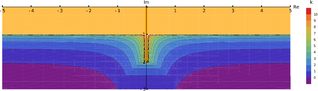
Figure 2. ​Level curves of the resolvent norm bound in Theorem 2.3 for the case εmin=μmin=1\varepsilon_{\min}\!=\!\mu_{\min}\!=\!1, σmax=2\sigma_{\max}\!=\!2, also for regions inside the numerical range W⁡(V)={z∈ℂ:Im⁡z∈[−2,0]}W(V)=\!\{z\!\in\!\mathbb{C}:\operatorname{Im}z\!\in\![-2,0]\} of the Maxwell pencil.

The next group of new results concerns approximations of the Maxwell pencil. Since Ω\Omega is a Lipschitz domain, we may assume that there exists a strictly increasing sequence of bounded Lipschitz domains (Ωn)n∈ℕ(\Omega_{n})_{n\in\mathbb{N}} such that ⋃n∈ℕΩn=Ω\bigcup_{n\in\mathbb{N}}\Omega_{n}=\Omega.

It is clear that if Ω=ℝ3\Omega=\mathbb{R}^{3}, or Ω\Omega has smooth boundary, we may choose Ωn\Omega_{n} to be smooth domains for every n∈ℕn\in\mathbb{N}. We note that sequences of domains (Ωn)n∈ℕ(\Omega_{n})_{n\in\mathbb{N}} as described above can always be constructed by setting Ωn=Ω∩B⁡(0,n)\Omega_{n}=\Omega\cap B(0,n), n∈ℕn\in\mathbb{N}.

Define Vn​(⋅)V_{n}(\cdot) to be the Maxwell pencil in L2​(Ωn)3⊕L2​(Ωn)3L^{2}(\Omega_{n})^{3}\oplus L^{2}(\Omega_{n})^{3} with domain

dom⁡(Vn​(ω))=H0​(curl,Ωn)⊕H⁡(curl,Ωn),ω∈ℂ,n∈ℕ,\operatorname{dom}(V_{n}(\omega))=H_{0}(\curl,\Omega_{n})\oplus H(\curl,\Omega_{n}),\ \omega\in\mathbb{C},\quad n\in\mathbb{N},

and the set of spectral pollution for the domain truncation method (Vn)n∈ℕ(V_{n})_{n\in\mathbb{N}} as

σpoll((Vn)n∈ℕ):={ω∈ℂ:ω∈ϱ(V),∃ωn∈σ(Vn):ωn→ω}.\sigma_{\rm poll}((V_{n})_{n\in\mathbb{N}}):=\{\omega\in\mathbb{C}:\omega\in\varrho(V),\exists\,\omega_{n}\in\sigma(V_{n}):\omega_{n}\to\omega\}. (2.7)

For approximations of an abstract linear pencil A−λ​BA-\lambda B, λ∈ℂ\lambda\in\mathbb{C}, spectral pollution for the domain truncation method was localised inside its essential numerical range in [10, Thm. 3.5]. For the Maxwell pencil V⁡(⋅)V(\cdot), it is not difficult to show that the essential numerical range We​(V)W_{e}(V) is contained in the closed horizontal strip {z∈ℂ:−σmaxεmin≤Im⁡z≤0}\{z\!\in\!\mathbb{C}:-\frac{\sigma_{\max}}{\varepsilon_{\min}}\!\leq\!\operatorname{Im}z\!\leq\!0\}.

Our second main result improves this enclosure substantially if we assume that the coefficients ε\varepsilon, μ\mu, σ\sigma have limits at ∞\infty. It shows that, in fact, spectral pollution is confined to the real axis, with possible gaps on either side of 00.

Theorem 2.4.

Suppose that Ω\Omega is an unbounded domain and that ε−ε∞​id\varepsilon\!-\!\varepsilon_{\infty}\operatorname{id}, μ−μ∞​id\mu\!-\!\mu_{\infty}\operatorname{id} and σ\sigma vanish at infinity for some ε∞\varepsilon_{\infty}, μ∞>0\mu_{\infty}>0,

i.e.

limR→∞{sup‖x‖>Rmax⁡(‖ε⁡(x)−ε∞​id‖,‖μ⁡(x)−μ∞​id‖,‖σ⁡(x)‖)}=0.\lim_{R\to\infty}\left\{\sup_{\|x\|>R}\max\,\big(\|\varepsilon(x)-\varepsilon_{\infty}\operatorname{id}\|,\|\mu(x)-\mu_{\infty}\operatorname{id}\|,\|\sigma(x)\|\big)\right\}=0. (2.8)

Let L∞L_{\infty} be the operator pencil in the subspace H⁡(div⁡0,Ω)H(\Div 0,\Omega) of L2​(Ω)3L^{2}(\Omega)^{3} defined by

L∞​(ω):=curl⁡μ∞−1​curl0−ω2​ε∞,\displaystyle L_{\infty}(\omega):=\curl\mu_{\infty}^{-1}\curl_{0}-\omega^{2}\varepsilon_{\infty},
dom⁡(L∞​(ω)):={E∈H0​(curl,Ω)∩H⁡(div⁡0,Ω):curl⁡E∈H⁡(curl,Ω)},\displaystyle\operatorname{dom}(L_{\infty}(\omega)):=\{E\in H_{0}(\curl,\Omega){\cap H(\Div 0,\Omega)}:\curl E\in H(\curl,\Omega)\},

and let 𝒲⁡(⋅)\mathcal{W}(\cdot) be the operator pencil in L2​(Ω)3L^{2}(\Omega)^{3} defined by 𝒲⁡(ω):=−ω⁡(ω​ε+i​σ)\mathcal{W}(\omega)\!:=\!-\omega(\omega\varepsilon+\mathrm{i}\sigma), ω∈ℂ\omega\!\in\!\mathbb{C}. Then, with

λe,minΩ:=min⁡σe​(curl⁡curl0|H⁡(div⁡0,Ω))≥0\lambda_{e,\min}^{\Omega}\!:=\!\min\sigma_{e}(\curl\curl_{0}|_{H(\Div 0,\Omega)})\geq 0,

σpoll((Vn)n∈ℕ)⊂We(L∞)=(−∞,−(λe,minΩε∞​μ∞)/2]∪[(λe,minΩε∞​μ∞)/2,∞)⊆ℝ;\sigma_{\rm poll}\big((V_{n})_{n\in\mathbb{N}}\big)\subset W_{e}(L_{\infty})\,=\Big(\!\!-\!\infty,\!-\Big(\frac{\lambda_{e,\min}^{\Omega}}{\varepsilon_{\infty}\mu_{\infty}}\Big)^{\!\!1\!/2}\,\Big]\cup\Big[\Big(\frac{\lambda_{e,\min}^{\Omega}}{\varepsilon_{\infty}\mu_{\infty}}\Big)^{\!\!1\!/2},\infty\Big)\\ \subseteq\mathbb{R};

and for every isolated ω∈σp​(V)\omega\in\sigma_{p}(V) outside We​(L∞)∪σe​(P∇​𝒲​(⋅)|∇H˙01​(Ω))W_{e}(L_{\infty})\cup\sigma_{e}(P_{\nabla}\mathcal{W}(\cdot)|_{\nabla\!\dot{H}^{1}_{0}(\Omega)}), and hence outside the set We​(L∞)∪i⁡[−σmaxεmin,0]W_{e}(L_{\infty})\!\cup\!\mathrm{i}\big[\!-\!\frac{\sigma_{\max}}{\varepsilon_{\min}},0\big], there exists a sequence ωn∈σ⁡(Vn)\omega_{n}\in\sigma(V_{n}), n∈ℕn\in\mathbb{N}, such that ωn→ω\omega_{n}\to\omega as n→∞n\to\infty.

The proof of Theorem 2.4 which relies on a combination of analytic and operator theoretic tools is given at the end of Section 7.

Remark 2.5.

The enclosure for spectral pollution in Theorem 2.4 is a subset of the spectral enclosure in Theorem 2.1 on the real axis, see (2.5), since λe,minΩ≥λminΩ≥0\lambda_{e,\min}^{\Omega}\geq\lambda_{\min}^{\Omega}\geq 0 and ε∞≤εmax\varepsilon_{\infty}\!\leq\!\varepsilon_{\max}, μ∞≤μmax\mu_{\infty}\!\leq\!\mu_{\max}.
Note that, depending on Ω\Omega, it may happen that λminΩ>0\lambda_{\min}^{\Omega}\!>\!0 or λe,minΩ>λminΩ≥0\lambda_{e,\min}^{\Omega}\!>\!\lambda_{\min}^{\Omega}\!\geq\!0; in the former case, both enclosures for the spectrum and spectral pollution have a gap on either side of 00, in the latter case, the enclosure for spectral pollution has a gap on either side of 00 and thus eigenvalues in these gaps are safe from spectral pollution.

As far as we know, Theorem 2.4 is new even in the self-adjoint case, see also Theorem 7.7. In the general case, it yields spectral exactness for every non-real, isolated eigenvalue of the Maxwell system and, if λe,minΩ>0\lambda_{e,\min}^{\Omega}\!>\!0, also for the real eigenvalues in the gaps of the essential spectrum to either side of 00.

The following examples illustrate our results on spectral enclosure, the essential spectrum and spectral pollution. The first example also provides an idea of the complex spectral structure that may arise even for rather simple Maxwell systems (1).

Example 2.6.

We consider the semi-infinite cylinder Ω=(0,∞)×(0,L2)×(0,L3)\Omega=(0,\infty)\times(0,L_{2})\times(0,L_{3}) and suppose that ε=μ=id\varepsilon=\mu=\operatorname{id} everywhere, and σ=id\sigma=\operatorname{id} if x1∈(0,1)x_{1}\in(0,1), else σ=0\sigma=0, i.e. σ=χK​id\sigma\!=\!\chi_{K}\operatorname{id} with K:=(0,1)×(0,L2)×(0,L3)K:=(0,1)\times(0,L_{2})\times(0,L_{3}), so that the Maxwell pencil V⁡(⋅)V(\cdot) is non-self-adjoint with piecewise constant coefficients.

In the Appendix we show how Fourier expansion for EE together with [2, Thm. 6], or Theorem 5.5 below, can be used to deduce that the essential spectrum of VV in the infinite half-cylinder Ω\Omega coincides with the essential spectrum for the infinite cylinder ℝ×(0,L2)×(0,L3)\mathbb{R}\times(0,L_{2})\times(0,L_{3}) and hence satisfies

σe(V)=(−∞,−π/L]∪[π/L,+∞)∪(−i{0,1/2,1}),L=max{L2,L3}.\sigma_{e}(V)=(-\infty,-\pi/L]\cup[\pi/L,+\infty)\cup(-{\rm i}\{0,1/2,1\}),\quad L=\max\{L_{2},L_{3}\}. (2.9)

Now we truncate the domain to Ωn:=(0,Xn)×(0,L2)×(0,L3)\Omega_{n}:=(0,X_{n})\times(0,L_{2})\times(0,L_{3}), with Xn≫1X_{n}\gg 1 and let Vn​(⋅)V_{n}(\cdot) be the corresponding Maxwell pencil in (1). It turns out that ω∈ℂ\omega\in\mathbb{C} is an eigenvalue of Vn​(⋅)V_{n}(\cdot) if and only if, for some 𝐧=(n2,n3)∈ℕ2{\bf n}=(n_{2},n_{3})\in{\mathbb{N}}^{2} with |𝐧|>0|{\bf n}|>0,

α𝐧​(ω)​coth⁡(α𝐧​(ω))+β𝐧​(ω)​coth⁡(β𝐧​(ω)​(Xn−1))=0,n∈ℕ;\alpha_{\bf n}(\omega)\coth(\alpha_{\bf n}(\omega))+\beta_{\bf n}(\omega)\coth(\beta_{\bf n}(\omega)(X_{n}-1))=0,\quad n\!\in\!\mathbb{N}; (2.10)

the construction of the eigenfunctions is given in the appendix. Here

α𝐧​(ω):=π2​n22/L22+π2​n32/L32−ω⁡(ω+i),\displaystyle\alpha_{\bf n}(\omega):=\sqrt{\pi^{2}n_{2}^{2}/L_{2}^{2}+\pi^{2}n_{3}^{2}/L_{3}^{2}-\omega(\omega+\mathrm{i})}, (2.11)
β𝐧​(ω):=π2​n22/L22+π2​n32/L32−ω2,\displaystyle\beta_{\bf n}(\omega):=\sqrt{\pi^{2}n_{2}^{2}/L_{2}^{2}+\pi^{2}n_{3}^{2}/L_{3}^{2}-\omega^{2}},

where the branch of the square root is taken with non-negative real part. Note that there are no square root singularities since z↦z​coth⁡(z)z\mapsto z\coth(z) is a meromorphic function.

A little change in the Fourier ansatz allows us to also compute the eigenvalues of the problem in the whole domain Ω=(0,∞)×(0,L2)×(0,L3)\Omega=(0,\infty)\times(0,L_{2})\times(0,L_{3}); the eigenvalue equation for ω∈σp​(V)\omega\in\sigma_{p}(V) becomes

α𝐧​(ω)​coth⁡(α𝐧​(ω))+β𝐧​(ω)=0,𝐧=(n2,n3)∈ℕ2,|𝐧|>0,\alpha_{\bf n}(\omega)\coth(\alpha_{\bf n}(\omega))+\beta_{\bf n}(\omega)=0,\quad{\bf n}=(n_{2},n_{3})\in\mathbb{N}^{2},\,|{\bf n}|>0, (2.12)

which is also obtained from (2.10) in the limit

Xn→∞X_{n}\to\infty.

Refer to caption
Figure 3. Spectrum of VV in Ω=(0,∞)×(0,1)×(0,2)\Omega\!=\!(0,\infty)\!\times\!(0,1)\!\times\!(0,2). The essential spectrum is in red, the eigenvalues in blue. The yellow region is the enclosure in Theorem 2.1 for the eigenvalues away from i​ℝ{\rm i}\mathbb{R} and ℝ\mathbb{R}.
Refer to caption
Refer to caption
Figure 4. Eigenvalues of VV in Ω50=(0,50)×(0,1)×(0,2)\Omega_{50}=(0,50)\times(0,1)\times(0,2), ε=μ=id\varepsilon=\mu=\operatorname{id}, σ⁡(x)=χ(0,1)​(x1)\sigma(x)=\chi_{(0,1)}(x_{1}). The yellow area is the spectral enclosure given by Theorem 2.1. The picture below is a zoom in the area [0,32​π]+i⁡[−0.1,0][0,\frac{3}{2}\pi]+\mathrm{i}[-0.1,0].

The solutions to equations (2.12) and (2.10) can be plotted using a standard computational routine, see Figures 3 and 4. There are many isolated eigenvalues in the region ℝ×−i[0,1/2]\mathbb{R}\times-\mathrm{i}[0,1/2] that seem to lie along determined curves, see Figure 3. Let us give a brief idea of what these curves are. Provided that α𝐧​(ω)≠0\alpha_{\bf n}(\omega)\neq 0 and ω≠0\omega\neq 0, we rewrite the eigenvalue equation (2.12) in the form

coth⁡(α𝐧​(ω))=−β𝐧​(ω)α𝐧​(ω)=−1+i​ωπ2​n22/L22+π2​n32/L32−ω2−i​ω.\coth(\alpha_{\bf n}(\omega))=-\frac{\beta_{\bf n}(\omega)}{\alpha_{\bf n}(\omega)}=-\sqrt{1+\frac{\mathrm{i}\omega}{\pi^{2}n_{2}^{2}/L_{2}^{2}+\pi^{2}n_{3}^{2}/L_{3}^{2}-\omega^{2}-\mathrm{i}\omega}}.

We follow an eigenvalue branch (ωk)k(\omega_{k})_{k} which we write as ωk=μk+i(−1/2+δk)\omega_{k}=\mu_{k}+\mathrm{i}(-1/2+\delta_{k}) with μk∈ℝ\mu_{k}\in\mathbb{R} and δk∈[0,1/2]\delta_{k}\in[0,1/2]. We show that, if |μk|→∞|\mu_{k}|\to\infty, then there exists a subsequence for which δk→0\delta_{k}\to 0 as k→∞k\to\infty. Without loss of generality, let μk→∞\mu_{k}\to\infty. We assume that lim infk→∞δk>0\liminf_{k\to\infty}\delta_{k}\!>\!0 and show that this leads to a contradiction. Clearly,

ωk​(ωk+i)=(ωk+i/2)2+1/4=μk2+1/4−δk2+i​2​μk​δk;\omega_{k}(\omega_{k}+\mathrm{i})=(\omega_{k}+\mathrm{i}/2)^{2}+1/4=\mu_{k}^{2}+1/4-\delta_{k}^{2}+\mathrm{i}2\mu_{k}\delta_{k};

note that the corresponding 𝐧{\bf n} for which ωk\omega_{k} satisfies (2.12) may depend on kk. If we set ck:=π2​n22/L22+π2​n32/L32>0c_{k}:=\pi^{2}n_{2}^{2}/L_{2}^{2}+\pi^{2}n_{3}^{2}/L_{3}^{2}>0, then

α𝐧​(ωk)\displaystyle\alpha_{\bf n}(\omega_{k}) =ck−μk2−1/4+δk2−i2​μk​δk,\displaystyle=\sqrt{c_{k}-\mu_{k}^{2}-1/4+\delta_{k}^{2}-\mathrm{i}2\mu_{k}\delta_{k}},
coth⁡(α𝐧​(ωk))\displaystyle\coth(\alpha_{\bf n}(\omega_{k})) =−1+1/2−δk+i​μkck−μk2−1/4+δk2−i​2​μk​δk.\displaystyle=-\sqrt{1+\frac{1/2-\delta_{k}+\mathrm{i}\mu_{k}}{c_{k}-\mu_{k}^{2}-1/4+\delta_{k}^{2}-\mathrm{i}2\mu_{k}\delta_{k}}}.

If |ck−μk2|≫μk|c_{k}-\mu_{k}^{2}|\gg\mu_{k}, then coth⁡(α𝐧​(ωk))→−1\coth(\alpha_{\bf n}(\omega_{k}))\to-1 as k→∞k\to\infty and

Re⁡α𝐧​(ωk)∼{ck−μk2if ​ck−μk2→∞,μk​δk|ck−μk2|if ​ck−μk2→−∞;\operatorname{Re}\alpha_{\bf n}(\omega_{k})\sim\begin{cases}\sqrt{c_{k}-\mu_{k}^{2}}\ &\text{if }c_{k}-\mu_{k}^{2}\to\infty,\\ \ \frac{\mu_{k}\delta_{k}}{\sqrt{|c_{k}-\mu_{k}^{2}|}}\ &\text{if }c_{k}-\mu_{k}^{2}\to-\infty;\end{cases}

note that coth⁡(α𝐧​(ωk))→−1\coth(\alpha_{\bf n}(\omega_{k}))\to-1 requires Re⁡α𝐧​(ωk)→−∞\operatorname{Re}\alpha_{\bf n}(\omega_{k})\to-\infty, but in both cases we have Re⁡α𝐧​(ωk)>0\operatorname{Re}\alpha_{\bf n}(\omega_{k})>0 asymptotically. It remains to consider the case |ck−μk2|=O⁡(μk)|c_{k}-\mu_{k}^{2}|={\rm O}(\mu_{k}). By the assumption lim infk→∞δk≠0\liminf_{k\to\infty}\delta_{k}\neq 0, there is a subsequence on which ck−μk2−1/4+δk2−i​2​μk​δk∼C​μkc_{k}-\mu_{k}^{2}-1/4+\delta_{k}^{2}-\mathrm{i}2\mu_{k}\delta_{k}\sim C\mu_{k} with Im⁡C≠0\operatorname{Im}C\neq 0. Then coth⁡(α𝐧​(ωk))→−1+i/C\coth(\alpha_{\bf n}(\omega_{k}))\to-\sqrt{1+\mathrm{i}/C}. But Re⁡α𝐧​(ωk)∼Re⁡(C)​μk→±∞\operatorname{Re}\alpha_{\bf n}(\omega_{k})\sim\operatorname{Re}(\sqrt{C})\sqrt{\mu_{k}}\to\pm\infty implies that coth⁡(α𝐧​(ωk))→±1\coth(\alpha_{\bf n}(\omega_{k}))\to\pm 1. The obtained contradiction proves lim infk→∞δk=0\liminf_{k\to\infty}\delta_{k}=0.

For this example, we therefore see that the presence of the compactly supported conductivity generates infinitely many eigenvalues, both in unbounded and bounded domains. These eigenvalues are approximated without spectral pollution due to our result Theorem 2.4, since in this example We​(L∞)W_{e}(L_{\infty}) and σe​(P∇​𝒲​(⋅)|∇H˙01​(Ω))\sigma_{e}(P_{\nabla}\mathcal{W}(\cdot)|_{\nabla\!\dot{H}^{1}_{0}(\Omega)}) are subsets of the essential spectrum of VV.

Moreover, one can verify that λminΩ=π2/L2\lambda_{\min}^{\Omega}\!=\!\pi^{2}/L^{2}. This and the fact that the eigenvalues approach the line Imω=−1/2\operatorname{Im}\omega=-1/2 as |x|→∞|x|\to\infty show that our spectral enclosure in Theorem 2.1 is sharp.

Example 2.7.

In the case of zero conductivity the Maxwell pencil is self-adjoint. Taking the same domain Ω\Omega as in Example 2.6, but now with coefficients μ=id\mu\!=\!\operatorname{id}, σ=0\sigma\!=\!0 and ε=(1+δ)​id\varepsilon\!=\!(1+\delta)\operatorname{id} with constant δ>0\delta>0 if x1∈(0,1)x_{1}\in(0,1), else ε=id\varepsilon\!=\operatorname{id}, i.e. ε=(1+δ​χK)​id\varepsilon=(1+\delta\,\chi_{K})\operatorname{id} with KK as in Example 2.6, we lose the imaginary part of the essential spectrum from Example 2.6, leaving just

σe(V)=(−∞,−π/L]∪{0}∪[π/L,+∞),L=max{L2,L3}.\sigma_{e}(V)=(-\infty,-\pi/L]\cup\{0\}\cup[\pi/L,+\infty),\quad L=\max\{L_{2},L_{3}\}. (2.13)

By calculations similar to those which led to equation (2.12), the eigenvalues are the real zeros of the set of analytic functions

ω↦α~𝐧​(ω)​coth⁡(α~𝐧​(ω))+β𝐧​(ω),𝐧=(n2,n3)∈ℕ2,|𝐧|>0,\omega\mapsto\tilde{\alpha}_{\bf n}(\omega)\coth(\tilde{\alpha}_{\bf n}(\omega))+\beta_{\bf n}(\omega),\quad{\bf n}=(n_{2},n_{3})\in\mathbb{N}^{2},\,|{\bf n}|>0, (2.14)

in which now α~𝐧​(ω)=π2​n22/L22+π2​n32/L32−(1+δ)​ω2\tilde{\alpha}_{\bf n}(\omega)=\sqrt{\pi^{2}n_{2}^{2}/L_{2}^{2}+\pi^{2}n_{3}^{2}/L_{3}^{2}-(1+\delta)\omega^{2}}. Taking L2=1L_{2}=1, L3=2L_{3}=2 and δ=10\delta=10, we have σe(V)=(−∞,−π/2]∪{0}∪[π/2,+∞)\sigma_{e}(V)=(-\infty,-\pi/2]\cup\{0\}\cup[\pi/2,+\infty). Elementary numerics show that the gap (−π/2,π/2)(-\pi/2,\pi/2) contains four eigenvalues, given approximately by ±1.4622\pm 1.4622 (both simple) and ±1.5643\pm 1.5643 (both multiplicity 2). These eigenvalues can be approximated without pollution using a domain truncation method: this follows immediately from Theorem 2.4, by verifying that λe,minΩ=π2/4\lambda_{e,\min}^{\Omega}=\pi^{2}/4 and since σe​(P∇​𝒲​(⋅)|∇H˙01​(Ω))={0}⊂σe​(V)\sigma_{e}(P_{\nabla}\mathcal{W}(\cdot)|_{\nabla\!\dot{H}^{1}_{0}(\Omega)})=\{0\}\subset\sigma_{e}(V). It may also be seen from the fact that, just as in Example 2.6, the functions (2.14), whose zeros are the eigenvalues, are the locally uniform limits as n→∞n\to\infty of the functions

ω↦α~𝐧​(ω)​coth⁡(α~𝐧​(ω))+β𝐧​(ω)​coth⁡(β𝐧​(ω)​(Xn−1)),\omega\mapsto\tilde{\alpha}_{\bf n}(\omega)\coth(\tilde{\alpha}_{\bf n}(\omega))+\beta_{\bf n}(\omega)\coth(\beta_{\bf n}(\omega)(X_{n}-1)),

whose zeros are the eigenvalues for the truncated domains. Thus we have a total absence of spectral pollution in this self-adjoint example despite the fact that, by [11, Thm. 3.8], it has We​(V)=ℝW_{e}(V)=\mathbb{R}.

3. Proofs of the spectral enclosure result and resolvent estimate

In this section we prove the spectral enclosure in Theorem 2.1 and the resolvent estimate in Theorem 2.3. We also show some auxiliary results that are used for the spectral pollution result.

Since ε\varepsilon and μ\mu are bounded and uniformly positive, the linear Maxwell pencil V⁡(⋅)V(\cdot) in (2.4) admits the factorisation

V⁡(ω)=(ε1/200μ1/2)⁡(𝒜−ω​I)​(ε1/200μ1/2),V(\omega)=\begin{pmatrix}\varepsilon^{1/2}&0\\ 0&\mu^{1/2}\end{pmatrix}(\mathcal{A}-\omega I)\begin{pmatrix}\varepsilon^{1/2}&0\\ 0&\mu^{1/2}\end{pmatrix}, (3.1)

in which

\displaystyle 𝒜:=(−i​ε−12​σ​ε−12−iε−12curlμ−1/2iμ−1/2curl0ε−120),\displaystyle\mathcal{A}:=\begin{pmatrix}-\mathrm{i}\varepsilon^{-\frac{1}{2}}\sigma\varepsilon^{-\frac{1}{2}}&-\mathrm{i}\varepsilon^{-\frac{1}{2}}\curl\mu^{-1/2}\\ \mathrm{i}\mu^{-1/2}{\curl_{0}}\varepsilon^{-\frac{1}{2}}&0\end{pmatrix}, (3.2)
dom⁡(𝒜):=ε1/2​H0​(curl,Ω)⊕μ1/2​H​(curl,Ω).\displaystyle\operatorname{dom}(\mathcal{A}):=\varepsilon^{1/2}H_{0}(\curl,\Omega)\oplus\mu^{1/2}H(\curl,\Omega).
Proof of Theorem 2.1..

Since the matrix multiplication operators ε\varepsilon and μ\mu are bounded and uniformly positive, V⁡(ω)V(\omega) is bijective if and only if so is 𝒜−ω{\mathcal{A}}-\omega, and hence σ⁡(V)=σ⁡(𝒜)\sigma(V)=\sigma(\mathcal{A}). Observe that

𝒜−ω=(−iε−1/2σε−1/2−ωiε−1/2curlμ−1/2−iμ−1/2curl0ε−1/2−ω)=:(−i​QBB∗0)−ω;\displaystyle\mathcal{A}-\omega=\begin{pmatrix}-\mathrm{i}\varepsilon^{-1/2}\sigma\varepsilon^{-1/2}-\omega\!&\!\mathrm{i}\varepsilon^{-1/2}\curl\mu^{-1/2}\\ -\mathrm{i}\mu^{-1/2}\curl_{0}\varepsilon^{-1/2}\!&\!-\omega\end{pmatrix}=:\begin{pmatrix}-\mathrm{i}Q&B\\ B^{*}&0\end{pmatrix}-\omega; (3.3)

note that (μ−1/2curl0ε−1/2)∗=ε−1/2curlμ−1/2(\mu^{-1/2}\curl_{0}\varepsilon^{-1/2})^{*}=\varepsilon^{-1/2}\curl\mu^{-1/2} since μ−1/2\mu^{-1/2} is bounded and ε−1/2\varepsilon^{-1/2} is bounded with range equal to the whole space, see [24]. Since 𝒜\mathcal{A} is a bounded perturbation of the self-adjoint off-diagonal part of 𝒜\mathcal{A}, it is obvious that both the upper and lower half-plane contain at least one point of the resolvent set of 𝒜\mathcal{A}. Hence it suffices to prove the claimed enclosures for the approximate point spectrum σa​p​p​(𝒜)\sigma_{app}(\mathcal{A}).

So let ω∈σa​p​p​(𝒜)\omega\!\in\!\sigma_{app}(\mathcal{A}). Then there exists a sequence ((fn,gn)t)n∈ℕ⊂dom⁡(B∗)⊕dom⁡(B)((f_{n},g_{n})^{t})_{n\in\mathbb{N}}\!\subset\!\operatorname{dom}(B^{*})\oplus\operatorname{dom}(B), ∥fn∥2+∥gn∥2=1\lVert f_{n}\rVert^{2}+\lVert g_{n}\rVert^{2}=1, with

(−i​Q−ω)​fn+B​gn\displaystyle(-\mathrm{i}Q-\omega)f_{n}+Bg_{n} =:hn→0,n→∞,\displaystyle=:h_{n}\to 0,\quad n\to\infty, (3.4)
B∗​fn−ω​gn\displaystyle B^{*}f_{n}-\omega g_{n} =:kn→0,n→∞.\displaystyle=:k_{n}\to 0,\quad n\to\infty. (3.5)

If ω=0\omega\!=\!0, there is nothing to show. Hence we can suppose that ω≠0\omega\!\neq\!0. In this case fn≠0f_{n}\!\neq\!0 for sufficiently large n∈ℕn\!\in\!\mathbb{N} since otherwise (3.5) would imply the contradiction gn→0g_{n}\!\to\!0, n→∞n\!\to\!\infty; hence, without loss of generality we can assume that fn≠0f_{n}\!\neq\!0, n∈ℕn\!\in\!\mathbb{N}.

If we decompose gn=gn1+gn2g_{n}=g_{n}^{1}+g_{n}^{2} with gn1∈(ker⁡B)⟂g_{n}^{1}\in(\ker B)^{\perp}, gn2∈ker⁡B=(ran⁡B∗)⟂g_{n}^{2}\in\ker B=(\operatorname{ran}B^{*})^{\perp}, then ∥gn1∥2+∥gn2∥2=∥gn∥2≤1\lVert g_{n}^{1}\rVert^{2}+\lVert g_{n}^{2}\rVert^{2}=\lVert g_{n}\rVert^{2}\leq 1, n∈ℕn\in\mathbb{N}. Now we take the scalar products with gn1g_{n}^{1} and gn2g_{n}^{2}, respectively, in (3.5), to conclude

that

⟨B∗​fn,gn1⟩−ω⁡⟨gn1,gn1⟩\displaystyle\langle B^{*}f_{n},g_{n}^{1}\rangle-\omega\langle g_{n}^{1},g_{n}^{1}\rangle =⟨kn,gn1⟩→0,n→∞,\displaystyle=\langle k_{n},g_{n}^{1}\rangle\to 0,\quad n\to\infty, (3.6)
−ω⁡⟨gn2,gn2⟩\displaystyle-\omega\langle g_{n}^{2},g_{n}^{2}\rangle =⟨kn,gn2⟩→0,n→∞.\displaystyle=\langle k_{n},g_{n}^{2}\rangle\to 0,\quad n\to\infty. (3.7)

Taking the scalar product with fnf_{n} in (3.4), we arrive at

⟨(−i​Q−ω)​fn,fn⟩+⟨B​gn1,fn⟩=⟨hn,fn⟩→0,n→∞.\langle(-\mathrm{i}Q-\omega)f_{n},f_{n}\rangle+\langle Bg_{n}^{1},f_{n}\rangle=\langle h_{n},f_{n}\rangle\to 0,\quad n\to\infty. (3.8)

If we subtract the real part of (3.8) from the real part of (3.6), it follows that

−Re⁡ω​∥gn1∥2−Re⁡⟨(−i​Q−ω)​fn,fn⟩=Re⁡(⟨kn,gn1⟩−⟨hn,fn⟩)→0,n→∞.-\operatorname{Re}\omega\lVert g_{n}^{1}\rVert^{2}-\operatorname{Re}\langle(-\mathrm{i}Q-\omega)f_{n},f_{n}\rangle=\operatorname{Re}\big(\langle k_{n},g_{n}^{1}\rangle-\langle h_{n},f_{n}\rangle\big)\to 0,\quad n\to\infty.

Since Q=ε−1/2σε−1/2Q=\varepsilon^{-1/2}\sigma\varepsilon^{-1/2} is a self-adjoint matrix multiplication operator, this implies

Re⁡ω⁡(∥fn∥2−∥gn1∥2)→0,n→∞.\displaystyle\operatorname{Re}\omega\big(\lVert f_{n}\rVert^{2}-\lVert g_{n}^{1}\rVert^{2}\big)\to 0,\quad n\to\infty. (3.9)

If we add the imaginary parts of (3.6) and (3.8), we obtain

−Im⁡ω​∥gn1∥2+Im⁡⟨(−i​Q−ω)​fn,fn⟩=Im⁡(⟨kn,gn1⟩+⟨hn,fn⟩)→0,n→∞,-\operatorname{Im}\omega\lVert g_{n}^{1}\rVert^{2}+\operatorname{Im}\langle(-\mathrm{i}Q-\omega)f_{n},f_{n}\rangle=\operatorname{Im}\big(\langle k_{n},g_{n}^{1}\rangle+\langle h_{n},f_{n}\rangle\big)\to 0,\quad n\to\infty,

and hence

(Im⁡ω)​(∥gn1∥2+∥fn∥2)+⟨Q​fn,fn⟩→0,n→∞.\displaystyle(\operatorname{Im}\omega)\big(\lVert g_{n}^{1}\rVert^{2}+\lVert f_{n}\rVert^{2}\big)+\langle Qf_{n},f_{n}\rangle\to 0,\quad n\to\infty. (3.10)

Since ∥fn∥2+∥gn1∥2+∥gn2∥2=∥fn∥2+∥gn∥2=1\lVert f_{n}\rVert^{2}+\lVert g_{n}^{1}\rVert^{2}+\lVert g_{n}^{2}\rVert^{2}=\lVert f_{n}\rVert^{2}+\lVert g_{n}\rVert^{2}=1 and ∥gn2∥2→0\lVert g_{n}^{2}\rVert^{2}\to 0, n→∞n\to\infty, by (3.7), we have ∥fn∥2+∥gn1∥2→1\lVert f_{n}\rVert^{2}+\lVert g_{n}^{1}\rVert^{2}\to 1, n→∞n\to\infty; hence we can assume without loss of generality that ∥fn∥2+∥gn1∥2≥c1>0\lVert f_{n}\rVert^{2}+\lVert g_{n}^{1}\rVert^{2}\geq c_{1}>0 with c1∈(0,1]c_{1}\in(0,1].

Since ω≠0\omega\neq 0, either (3.9) or (3.10) shows that fn→0f_{n}\to 0, n→∞n\to\infty, implies the contradiction ∥gn1∥→0\lVert g_{n}^{1}\rVert\to 0, n→∞n\to\infty. Hence, if ω≠0\omega\neq 0, we can assume without loss of generality that ∥fn∥≥c2>0\lVert f_{n}\rVert\geq c_{2}>0 with c2∈(0,1]c_{2}\in(0,1]. Then (3.10) can be equivalently written

as

∥fn∥2∥gn1∥2+∥fn∥2⏟∈[0,1]​⟨Q​fn,fn⟩∥fn∥2⏟∈W⁡(Q)→−Im⁡ω,n→∞.\displaystyle\underbrace{\frac{\lVert f_{n}\rVert^{2}}{\lVert g_{n}^{1}\rVert^{2}+\lVert f_{n}\rVert^{2}}}_{\in[0,1]}\underbrace{\frac{\langle Qf_{n},f_{n}\rangle}{\lVert f_{n}\rVert^{2}}}_{\in W(Q)}\to-\operatorname{Im}\omega,\quad n\to\infty. (3.11)

Since QQ is self-adjoint, its numerical range W(Q):={⟨Qf,f⟩:f∈L2(Ω)3,∥f∥=1}W(Q)\!:=\!\{\langle Qf,f\rangle:f\in L^{2}(\Omega)^{3},\|f\|=1\} satisfies W⁡(Q)=conv​σ​(Q)⊂[0,σmaxεmin]W(Q)\!=\!{\rm conv}\,\sigma(Q)\!\subset\!\big[0,\frac{\sigma_{\max}}{\varepsilon_{\min}}\big]

and thus (3.11) implies

Im⁡ω∈−conv⁡(OPENW⁡(Q)∪{0})¯=[−σmaxεmin,0]CLOSE,\operatorname{Im}\omega\in-{\rm conv}\,\big(\overline{W(Q)\cup\{0\}\big)}=\Big[-\frac{\sigma_{\max}}{\varepsilon_{\min}},0\Big],

which proves the claimed estimate on the imaginary axis.

Now suppose that ω∈ℂ∖i​ℝ\omega\in\mathbb{C}\setminus\mathrm{i}\mathbb{R}, i.e. Re⁡ω≠0\operatorname{Re}\omega\neq 0. Then (3.9) implies that

∥fn∥2−∥gn1∥2→0,n→∞.\lVert f_{n}\rVert^{2}-\lVert g_{n}^{1}\rVert^{2}\to 0,\quad n\to\infty. (3.12)

Noting that (∥fn∥2+∥gn1∥2)−2​∥fn∥2=∥gn1∥2−∥fn∥2→0\big(\lVert f_{n}\rVert^{2}+\lVert g_{n}^{1}\rVert^{2}\big)-2\lVert f_{n}\rVert^{2}=\lVert g_{n}^{1}\rVert^{2}-\lVert f_{n}\rVert^{2}\to 0, n→∞n\to\infty (due to (3.12)) and using this in (3.10), we obtain that

2​Im⁡ω​∥fn∥2+⟨Q​fn,fn⟩→0,n→∞,\displaystyle 2\operatorname{Im}\omega\lVert f_{n}\rVert^{2}+\langle Qf_{n},f_{n}\rangle\to 0,\quad n\to\infty, (3.13)

and

hence

−12​⟨Q​fn,fn⟩∥fn∥2⏟∈W⁡(Q)→Im⁡ω,n→∞.\displaystyle-\frac{1}{2}\underbrace{\frac{\langle Qf_{n},f_{n}\rangle}{\lVert f_{n}\rVert^{2}}}_{\in W(Q)}\to\operatorname{Im}\omega,\quad n\to\infty.

This proves that

ω∈ℂ∖i​ℝ⟹Im⁡ω∈−12​W⁡(Q)¯⊂[−12​σmaxεmin,−12​σminΩεmax].\displaystyle\omega\in\mathbb{C}\setminus\mathrm{i}\mathbb{R}\ \implies\ \operatorname{Im}\omega\in-\frac{1}{2}\overline{W(Q)}\subset\Big[-\frac{1}{2}\frac{\sigma_{\max}}{\varepsilon_{\min}},-\frac{1}{2}\frac{\sigma_{\min}^{\Omega}}{\varepsilon_{\max}}\Big]. (3.14)

In order to prove the second inequality for ω∈ℂ∖i​ℝ\omega\in\mathbb{C}\setminus\mathrm{i}\mathbb{R}, we use the reduced minimum modulus of a closed linear operator TT, defined by

γ⁡(T):=infx∈dom⁡T‖T​x‖dist⁡(x,ker⁡T),\gamma(T):=\inf_{x\in\operatorname{dom}T}\frac{\|Tx\|}{{\rm dist}(x,\ker T)},

see e.g. [25, Thm. IV.5.2, p. 231]. Note that γ⁡(T)>0\gamma(T)>0 if and only if ran⁡T\operatorname{ran}T is closed; in this case γ⁡(T)=∥T+∥−1\gamma(T)=\lVert T^{+}\rVert^{-1} where T+T^{+} is the Moore-Penrose inverse of TT, γ⁡(T)=γ⁡(T∗)\gamma(T)=\gamma(T^{*}), see [22, Cor. IV.1.9], and, if T≢0T\not\equiv 0,

γ​(T)2=min⁡(σ⁡(T∗​T)∖{0})=min⁡σ⁡(T∗​T|dom⁡(T∗​T)∩(ker⁡T)⟂),\displaystyle\gamma(T)^{2}=\min\big(\sigma(T^{*}T)\setminus\{0\}\big)=\min\sigma(T^{*}T|_{\operatorname{dom}(T^{*}T)\cap(\ker T)^{\perp}}), (3.15)

comp. [4] for the bounded case. In the unbounded case, T∗​TT^{*}T is self-adjoint and its dense domain dom⁡(T∗​T)\operatorname{dom}(T^{*}T) is a core for TT, see [25, Thm. V.3.24]. Hence

γ​(T)2\displaystyle\gamma(T)^{2} =infx∈dom⁡T∩(ker⁡T)⟂‖T​x‖2‖x‖2=infx∈dom⁡T∗​T∩(ker⁡T)⟂‖T​x‖2‖x‖\displaystyle=\inf_{x\in\operatorname{dom}T\cap(\ker T)^{\perp}}\frac{\|Tx\|^{2}}{\|x\|^{2}}=\inf_{x\in\operatorname{dom}T^{*}T\cap(\ker T)^{\perp}}\frac{\|Tx\|^{2}}{\|x\|}
=infx∈dom⁡T∗​T∩(ker⁡T)⟂(T∗​T​x,x)‖x‖2=min⁡σ⁡(T∗​T|dom⁡(T∗​T)∩(ker⁡T)⟂).\displaystyle=\inf_{x\in\operatorname{dom}T^{*}T\cap(\ker T)^{\perp}}\frac{(T^{*}Tx,x)}{\|x\|^{2}}=\min\sigma(T^{*}T|_{\operatorname{dom}(T^{*}T)\cap(\ker T)^{\perp}}).\vskip-28.45274pt

For B=iε−1/2curlμ−1/2B\!=\!\mathrm{i}\varepsilon^{-1/2}\curl\mu^{-1/2}, we have dom⁡B=μ1/2​H​(curl,Ω)\operatorname{dom}B\!=\!\mu^{1/2}H(\curl,\Omega), ker⁡B=μ1/2​ker⁡curl\ker B\!=\!\mu^{1/2}\ker\curl and thus

γ⁡(B)\displaystyle\gamma(B) =infx∈μ1/2​H​(curl,Ω)∥ε−1/2curlμ−1/2x∥dist⁡(x,μ1/2​ker⁡curl)=infu∈H⁡(curl,Ω)∥ε−1/2curlu∥dist⁡(μ1/2​u,μ1/2​ker⁡curl)\displaystyle=\!\!\inf_{x\in\mu^{1/2}H(\curl,\Omega)}\frac{\|\varepsilon^{-1/2}\curl\mu^{-1/2}x\|}{{\rm dist}(x,\mu^{1/2}\ker\curl)}=\!\!\inf_{u\in H(\curl,\Omega)}\frac{\|\varepsilon^{-1/2}\curl u\|}{{\rm dist}(\mu^{1/2}u,\mu^{1/2}\ker\curl)}
≥1εmax1/2​infu∈H⁡(curl,Ω)‖curl⁡u‖dist⁡(μ1/2​u,μ1/2​ker⁡curl)\displaystyle\geq\frac{1}{{\varepsilon_{\max}}^{\!\!\!\!\!1/2}}\inf_{u\in H(\curl,\Omega)}\frac{\|\curl u\|}{{\rm dist}(\mu^{1/2}u,\mu^{1/2}\ker\curl)}
≥1εmax1/2​μmax1/2​infu∈H⁡(curl,Ω)‖curl⁡u‖dist⁡(u,ker⁡curl)\displaystyle\geq\frac{1}{{\varepsilon_{\max}}^{\!\!\!\!\!1/2}{\mu_{\max}}^{\!\!\!\!\!1/2}}\inf_{u\in H(\curl,\Omega)}\frac{\|\curl u\|}{{\rm dist}(u,\ker\curl)}
=1εmax1/2​μmax1/2​γ​(curl)=1εmax1/2​μmax1/2​γ​(curl0).\displaystyle=\frac{1}{{\varepsilon_{\max}}^{\!\!\!\!\!1/2}{\mu_{\max}}^{\!\!\!\!\!1/2}}\,\gamma(\curl)=\frac{1}{{\varepsilon_{\max}}^{\!\!\!\!\!1/2}{\mu_{\max}}^{\!\!\!\!\!1/2}}\,\gamma(\curl_{0}).

Here, we have used γ⁡(T)=γ⁡(T∗)\gamma(T)=\gamma(T^{*}) to replace curl\curl by curl0\curl_{0} at the last step. Also, in the second estimate, we have used the equality

dist⁡(μ1/2​u,μ1/2​ker⁡curl)=infy∈ker⁡curl‖μ1/2​u−μ1/2​y‖≤μmax1/2​dist​(u,ker⁡curl).{\rm dist}\big(\mu^{1/2}u,\mu^{1/2}\ker\curl\big)=\inf\limits_{y\in\ker\curl}\big\|\mu^{1/2}u-\mu^{1/2}y\big\|\leq{\mu_{\max}}^{\!\!\!\!\!1/2}{\rm dist}(u,\ker\curl).

If λminΩ=0\lambda_{\min}^{\Omega}=0, then ran⁡curl0\operatorname{ran}\curl_{0} is not closed and hence γ⁡(curl0)=0\gamma(\curl_{0})=0. If λminΩ>0\lambda_{\min}^{\Omega}>0, then ran⁡curl0\operatorname{ran}\curl_{0} is closed and thus (ker⁡curl0)⟂=ran⁡curl⊂H⁡(div⁡0,Ω)(\ker\curl_{0})^{\perp}=\operatorname{ran}\curl\subset H(\Div 0,\Omega). Hence, by (3.15), in both cases, it follows

that

γ⁡(B)≥1εmax1/2​μmax1/2​λminΩ1/2.\displaystyle\gamma(B)\geq\frac{1}{{\varepsilon_{\max}}^{\!\!\!\!\!1/2}{\mu_{\max}}^{\!\!\!\!\!1/2}}{\lambda_{\min}^{\Omega}}^{\!\!\!\!\!1/2}. (3.16)

Now we can estimate

γ​(B)2​∥fn∥2\displaystyle\gamma(B)^{2}\lVert f_{n}\rVert^{2} =γ​(B)2​∥gn1∥2−γ​(B)2​(∥gn1∥2−∥fn∥2)≤‖B​gn1‖2−γ​(B)2​(∥gn1∥2−∥fn∥2)\displaystyle\!\!=\!\gamma(B)^{2}\lVert g_{n}^{1}\rVert^{2}\!-\!\gamma(B)^{2}\big(\lVert g_{n}^{1}\rVert^{2}\!-\!\lVert f_{n}\rVert^{2}\big)\!\leq\!\|Bg_{n}^{1}\|^{2}\!-\!\gamma(B)^{2}\big(\lVert g_{n}^{1}\rVert^{2}\!-\!\lVert f_{n}\rVert^{2}\big)

and further, since gn2∈ker⁡Bg_{n}^{2}\in\ker B and ‖fn‖≥c2\|f_{n}\|\geq c_{2} because ω≠0\omega\neq 0,

γ​(B)2\displaystyle\hskip-5.69054pt\gamma(B)^{2} ≤‖B​gn−(−i​Q−ω)​fn‖2‖fn‖2+‖(−i​Q−ω)​fn‖2‖fn‖2−γ​(B)2​∥gn1∥2−∥fn∥2‖fn‖2.\displaystyle\leq\frac{\|Bg_{n}\!-\!(-\mathrm{i}Q\!-\!\omega)f_{n}\|^{2}}{\|f_{n}\|^{2}}\!+\!\frac{\|(-\mathrm{i}Q\!-\!\omega)f_{n}\|^{2}}{\|f_{n}\|^{2}}\!-\!\gamma(B)^{2}\frac{\lVert g_{n}^{1}\rVert^{2}\!-\!\lVert f_{n}\rVert^{2}}{\|f_{n}\|^{2}}.\ \ (3.17)

For the middle term on the right-hand side we have

‖(−i​Q−ω)​fn‖2‖fn‖2=‖Q​fn‖2‖fn‖2+2​Im⁡ω​⟨Q​fn,fn⟩‖fn‖2+|ω|2.\displaystyle\frac{\|(-\mathrm{i}Q-\omega)f_{n}\|^{2}}{\|f_{n}\|^{2}}=\frac{\|Qf_{n}\|^{2}}{\|f_{n}\|^{2}}+2\operatorname{Im}\omega\frac{\langle Qf_{n},f_{n}\rangle}{\|f_{n}\|^{2}}+|\omega|^{2}. (3.18)

Using that QQ is self-adjoint, we can estimate

‖Q​fn‖2‖fn‖2=⟨Q​fn,Q​fn⟩‖fn‖2≤‖Q‖​⟨Q​fn,fn⟩‖fn‖2,n∈ℕ.\displaystyle\frac{\|Qf_{n}\|^{2}}{\|f_{n}\|^{2}}=\frac{\langle Qf_{n},Qf_{n}\rangle}{\|f_{n}\|^{2}}\leq\|Q\|\frac{\langle Qf_{n},f_{n}\rangle}{\|f_{n}\|^{2}},\quad n\in\mathbb{N}. (3.19)

Altogether, by (3.17), (3.18), (3.19) and since Im⁡ω≤0\operatorname{Im}\omega\leq 0 by (3.14), we arrive at

γ​(B)2≤(‖Q‖−2​|Im⁡ω|)​⟨Q​fn,fn⟩‖fn‖2+|ω|2\displaystyle\gamma(B)^{2}\!\leq\!\big(\|Q\|\!-\!2|\operatorname{Im}\omega|\big)\frac{\langle Qf_{n},f_{n}\rangle}{\|f_{n}\|^{2}}\!+\!|\omega|^{2} +‖B​gn−(−i​Q−ω)​fn‖2‖fn‖2\displaystyle\!+\!\frac{\|Bg_{n}\!-\!(-\mathrm{i}Q\!-\!\omega)f_{n}\|^{2}}{\|f_{n}\|^{2}}
−γ​(B)2​∥gn1∥2−∥fn∥2‖fn‖2.\displaystyle\!-\!\gamma(B)^{2}\frac{\lVert g_{n}^{1}\rVert^{2}\!-\!\lVert f_{n}\rVert^{2}}{\|f_{n}\|^{2}}.

If we use (3.13) and that by (3.4)and (3.12), the last two terms tend to 00, together with ∥Q∥=∥ε−1/2σε−1/2∥≤σmaxεmin\|Q\|=\|\varepsilon^{-1/2}\sigma\varepsilon^{-1/2}\|\leq\frac{\sigma_{\max}}{\varepsilon_{\min}}, we obtain

γ​(B)2≤(‖Q‖−2​|Im⁡ω|)​2​|Im⁡ω|+|ω|2=2​‖Q‖​|Im⁡ω|−3​|Im⁡ω|2+|Re⁡ω|2.\gamma(B)^{2}\leq\big(\|Q\|-2|\operatorname{Im}\omega|\big)2|\operatorname{Im}\omega|+|\omega|^{2}=2\|Q\||\operatorname{Im}\omega|-3|\operatorname{Im}\omega|^{2}+|\operatorname{Re}\omega|^{2}.

Now the remaining claimed inequality follows from (3.16). ∎

The following remark details the three different possible shapes of the spectral enclosure near the imaginary axis and the corresponding thresholds of λminΩ\lambda_{\min}^{\Omega}.

Remark 3.1.

Theorem 2.1 shows that σ⁡(V)∖i​ℝ\sigma(V)\setminus\mathrm{i}\mathbb{R} cannot approach σ⁡(V)∩i​ℝ⊂\sigma(V)\cap\mathrm{i}\mathbb{R}\subset i⁡[−σmaxεmin,0]\mathrm{i}\Big[\!\!-\!\!\tfrac{\sigma_{\max}}{\varepsilon_{\min}}\!,0\Big] in the lower half i⁡[−σmaxεmin,−12​σmaxεmin]\mathrm{i}\Big[\!\!-\!\!\tfrac{\sigma_{\max}}{\varepsilon_{\min}},\!-\!\tfrac{1}{2}\tfrac{\sigma_{\max}}{\varepsilon_{\min}}\Big] and that there are 3 thresholds

of λminΩ\lambda_{\min}^{\Omega} for where σ⁡(V)∖i​ℝ\sigma(V)\!\setminus\!\mathrm{i}\mathbb{R} may approach the upper half i⁡[−12​σmaxεmin,0]\mathrm{i}\Big[\!-\!\frac{1}{2}\frac{\sigma_{\max}}{\varepsilon_{\min}}\!,0\Big], see Figure 1:

i) if λminΩ>0\lambda_{\min}^{\Omega}\!>\!0, then σ⁡(V)∖i​ℝ\sigma(V)\!\setminus\!\mathrm{i}\mathbb{R} does not approach i⁡[−12​σmaxεmin,0]\mathrm{i}\Big[\!\!-\!\!\frac{1}{2}\frac{\sigma_{\max}}{\varepsilon_{\min}}\!,0\Big] near 00;

ii) if λminΩ>14​σmax2​εmax​μmaxεmin2\lambda_{\min}^{\Omega}\!>\!\frac{1}{4}\frac{\!\sigma_{\max}^{2}\varepsilon_{\max}\mu_{\max}\!}{\varepsilon_{\min}^{2}}\!, then σ⁡(V)∖i​ℝ\sigma(V)\!\setminus\mathrm{i}\mathbb{R} does not approach i⁡[−12​σmaxεmin,0]\mathrm{i}\Big[\!-\!\frac{1}{2}\frac{\sigma_{\max}}{\varepsilon_{\min}}\!,\!0\Big] near −i​12​σmaxεmin-\mathrm{i}\frac{1}{2}\frac{\sigma_{\max}}{\varepsilon_{\min}};

iii) ​if λminΩ>13​σmax2​εmax​μmaxεmin2\lambda_{\min}^{\Omega}\!>\!\frac{1}{3}\frac{\sigma_{\max}^{2}\varepsilon_{\max}\mu_{\max}}{\varepsilon_{\min}^{2}}, then σ⁡(V)∖i​ℝ\sigma(V)\!\setminus\!\mathrm{i}\mathbb{R} does not approach i⁡[−12​σmaxεmin,0]\mathrm{i}\Big[\!-\!\frac{1}{2}\frac{\sigma_{\max}}{\varepsilon_{\min}},0\Big] at all.

The following special case in Theorem 2.1 of constant matrix functions ε\varepsilon, σ\sigma, but still varying μ\mu, is useful e.g. for ‘limiting problems at ∞\infty’ if they exist.

Corollary 3.2.

If the matrix functions ε\varepsilon, σ\sigma are constant multiples of the identity, ε≡ε∞​id>0\varepsilon\!\equiv\!\varepsilon_{\infty}\operatorname{id}\!>\!0, σ≡σ∞​id≥0\sigma\!\equiv\!\sigma_{\infty}\operatorname{id}\!\geq\!0, then εmin=εmax=ε∞\varepsilon_{\min}\!=\!\varepsilon_{\max}\!=\!\varepsilon_{\infty}, σmin=σmax=σ∞\sigma_{\min}\!=\!\sigma_{\max}\!=\!\sigma_{\infty}

and thus

σ(V)⊂i[−σ∞ε∞,0]∪{ω∈ℂ∖iℝ:Imω=−12σ∞ε∞,(Reω)2+14σ∞2ε∞2≥λminΩε∞​μmax};\displaystyle\sigma(V)\subset\mathrm{i}\,\Big[\!-\!\frac{\sigma_{\infty}}{\varepsilon_{\infty}},0\Big]\cup\Big\{\omega\!\in\!\mathbb{C}\!\setminus\!\mathrm{i}\mathbb{R}:\operatorname{Im}\omega=-\frac{1}{2}\frac{\sigma_{\infty}}{\varepsilon_{\infty}},\ (\operatorname{Re}\omega)^{2}\!+\!\frac{1}{4}\frac{\sigma_{\infty}^{2}}{\varepsilon_{\infty}^{2}}\!\geq\!\frac{\lambda_{\min}^{\Omega}}{\varepsilon_{\infty}\mu_{\max}}\Big\};

in particular, σ⁡(V)∩i​ℝ⊂i⁡[−σ∞ε∞,0]\sigma(V)\cap\mathrm{i}\mathbb{R}\!\subset\!\mathrm{i}\big[\!-\!\frac{\sigma_{\infty}}{\varepsilon_{\infty}},0\big] is isolated from σ⁡(V)∖i​ℝ\sigma(V)\setminus\mathrm{i}\mathbb{R} if λminΩ>14​σ∞​μmaxε∞\lambda_{\min}^{\Omega}\!>\!\frac{1}{4}\frac{\sigma_{\infty}\mu_{\max}}{\varepsilon_{\infty}}.

Next we prove Theorem 2.3 providing a resolvent norm estimate of V⁡(⋅)V(\cdot).

Proof of Theorem 2.3..

Let ω∈ℂ∖i​ℝ\omega\!\in\!\mathbb{C}\!\setminus\!\mathrm{i}\mathbb{R}, Im⁡ω<−12​σmaxεmin\operatorname{Im}\omega\!<\!-\frac{1}{2}\frac{\sigma_{\max}}{\varepsilon_{\min}} or ω∈i​ℝ\omega\in\mathrm{i}\mathbb{R}, Im⁡ω<−σmaxεmin\operatorname{Im}\omega<-\frac{\sigma_{\max}}{\varepsilon_{\min}}. Then ω∈ϱ⁡(V)=ϱ⁡(𝒜)\omega\!\in\!\varrho(V)=\varrho(\mathcal{A}) by Theorem 2.1 and ‖V​(ω)−1‖≤1min⁡{εmin,μmin}​‖(𝒜−ω)−1‖\|V(\omega)^{-1}\|\!\leq\!\frac{1}{\min\{\varepsilon_{\min},\mu_{\min}\}}\|(\mathcal{A}\!-\!\omega)^{-1}\| due to the factorisation (3.1) where 𝒜\mathcal{A} is the operator matrix in (3.3). In order to estimate the resolvent of 𝒜\mathcal{A}, we continue to use the notation Q=ε−1/2σε−1/2Q\!=\!\varepsilon^{-1/2}\sigma\varepsilon^{-1/2}, B=ε−1/2curlμ−1/2B\!=\!\varepsilon^{-1/2}\curl\mu^{-1/2} introduced in (3.3).

Since 𝒜\mathcal{A} is a self-adjoint operator perturbed by the bounded operator diag⁡(−i​Q,0){\mathrm{diag}}(-\mathrm{i}Q,0) and W⁡(Q)⊂[0,qmax]W(Q)\!\subset\![0,q_{\max}] with qmax:=σmaxεminq_{\max}\!:=\!\frac{\sigma_{\max}}{\varepsilon_{\min}}, a numerical range argument for 𝒜\mathcal{A} yields the resolvent estimate ‖(𝒜−ω)−1‖≤1|Im⁡ω|−qmax\|(\mathcal{A}\!-\!\omega)^{-1}\|\leq\frac{1}{|\operatorname{Im}\omega|-q_{\max}} for all ω∈ℂ\omega\in\mathbb{C}, Im⁡ω<−qmax\operatorname{Im}\omega<-q_{\max}.

Now let ω=x+i​y\omega\!=\!x\!+\!\mathrm{i}y with x>0x\!>\!0, y<−qmax2y\!<\!-\frac{q_{\max}}{2}; the proof is analogous if x<0x\!<\!0. Let φ∈(0,π2)\varphi\in(0,\frac{\pi}{2}) be the argument of x+i​qmax2x+\mathrm{i}\frac{q_{\max}}{2}. Let ℬ=diag⁡(e−i​φ,ei​φ)\mathcal{B}={\mathrm{diag}}(\mathrm{e}^{-\mathrm{i}\varphi},\mathrm{e}^{\mathrm{i}\varphi}) in L2​(Ω)3⊕L2​(Ω)3L^{2}(\Omega)^{3}\oplus L^{2}(\Omega)^{3}, and let S:={z∈ℂ:arg⁡(z−γ)∈(−π+φ,−φ)}S\!:=\!\{z\in\mathbb{C}:{\rm arg}(z-\gamma)\in(-\pi+\varphi,-\varphi)\} be the open sector with vertex γ:=x−i​qmax/2\gamma\!:=\!x-\mathrm{i}q_{\max}/2 and semi-angle π2−φ\frac{\pi}{2}\!-\!\varphi. Note that ω∈S\omega\in S.

We claim that S∩W⁡(ℬ​𝒜,ℬ)=∅S\cap W(\mathcal{B}\mathcal{A},\mathcal{B})\!=\!\emptyset, where W⁡(ℬ​𝒜,ℬ):={z∈ℂ:∈W⁡(ℬ​𝒜−z​ℬ)¯}W(\mathcal{B}\mathcal{A},\mathcal{B})\!:=\!\{z\!\in\!\mathbb{C}:\,0\!\in\!\overline{W(\mathcal{B}\mathcal{A}\!-\!z\mathcal{B})}\}. Then [10, Thm. 4.1 ii)] implies S⊂ϱ⁡(𝒜)S\subset\varrho(\mathcal{A})

with

‖(𝒜−z)−1‖≤1cos⁡(φ)​dist⁡(z,∂S),z∈S.\|(\mathcal{A}-z)^{-1}\|\leq\frac{1}{\cos(\varphi)\,\operatorname{dist}(z,\partial S)},\quad z\in S.\vskip-4.2679pt
amax2\frac{a_{\max}}{2}−amax2-\frac{a_{\max}}{2}−amax-a_{\max}xxφ\varphiφ\varphiφ\varphiφ\varphiγ\gammazzz+i​amaxz+\mathrm{i}a_{\max}ω\omegaφ\varphiReIm
Figure 5. The geometry in the proof of Theorem 2.3: The blue line measures the distance of ω=x+i​y\omega\!=\!x\!+\!\mathrm{i}y to ∂S\partial S; since the lines meet at a right angle, the angle between the blue and the vertical dashed lines is also φ\varphi.

By means of Figure 5, one can check that for z=ωz\!=\!\omega we have dist⁡(z,∂S)=(|y|−qmax2)​cos⁡(φ)\operatorname{dist}(z,\partial S)\!=\!(|y|\!-\!\frac{q_{\max}}{2})\cos(\varphi) and cos2⁡(φ)=x2/(x2+(qmax2)2)\cos^{2}(\varphi)=x^{2}/(x^{2}+(\frac{q_{\max}}{2})^{2}), which

implies

‖(𝒜−ω)−1‖≤1|y|−qmax2​(1+(qmax2)2x2).\|(\mathcal{A}-\omega)^{-1}\|\leq\frac{1}{|y|-\frac{q_{\max}}{2}}\Big(1+\frac{(\frac{q_{\max}}{2})^{2}}{x^{2}}\Big).\vskip-2.84526pt

To prove that S∩W⁡(ℬ​𝒜,ℬ)=∅S\cap W(\mathcal{B}\mathcal{A},\mathcal{B})=\emptyset, assume that there exists z∈S∩W⁡(ℬ​𝒜,ℬ)z\in S\cap W(\mathcal{B}\mathcal{A},\mathcal{B}). This implies that there is a normalised sequence ((fn,gn)t)n∈ℕ⊂dom⁡(𝒜)((f_{n},g_{n})^{t})_{n\in\mathbb{N}}\subset\operatorname{dom}(\mathcal{A}) with ⟨ℬ⁡(𝒜−z)​(fn,gn)t,(fn,gn)t⟩→0\big\langle\mathcal{B}(\mathcal{A}-z)(f_{n},g_{n})^{t},(f_{n},g_{n})^{t}\big\rangle\to 0 as n→∞n\!\to\!\infty; in particular, the sequence also converges to 00 if we take imaginary parts. Let tn:=‖fn‖2∈[0,1]t_{n}:=\|f_{n}\|^{2}\in[0,1]. Then one can write ⟨Q​fn,fn⟩=an​tn\langle Qf_{n},f_{n}\rangle=a_{n}t_{n} for some an∈W⁡(Q)⊂[0,qmax]a_{n}\in W(Q)\subset[0,q_{\max}]. We obtain

Im⁡(tn​e−i​φ​(i​an+z)+(1−tn)​ei​φ​z)→0,n→∞.\operatorname{Im}\big(t_{n}\mathrm{e}^{-\mathrm{i}\varphi}(\mathrm{i}a_{n}+z)+(1-t_{n})\mathrm{e}^{\mathrm{i}\varphi}z\big)\to 0,\quad n\to\infty.

Note that we take convex linear combinations of points in e−i​φ​(z+i⁡[0,qmax])\mathrm{e}^{-\mathrm{i}\varphi}(z\!+\!\mathrm{i}[0,q_{\max}]) and {ei​φ​z}\{\mathrm{e}^{\mathrm{i}\varphi}z\}. Using that z∈Sz\!\in\!S, one can see that both of these compact sets are in the open lower complex half-plane, so no sequence of convex linear combinations of points therein can converge to the real line. This contradiction proves S∩W⁡(ℬ​𝒜,ℬ)=∅S\cap W(\mathcal{B}\mathcal{A},\mathcal{B})\!=\!\emptyset.​​∎

4. Spectral relations between VV and ℒ\mathcal{L}

In this section we establish the intimate relations between the spectra of the linear Maxwell pencil V⁡(⋅)V(\cdot) in the product space L2​(Ω,ℂ3)⊕L2​(Ω,ℂ3)L^{2}(\Omega,\mathbb{C}^{3})\oplus L^{2}(\Omega,\mathbb{C}^{3}) and of a quadratic operator pencil ℒ\mathcal{L} in the first component L2​(Ω,ℂ3)L^{2}(\Omega,\mathbb{C}^{3}). They will be used later for our description of the essential spectrum and for our results on spectral pollution for the original Maxwell problem.

The quadratic operator pencil ℒ\mathcal{L} in L2​(Ω)3L^{2}(\Omega)^{3} appears naturally in the matrix representation of the resolvent of V⁡(⋅)V(\cdot), see Theorem 4.5, and is defined

by

ℒ⁡(ω)\displaystyle\mathcal{L}(\omega) :=curl⁡μ−1​curl0−ω⁡(ω​ε+i​σ),\displaystyle:=\curl\mu^{-1}{\curl_{0}}-\omega(\omega\varepsilon+\mathrm{i}\sigma), (4.1)
dom⁡(ℒ⁡(ω))\displaystyle\operatorname{dom}(\mathcal{L}(\omega)) :={E∈H0​(curl,Ω):μ−1​curl⁡E∈H⁡(curl,Ω)}.\displaystyle:=\{E\in H_{0}(\curl,\Omega):\,\mu^{-1}\curl E\in H(\curl,\Omega)\}.

For studying the relations between the Maxwell pencil V⁡(⋅)V(\cdot) and ℒ\mathcal{L} we require some technical lemmas.

Lemma 4.1.

In L2​(Ω)3L^{2}(\Omega)^{3} define the operators T0:=μ−1/2curl0T_{0}:=\mu^{-1/2}{\rm curl}_{0}, dom⁡T0=H0​(curl,Ω)\operatorname{dom}T_{0}\!=\!H_{0}(\curl,\Omega), and 𝒲⁡(ω):=−ω⁡(ω​ε+i​σ)\mathcal{W}(\omega):=-\omega(\omega\varepsilon+\mathrm{i}\sigma), ω∈ℂ\omega\in\mathbb{C}. Then Cc∞​(Ω)3C_{c}^{\infty}(\Omega)^{3} is a core of (T0∗​T0+I)1/2(T_{0}^{*}T_{0}+I)^{1/2}, dom⁡((T0∗​T0+I)1/2)=H0​(curl,Ω)\operatorname{dom}((T_{0}^{*}T_{0}+I)^{1/2})\!=\!H_{0}({\rm curl},\Omega), and, for all

ω∈ℂ\omega\!\in\!\mathbb{C},

ℒ(ω)=(T0∗T0+I)1/2(I+(T0∗T0+I)−1/2(𝒲(ω)−I)(T0∗T0+I)−1/2)(T0∗T0+I)1/2;\mathcal{L}(\omega)=(T_{0}^{*}T_{0}\!+\!I)^{1/2}\left(I\!+\!(T_{0}^{*}T_{0}\!+\!I)^{-1/2}\big(\mathcal{W}(\omega)\!-\!I\big)(T_{0}^{*}T_{0}\!+\!I)^{-1/2}\right)(T_{0}^{*}T_{0}\!+\!I)^{1/2};\vskip-2.84526pt

further, for all t≥εmin−1/2t\geq\varepsilon_{\min}^{-1/2}, ℒ⁡(i​t)\mathcal{L}(\mathrm{i}t) is boundedly

invertible,

∥(I+(T0∗T0+I)−1/2(𝒲(it)−I)(T0∗T0+I)−1/2)−1∥≤1,\displaystyle\Big\|\Big(I\!+\!(T_{0}^{*}T_{0}+I)^{-1/2}\big(\mathcal{W}(\mathrm{i}t)\!-\!I\big)(T_{0}^{*}T_{0}\!+\!I)^{-1/2}\Big)^{-1}\Big\|\leq 1, (4.2)
‖ℒ​(i​t)−1‖≤1.\displaystyle\|\mathcal{L}(\mathrm{i}t)^{-1}\|\leq 1.
Proof.

Since T0∗​T0T_{0}^{*}T_{0} is self-adjoint and non-negative, the square-root (T0∗​T0+I)1/2≥I(T_{0}^{*}T_{0}\!+\!I)^{1/2}\geq\!I is self-adjoint, uniformly positive and boundedly invertible with

∥(T0∗T0+I)−1/2∥≤1\|(T_{0}^{*}T_{0}+I)^{-1/2}\|\leq 1 (4.3)

and, e.g. by [23, Prop. 3.1.9], dom⁡((T0∗​T0+I)1/2)=dom⁡((T0∗​T0)1/2)=dom⁡(|T0|)=dom⁡T0=H0​(curl,Ω)\operatorname{dom}((T_{0}^{*}T_{0}\!+\!I)^{1/2})\!=\!\operatorname{dom}((T_{0}^{*}T_{0})^{1/2})\!=\!\operatorname{dom}(|T_{0}|)=\operatorname{dom}T_{0}\!=\!H_{0}({\rm curl},\Omega). By the second representation theorem [25, Thm. VI.2.23], a subspace of L2​(Ω)3L^{2}(\Omega)^{3} is a core of (T0∗​T0+I)1/2(T_{0}^{*}T_{0}\!+\!I)^{1/2} if and only if it is a core of the associated quadratic form

𝔱⁡[u,v]=⟨T0​u,T0​v⟩+⟨u,v⟩,dom⁡𝔱=dom⁡T0=H0​(curl,Ω).{\mathfrak{t}}[u,v]=\langle T_{0}u,T_{0}v\rangle+\langle u,v\rangle,\quad\operatorname{dom}{\mathfrak{t}}=\operatorname{dom}T_{0}=H_{0}(\curl,\Omega).

Since Cc∞​(Ω)3C_{c}^{\infty}(\Omega)^{3} is a core of T0T_{0}, the first claim follows. The second claim, i.e. the operator factorisation of ℒ⁡(ω)\mathcal{L}(\omega), is obvious since 𝒲⁡(ω)\mathcal{W}(\omega) is bounded.

For all ω=i​t\omega=\mathrm{i}t with t≥εmin−1/2t\geq\varepsilon_{\min}^{-1/2}, we have 𝒲⁡(i​t)−I≥0\mathcal{W}(\mathrm{i}t)-I\geq 0 and hence

I+(T0∗T0+I)−1/2(𝒲(it)−I)(T0∗T0+I)−1/2≥I,\displaystyle I\!+\!(T_{0}^{*}T_{0}\!+\!I)^{-1/2}\big(\mathcal{W}(\mathrm{i}t)\!-\!I\big)(T_{0}^{*}T_{0}\!+\!I)^{-1/2}\geq I, (4.4)

which implies the first estimate in (4.2); the latter and (4.3) yield the last estimate. ∎

Lemma 4.2.

Let ω∈ϱ⁡(ℒ)\omega\!\in\!\varrho(\mathcal{L}). Then curl0⁡ℒ​(ω)−1\curl_{0}\mathcal{L}(\omega)^{-1} is a bounded operator in L2​(Ω)3L^{2}(\Omega)^{3} and ℒ​(ω)−1​curl\mathcal{L}(\omega)^{-1}\curl, curl0⁡ℒ​(ω)−1​curl\curl_{0}\mathcal{L}(\omega)^{-1}\!\curl are closable operators with bounded closures in L2​(Ω)3L^{2}(\Omega)^{3}\!.

Proof.

The operator curl0⁡ℒ​(ω)−1\curl_{0}\mathcal{L}(\omega)^{-1} is bounded in L2​(Ω)3L^{2}(\Omega)^{3} since dom⁡(ℒ)⊂dom⁡(curl0)\operatorname{dom}(\mathcal{L})\!\subset\!\operatorname{dom}(\curl_{0}) =H0​(curl,Ω)=H_{0}(\curl,\Omega) and ℒ⁡(ω)\mathcal{L}(\omega) is a closed operator. Since (ℒ​(ω)−1​curl)∗=curl0⁡ℒ​(ω)−⁣∗(\mathcal{L}(\omega)^{-1}\curl)^{*}\!=\!\curl_{0}\mathcal{L}(\omega)^{-*} is bounded by the same argument, ℒ​(ω)−1​curl\mathcal{L}(\omega)^{-1}\curl has a bounded closure in L2​(Ω)3L^{2}(\Omega)^{3}. The boundedness of curl0⁡ℒ​(ω0)−1​curl\curl_{0}\mathcal{L}(\omega_{0})^{-1}\curl for ω0=i​t\omega_{0}=\mathrm{i}t with t≥εmin−1/2t\geq\varepsilon_{\min}^{-1/2} follows from Lemma 4.1 using that curl0(T0∗T0+I)−1/2\curl_{0}(T_{0}^{*}T_{0}+I)^{-1/2} and (T0∗T0+I)−1/2curl(T_{0}^{*}T_{0}+I)^{-1/2}\curl are bounded. For a general ω∈ϱ⁡(ℒ)\omega\in\varrho(\mathcal{L}) the boundedness then follows from

curl0⁡ℒ​(ω)−1​curl=curl0⁡ℒ​(ω0)−1​curl+curl0⁡ℒ​(ω)−1​(𝒲⁡(ω)−𝒲⁡(ω0))​ℒ​(ω0)−1​curl\curl_{0}\mathcal{L}(\omega)^{-1}\curl=\curl_{0}\mathcal{L}(\omega_{0})^{-1}\curl+\curl_{0}\mathcal{L}(\omega)^{-1}(\mathcal{W}(\omega)-\mathcal{W}(\omega_{0}))\mathcal{L}(\omega_{0})^{-1}\curl

since 𝒲⁡(ω)=−ω⁡(ω​ε+i​σ)\mathcal{W}(\omega)=-\omega(\omega\varepsilon+\mathrm{i}\sigma) is a bounded operator. ∎

Remark 4.3.

The claims in Lemma 4.2 continue to hold if we replace ℒ​(ω)−1\mathcal{L}(\omega)^{-1} by (ℒ⁡(ω)+K)−1(\mathcal{L}(\omega)\!+\!K)^{-1} for any bounded operator KK in L2​(Ω)3L^{2}(\Omega)^{3}. In fact, if we choose t≥εmin−1/2(+∥K∥)1/2t\!\geq\!\varepsilon_{\min}^{-1/2}(1\!+\!\|K\|)^{1/2} in Lemma 4.1, then Re⁡(𝒲⁡(i​t)+K−I)≥t2​εmin​I+Re⁡K−I≥(+‖K‖)​I−(I−Re⁡K)≥0\operatorname{Re}\,(\mathcal{W}(\mathrm{i}t)\!+\!K\!-\!I)\geq t^{2}\varepsilon_{\min}I\!+\!\operatorname{Re}K\!-\!I\geq(1\!+\!\|K\|)I-(I-\operatorname{Re}K)\geq 0. Hence the numerical range of the modified operator on the left-hand side of (4.4) satisfies

dist(0,W(I+(T0∗T0+I)−1/2(𝒲(it)+K−I)(T0∗T0+I)−1/2))≥1\operatorname{dist}\big(0,W\big(I\!+\!(T_{0}^{*}T_{0}\!+\!I)^{-1/2}\big(\mathcal{W}(\mathrm{i}t)\!+\!K\!-\!I\big)(T_{0}^{*}T_{0}\!+\!I)^{-1/2}\big)\big)\geq 1

which implies the first estimate in (4.2) with 𝒲⁡(i​t)\mathcal{W}(\mathrm{i}t) replaced by 𝒲⁡(i​t)+K\mathcal{W}(\mathrm{i}t)\!+\!K. Now the proof of Lemma 4.2 can be completed if we note that 𝒲⁡(ω)+K\mathcal{W}(\omega)\!+\!K is still bounded.

Remark 4.4.

The resolvent estimate in Lemma 4.1 for the quadratic operator pencil ℒ\mathcal{L} can be made more precise and extended to the whole region {z∈ℂ:Imz∉[0,−12σmaxεmin,]}∖i[0,−σmaxεmin]\big\{z\!\in\!\mathbb{C}:\operatorname{Im}z\!\notin\!\big[0,-\frac{1}{2}\frac{\sigma_{\max}}{\varepsilon_{\min}},\big]\big\}\setminus\mathrm{i}\big[0,-\frac{\sigma_{\max}}{\varepsilon_{\min}}\big], e.g. on i⁡(0,∞)\mathrm{i}(0,\infty)

by

‖ℒ​(i​t)−1‖≤1t2​εmin,t∈(0,∞).\|\mathcal{L}(\mathrm{i}t)^{-1}\|\leq\frac{1}{t^{2}\varepsilon_{\min}},\quad t\in(0,\infty). (4.5)

Since we focus on the Maxwell pencil V⁡(⋅)V(\cdot) in this paper, we restrict ourselves to the properties in Lemmas 4.1 and 4.2 which we need in order to investigate absence of spectral pollution for V⁡(⋅)V(\cdot).

Theorem 4.5.

The Maxwell pencil V⁡(⋅)V(\cdot) in (2.4) and the quadratic pencil ℒ\mathcal{L} in (4.1)

satisfy

ϱ⁡(V)∖{0}=ϱ⁡(ℒ)∖{0},σ⁡(V)∖{0}=σ⁡(ℒ)∖{0},\varrho(V)\setminus\{0\}=\varrho(\mathcal{L})\setminus\{0\},\quad\sigma(V)\setminus\{0\}=\sigma(\mathcal{L})\setminus\{0\}, (4.6)

and the resolvent of V⁡(⋅)V(\cdot) is given

by

V​(ω)−1=(ω​ℒ​(ω)−1i​ℒ​(ω)−1​curl¯​μ−1−i​μ−1​curl0​ℒ​(ω)−1ω−1​(−μ−1+μ−1​curl0⁡ℒ​(ω)−1​curl¯​μ−1))V(\omega)^{-1}\!\!=\!\begin{pmatrix}\omega\mathcal{L}(\omega)^{-1}&\mathrm{i}\overline{\mathcal{L}(\omega)^{-1}\!\curl}\mu^{-1}\\ \!-\mathrm{i}\mu^{-1}\!\curl_{0}\mathcal{L}(\omega)^{-1}\!&\!\omega^{-1}(-\mu^{-1}\!\!+\!\mu^{-1}\overline{\curl_{0}\mathcal{L}(\omega)^{-1}\curl}\mu^{-1})\end{pmatrix}\vskip-2.84526pt (4.7)

for ω∈ϱ⁡(V)\omega\!\in\!\varrho(V).

Moreover,

σp​(V)∖{0}=σp​(ℒ)∖{0},σc​(V)∖{0}=σc​(ℒ)∖{0},σr​(V)=σr​(ℒ)=∅,\sigma_{p}(V)\setminus\{0\}=\sigma_{p}(\mathcal{L})\setminus\{0\},\quad\sigma_{c}(V)\setminus\{0\}=\sigma_{c}(\mathcal{L})\setminus\{0\},\quad\sigma_{r}(V)=\sigma_{r}(\mathcal{L})=\emptyset,

and σe​k​(V)=σe​k​(ℒ)\sigma_{ek}(V)=\sigma_{ek}(\mathcal{L}) and 0∈σe​k​(V)0\in\sigma_{ek}(V) for

k=1,2,3,4k=1,2,3,4.

Proof.

Suppose that ω∈ϱ⁡(ℒ)∖{0}\omega\!\in\!\varrho(\mathcal{L})\setminus\{0\}. Then, by Lemma 4.2, all entries in the operator matrix on the right-hand side of (4.7) are bounded and it is easy to check that the latter is a two-sided inverse for V⁡(ω)V(\omega). This proves ω∈ϱ⁡(V)∖{0}\omega\!\in\!\varrho(V)\setminus\{0\}. Vice versa, let ω∈ϱ⁡(V)∖{0}\omega\in\varrho(V)\setminus\{0\}. Then, for arbitrary f∈L2​(Ω)3f\in L^{2}(\Omega)^{3}, there is a unique (u,v)t∈dom⁡(V⁡(ω))(u,v)^{t}\!\in\!\operatorname{dom}(V(\omega)) =H0​(curl,Ω)⊕H⁡(curl,Ω)\!=\!H_{0}(\curl,\Omega)\oplus H(\curl,\Omega) such that V⁡(ω)​(u,v)t=(f,0)tV(\omega)(u,v)^{\rm t}\!=\!(f,0)^{\rm t} or,

equivalently,

(−i​σ−ω​ε)​u+i​curl⁡v=f,\displaystyle(-\mathrm{i}\sigma-\omega\varepsilon)u+\mathrm{i}\curl v=f,
−i​curl0​u−ω​μ​v=0.\displaystyle-\mathrm{i}\curl_{0}u-\omega\mu v=0.

Because μ\mu is strictly positive and ω≠0\omega\neq 0, we can solve the second equation for vv to obtain v=−i​ω−1​μ−1​curl0​uv\!=\!-\mathrm{i}\omega^{-1}\mu^{-1}\curl_{0}u. Since v∈H⁡(curl,Ω)v\!\in\!H(\curl,\Omega), the latter yields u∈dom⁡ℒ⁡(ω)u\!\in\!\operatorname{dom}\mathcal{L}(\omega) and, inserted in the first

equation,

ω−1​ℒ​(ω)​u=(−i​σ−ω​ε+ω−1​curl⁡μ−1​curl0)​u=f.\omega^{-1}\mathcal{L}(\omega)u=\big(-\mathrm{i}\sigma-\omega\varepsilon+\omega^{-1}\curl\mu^{-1}\curl_{0}\big)u=f.\vskip-1.42262pt

Since f∈L2​(Ω)3f\in L^{2}(\Omega)^{3} and uu was unique, it follows that ω∈ϱ⁡(ℒ)∖{0}\omega\in\varrho(\mathcal{L})\setminus\{0\}.

If we set f=0f\!=\!0 in the above reasoning, it follows that dimker⁡V⁡(ω)≤dimker⁡ℒ⁡(ω)\dim\ker V(\omega)\leq\dim\ker\mathcal{L}(\omega). Conversely, if u∈ker⁡ℒ⁡(ω)u\in\ker\mathcal{L}(\omega) and we set v:=−i​ω−1​μ−1​curl0​uv\!:=\!-\mathrm{i}\omega^{-1}\mu^{-1}\curl_{0}u, then the above relations show that (u,v)t∈ker⁡V⁡(ω)(u,v)^{\rm t}\in\ker V(\omega). Altogether this proves that dimker⁡V⁡(ω)=dimker⁡ℒ⁡(ω)\dim\ker V(\omega)=\dim\ker\mathcal{L}(\omega) for ω≠0\omega\neq 0 and hence, in particular, the identity for the point spectra.

The claim on the residual spectra follows from [20, Lemma III.5.4] since V⁡(ω)V(\omega) and ℒ⁡(ω)\mathcal{L}(\omega) are JJ-self-adjoint with respect to complex conjugation JJ in L2​(Ω)3⊕L2​(Ω)3L^{2}(\Omega)^{3}\oplus L^{2}(\Omega)^{3} and L2​(Ω)3L^{2}(\Omega)^{3}\!, respectively. Then σc​(V)∖{0}=(σ⁡(V)∖σp​(V))∖{0}=(σ⁡(ℒ)∖σp​(ℒ))∖{0}=σc​(ℒ)∖{0}\sigma_{c}(V)\!\setminus\!\{0\}\!=\!(\sigma(V)\!\setminus\!\sigma_{p}(V))\!\setminus\!\{0\}\!=\!(\sigma(\mathcal{L})\!\setminus\!\sigma_{p}(\mathcal{L}))\!\setminus\!\{0\}\!=\!\sigma_{c}(\mathcal{L})\!\setminus\!\{0\}.

Due to [20, Thm. IX.1.6], the JJ-self-adjointness also implies that all σe​k​(V)\sigma_{ek}(V), k=1,2,3,4k=1,2,3,4, and all σe​k​(ℒ)\sigma_{ek}(\mathcal{L}), k=1,2,3,4k=1,2,3,4, coincide. The last claim is proved if we show that σe​k​(V)=σe​j​(ℒ)\sigma_{ek}(V)=\sigma_{ej}(\mathcal{L}) for any jj, k∈{1,2,3,4}k\in\{1,2,3,4\}. Here we show that σe​2​(V)⊃σe​2​(ℒ)\sigma_{e2}(V)\supset\sigma_{e2}(\mathcal{L}) and σe​4​(V)⊂σe​4​(ℒ)\sigma_{e4}(V)\subset\sigma_{e4}(\mathcal{L}). First we consider ω∈ℂ∖{0}\omega\in\mathbb{C}\setminus\{0\}.

To show σe​2​(V)⊃σe​2​(ℒ)\sigma_{e2}(V)\!\supset\!\sigma_{e2}(\mathcal{L}), suppose that ω∈σe​2​(ℒ)∖{0}\omega\in\sigma_{e2}(\mathcal{L})\setminus\{0\}. Then, by [20, Thm. IX.1.3] there exists a singular sequence (un)n∈ℕ⊂dom⁡ℒ⁡(ω)(u_{n})_{n\in\mathbb{N}}\subset\operatorname{dom}\mathcal{L}(\omega) of ℒ⁡(ω)\mathcal{L}(\omega) in 00, i.e. ‖un‖=1\|u_{n}\|=1, n∈ℕn\in\mathbb{N}, un⇀0u_{n}\rightharpoonup 0 and ℒ⁡(ω)​un→0\mathcal{L}(\omega)u_{n}\to 0 for n→∞n\to\infty. If we set vn:=−i​ω−1​μ−1​curl0​unv_{n}\!:=\!-\mathrm{i}\omega^{-1}\mu^{-1}\curl_{0}u_{n}, n∈ℕn\in\mathbb{N}, then vn∈H⁡(curl,Ω)v_{n}\!\in\!H(\curl,\Omega) and the sequence with elements wn:=(un,vn)t/‖un‖2+‖vn‖2w_{n}\!:=\!(u_{n},v_{n})^{\rm t}/\sqrt{\|u_{n}\|^{2}\!+\!\|v_{n}\|^{2}} ∈dom⁡V⁡(ω)\in\operatorname{dom}V(\omega) satisfies ‖wn‖=1\|w_{n}\|=1, n∈ℕn\in\mathbb{N}, and V⁡(ω)​wn=(ω−1​ℒ​(ω)​un,0)t→0V(\omega)w_{n}=(\omega^{-1}\mathcal{L}(\omega)u_{n},0)^{\rm t}\to 0 for n→∞n\to\infty. In addition, for any ω0∈ϱ⁡(ℒ)\omega_{0}\in\varrho(\mathcal{L}),

vn\displaystyle v_{n} =−i​ω−1​μ−1​curl0​ℒ​(ω0)−1​ℒ​(ω0)​un\displaystyle=-\mathrm{i}\omega^{-1}\mu^{-1}\curl_{0}\mathcal{L}(\omega_{0})^{-1}\mathcal{L}(\omega_{0})u_{n}
=−i​ω−1​μ−1​curl0​ℒ​(ω0)−1​(ℒ⁡(ω)​un+(ω⁡(ω+i​σ)−ω0​(ω0​ε+i​σ))​un)⇀0;\displaystyle=-\mathrm{i}\omega^{-1}\mu^{-1}\curl_{0}\mathcal{L}(\omega_{0})^{-1}\left(\mathcal{L}(\omega)u_{n}+(\omega(\omega+\mathrm{i}\sigma)-\omega_{0}(\omega_{0}\varepsilon+\mathrm{i}\sigma))u_{n}\right)\rightharpoonup 0;

here we have used ℒ⁡(ω)​un→0\mathcal{L}(\omega)u_{n}\!\to\!0, un⇀0u_{n}\!\rightharpoonup\!0 and that curl0⁡ℒ​(ω0)−1\curl_{0}\mathcal{L}(\omega_{0})^{-1} is bounded by Lemma 4.2. Now ‖un‖2+‖vn‖2≥‖un‖=1\sqrt{\|u_{n}\|^{2}\!+\!\|v_{n}\|^{2}}\!\geq\!\|u_{n}\|\!=\!1 yields wn⇀0w_{n}\!\rightharpoonup\!0. This proves ω∈σe​2​(ℒ)∖{0}\omega\!\in\!\sigma_{e2}(\mathcal{L})\setminus\{0\}.

To show σe​4​(V)⊂σe​4​(ℒ)\sigma_{e4}(V)\!\subset\!\sigma_{e4}(\mathcal{L}), assume that ω∉σe​4​(ℒ)∖{0}\omega\!\notin\!\sigma_{e4}(\mathcal{L})\setminus\{0\}. Then, by [20, Thm. IX.1.4] there exists a compact operator KK in L2​(Ω)3L^{2}(\Omega)^{3} such that ∈ϱ⁡(ℒ⁡(ω)+K)0\!\in\!\varrho(\mathcal{L}(\omega)+K). If we set 𝒦:=diag⁡(K,0)\mathcal{K}\!:=\!{\rm diag}(K,0), then 𝒦\mathcal{K} is compact in L2​(Ω)3⊕L2​(Ω)3L^{2}(\Omega)^{3}\oplus L^{2}(\Omega)^{3} and, using Remark 4.3, we conclude that the operator matrix obtained from the right-hand side of (4.7) by replacing ℒ​(ω)−1\mathcal{L}(\omega)^{-1} by (ℒ⁡(ω)+K)−1(\mathcal{L}(\omega)\!+\!K)^{-1} is bounded and a two-sided inverse for V⁡(ω)+𝒦V(\omega)+\mathcal{K} and hence ∈ϱ⁡(V⁡(ω)+𝒦)0\!\in\!\varrho(V(\omega)\!+\!\mathcal{K}). Now [20, Thm. IX.1.4] yields that ∉σe​4​(V​(ω))0\!\notin\!\sigma_{e4}(V(\omega)), as required.

Finally, it remains to consider ω=0\omega=0. It is not difficult to see that V⁡(0)​(0,H)t=0V(0)(0,H)^{\rm t}=0 for all H∈ker⁡curlH\!\in\!\ker\curl and hence {0}⊕∇H˙01​(Ω)⊂ker⁡V⁡(0)\{0\}\oplus\nabla\dot{H}^{1}_{0}(\Omega)\!\subset\!\ker V(0). This proves ∈σe​2​(V)0\!\in\!\sigma_{e2}(V). Further, ℒ⁡(0)=curl⁡μ−1​curl0\mathcal{L}(0)=\curl\mu^{-1}\curl_{0} is self-adjoint with ∇H˙01​(Ω)⊂ker⁡curl0=ker⁡ℒ⁡(0)\nabla\dot{H}^{1}_{0}(\Omega)\!\subset\!\ker\curl_{0}\!=\!\ker\mathcal{L}(0) and hence also 0∈σe​2​(ℒ)0\in\sigma_{e2}(\mathcal{L}). ∎

5. The essential spectrum of the Maxwell problem

In this section we determine the essential spectrum of V⁡(⋅)V(\cdot) via the essential spectrum of the quadratic operator pencil ℒ\mathcal{L}. Here we assume that Ω\Omega is an infinite domain and that σ\sigma, μ\mu, ε\varepsilon have limits 00, ε∞​id\varepsilon_{\infty}\!\operatorname{id}, μ∞​id\mu_{\infty}\!\operatorname{id} in the sense of (2.8) at infinity, as in Theorem 2.4; note that ε∞\varepsilon_{\infty}, μ∞>0\mu_{\infty}>0 by assumption (2.1).

To this end, we work in the Helmholtz decomposition L2​(Ω)=∇H˙01​(Ω)⊕H⁡(div⁡0,Ω)L^{2}(\Omega)\!=\!\nabla\dot{H}^{1}_{0}(\Omega)\oplus H(\Div 0,\Omega), see e.g. [2, Lemma 11], and denote by Pker⁡(div)P_{\ker(\Div)} the corresponding orthogonal projection from onto H⁡(div⁡0,Ω)H(\Div 0,\Omega). We begin with a general result which applies in a wider context.

Proposition 5.1.

Let m:Ω→ℂ3×3m:\Omega\to\mathbb{C}^{3\times 3} be a tensor-valued function

with

limR→∞sup‖x‖>R‖m⁡(x)‖=0.\displaystyle\lim_{R\to\infty}\sup_{\|x\|>R}\|m(x)\|=0. (5.1)

Then m​Pker⁡(div)mP_{\ker(\Div)} is compact from (H⁡(curl,Ω),∥⋅∥H⁡(curl,Ω))(H(\curl,\Omega),\lVert\cdot\rVert_{H(\curl,\Omega)}) to (L2​(Ω)3,∥⋅∥L2​(Ω)3)(L^{2}(\Omega)^{3},\lVert\cdot\rVert_{L^{2}(\Omega)^{3}}).

Proof.

For any δ>0\delta>0 we can write m=mc+mδm=m_{c}+m_{\delta} where mδm_{\delta} is a bounded multiplication operator with ‖mδ‖<δ\|m_{\delta}\|<\delta and mcm_{c} has compact support in some domain ΩR:=Ω∩B⁡(0,R)\Omega_{R}:=\Omega\cap B(0,R) for sufficiently large R>0R>0. We show that mc​Pker⁡(div)m_{c}P_{\ker(\Div)} is compact for every δ>0\delta>0. Since ∥m​Pker⁡(div)−mc​Pker⁡(div)∥ℬ⁡(H⁡(curl,Ω),L2​(Ω)3)≤δ\lVert mP_{\ker(\Div)}\!-\!m_{c}P_{\ker(\Div)}\rVert_{\mathcal{B}(H(\curl,\Omega),L^{2}(\Omega)^{3})}\leq\delta vanishes as δ→0\delta\to 0, we deduce that m​Pker⁡(div)mP_{\ker(\Div)} is the norm limit of the compact operators mc​Pker⁡(div)m_{c}P_{\ker(\Div)} and hence compact.

Let χR\chi_{R} be a smooth cut-off function with χR=1\chi_{R}\!=\!1 on supp⁡(mc)⊂ΩR\operatorname{supp}(m_{c})\subset\Omega_{R} and χ=0\chi\!=\!0 outside ΩR\Omega_{R}. Then there exists a constant CR>0C_{R}>0 such that, for all

u∈H⁡(curl,Ω)u\in H(\curl,\Omega),

‖(χR​Pker⁡(div)​u)|ΩR‖H⁡(curl,ΩR)∩H⁡(div,ΩR)≤CR​‖u‖H⁡(curl,Ω),\|(\chi_{R}P_{\ker(\Div)}u)|_{\Omega_{R}}\|_{H(\curl,\Omega_{R})\cap H(\Div,\Omega_{R})}\leq C_{R}\|u\|_{H(\curl,\Omega)},

where we use that div⁡(χR​Pker⁡(div)​u)=∇χR⋅Pker⁡(div)​u\Div(\chi_{R}P_{\ker(\Div)}u)=\nabla\chi_{R}\cdot P_{\ker(\Div)}u and curl⁡(χR​Pker⁡(div)​u)=∇χR×Pker⁡(div)​u+χR​curl⁡u\curl(\chi_{R}P_{\ker(\Div)}u)=\nabla\chi_{R}\times P_{\ker(\Div)}u+\chi_{R}\curl u since curl⁡Pker⁡(div)​u=curl⁡u\curl P_{\ker(\Div)}u=\curl u. The compactness of mc​Pker⁡(div)m_{c}P_{\ker(\Div)} follows from the compactness of the composition

mc​Pker⁡(div)​u=mc​ι​(χR​Pker⁡(div)​u)|ΩR;m_{c}P_{\ker(\Div)}u=m_{c}\iota(\chi_{R}P_{\ker(\Div)}u)|_{\Omega_{R}};

here ι\iota is the compact embedding of H⁡(curl,ΩR)∩H⁡(div,ΩR){H(\curl,\Omega_{R})}\cap H(\Div,\Omega_{R}) in L2​(ΩR)3L^{2}(\Omega_{R})^{3}\!, see [40]. ∎

Definition 5.2.

We define quadratic pencils of closed operators acting in the Hilbert space H⁡(div⁡0,Ω)H(\Div 0,\Omega) equipped with the L2​(Ω)3L^{2}(\Omega)^{3}-norm

by

Lμ​(ω):=curl⁡μ−1​curl0−ε∞​ω2​id,dom⁡(Lμ​(ω)):={u∈H0​(curl,Ω)∩H⁡(div⁡0,Ω):μ−1​curl​u∈H⁡(curl,Ω)},\displaystyle\begin{array}[]{ll}L_{\mu}(\omega)\!:=\!\curl\mu^{-1}\curl_{0}-\varepsilon_{\infty}\omega^{2}\operatorname{id},\\[2.84526pt] \operatorname{dom}(L_{\mu}(\omega))\!:=\!\{u\in H_{0}(\curl,\Omega){\cap H(\Div 0,\Omega)}:\mu^{-1}\curl u\!\in\!H(\curl,\Omega)\},\end{array}\hskip-5.69054pt ω∈ℂ,\displaystyle\omega\!\in\!\mathbb{C},
and
L∞​(ω):=curl⁡μ∞−1​curl0−ε∞​ω2​id,dom⁡(L∞​(ω)):={u∈H0​(curl,Ω)∩H⁡(div⁡0,Ω):curl⁡u∈H⁡(curl,Ω)},\displaystyle\begin{array}[]{l}\!L_{\infty}(\omega)\!:=\!\curl\mu_{\infty}^{-1}\!\curl_{0}-\varepsilon_{\infty}\omega^{2}\operatorname{id},\\[2.84526pt] \!\operatorname{dom}(L_{\infty}(\omega))\!:=\!\{u\in H_{0}(\curl,\Omega){\cap H(\Div 0,\Omega)}:\curl u\!\in\!H(\curl,\Omega)\},\end{array}\hskip-5.69054pt ω∈ℂ;\displaystyle\omega\!\in\!\mathbb{C};\vskip-2.84526pt

note that L∞L_{\infty} can be regarded as a special case of LμL_{\mu}, namely when μ=μ∞​id\mu\!=\!\mu_{\infty}\!\operatorname{id}.

Lemma 5.3.

The following are true.

  • (i)

    The operator Lμ​(ω)−1​curlL_{\mu}(\omega)^{-1}\curl is closable and bounded from L2​(Ω)3L^{2}(\Omega)^{3} to H⁡(div⁡0,Ω)H(\Div 0,\Omega).

  • (ii)

    For ω=i​t\omega\!=\!\mathrm{i}t with t≥εmin−1/2t\!\geq\!\varepsilon_{\min}^{-1/2}, the operator curl0⁡L∞​(ω)−1\curl_{0}L_{\infty}(\omega)^{-1} is bounded in H⁡(div⁡0,Ω)H(\Div 0,\Omega), and also as an operator from H⁡(div⁡0,Ω)H(\Div 0,\Omega) to H⁡(curl,Ω)H(\curl,\Omega)

    with

    ‖curl0⁡L∞​(ω)−1‖ℬ⁡(H⁡(div⁡0,Ω),H⁡(curl,Ω))≤(μ∞ε∞​|ω|2+μ∞2)1/2.\|\curl_{0}L_{\infty}(\omega)^{-1}\|_{\mathcal{B}(H(\Div 0,\Omega),H(\curl,\Omega))}\leq\left(\frac{\mu_{\infty}}{\varepsilon_{\infty}|\omega|^{2}}+\mu_{\infty}^{2}\right)^{1/2}. (5.2)
Proof.

The boundedness claims follow analogously as in Lemma 4.2, using that u∈H⁡(div⁡0,Ω)u\in H(\Div 0,\Omega) satisfies ‖u‖H⁡(div,Ω)=‖u‖\|u\|_{H(\Div,\Omega)}=\|u\|. It remains to prove (5.2). Noting that ‖L∞​(ω)−1‖≤1/(ε∞​t2)≤1/(ε∞​|ω2|)\|L_{\infty}(\omega)^{-1}\|\leq 1/(\varepsilon_{\infty}t^{2})\leq 1/(\varepsilon_{\infty}|\omega^{2}|), we estimate, for u∈L2​(Ω)3u\in L^{2}(\Omega)^{3},

‖curl0⁡L∞​(ω)−1​u‖2\displaystyle\|\curl_{0}L_{\infty}(\omega)^{-1}u\|^{2} =μ∞⟨curlμ∞−1curl0L∞(ω)−1u,L∞(ω)−1u⟩|\displaystyle=\mu_{\infty}\big\langle\curl\mu_{\infty}^{-1}\curl_{0}L_{\infty}(\omega)^{-1}u,L_{\infty}(\omega)^{-1}u\big\rangle|
=μ∞​⟨(I−ε∞​t2​L∞​(ω)−1)​u,L∞​(ω)−1​u⟩\displaystyle=\mu_{\infty}\big\langle(I-\varepsilon_{\infty}t^{2}L_{\infty}(\omega)^{-1})u,L_{\infty}(\omega)^{-1}u\big\rangle
≤μ∞​⟨u,L∞​(ω)−1​u⟩≤μ∞​1ε∞​|ω|2​‖u‖2\displaystyle\leq\mu_{\infty}\big\langle u,L_{\infty}(\omega)^{-1}u\big\rangle\leq\mu_{\infty}\frac{1}{\varepsilon_{\infty}|\omega|^{2}}\|u\|^{2}

and, since 0≤I−ε∞​t2​L∞​(ω)−1≤I0\leq I-\varepsilon_{\infty}t^{2}L_{\infty}(\omega)^{-1}\leq I,

‖curl⁡curl0​L∞​(ω)−1‖ℬ⁡(L2​(Ω)3,L2​(Ω)3)\displaystyle\|\curl\curl_{0}L_{\infty}(\omega)^{-1}\|_{\mathcal{B}(L^{2}(\Omega)^{3},L^{2}(\Omega)^{3})}\! =μ∞​supu∈L2​(Ω)3‖u‖=1⟨(I−ε∞​t2​L∞​(ω)−1)​u,u⟩≤μ∞.\displaystyle\!=\!\mu_{\infty}\!\!\!\sup_{u\in L^{2}(\Omega)^{3}\atop\|u\|=1}\!\!\!\big\langle(I-\varepsilon_{\infty}t^{2}L_{\infty}(\omega)^{-1})u,u\big\rangle\!\leq\!\mu_{\infty}\!.

Together, this implies the claimed resolvent norm bound. ∎

Note that unless μ\mu is differentiable, the intersection between the (operator) domains of the pencils Lμ,L∞L_{\mu},L_{\infty} could be trivial. Nevertheless they have the same form domain, and the following result holds.

Proposition 5.4.

If σ\sigma, ε\varepsilon and μ\mu satisfy the limiting assumption (2.8) and LμL_{\mu}, L∞L_{\infty} are as in Definition 5.2, then σe​k​(Lμ)=σe​k​(L∞)⊂ℝ\sigma_{ek}(L_{\mu})\!=\!\sigma_{ek}(L_{\infty})\subset\mathbb{R} for k=1,2,3,4,5k=1,2,3,4,5, and

hence

σe​k​(Lμ)∖{0}\displaystyle\sigma_{ek}(L_{\mu})\setminus\{0\}\! =((−1ε∞​μ∞​σe​k​(curl⁡curl0)/2)∪(1ε∞​μ∞​σe​k​(curl⁡curl0)/2))∖{0}.\displaystyle=\!\Big(\Big(\!-\!\frac{1}{\varepsilon_{\infty}\mu_{\infty}}\sigma_{ek}(\curl\curl_{0})^{1\!/2}\Big)\!\cup\Big(\frac{1}{\varepsilon_{\infty}\mu_{\infty}}\sigma_{ek}(\curl\curl_{0})^{1\!/2}\Big)\Big)\setminus\{0\}.
Proof.

Let ω∈ℂ\omega\!\in\!\mathbb{C} and set z:=ε∞​ω2z\!:=\varepsilon_{\infty}\omega^{2}\!. Then ω∈σe​k​(Lμ)\omega\!\in\!\sigma_{ek}(L_{\mu}) if and only if z∈σe​k​(Cμ)z\!\in\!\sigma_{ek}(C_{\mu}) and ω∈σe​k​(L∞)\omega\!\in\!\sigma_{ek}(L_{\infty}) if and only if z∈σe​k​(C∞)z\!\in\!\sigma_{ek}(C_{\infty}) where Cμ:=curl⁡μ−1​curl0C_{\mu}\!:=\!\curl\mu^{-1}\curl_{0} and C∞:=curl⁡μ∞−1​curl0C_{\infty}\!:=\!\curl\mu_{\infty}^{-1}\curl_{0} are self-adjoint in H⁡(div⁡0,Ω)H(\Div 0,\Omega). Thus it suffices to show that σe​k​(Cμ)=σe​k​(C∞)\sigma_{ek}(C_{\mu})=\sigma_{ek}(C_{\infty}) for some k∈{1,2,3,4,5}k\!\in\!\{1,2,3,4,5\}. Since the associated quadratic forms 𝔠μ{\mathfrak{c}}_{\mu} and 𝔠∞{\mathfrak{c}}_{\infty} have the same domain, dom⁡𝔠μ=dom⁡𝔠∞=H0​(curl,Ω)\operatorname{dom}{\mathfrak{c}}_{\mu}\!=\!\operatorname{dom}{\mathfrak{c}}_{\infty}\!=\!H_{0}(\curl,\Omega), the second resolvent identity takes the form

(Cμ−z)−1−(C∞−z)−1=(curl0⁡(Cμ−z¯)−1)∗​(μ∞−1−μ−1)​curl0​(C∞−z)−1(C_{\mu}\!-\!z)^{-1}\!-(C_{\infty}\!-\!z)^{-1}\!=\!\big(\curl_{0}(C_{\mu}\!-\!\overline{z})^{-1}\big)^{\!*}(\mu_{\infty}^{-1}\!\!-\mu^{-1})\curl_{0}(C_{\infty}\!-\!z)^{-1} (5.3)

for z∈ℂ∖ℝz\!\in\!\mathbb{C}\setminus\mathbb{R}. In fact, for arbitrary uu, v∈L2​(Ω)3v\in L^{2}(\Omega)^{3} and z∈ℂ∖ℝz\in\mathbb{C}\setminus\mathbb{R}, we can write

⟨((Cμ−z)−1−(C∞−z)−1)​u,v⟩=⟨(Cμ−z)−1​u,v⟩−⟨u,(C∞−z¯)−1​v⟩\displaystyle\!\big\langle\big((C_{\mu}\!-\!z)^{-1}\!-(C_{\infty}\!-\!z)^{-1}\big)u,v\big\rangle\!=\!\big\langle(C_{\mu}\!-\!z)^{-1}u,v\big\rangle-\big\langle u,(C_{\infty}\!-\!\overline{z})^{-1}v\big\rangle
=⟨(Cμ−z)−1​u,(C∞−z¯)​(C∞−z¯)−1​v⟩−⟨(Cμ−z)​(Cμ−z)−1​u,(C∞−z¯)−1​v⟩\displaystyle=\!\big\langle(C_{\mu}\!-\!z)^{-1}u,(C_{\infty}\!-\!\overline{z})(C_{\infty}\!-\!\overline{z})^{-1}v\big\rangle-\big\langle(C_{\mu}\!-\!z)(C_{\mu}\!-\!z)^{-1}u,(C_{\infty}\!-\!\overline{z})^{-1}v\big\rangle
=(𝔠∞−𝔠μ)​[(Cμ−z)−1​u,(C∞−z¯)−1​v];\displaystyle=\!({\mathfrak{c}}_{\infty}-{\mathfrak{c}}_{\mu})\big[(C_{\mu}\!-\!z)^{-1}u,(C_{\infty}\!-\!\overline{z})^{-1}v\big];

together with 𝔠μ=⟨μ−1curl0⋅,curl0⋅⟩{\mathfrak{c}}_{\mu}\!=\!\langle\mu^{-1}\!\curl_{0}\cdot,\curl_{0}\cdot\rangle and analogously for 𝔠∞{\mathfrak{c}}_{\infty}, the identity (5.3) follows. The first factor on the right-hand side of (5.3) is bounded since dom⁡Cμ⊂dom⁡curl0\operatorname{dom}C_{\mu}\!\subset\!\operatorname{dom}\curl_{0}. By assumption (2.8), the tensor-valued function (μ−1−μ∞−1)​id(\mu^{-1}\!-\!\mu_{\infty}^{-1})\operatorname{id} satisfies condition (5.1) of Proposition 5.1 and thus the operator (μ−1−μ∞−1)​id⁡Pker⁡div(\mu^{-1}\!-\!\mu_{\infty}^{-1})\operatorname{id}P_{\ker\Div} is compact from H⁡(curl,Ω)H(\curl,\Omega) to H⁡(div⁡0,Ω)⊂L2​(Ω)3H(\Div 0,\Omega)\!\subset\!L^{2}(\Omega)^{3}. By Lemma 5.3 (ii), curl0⁡(C∞−z)−1\curl_{0}(C_{\infty}\!-\!z)^{-1} =curl0⁡L∞​(ω)−1=\!\curl_{0}L_{\infty}(\omega)^{-1} is bounded from H⁡(div⁡0,Ω)H(\Div 0,\Omega) to H⁡(curl,Ω)H(\curl,\Omega). Altogether, we see that

(μ∞−1−μ−1)​curl0​(C∞−z)−1=(μ∞−1−μ−1)​id⁡Pker⁡div​curl0​(C∞−z)−1\displaystyle(\mu_{\infty}^{-1}\!\!-\mu^{-1})\curl_{0}(C_{\infty}\!-\!z)^{-1}=(\mu_{\infty}^{-1}\!-\!\mu^{-1})\operatorname{id}P_{\ker\Div}\curl_{0}(C_{\infty}\!-\!z)^{-1}

is compact. Hence, by (5.3), the resolvent difference of CμC_{\mu} and C∞C_{\infty} is compact and, by [20, Thm. IX.2.4], σe​k​(Cμ)=σe​k​(C∞)\sigma_{ek}(C_{\mu})=\sigma_{ek}(C_{\infty}) follows for all k=1,2,3,4k=1,2,3,4, and for k=5k=5 since CμC_{\mu},C∞C_{\infty} are self-adjoint. ∎

Now we can characterise the essential spectrum of the Maxwell pencil V⁡(⋅)V(\cdot) and show that it lies on the real axis and on some bounded purely imaginary interval below 00.

Theorem 5.5.

Suppose that σ\sigma, ε\varepsilon and μ\mu satisfy the limiting assumption (2.8). Let P∇:=id−Pker⁡divP_{\nabla}:=\operatorname{id}-P_{\ker\Div} be the orthogonal projection from L2​(Ω)3=∇H˙01​(Ω)⊕H⁡(div⁡0,Ω)L^{2}(\Omega)^{3}\!=\!\nabla\dot{H}^{1}_{0}(\Omega)\oplus H(\Div 0,\Omega) onto ∇H˙01​(Ω)\nabla\dot{H}^{1}_{0}(\Omega) and recall that 𝒲⁡(ω):=−ω⁡(ω​ε+i​σ)\mathcal{W}(\omega):=-\omega(\omega\varepsilon+\mathrm{i}\sigma), ω∈ℂ\omega\!\in\!\mathbb{C}, in L2​(Ω)3L^{2}(\Omega)^{3}. Then

σe​k(ℒ)=σe​k(L∞)∪σe​k(P∇𝒲(⋅)|∇H˙01​(Ω)),k=1,2,3,4,\sigma_{ek}(\mathcal{L})=\sigma_{ek}(L_{\infty})\cup\sigma_{ek}(P_{\nabla}\mathcal{W}(\cdot)|_{\nabla\dot{H}^{1}_{0}(\Omega)}),\quad k=1,2,3,4,

with σe​k​(L∞)⊂ℝ\sigma_{ek}(L_{\infty})\!\subset\!\mathbb{R} given in Proposition 5.4 and σe​k​(P∇​𝒲​(⋅)|∇H˙01​(Ω))⊂i⁡[−σmaxεmin,0]\sigma_{ek}(P_{\nabla}\mathcal{W}(\cdot)|_{\nabla\dot{H}^{1}_{0}(\Omega)})\!\subset\!\mathrm{i}[-\frac{\sigma_{\max}}{\varepsilon_{\min}},0].

Proof.

Let ω∈ℂ\omega\!\in\!\mathbb{C}. By Proposition 5.1, the operator M⁡(ω):=(ω⁡(ω​ε+i​σ)−ω2)​Pker⁡(div)M(\omega)\!:=\!(\omega(\omega\varepsilon\!+\!\mathrm{i}\sigma)\!-\!\omega^{2})P_{\ker(\Div)} in L2​(Ω)3L^{2}(\Omega)^{3} is curl0\curl_{0}-compact and hence T0T_{0}-compact with T0=μ−1/2curl0T_{0}=\mu^{-1/2}\curl_{0}. Since ℒ⁡(ω)=T0∗​T0+𝒲⁡(ω)\mathcal{L}(\omega)=T_{0}^{*}T_{0}+\mathcal{W}(\omega) where 𝒲⁡(ω)=−ω⁡(ω​ε+i​σ)\mathcal{W}(\omega)=-\omega(\omega\varepsilon+\mathrm{i}\sigma), bounded sequences whose ℒ⁡(ω)\mathcal{L}(\omega) graph norms are bounded have bounded T0T_{0} graph norms. Hence M⁡(ω)M(\omega) is ℒ⁡(ω)\mathcal{L}(\omega)-compact which yields σe​(ℒ⁡(ω))=σe​(ℒ⁡(ω)+M⁡(ω))\sigma_{e}(\mathcal{L}(\omega))=\sigma_{e}(\mathcal{L}(\omega)+M(\omega)).

Since ∇H˙01​(Ω)⊂ker⁡(curl0)=ker⁡T0\nabla\dot{H}^{1}_{0}(\Omega)\subset\ker(\curl_{0})=\ker T_{0} and hence T0​P∇=P∇​T0∗=0T_{0}P_{\nabla}\!=\!P_{\nabla}T_{0}^{*}\!=\!0, ∇H˙01​(Ω)\nabla\dot{H}^{1}_{0}(\Omega) is a reducing subspace for T0∗​T0T_{0}^{*}T_{0}.Therefore the

operator

𝒯⁡(ω):=ℒ⁡(ω)+M⁡(ω)\displaystyle\!\mathcal{T}(\omega)\!:=\!\mathcal{L}(\omega)\!+\!M(\omega) =T0∗​T0−ω⁡(ω​ε+i​σ)​(P∇+Pker⁡div)+(ω⁡(ω​ε+i​σ)−ε∞​ω2)​Pker⁡(div)\displaystyle\!=\!T_{0}^{*}T_{0}\!-\!\omega(\omega\varepsilon\!+\!\mathrm{i}\sigma)(P_{\nabla}\!+\!P_{\ker\Div})\!+\!(\omega(\omega\varepsilon\!+\!\mathrm{i}\sigma)\!-\!\varepsilon_{\infty}\omega^{2})P_{\ker(\Div)}
=T0∗​T0−ω⁡(ω​ε+i​σ)​P∇−ω2​ε∞​Pker⁡(div)\displaystyle\!=\!T_{0}^{*}T_{0}\!-\!\omega(\omega\varepsilon\!+\!\mathrm{i}\sigma)P_{\nabla}-\omega^{2}\varepsilon_{\infty}P_{\ker(\Div)} (5.4)

which is a bounded perturbation of T0∗​T0T_{0}^{*}T_{0} admits an operator matrix representation with respect to the decomposition L2​(Ω)3=∇H˙01​(Ω)⊕H⁡(div⁡0,Ω)L^{2}(\Omega)^{3}\!=\!\nabla\dot{H}^{1}_{0}(\Omega)\oplus H(\Div 0,\Omega) given

by

𝒯⁡(ω)\displaystyle\mathcal{T}(\omega)\! =(P∇​𝒯​(ω)|∇H˙01​(Ω)P∇​𝒯​(ω)|H⁡(div⁡0,Ω)Pker⁡div​𝒯​(ω)|∇H˙01​(Ω)Pker⁡div​𝒯​(ω)|H⁡(div⁡0,Ω))\displaystyle=\!\begin{pmatrix}\hskip 16.21805ptP_{\nabla}\mathcal{T}(\omega)|_{\nabla\dot{H}^{1}_{0}(\Omega)}\!&\!\hskip 18.49428ptP_{\nabla}\mathcal{T}(\omega)|_{H(\Div 0,\Omega)}\\ P_{\ker\Div}\mathcal{T}(\omega)|_{\nabla\dot{H}^{1}_{0}(\Omega)}\!&\!P_{\ker\Div}\mathcal{T}(\omega)|_{H(\Div 0,\Omega)}\!&\!\end{pmatrix}
=(P∇​(−ω⁡(ω​ε+i​σ))|∇H˙01​(Ω)0Pker⁡div​(−ω⁡(ω​ε+i​σ))|∇H˙01​(Ω)Pker⁡div​(T0∗​T0−ω2​ε∞)|H⁡(div⁡0,Ω))\displaystyle=\!\begin{pmatrix}\hskip 15.649ptP_{\nabla}(-\!\omega(\omega\varepsilon\!+\!\mathrm{i}\sigma))|_{\nabla\dot{H}^{1}_{0}(\Omega)}\!&\!0\\ P_{\ker\Div}(-\!\omega(\omega\varepsilon\!+\!\mathrm{i}\sigma))|_{\nabla\dot{H}^{1}_{0}(\Omega)}\!&\!P_{\ker\Div}(T_{0}^{*}T_{0}\!-\!\omega^{2}\varepsilon_{\infty})|_{H(\Div 0,\Omega)}\\ \end{pmatrix}
=(P∇​𝒲​(ω)|∇H˙01​(Ω)0Pker⁡div​𝒲​(ω)|∇H˙01​(Ω)Lμ​(ω)).\displaystyle=\!\begin{pmatrix}\hskip 16.21805ptP_{\nabla}\mathcal{W}(\omega)|_{\nabla\dot{H}^{1}_{0}(\Omega)}\!&\!0\\ P_{\ker\Div}\mathcal{W}(\omega)|_{\nabla\dot{H}^{1}_{0}(\Omega)}\!&\!L_{\mu}(\omega)\end{pmatrix}. (5.5)

with domain dom⁡(𝒯⁡(ω))=∇H˙01​(Ω)⊕dom⁡(Lμ​(ω))\operatorname{dom}(\mathcal{T}(\omega))=\nabla\dot{H}^{1}_{0}(\Omega)\oplus\operatorname{dom}(L_{\mu}(\omega)). Apart from Lμ​(ω)L_{\mu}(\omega), the other two matrix entries in 𝒯⁡(ω)\mathcal{T}(\omega) are bounded and everywhere defined, and σe​2​(Lμ​(ω))=σe​2∗​(Lμ​(ω))\sigma_{e2}(L_{\mu}(\omega))=\sigma^{*}_{e2}(L_{\mu}(\omega)). Thus Theorem 8.1 in Section 8 below and Proposition 5.4 yield

that

σe​2​(𝒯⁡(ω))=σe​2​(Lμ​(ω))∪σe​2​(P∇​𝒲​(ω)|∇H˙01​(Ω))=σe​2​(L∞​(ω))∪σe​2​(P∇​𝒲​(ω)|∇H˙01​(Ω))\sigma_{e2}(\mathcal{T}\!(\omega))\!=\!\sigma_{e2}(L_{\mu}(\omega))\cup\sigma_{e2}(P_{\nabla}\mathcal{W}(\omega)|_{\nabla\!\dot{H}^{1}_{0}(\Omega)})\!=\!\sigma_{e2}(L_{\infty}(\omega))\cup\sigma_{e2}(P_{\nabla}\mathcal{W}(\omega)|_{\nabla\!\dot{H}^{1}_{0}(\Omega)})

and hence, since ω∈ℂ\omega\in\mathbb{C} was arbitrary,

σe​2​(ℒ)\displaystyle\sigma_{e2}(\mathcal{L}) =σe​2​(ℒ+M)=σe​2​(𝒯)=σe​2​(L∞)∪σe​2​(P∇​𝒲​(⋅)|∇H˙01​(Ω)).∎\displaystyle=\sigma_{e2}(\mathcal{L}+M)=\sigma_{e2}(\mathcal{T})=\sigma_{e2}(L_{\infty})\cup\sigma_{e2}(P_{\nabla}\mathcal{W}(\cdot)|_{\nabla\dot{H}^{1}_{0}(\Omega)}).\qed
Remark 5.6.

Theorem 5.5 generalises [2, Thm. 6] since we do not suppose [2, Ass. 14] on Ω\Omega, which requires the subspaces KN​(Ω)K_{N}(\Omega) of H⁡(div⁡0,Ω)H(\Div 0,\Omega) and KT​(Ω)K_{T}(\Omega) of H0​(div⁡0,Ω)H_{0}(\Div 0,\Omega) to be finite dimensional. If the latter holds, see [2, Prop. 15] for a list of sufficient conditions, then both Theorem 5.5 and [2, Thm. 6] apply and we obtain the interesting equality

σe​k(P∇𝒲(⋅)|∇H˙01​(Ω))=σe​k(div(𝒲(⋅)∇))k=1,2,3,4,\sigma_{ek}\big(P_{\nabla}\mathcal{W}(\cdot)|_{\nabla\dot{H}^{1}_{0}(\Omega)}\big)=\sigma_{ek}(\Div(\mathcal{W}(\cdot)\nabla))\quad k=1,2,3,4, (5.6)

where P∇​𝒲​(ω)|∇H˙01​(Ω)P_{\nabla}\mathcal{W}(\omega)|_{\nabla\!\dot{H}^{1}_{0}(\Omega)} is a bounded operator in L2​(Ω,ℂ3)L^{2}(\Omega;\mathbb{C}^{3}), while

div(𝒲(ω)∇)\Div(\mathcal{W}(\omega)\nabla) is defined as a bounded operator from H˙01​(Ω)\dot{H}^{1}_{0}(\Omega) to H˙−1​(Ω)\dot{H}^{-1}(\Omega) in [2]. In fact, (5.6) follows from the identity

σe​k(L∞)∪σe​k(P∇𝒲(⋅)|∇H˙01​(Ω))=σe​k(ℒ)=σe​k(V(⋅)0)∪σe​k(div(𝒲(⋅)∇))\sigma_{ek}(L_{\infty})\cup\sigma_{ek}\big(P_{\nabla}\mathcal{W}(\cdot)|_{\nabla\dot{H}^{1}_{0}(\Omega)}\big)=\sigma_{ek}(\mathcal{L})=\sigma_{ek}(V^{0}_{(\cdot)})\cup\sigma_{ek}(\Div(\mathcal{W}(\cdot)\nabla))

where V(⋅)0V^{0}_{(\cdot)} is the Maxwell pencil i​V​(⋅)\mathrm{i}V(\cdot) with constant coefficients ε∞\varepsilon_{\infty}, μ∞\mu_{\infty} and σ≡0\sigma\equiv 0 defined in [2, Thm. 6], if we observe σe​k​(V(⋅)0)={0}∪σe​k​(L∞)⊂ℝ\sigma_{ek}(V^{0}_{(\cdot)})=\{0\}\cup\sigma_{ek}(L_{\infty})\subset\!\mathbb{R}, k=1,2,3,4k=1,2,3,4, and that the sets in (5.6) lie on i​ℝ\mathrm{i}\mathbb{R} and both contain {0}\{0\}.

Note that, in concrete examples, identity (5.6) is useful to explicitly determine the purely imaginary part of the essential spectrum of the Maxwell pencil.

In fact,

σe​k(div(𝒲(⋅)∇))\displaystyle\sigma_{ek}(\Div(\mathcal{W}(\cdot)\nabla)) ={ω∈ℂ:0∈σe​k(div((ωε+iσ)∇))}∪{0}\displaystyle=\{\omega\in\mathbb{C}:0\in\sigma_{ek}(\Div((\omega\varepsilon+\mathrm{i}\sigma)\nabla))\}\cup\{0\}
={iν∈iℝ:0∈σe​k(div((νε+σ)∇))}∪{0}\displaystyle=\{\mathrm{i}\nu\in\mathrm{i}\mathbb{R}:0\in\sigma_{ek}(\Div((\nu\varepsilon+\sigma)\nabla))\}\cup\{0\}

and Fredholm properties of operators div(a∇)\Div(a\nabla) with non-definite coefficients aa also arise when studying Maxwell equations in media with dielectric permittivity and/or magnetic permeability, see e.g. [12], [34], [17] or [13], [3] for relations to spectra of Neumann-Poincaré operators.

6. Abstract results for polynomial pencils

Before proceeding with the analysis of the spectral pollution for the domain truncation method applied to ℒ\mathcal{L} we need some abstract results providing an enclosure for the set of spectral pollution of sequences of polynomial pencils.

Let H0H_{0} be a Hilbert space, H,Hn⊂H0H,H_{n}\subset H_{0} be closed subspaces. Let P:H0→HP:H_{0}\to H, Pn:H0→HnP_{n}:H_{0}\to H_{n} be the corresponding orthogonal projections and assume that Pn→PP_{n}\to P strongly in H0H_{0}, which we write as Pn→sPP_{n}\stackrel{{\scriptstyle s}}{{\rightarrow}}P. For fixed M∈ℕM\in\mathbb{N}, let AjA_{j}, j=0,…,Mj=0,\dots,M, be densely defined operators in HH and, for n∈ℕn\in\mathbb{N}, let Aj,nA_{j,n}, j=0,…,Mj=0,\dots,M, be densely defined operators in HnH_{n}. We assume that AjA_{j}, j≠0j\neq 0, are bounded and Aj,nA_{j,n}, j≠0j\neq 0, are uniformly bounded in n∈ℕn\in\mathbb{N}; in particular, only A0A_{0} and A0,nA_{0,n} may be unbounded.

In addition, we assume that there exists a ray ei​γ​(−∞,c)⊂⋂n∈ℕϱ⁡(A0,n)∩ϱ⁡(A0)\mathrm{e}^{\mathrm{i}\gamma}(-\infty,c)\subset\bigcap_{n\in\mathbb{N}}\varrho(A_{0,n})\cap\varrho(A_{0}) with c∈ℝc\in\mathbb{R}, γ∈(−π,π]\gamma\in(-\pi,\pi] such

that

limt∈ei​γ​ℝ,t→−∞‖(A0−t)−1‖→0,limt∈ei​γ​ℝ,t→−∞supn∈ℕ‖(A0,n−t)−1‖→0.\lim_{t\in\mathrm{e}^{\mathrm{i}\gamma}\mathbb{R},t\to-\infty}\|(A_{0}-t)^{-1}\|\to 0,\quad\lim_{t\in\mathrm{e}^{\mathrm{i}\gamma}\mathbb{R},t\to-\infty}\,\sup_{n\in\mathbb{N}}\|(A_{0,n}-t)^{-1}\|\to 0.\vskip-2.84526pt (6.1)

This assumption is satisfied e.g. if A0A_{0} and A0,nA_{0,n}, n∈ℕn\in\mathbb{N}, are mm-accretive (then with γ=0\gamma=0) or self-adjoint (then with γ=π2\gamma=\frac{\pi}{2} or −π2-\frac{\pi}{2}). In the sequel we assume, without loss of generality, that γ=0\gamma=0.

Consider the

pencils of operators acting in HH and HnH_{n}, respectively, given by

T⁡(λ)\displaystyle T(\lambda) :=∑j=0Mλj​Aj,\displaystyle:=\sum^{M}_{j=0}\lambda^{j}A_{j}, dom⁡T⁡(λ)\displaystyle\quad\operatorname{dom}T(\lambda) :=dom⁡(A0)⊂H,\displaystyle:=\operatorname{dom}(A_{0})\subset H,
Tn​(λ)\displaystyle T_{n}(\lambda) :=∑j=0Mλj​Aj,n,\displaystyle:=\sum^{M}_{j=0}\lambda^{j}A_{j,n},\quad dom⁡Tn​(λ)\displaystyle\operatorname{dom}T_{n}(\lambda) :=dom⁡(A0,n)⊂Hn,n∈ℕ.\displaystyle:=\operatorname{dom}(A_{0,n})\subset H_{n},\quad n\in\mathbb{N}.

The boundedness of all higher order coefficient operators implies that all derivatives T(k)​(λ)T^{(k)}(\lambda), Tn(k)​(λ)T_{n}^{(k)}(\lambda), n∈ℕn\in\mathbb{N}, k=1,2,…,Mk=1,2,\dots,M, are bounded operators

and that

T∗​(λ)\displaystyle T^{*}(\lambda) :=T​(λ¯)∗\displaystyle:=\ T(\overline{\lambda})^{*}\! =∑j=0Mλj​Aj∗,\displaystyle=\!\sum^{M}_{j=0}\lambda^{j}A_{j}^{*},\quad dom⁡T∗​(λ)\displaystyle\operatorname{dom}T^{*}(\lambda) =dom⁡A0∗,\displaystyle=\!\operatorname{dom}A_{0}^{*},
Tn∗​(λ)\displaystyle T_{n}^{*}(\lambda) :=Tn​(λ¯)∗\displaystyle:=T_{n}(\overline{\lambda})^{*}\! =∑j=0Mλj​Aj,n∗,\displaystyle=\!\sum^{M}_{j=0}\lambda^{j}A_{j,n}^{*},\quad dom⁡Tn∗​(λ)\displaystyle\operatorname{dom}T_{n}^{*}(\lambda) =dom⁡A0,n∗,n∈ℕ.\displaystyle=\!\operatorname{dom}A_{0,n}^{*},\ n\!\in\!\mathbb{N}.

We define the region of boundedness of the sequence (Tn)n∈ℕ(T_{n})_{n\in\mathbb{N}} by

Δb((Tn)n∈ℕ):={λ∈ℂ:∃n0∈ℕ with λ∈ϱ(Tn),n≥n0,supn≥n0∥Tn(λ)−1∥<∞};\Delta_{b}((T_{n})_{n\in\mathbb{N}})\!:=\!\big\{\lambda\!\in\!\mathbb{C}:\,\exists\,n_{0}\!\in\!\mathbb{N}\mbox{ with }\lambda\!\in\!\varrho(T_{n}),n\!\geq\!n_{0},\,\sup_{n\geq n_{0}}\lVert T_{n}(\lambda)^{-1}\rVert\!<\!\infty\big\};

note that, for the case of monic linear operator pencils Tn​(λ):=λ−A0,nT_{n}(\lambda)\!:=\!\lambda-A_{0,n}, λ∈ℂ\lambda\in\mathbb{C}, with unbounded A0,nA_{0,n}, this notion coincides with the region of boundedness of the operator sequence (A0,n)n∈ℕ(A_{0,n})_{n\in\mathbb{N}}, see [8, Def. 2.1 (iii)].

Lemma 6.1.

i) Let λ∈Δb​((Tn)n∈ℕ)\lambda\in\Delta_{b}\big((T_{n})_{n\in\mathbb{N}}\big) with λ∈ϱ⁡(Tn)\lambda\in\varrho(T_{n}) for n≥nλn\geq n_{\lambda}. Then there exist rλ,mλ>0r_{\lambda},m_{\lambda}>0 such that Brλ​(λ)⊂Δb​((Tn)n∈ℕ)B_{r_{\lambda}}(\lambda)\subset\Delta_{b}\big((T_{n})_{n\in\mathbb{N}}\big) with

∀μ∈Brλ​(λ):μ∈ϱ⁡(Tn),‖Tn​(μ)−1‖≤mλ,n≥nλ.\forall\,\mu\in B_{r_{\lambda}}(\lambda):\quad\mu\in\varrho(T_{n}),\quad\|T_{n}(\mu)^{-1}\|\leq m_{\lambda},\quad n\geq n_{\lambda}.

ii) Let K⊂Δb​((Tn)n∈ℕ)K\!\subset\!\Delta_{b}\big((T_{n})_{n\in\mathbb{N}}\big) be a compact subset. Then there exist nK∈ℕn_{K}\!\in\!\mathbb{N}, mK>0m_{K}\!>\!0 with

∀μ∈K:μ∈ϱ⁡(Tn),‖Tn​(μ)−1‖≤mK,n≥nK.\forall\,\mu\in K:\quad\mu\in\varrho(T_{n}),\quad\|T_{n}(\mu)^{-1}\|\leq m_{K},\quad n\geq n_{K}.
Proof.

i) Let λ\lambda satisfy the assumptions and let n≥nλn\geq n_{\lambda}. By a Neumann series argument, the

operator

Tn​(μ)=(I+∑k=1M(μ−λ)kk!​Tn(k)​(λ)​Tn​(λ)−1)​Tn​(λ),n≥n0,T_{n}(\mu)=\left(I+\sum_{k=1}^{M}\frac{(\mu-\lambda)^{k}}{k!}T_{n}^{(k)}(\lambda)T_{n}(\lambda)^{-1}\right)T_{n}(\lambda),\quad n\geq n_{0},

is boundedly invertible if μ∈Brλ​(λ)\mu\in B_{r_{\lambda}}(\lambda) and rλ>0r_{\lambda}>0 is so small

that

cλ:=∑k=1Mrλkk!​supn≥nλ‖Tn(k)​(λ)​Tn​(λ)−1‖<1.c_{\lambda}:=\sum_{k=1}^{M}\frac{r_{\lambda}^{k}}{k!}\sup_{n\geq n_{\lambda}}\|T_{n}^{(k)}(\lambda)T_{n}(\lambda)^{-1}\|<1.

Note that, for every k=1,…,Mk\!=\!1,\dots,M, the operators Tn(k)​(λ)=∑j=1Mj!(j−k)!​λj−k​Aj,nT_{n}^{(k)}(\lambda)\!=\!\sum_{j=1}^{M}\frac{j!}{(j-k)!}\lambda^{j-k}A_{j,n}, are bounded uniformly in n∈ℕn\in\mathbb{N}. We obtain that Brλ​(λ)⊂ϱ⁡(Tn)B_{r_{\lambda}}(\lambda)\!\subset\!\varrho(T_{n}) for every n≥nλn\!\geq\!n_{\lambda}, with

‖Tn​(μ)−1‖≤supn≥nλ‖Tn​(λ)−1‖1−cλ,μ∈Brλ​(λ).\|T_{n}(\mu)^{-1}\|\leq\frac{\sup_{n\geq n_{\lambda}}\|T_{n}(\lambda)^{-1}\|}{1-c_{\lambda}},\quad\mu\in B_{r_{\lambda}}(\lambda).

ii) By i), the compact set KK can be covered by open disks (around each λ∈K\lambda\!\in\!K) on which μ↦supn≥nλ‖Tn​(μ)−1‖\mu\mapsto\sup_{n\geq n_{\lambda}}\|T_{n}(\mu)^{-1}\| is uniformly bounded. Since KK is compact, there exists a finite covering of such disks. Now the claim is easy to see. ∎

Proposition 6.2.

No spectral pollution occurs in Δb​((Tn)n∈ℕ)\Delta_{b}\big((T_{n})_{n\in\mathbb{N}}\big).

Proof.

Let λ∈Δb​((Tn)n∈ℕ)\lambda\!\in\!\Delta_{b}\big((T_{n})_{n\in\mathbb{N}}\big).Lemma 6.1 i) implies that Brλ​(λ)⊂ϱ⁡(Tn)B_{r_{\lambda}}(\lambda)\!\subset\!\varrho(T_{n}) for n≥nλn\!\geq\!n_{\lambda}, and so, in the limit n→∞n\!\to\!\infty, points in σ⁡(Tn)\sigma(T_{n}) cannot accumulate at λ\lambda. ∎

Lemma 6.3.

Assume that there exists λ0∈⋂n∈ℕϱ⁡(Tn)∩ϱ⁡(T)\lambda_{0}\in\bigcap_{n\in\mathbb{N}}\varrho(T_{n})\cap\varrho(T) with

Tn​(λ0)−1​Pn→sT​(λ0)−1​P,n→∞,T_{n}(\lambda_{0})^{-1}P_{n}\stackrel{{\scriptstyle s}}{{\rightarrow}}T(\lambda_{0})^{-1}P,\quad n\to\infty, (6.2)

and that Aj,n​Pn→sAj​PA_{j,n}P_{n}\stackrel{{\scriptstyle s}}{{\rightarrow}}A_{j}P for j=1​…,Mj=1\dots,M. Then for every λ∈Δb​((Tn)n∈ℕ)∩ϱ⁡(T)\lambda\in\Delta_{b}\big((T_{n})_{n\in\mathbb{N}}\big)\cap\varrho(T),

Tn​(λ)−1​Pn→sT​(λ)−1​P,n→∞.T_{n}(\lambda)^{-1}P_{n}\stackrel{{\scriptstyle s}}{{\rightarrow}}T(\lambda)^{-1}P,\quad n\to\infty.
Proof.

Let λ∈Δb​((Tn)n∈ℕ)∩ϱ⁡(T)\lambda\in\Delta_{b}\big((T_{n})_{n\in\mathbb{N}}\big)\cap\varrho(T). Define the bounded

operators

S⁡(λ)\displaystyle S(\lambda) :=T⁡(λ)−T⁡(λ0)=∑j=1M(λj−λ0j)​Aj,\displaystyle:=T(\lambda)-T(\lambda_{0})=\sum_{j=1}^{M}(\lambda^{j}-\lambda_{0}^{j})A_{j},
Sn​(λ)\displaystyle S_{n}(\lambda) :=Tn​(λ)−Tn​(λ0)=∑j=1M(λj−λ0j)​Aj,n,n∈ℕ.\displaystyle:=T_{n}(\lambda)-T_{n}(\lambda_{0})=\sum_{j=1}^{M}(\lambda^{j}-\lambda_{0}^{j})A_{j,n},\quad n\in\mathbb{N}.

Assumption (6.1) together with the boundedness of the operators Aj,nA_{j,n}, n∈ℕn\!\in\!\mathbb{N}, j=1,…,Mj\!=\!1,\dots,M, imply that, by a Neumann series argument, there exists t0∈ℝt_{0}\in\mathbb{R} such that (−∞,t0)(-\infty,t_{0}) is contained in the (operator) region of boundedness Δb​((Tn​(λ0))n∈ℕ)\Delta_{b}\left((T_{n}(\lambda_{0})\right)_{n\in\mathbb{N}}), see [8, Def. 2.1 (iii)], and in ϱ⁡(T⁡(λ0))\varrho(T(\lambda_{0})), with

limt∈ℝ,t→−∞‖(T⁡(λ0)−t)−1‖=0,limt∈ℝ,t→−∞supn∈ℕ‖(Tn​(λ0)−t)−1‖=0.\lim_{t\in\mathbb{R},t\to-\infty}\|(T(\lambda_{0})-t)^{-1}\|=0,\quad\lim_{t\in\mathbb{R},t\to-\infty}\,\sup_{n\in\mathbb{N}}\|(T_{n}(\lambda_{0})-t)^{-1}\|=0. (6.3)

Then (6.2) and [8, Prop. 2.16 i)] imply that, for t∈(−∞,t0)t\in(-\infty,t_{0}),

(Tn​(λ0)−t)−1​Pn→s(T⁡(λ0)−t)−1​P,n→∞.(T_{n}(\lambda_{0})-t)^{-1}P_{n}\stackrel{{\scriptstyle s}}{{\rightarrow}}(T(\lambda_{0})-t)^{-1}P,\quad n\to\infty.

By the assumptions, Sn​(λ)​Pn→sS⁡(λ)​PS_{n}(\lambda)P_{n}\!\stackrel{{\scriptstyle s}}{{\rightarrow}}\!S(\lambda)P as n→∞n\!\to\!\infty. This and (6.3) show that the perturbation result [8, Cor. 3.5], applies to T⁡(λ)=T⁡(λ0)+S⁡(λ)T(\lambda)\!=\!T(\lambda_{0})+S(\lambda), Tn​(λ)=Tn​(λ0)+Sn​(λ)T_{n}(\lambda)\!=\!T_{n}(\lambda_{0})+S_{n}(\lambda), n∈ℕn\in\mathbb{N}, and yields that, for all sufficiently negative t∈(−∞,t0)t\in(-\infty,t_{0}),

(Tn​(λ)−t)−1​Pn→s(T⁡(λ)−t)−1​P,n→∞.(T_{n}(\lambda)-t)^{-1}P_{n}\stackrel{{\scriptstyle s}}{{\rightarrow}}(T(\lambda)-t)^{-1}P,\quad n\to\infty.

By the choice of λ\lambda we have ∈Δb​((Tn​(λ))n∈ℕ)∩ϱ⁡(T⁡(λ))0\!\in\!\Delta_{b}\left((T_{n}(\lambda)\right)_{n\in\mathbb{N}})\cap\varrho(T(\lambda)), and hence another application of [8, Prop. 2.16 i)] implies the claim. ∎

Proposition 6.4.

Suppose that the assumptions of Lemma 6.3 are satisfied. Then, for each λ∈σp​(T)\lambda\in\sigma_{p}(T) such that for some ε>0\varepsilon>0 we have

Bε​(λ)\{λ}⊂Δb​((Tn)n∈ℕ)∩ϱ⁡(T),B_{\varepsilon}(\lambda)\backslash\{\lambda\}\subset\Delta_{b}\big((T_{n})_{n\in\mathbb{N}}\big)\cap\varrho(T), (6.4)

there exists a sequence of elements λn∈σ⁡(Tn)\lambda_{n}\in\sigma(T_{n}), n∈ℕ,n\in\mathbb{N}, with λn→λ\lambda_{n}\to\lambda, n→∞n\to\infty.

Proof.

Let λ∈σp​(T)\lambda\!\in\!\sigma_{p}(T) and ε>0\varepsilon\!>\!0 satisfy (6.4). Assume the claim does not hold. Then there exists a δ∈(0,ε)\delta\!\in\!(0,\varepsilon) and an infinite subset I⊂ℕI\!\subset\!\mathbb{N} with dist⁡(λ,σ⁡(Tn))≥2​δ{\rm dist}(\lambda,\sigma(T_{n}))\!\geq\!2\delta, n∈In\!\in\!I. Define bounded operators QQ and QnQ_{n}, n∈ℕn\in\mathbb{N}, by the contour

integrals

Q\displaystyle Q :=12​π​i​∫|z|=δT​(λ+z)−1​∑k=0M−1zk(k+1)!​T(k+1)​(λ)​𝑑z,\displaystyle:=\frac{1}{2\pi\mathrm{i}}\int_{|z|=\delta}T(\lambda+z)^{-1}\sum_{k=0}^{M-1}\frac{z^{k}}{(k+1)!}T^{(k+1)}(\lambda)\,\mathrm{d}z,
Qn\displaystyle Q_{n} :=12​π​i​∫|z|=δTn​(λ+z)−1​∑k=0M−1zk(k+1)!​Tn(k+1)​(λ)​𝑑z,n∈I;\displaystyle:=\frac{1}{2\pi\mathrm{i}}\int_{|z|=\delta}\!T_{n}(\lambda+z)^{-1}\sum_{k=0}^{M-1}\frac{z^{k}}{(k+1)!}T_{n}^{(k+1)}(\lambda)\,\mathrm{d}z,\quad n\in I;

recall that the sums on the right-hand side are bounded operators since all higher order coefficients of TT were assumed to be bounded. Since z↦Tn​(λ+z)−1z\!\mapsto\!T_{n}(\lambda+z)^{-1} is holomorphic in B2​δ​(0)B_{2\delta}(0), we have Qn=0Q_{n}\!=\!0, n∈In\!\in\!I. Since λ∈σp​(T)\lambda\!\in\!\sigma_{p}(T), there exists x∈dom⁡(T)x\in\operatorname{dom}(T) with ‖x‖=1\|x\|=1 and T⁡(λ)​x=0T(\lambda)x=0. Using this in the Taylor expansion of TT in λ\lambda, we conclude

that

T⁡(λ+z)​x=∑k=1Mzkk!​T(k)​(λ)​x,\displaystyle T(\lambda+z)x=\sum_{k=1}^{M}\frac{z^{k}}{k!}T^{(k)}(\lambda)x, z∈B2​δ​(0),\displaystyle\quad z\in B_{2\delta}(0),

and

hence
1z​x=T​(λ+z)−1​∑k=0M−1zk(k+1)!​T(k+1)​(λ)​x,\displaystyle\frac{1}{z}x=T(\lambda+z)^{-1}\sum_{k=0}^{M-1}\frac{z^{k}}{(k+1)!}T^{(k+1)}(\lambda)x, z∈B2​δ​(0)∖{0}.\displaystyle\quad z\in B_{2\delta}(0)\setminus\{0\}.

Now Cauchy’s integral formula implies

that

Q​x=(12​π​i​∫|z|=δ1z​𝑑z)​x=x≠0.Qx=\left(\frac{1}{2\pi\mathrm{i}}\int_{|z|=\delta}\frac{1}{z}\,\mathrm{d}z\right)x=x\neq 0. (6.5)

For every n∈In\in I, define the function fn:{z∈ℂ:|z|=δ}→[0,∞)f_{n}:\{z\in\mathbb{C}:\,|z|=\delta\}\to[0,\infty) by

fn​(z):=‖T​(λ+z)−1​∑k=0M−1zk(k+1)!​T(k+1)​(λ)​P​x−Tn​(λ+z)−1​∑k=0M−1zk​(λ)(k+1)!​Tn(k+1)​Pn​x‖.f_{n}(z)\!:=\!\Big\|T(\lambda\!+\!z)^{-1}\!\sum_{k=0}^{M-1}\!\frac{z^{k}}{(k\!+\!1)!}T^{(k+1)}(\lambda)Px\!-\!T_{n}(\lambda\!+\!z)^{-1}\!\sum_{k=0}^{M-1}\!\frac{z^{k}(\lambda)}{(k\!+\!1)!}T_{n}^{(k+1)}P_{n}x\Big\|.

Then

‖Q​P​x−Qn​Pn​x‖≤12​π​∫|z|=δfn​(z)​d​|z|,n∈I.\|QPx-Q_{n}P_{n}x\|\leq\frac{1}{2\pi}\int_{|z|=\delta}f_{n}(z)\,\mathrm{d}|z|,\quad n\in I.

The assumptions together with Lemma 6.3 imply that fn​(z)→0f_{n}(z)\to 0, n→∞n\to\infty, for every z∈ℂz\!\in\!\mathbb{C} with |z|=δ|z|\!=\!\delta. Note that fnf_{n}, n∈ℕ,n\!\in\!\mathbb{N}, are uniformly bounded by the compactness of the circle {z∈ℂ:|z|=δ}\{z\!\in\!\mathbb{C}:|z|\!=\!\delta\} and by Lemma 6.1 ii). Lebesgue’s dominated convergence theorem implies ‖Q​P​x−Qn​Pn​x‖→0\|QPx-Q_{n}P_{n}x\|\to 0 as n∈In\in I, n→∞n\to\infty. Since Qn=0Q_{n}=0, n∈In\in I, it follows that Q​P​x=0QPx=0. However P​x=xPx\!=\!x since x∈dom⁡(T)⊂Hx\!\in\!\operatorname{dom}(T)\!\subset\!H and PP is a projection onto HH. Thus Q​x=0Qx\!=\!0, a contradiction to Q​x=x≠0Qx\!=\!x\!\neq\!0, see (6.5). ∎

Next we define the limiting approximate point spectrum by

σapp​((Tn)n∈ℕ)\displaystyle\sigma_{\rm app}\big((T_{n})_{n\in\mathbb{N}}\big)\! :={λ∈ℂ:∃I⊂ℕ,Iinfinite,\displaystyle:=\!\big\{\lambda\!\in\!\mathbb{C}:\,\exists\,I\!\subset\!\mathbb{N},\,I\ \mbox{infinite},\, ∃\displaystyle\exists\, xn∈dom⁡(Tn),‖xn‖=1,n∈I,\displaystyle x_{n}\!\in\!\operatorname{dom}(T_{n}),\,\|x_{n}\|\!=\!1,\,n\!\in\!I,
with ∥Tn(λ)xn∥→0},\displaystyle\hskip 36.98866pt\text{with }\|T_{n}(\lambda)x_{n}\|\to 0\big\},
the limiting essential spectrum by
σe​((Tn)n∈ℕ)\displaystyle\sigma_{e}\big((T_{n})_{n\in\mathbb{N}}\big)\! :={λ∈ℂ:∃I⊂ℕ,Iinfinite,\displaystyle:=\!\big\{\lambda\!\in\!\mathbb{C}:\,\exists\,I\!\subset\!\mathbb{N},\,I\ \mbox{infinite},\, ∃\displaystyle\exists\, xn∈dom⁡(Tn),‖xn‖=1,n∈I,\displaystyle x_{n}\!\in\!\operatorname{dom}(T_{n}),\,\|x_{n}\|\!=\!1,\,n\!\in\!I,
with xn⇀0,∥Tn(λ)xn∥→0},\displaystyle\text{with }x_{n}\rightharpoonup 0,\,\|T_{n}(\lambda)x_{n}\|\to 0\big\},

It is easy to see that, as in the operator case, see [9, Lemma 2.14 ii)],

ℂ\Δb​((Tn)n∈ℕ)=σapp​((Tn)n∈ℕ)∪σapp​((Tn∗)n∈ℕ)∗.\mathbb{C}\backslash\Delta_{b}\big((T_{n})_{n\in\mathbb{N}}\big)=\sigma_{\rm app}\big((T_{n})_{n\in\mathbb{N}}\big)\cup\sigma_{\rm app}\big((T_{n}^{*})_{n\in\mathbb{N}}\big)^{*}. (6.6)
Proposition 6.5.

Suppose that the assumptions of Lemma 6.3 are satisfied. Then

σapp​((Tn∗)n∈ℕ)∗⊂σe​((Tn∗)n∈ℕ)∗∪σp​(T∗)∗.\sigma_{\rm app}\big((T_{n}^{*})_{n\in\mathbb{N}}\big)^{*}\subset\sigma_{e}\big((T_{n}^{*})_{n\in\mathbb{N}}\big)^{*}\cup\sigma_{p}(T^{*})^{*}.
Proof.

Let λ∈σapp​((Tn∗)n∈ℕ)∗\lambda\in\sigma_{\rm app}\big((T_{n}^{*})_{n\in\mathbb{N}}\big)^{*}. By definition, there exist an infinite subset I⊂ℕI\!\subset\!\mathbb{N} and xn∈dom⁡(Tn∗)x_{n}\!\in\!\operatorname{dom}(T_{n}^{*}), n∈In\!\in\!I, with ‖xn‖=1\|x_{n}\|\!=\!1 and ‖Tn​(λ)∗​xn‖→0\|T_{n}(\lambda)^{*}x_{n}\|\!\to\!0 as n→∞n\!\to\!\infty. The sequence (xn)n∈ℕ⊂H0(x_{n})_{n\in\mathbb{N}}\subset H_{0} is bounded and thus has a weakly convergent subsequence (xn)n∈I2(x_{n})_{n\in I_{2}} with infinite I2⊂II_{2}\subset I; denote its weak limit by x∈H0x\in H_{0}. If x=0x\!=\!0, then λ∈σe​((Tn∗)n∈ℕ)∗\lambda\!\in\!\sigma_{e}\big((T_{n}^{*})_{n\in\mathbb{N}}\big)^{*}.

Now assume that x≠0x\neq 0. Define yn:=Tn​(λ)∗​xny_{n}:=T_{n}(\lambda)^{*}x_{n}, n∈I2n\in I_{2}. Then yn→0y_{n}\to 0 as n→∞n\!\to\!\infty. Note that, if z∈Δb​((Tn)n∈ℕ)∩ϱ⁡(T)z\in\Delta_{b}((T_{n})_{n\in\mathbb{N}})\cap\varrho(T), then Lemma 6.3 implies Tn​(z)−1​Pn→sT​(z)−1​PT_{n}(z)^{-1}P_{n}\stackrel{{\scriptstyle s}}{{\rightarrow}}T(z)^{-1}P,

and

Tn​(z)∗​xn=∑k=1M(z¯−λ¯)kk!​Tn(k)​(λ)∗​xn+yn,n∈I2.T_{n}(z)^{*}x_{n}=\sum_{k=1}^{M}\frac{(\overline{z}-\overline{\lambda})^{k}}{k!}T_{n}^{(k)}(\lambda)^{*}x_{n}+y_{n},\quad n\in I_{2}.

Thus

xn=Tn​(z)−⁣∗​∑k=1M(z¯−λ¯)kk!​Tn(k)​(λ)∗​xn+Tn​(z)−⁣∗​yn,n∈I2.x_{n}=T_{n}(z)^{-*}\sum_{k=1}^{M}\frac{(\overline{z}-\overline{\lambda})^{k}}{k!}T_{n}^{(k)}(\lambda)^{*}x_{n}+T_{n}(z)^{-*}y_{n},\quad n\in I_{2}. (6.7)

Let w∈H0w\in H_{0} be arbitrary. The convergence assumptions, yn→0y_{n}\to 0 as n→∞n\!\to\!\infty and T(k)​(λ)=P​T(k)​(λ)T^{(k)}(\lambda)=PT^{(k)}(\lambda) imply that

⟨xn,w⟩\displaystyle\langle x_{n},w\rangle =∑k=1M(z¯−λ¯)kk!​⟨xn,Tn(k)​(λ)​Tn​(z)−1​Pn​w⟩+⟨yn,Tn​(z)−1​Pn​w⟩\displaystyle=\sum_{k=1}^{M}\frac{(\overline{z}-\overline{\lambda})^{k}}{k!}\left\langle x_{n},T_{n}^{(k)}(\lambda)T_{n}(z)^{-1}P_{n}w\right\rangle+\left\langle y_{n},T_{n}(z)^{-1}P_{n}w\right\rangle
→∑k=1M(z¯−λ¯)kk!​⟨x,P​T(k)​(λ)​T​(z)−1​P​w⟩\displaystyle\to\sum_{k=1}^{M}\frac{(\overline{z}-\overline{\lambda})^{k}}{k!}\left\langle x,PT^{(k)}(\lambda)T(z)^{-1}Pw\right\rangle
=⟨T​(z)−⁣∗​∑k=1M(z¯−λ¯)kk!​T(k)​(λ)∗​P​x,w⟩\displaystyle=\Big\langle T(z)^{-*}\sum_{k=1}^{M}\frac{(\overline{z}-\overline{\lambda})^{k}}{k!}T^{(k)}(\lambda)^{*}Px,w\Big\rangle

as n→∞n\!\to\!\infty. By the uniqueness of the weak limit, we obtain

that

x=T​(z)−⁣∗​∑k=1M(z¯−λ¯)kk!​T(k)​(λ)∗​P​x∈dom⁡(T​(z)∗)⊂Hx=T(z)^{-*}\sum_{k=1}^{M}\frac{(\overline{z}-\overline{\lambda})^{k}}{k!}T^{(k)}(\lambda)^{*}Px\in\operatorname{dom}(T(z)^{*})\subset H

hence P​x=xPx=x

and

T​(z)∗​x=∑k=1M(z¯−λ¯)kk!​T(k)​(λ)∗​x.T(z)^{*}x=\sum_{k=1}^{M}\frac{(\overline{z}-\overline{\lambda})^{k}}{k!}T^{(k)}(\lambda)^{*}x.

The uniqueness of the Taylor expansion of T​(⋅)∗T(\cdot)^{*} in λ\lambda implies that 0=T​(λ)∗​x0=T(\lambda)^{*}x =T∗​(λ¯)​x=T^{*}(\overline{\lambda})x. Since x≠0x\neq 0, we conclude that λ∈σp​(T∗)∗\lambda\in\sigma_{p}(T^{*})^{*}. ∎

Now we prove the main result of this section.

Theorem 6.6.

Assume that there exists λ0∈⋂n∈ℕϱ⁡(Tn)∩ϱ⁡(T)\lambda_{0}\in\bigcap_{n\in\mathbb{N}}\varrho(T_{n})\cap\varrho(T) with

Tn​(λ0)−1​Pn→sT​(λ0)−1​P,Tn​(λ0)−⁣∗​Pn→sT​(λ0)−⁣∗​P.T_{n}(\lambda_{0})^{-1}P_{n}\stackrel{{\scriptstyle s}}{{\rightarrow}}T(\lambda_{0})^{-1}P,\quad T_{n}(\lambda_{0})^{-*}P_{n}\stackrel{{\scriptstyle s}}{{\rightarrow}}T(\lambda_{0})^{-*}P.

If also Aj,n​Pn→sAj​PA_{j,n}P_{n}\stackrel{{\scriptstyle s}}{{\rightarrow}}A_{j}P and Aj,n∗​Pn→sAj∗​PA_{j,n}^{*}P_{n}\stackrel{{\scriptstyle s}}{{\rightarrow}}A_{j}^{*}P for every j=1,…,Mj=1,\dots,M, then spectral pollution is contained

in

σe​((Tn)n∈ℕ)∪σe​((Tn∗)n∈ℕ)∗,\sigma_{e}\big((T_{n})_{n\in\mathbb{N}}\big)\cup\sigma_{e}\big((T_{n}^{*})_{n\in\mathbb{N}}\big)^{*},

and for every isolated λ∈σp​(T)\lambda\!\in\!\sigma_{p}(T) not belonging to σe​((Tn)n∈ℕ)∪σe​((Tn∗)n∈ℕ)∗\sigma_{e}\big((T_{n})_{n\in\mathbb{N}}\big)\cup\sigma_{e}\big((T_{n}^{*})_{n\in\mathbb{N}}\big)^{*} there exist λn∈σ⁡(Tn)\lambda_{n}\in\sigma(T_{n}), n∈ℕn\in\mathbb{N}, with λn→λ\lambda_{n}\to\lambda.

Proof.

First note that Δb​((Tn)n∈ℕ)=Δb​((Tn∗)n∈ℕ)∗\Delta_{b}\big((T_{n})_{n\in\mathbb{N}}\big)=\Delta_{b}\big((T_{n}^{*})_{n\in\mathbb{N}}\big)^{*}, see (6.6). The latter and Proposition 6.5 imply that

(ℂ\Δb​((Tn)n∈ℕ))∩ϱ⁡(T)\displaystyle\big(\mathbb{C}\backslash\Delta_{b}\big((T_{n})_{n\in\mathbb{N}}\big)\big)\cap\varrho(T) =(σapp​((Tn)n∈ℕ)∪σapp​((Tn∗)n∈ℕ)∗)∩ϱ⁡(T)\displaystyle=\big(\sigma_{\rm app}\big((T_{n})_{n\in\mathbb{N}}\big)\cup\sigma_{\rm app}\big((T_{n}^{*})_{n\in\mathbb{N}}\big)^{*}\big)\cap\varrho(T)
⊂σe​((Tn)n∈ℕ)∪σe​((Tn∗)n∈ℕ)∗;\displaystyle\subset\sigma_{e}\big((T_{n})_{n\in\mathbb{N}}\big)\cup\sigma_{e}\big((T_{n}^{*})_{n\in\mathbb{N}}\big)^{*};

note that λ∈σp​(T∗)∗\lambda\!\in\!\sigma_{p}(T^{*})^{*} implies that {0}≠ker⁡T​(λ)∗=ran⁡T​(λ)⟂\{0\}\!\neq\!\ker T(\lambda)^{*}\!=\!\operatorname{ran}T(\lambda)^{\perp} and hence λ∉ϱ⁡(T)\lambda\!\notin\!\varrho(T). Now the claims follow from Propositions 6.2 and 6.4. ∎

7. Limiting essential spectrum

In this section, along with the linear Maxwell pencil V⁡(⋅)V(\cdot) in L2​(Ω)3⊕L2​(Ω)3L^{2}(\Omega)^{3}\oplus L^{2}(\Omega)^{3}, see (1.5), the associated operator matrix 𝒜\mathcal{A} in L2​(Ω)3⊕L2​(Ω)3L^{2}(\Omega)^{3}\oplus L^{2}(\Omega)^{3}, see (3.2), and the quadratic operator pencil ℒ⁡(⋅)\mathcal{L}(\cdot) in L2​(Ω)3L^{2}(\Omega)^{3}, see (4.1), we now consider their analogues Vn​(⋅)V_{n}(\cdot) and 𝒜n\mathcal{A}_{n} in L2​(Ωn)3⊕L2​(Ωn)3L^{2}(\Omega_{n})^{3}\oplus L^{2}(\Omega_{n})^{3} and ℒn​(⋅)\mathcal{L}_{n}(\cdot) in L2​(Ωn)3L^{2}(\Omega_{n})^{3}, respectively.

Note that all our results in Sections 3 on spectral enclosures and resolvent estimates for V⁡(⋅)V(\cdot) and 𝒜\mathcal{A} as well as in Section 4 on the relations between the spectral properties of V⁡(⋅)V(\cdot) and ℒ⁡(⋅)\mathcal{L}(\cdot) hold for both bounded and unbounded domains, and thus cover, when applied on the domains Ωn\Omega_{n}, n∈ℕn\in\mathbb{N}, equally Vn​(⋅)V_{n}(\cdot), 𝒜n\mathcal{A}_{n} and ℒn​(⋅)\mathcal{L}_{n}(\cdot).

For convenience, we briefly recall that, in line with (3.1), (3.2)

and (4.1),

\displaystyle Vn​(ω)=(ε1/200μ1/2)⁡(𝒜n−ω​I)​(ε1/200μ1/2),\displaystyle V_{n}(\omega)=\begin{pmatrix}\varepsilon^{1/2}&0\\ 0&\mu^{1/2}\end{pmatrix}(\mathcal{A}_{n}-\omega I)\begin{pmatrix}\varepsilon^{1/2}&0\\ 0&\mu^{1/2}\end{pmatrix}, (7.1)
dom⁡Vn​(ω)=H0​(curl,Ωn)⊕H⁡(curl,Ωn),\displaystyle\operatorname{dom}V_{n}(\omega)=H_{0}(\curl,\Omega_{n})\oplus H(\curl,\Omega_{n}),

in which

𝒜n:=(−i​ε−12​σ​ε−12−iε−12curlμ−1/2iμ−1/2curl0ε−120),\displaystyle\mathcal{A}_{n}:=\begin{pmatrix}-\mathrm{i}\varepsilon^{-\frac{1}{2}}\sigma\varepsilon^{-\frac{1}{2}}&-\mathrm{i}\varepsilon^{-\frac{1}{2}}\curl\mu^{-1/2}\\ \mathrm{i}\mu^{-1/2}{\curl_{0}}\varepsilon^{-\frac{1}{2}}&0\end{pmatrix}, (7.2)
dom⁡𝒜n:=ε1/2​H0​(curl,Ωn)⊕μ1/2​H​(curl,Ωn),\displaystyle\operatorname{dom}\mathcal{A}_{n}:=\varepsilon^{1/2}H_{0}(\curl,\Omega_{n})\oplus\mu^{1/2}H(\curl,\Omega_{n}),

and

ℒn​(ω):=curl⁡μ−1​curl0−ω⁡(ω​ε+i​σ),\displaystyle\mathcal{L}_{n}(\omega):=\curl\mu^{-1}{\curl_{0}}-\omega(\omega\varepsilon+\mathrm{i}\sigma), (7.3)
dom⁡(ℒn​(ω)):={E∈H0​(curl,Ωn):μ−1​curl⁡E∈H⁡(curl,Ωn)}.\displaystyle\operatorname{dom}(\mathcal{L}_{n}(\omega)):=\{E\in H_{0}(\curl,\Omega_{n}):\,\mu^{-1}\curl E\in H(\curl,\Omega_{n})\}.

In the sequel, we define the orthogonal projection Pn:L2​(Ω)3→L2​(Ωn)3P_{n}:L^{2}(\Omega)^{3}\to L^{2}(\Omega_{n})^{3} by Pn​u=χΩn​uP_{n}u=\chi_{\Omega_{n}}u for u∈L2​(Ω)3u\in L^{2}(\Omega)^{3}. Note that L2​(Ωn)L^{2}(\Omega_{n}) is understood as a subspace of L2​(Ω)L^{2}(\Omega) by extending each function by zero.

Proposition 7.1.

Let ω=i​t\omega\!=\!\mathrm{i}t with t≥εmin−1/2t\!\geq\!\varepsilon_{\min}^{-1/2}. Then ℒn​(ω)−1​Pn→sℒ​(ω)−1\mathcal{L}_{n}(\omega)^{-1}P_{n}\!\stackrel{{\scriptstyle s}}{{\rightarrow}}\!\mathcal{L}(\omega)^{-1} as n→∞n\!\to\!\infty.

Proof.

In the sequel we use Lemma 4.1 applied to both ℒ⁡(⋅)\mathcal{L}(\cdot) and to its truncated analogues ℒn​(⋅)\mathcal{L}_{n}(\cdot); the truncated analogues of T0=μ−1/curl0T_{0}\!=\!\mu^{-1/}\curl_{0}, dom⁡T0=H0​(curl,Ω)\operatorname{dom}T_{0}\!=\!H_{0}(\curl,\Omega), and of 𝒲⁡(ω)=−ω⁡(ω​ε+i​σ)\mathcal{W}(\omega)\!=\!-\omega(\omega\varepsilon+\mathrm{i}\sigma), ω∈ℂ\omega\!\in\!\mathbb{C}, in L2​(Ω)3L^{2}(\Omega)^{3}, are operators in L2​(Ωn)3L^{2}(\Omega_{n})^{3} which we denote by T0,n=μ−1/2curl0T_{0,n}\!=\!\mu^{-1/2}\curl_{0}, dom⁡T0,n=H0​(curl,Ωn)\operatorname{dom}T_{0,n}\!=\!H_{0}(\curl,\Omega_{n}), and 𝒲n​(ω)=−ω⁡(ω​ε+i​σ)\mathcal{W}_{n}(\omega)\!=\!-\omega(\omega\varepsilon+\mathrm{i}\sigma).

Because Ω=⋃n∈ℕΩn\Omega\!=\!\bigcup_{n\in\mathbb{N}}\Omega_{n} and Cc∞​(Ω)3C_{c}^{\infty}(\Omega)^{3} is a core of (T0∗​T0+I)1/2(T_{0}^{*}T_{0}\!+\!I)^{1/2}\!\!, see Lemma 4.1, it follows that for every uu there exists Nu∈ℕN_{u}\in\mathbb{N} such that supp​u⊂Ωn{\rm supp}\,u\subset\Omega_{n} for all n≥Nun\!\geq\!N_{u}. Then (T0∗​T0+I)1/2​u=(T0,n∗​T0,n+I)1/2​Pn​u(T_{0}^{*}T_{0}\!+\!I)^{1/2}u\!=\!(T_{0,n}^{*}T_{0,n}\!+\!I)^{1/2}P_{n}u for n≥Nun\!\geq\!N_{u}.

By Lemma 4.1 supn∈ℕ∥(T0,n∗T0,n+I)−1/2∥≤<∞\sup_{n\in\mathbb{N}}\|(T_{0,n}^{*}T_{0,n}\!+\!I)^{-1/2}\|\!\leq\!1\!<\!\infty and hence [8, Thm. 3.1] yields that

(T0,n∗T0,n+I)−1/2Pn→s(T0∗T0+I)−1/2,n→∞.(T_{0,n}^{*}T_{0,n}+I)^{-1/2}P_{n}\stackrel{{\scriptstyle s}}{{\rightarrow}}(T_{0}^{*}T_{0}+I)^{-1/2},\quad n\to\infty.

It is easy to see that (𝒲n​(ω)−I)​Pn→s𝒲⁡(ω)−I(\mathcal{W}_{n}(\omega)\!-\!I)P_{n}\stackrel{{\scriptstyle s}}{{\rightarrow}}\mathcal{W}(\omega)\!-\!I as n→∞n\to\infty for all ω∈ℂ\omega\!\in\!\mathbb{C}. Since the product and sum of strongly convergent operators are strongly convergent, we obtain

that

(I+(T0,n∗T0,n+I)−1/2(𝒲n(ω)−I)(T0,n∗T0,n+I)−1/2)Pn\displaystyle\left(I+(T_{0,n}^{*}T_{0,n}+I)^{-1/2}(\mathcal{W}_{n}(\omega)-I)(T_{0,n}^{*}T_{0,n}+I)^{-1/2}\right)P_{n} (7.4)
→sI+(T0∗T0+I)−1/2(𝒲(ω)−I)(T0∗T0+I)−1/2,n→∞.\displaystyle\stackrel{{\scriptstyle s}}{{\rightarrow}}I+(T_{0}^{*}T_{0}+I)^{-1/2}(\mathcal{W}(\omega)-I)(T_{0}^{*}T_{0}+I)^{-1/2},\quad n\to\infty.

Now let ω=i​t\omega=\mathrm{i}t with t≥εmin−1/2t\geq\varepsilon_{\min}^{-1/2}. Then Lemma 4.1 implies that

‖(I+(T0∗T0+I)−1/2(𝒲(ω)−I)(T0∗T0+I)−1/2)−1‖≤1,\displaystyle\left\|\left(I+(T_{0}^{*}T_{0}+I)^{-1/2}(\mathcal{W}(\omega)-I)(T_{0}^{*}T_{0}+I)^{-1/2}\right)^{\!-1}\right\|\leq 1, (7.5)
supn∈ℕ‖(I+(T0,n∗T0,n+I)−1/2(𝒲n(ω)−I)(T0,n∗T0,n+I)−1/2)−1‖≤1<∞.\displaystyle\sup_{n\in\mathbb{N}}\,\left\|\left(I\!+\!(T_{0,n}^{*}T_{0,n}\!+\!I)^{-1/2}(\mathcal{W}_{n}(\omega)\!-\!I)(T_{0,n}^{*}T_{0,n}\!+\!I)^{-1/2}\right)^{\!-1}\right\|\leq 1<\infty.

Hence, by [8, Lemma 3.2], the inverses in (7.4), converge strongly as well,

(I+(T0,n∗T0,n+I)−1/2(𝒲n(ω)−I)(T0,n∗T0,n+I)−1/2)−1Pn\displaystyle\left(I+(T_{0,n}^{*}T_{0,n}+I)^{-1/2}(\mathcal{W}_{n}(\omega)-I)(T_{0,n}^{*}T_{0,n}+I)^{-1/2}\right)^{\!-1}P_{n}
→s(I+(T0∗T0+I)−1/2(𝒲(ω)−I)(T0∗T0+I)−1/2)−1,n→∞.\displaystyle\stackrel{{\scriptstyle s}}{{\rightarrow}}\left(I+(T_{0}^{*}T_{0}+I)^{-1/2}(\mathcal{W}(\omega)-I)(T_{0}^{*}T_{0}+I)^{-1/2}\right)^{\!-1},\quad n\to\infty.

Altogether, we arrive at

ℒn​(ω)−1​Pn\displaystyle\!\mathcal{L}_{n}(\omega)^{-1}\!P_{n}\! =(T0,n∗T0,n+I)−12(I+(T0,n∗T0,n+I)−12(𝒲n(ω)−I)(T0,n∗T0,n+I)−12)−1⋅\displaystyle=\!(T_{0,n}^{*}T_{0,n}\!+\!I)^{-\frac{1}{2}}\!\!\left(I\!+\!(T_{0,n}^{*}T_{0,n}\!+\!I)^{-\frac{1}{2}}\!(\mathcal{W}_{n}(\omega)\!-\!I)(T_{0,n}^{*}T_{0,n}\!+\!I)^{-\frac{1}{2}}\right)^{\!-1}\!\!\!\cdot
⋅(T0,n∗​T0,n+I)−12​Pn\displaystyle\hskip 216.2411pt\cdot(T_{0,n}^{*}T_{0,n}\!+\!I)^{-\frac{1}{2}}P_{n}\hskip-14.22636pt
→s(T0∗​T0+I)−12​(I+(T0∗​T0+I)−12​(𝒲⁡(ω)−I)​(T0∗​T0+I)−12)−1​(T0∗​T0+I)−12\displaystyle\stackrel{{\scriptstyle s}}{{\rightarrow}}\!(T_{0}^{*}T_{0}\!+\!I)^{-\frac{1}{2}}\!\!\left(\!I\!+\!(T_{0}^{*}T_{0}\!+\!I)^{-\frac{1}{2}}(\mathcal{W}(\omega)\!-\!I)(T_{0}^{*}T_{0}\!+\!I)^{-\frac{1}{2}}\!\right)^{\!\!-1}\!\!\!\!\!(T_{0}^{*}T_{0}\!+\!I)^{-\frac{1}{2}}
=ℒ​(ω)−1.∎\displaystyle=\mathcal{L}(\omega)^{-1}.\hskip 247.53888pt\qed

Applying Theorem 6.6 to the quadratic pencils ℒn\mathcal{L}_{n} and using that ℒn\mathcal{L}_{n} is JJ-self-adjoint with respect to conjugation for all n∈ℕn\in\mathbb{N} so that σe​((ℒn∗)n∈ℕ)∗=σe​((ℒn)n∈ℕ)\sigma_{e}((\mathcal{L}^{*}_{n})_{n\in\mathbb{N}})^{*}=\sigma_{e}((\mathcal{L}_{n})_{n\in\mathbb{N}}), we immediately obtain

σpoll​((ℒn)n∈ℕ)⊂σe​((ℒn)n∈ℕ)∪σe​((ℒn∗)n∈ℕ)∗=σe​((ℒn)n∈ℕ).\sigma_{\rm poll}((\mathcal{L}_{n})_{n\in\mathbb{N}})\subset\sigma_{e}((\mathcal{L}_{n})_{n\in\mathbb{N}})\cup\sigma_{e}((\mathcal{L}^{*}_{n})_{n\in\mathbb{N}})^{*}=\sigma_{e}((\mathcal{L}_{n})_{n\in\mathbb{N}}). (7.6)
Proposition 7.2.

Suppose that σ\sigma, ε\varepsilon and μ\mu satisfy the limiting assumption (2.8). Denote by 𝒯n{\mathcal{T}_{n}} the triangular operator matrices given by (5.5) with Ω\Omega replaced by Ωn\Omega_{n}, i.e. acting in L2​(Ωn)3=∇H˙01​(Ωn)⊕H⁡(div⁡0,Ωn)L^{2}(\Omega_{n})^{3}\!=\!\nabla\dot{H}^{1}_{0}(\Omega_{n})\oplus H(\Div 0,\Omega_{n}). Then the limiting essential spectra of (ℒn)n∈ℕ(\mathcal{L}_{n})_{n\in\mathbb{N}} and (𝒯n)n∈ℕ({\mathcal{T}_{n}})_{n\in\mathbb{N}} are equal,

σe​((ℒn)n∈ℕ)=σe​((𝒯n)n∈ℕ).\sigma_{e}((\mathcal{L}_{n})_{n\in\mathbb{N}})=\sigma_{e}((\mathcal{T}_{n})_{n\in\mathbb{N}}).
Proof.

The proof is closely modelled on the proofs of Theorem 5.5 and Proposition 5.1. Let ω∈ℂ\omega\!\in\!\mathbb{C} be fixed. Let Mn​(ω):=(ω⁡(ω​ε+i​σ)−ω2)​Pker⁡(div,Ωn)M_{n}(\omega)\!:=\!(\omega(\omega\varepsilon\!+\!\mathrm{i}\sigma)\!-\!\omega^{2})P_{\ker(\Div,\Omega_{n})} in L2​(Ωn)3L^{2}(\Omega_{n})^{3}. Then 𝒯n​(ω)\mathcal{T}_{n}(\omega) is the operator matrix representation of ℒn​(ω)+Mn​(ω)\mathcal{L}_{n}(\omega)\!+\!M_{n}(\omega) in L2​(Ωn)3=∇H˙01​(Ωn)⊕H⁡(div⁡0,Ωn)L^{2}(\Omega_{n})^{3}\!=\!\nabla\dot{H}^{1}_{0}(\Omega_{n})\oplus H(\Div 0,\Omega_{n}). First note that, for any un∈dom⁡(ℒn)u_{n}\!\in\!\operatorname{dom}(\mathcal{L}_{n}), ‖un‖=1\|u_{n}\|\!=\!1, the sequence (‖ℒn​(ω)​un‖)n∈ℕ(\|\mathcal{L}_{n}(\omega)u_{n}\|)_{n\in\mathbb{N}} is bounded if and only if the sequence (‖(ℒn​(ω)+Mn​(ω))​un‖)n∈ℕ(\|(\mathcal{L}_{n}(\omega)\!+\!M_{n}(\omega))u_{n}\|)_{n\in\mathbb{N}} is bounded.

Now we argue that it suffices to show the following claim: if any of the above two sequences is bounded, then for any infinite subset I⊂ℕI\subset\mathbb{N} the sequence (Mn​(ω)​un)n∈I(M_{n}(\omega)u_{n})_{n\in I} ⊂L2​(Ω)3\subset L^{2}(\Omega)^{3} has a convergent subsequence. To see that this claim proves the theorem, assume that un⇀0u_{n}\rightharpoonup 0 and ℒn​(ω)​un→0\mathcal{L}_{n}(\omega)u_{n}\!\to\!0 as n→∞n\!\to\!\infty, i.e. ω∈σe​((ℒn)n∈ℕ)\omega\!\in\!\sigma_{e}((\mathcal{L}_{n})_{n\in\mathbb{N}}). Then, by the claim together with un⇀0u_{n}\rightharpoonup 0, and the uniqueness of the weak limit, we get Mn​(ω)​un→0M_{n}(\omega)u_{n}\to 0 as n→∞n\!\to\!\infty, whence ω∈σe​((ℒn+Mn)n∈ℕ)\omega\!\in\!\sigma_{e}((\mathcal{L}_{n}\!+\!M_{n})_{n\in\mathbb{N}}). The proof is analogous if we start with ω∈σe​((ℒn+Mn)n∈ℕ)\omega\in\sigma_{e}((\mathcal{L}_{n}\!+\!M_{n})_{n\in\mathbb{N}}).

To prove the claim, let (‖ℒn​(ω)​un‖)n∈ℕ(\|\mathcal{L}_{n}(\omega)u_{n}\|)_{n\in\mathbb{N}} be bounded. Then (‖un‖H⁡(curl,Ωn))n∈ℕ(\|u_{n}\|_{H(\curl,\Omega_{n})})_{n\in\mathbb{N}} is bounded as well, and thus the property that, for any infinite subset I⊂ℕI\subset\mathbb{N}, (Mn​(ω)​un)n∈I⊂L2​(Ω)3(M_{n}(\omega)u_{n})_{n\in I}\subset L^{2}(\Omega)^{3} has a convergent subsequence means that

Mn(ω)Pker⁡div:(H(curl,Ωn),∥⋅∥H⁡(curl,Ωn))→(L2(Ωn)3,∥⋅∥L2​(Ωn)3),n∈ℕ,M_{n}(\omega)P_{\ker\Div}\!:\!(H(\curl,\Omega_{n}),\|\cdot\|_{H(\curl,\Omega_{n})})\!\to\!(L^{2}(\Omega_{n})^{3},\|\cdot\|_{L^{2}(\Omega_{n})^{3}}),\ n\!\in\!\mathbb{N},

form a discretely compact sequence, see [38, Def. 3.1.(k)] or [8, Def. 2.5]. As in the proof of Proposition 5.1, for any δ>0\delta>0 we can write Mn​(ω)=Mc,n​(ω)+Mδ,n​(ω)M_{n}(\omega)=M_{c,n}(\omega)+M_{\delta,n}(\omega) where Mδ,n​(ω)M_{\delta,n}(\omega) is a bounded multiplication operator with ‖Mδ,n​(ω)‖<δ\|M_{\delta,n}(\omega)\|<\delta vanishing uniformly in nn as δ→0\delta\to 0 and Mc,n​(ω)M_{c,n}(\omega) has compact support in some domain ΩR,n:=Ωn∩B⁡(0,R)⊂Ω∩B⁡(0,R)=ΩR\Omega_{R,n}:=\Omega_{n}\cap B(0,R)\subset\Omega\cap B(0,R)=\Omega_{R} for sufficiently large R>0R>0. Since the uniform limit of a discretely compact sequence is discretely compact, see [8, Prop. 2.9], the sequence (Mn​(ω))n∈ℕ(M_{n}(\omega))_{n\in\mathbb{N}} is discretely compact if each sequence (Mc,n​(ω))n∈ℕ(M_{c,n}(\omega))_{n\in\mathbb{N}}, δ>0\delta>0, is discretely compact. To show the latter, let I⊂ℕI\subset\mathbb{N} be an infinite subset. Let χR\chi_{R} be the same cut-off function as in the proof of Proposition 5.1 and let ι\iota be the compact embedding of H⁡(curl,ΩR)∩H⁡(div,ΩR)H(\curl,\Omega_{R})\cap H(\Div,\Omega_{R}) in L2​(ΩR)3L^{2}(\Omega_{R})^{3}, see [40]. Then, for all sufficiently large n∈In\in I, supp⁡Mc,n​(ω)⊂ΩR,n⊂Ωn\operatorname{supp}M_{c,n}(\omega)\subset\Omega_{R,n}\subset\Omega_{n} and

Mc,n​(ω)​Pker⁡div​un=Mc,n​(ω)​ι​(χR​Pker⁡(div,Ωn)​un)|ΩR,n.M_{c,n}(\omega)P_{\ker\Div}u_{n}=M_{c,n}(\omega)\iota(\chi_{R}P_{\ker(\Div,\Omega_{n})}u_{n})|_{\Omega_{R,n}}.

As in the proof of Proposition 5.1, we now deduce that (Mc,n​(ω)​un)n∈I⊂L2​(Ω)3(M_{c,n}(\omega)u_{n})_{n\in I}\subset L^{2}(\Omega)^{3} has a convergent subsequence. ∎

Proposition 7.3.

Suppose that σ\sigma, ε\varepsilon and μ\mu satisfy the limiting assumption (2.8). Let Lμ,nL_{\mu,n} and L∞,nL_{\infty,n} be defined in the same way as LμL_{\mu} and L∞L_{\infty}, see Definition 5.2 with Ω\Omega replaced by Ωn\Omega_{n}. Then

σe​((Lμ,n)n∈ℕ)=σe​((L∞,n)n∈ℕ).\sigma_{e}((L_{\mu,n})_{n\in\mathbb{N}})=\sigma_{e}((L_{\infty,n})_{n\in\mathbb{N}}).
Proof.

Recall that Lμ,n​(ω)=Cμ,n−ε∞​ω2​idL_{\mu,n}(\omega)=\!C_{\mu,n}\!-\!\varepsilon_{\infty}\omega^{2}\operatorname{id}, L∞,n​(ω)=C∞,n−ε∞​ω2​idL_{\infty,n}(\omega)\!=\!C_{\infty,n}\!-\!\varepsilon_{\infty}\omega^{2}\operatorname{id}, n∈ℕn\in\mathbb{N}, ω∈ℂ\omega\in\mathbb{C}, are closed operators acting in the Hilbert space H⁡(div⁡0,Ωn)⊊L2​(Ωn)3H(\Div 0,\Omega_{n})\subsetneq L^{2}(\Omega_{n})^{3}, endowed with the L2​(Ωn)3L^{2}(\Omega_{n})^{3}-norm, and Cμ,n=curl⁡μ−1​curl0C_{\mu,n}=\curl\mu^{-1}\curl_{0}, C∞,n=curl⁡μ∞−1​curl0C_{\infty,n}=\curl\mu_{\infty}^{-1}\curl_{0} are self-adjoint therein.

The proof is modelled on that of Proposition 5.4. Here it suffices to prove σe​((Lμ,n​(ω))n∈ℕ)=σe​((L∞,n​(ω))n∈ℕCLOSE\sigma_{e}((L_{\mu,n}(\omega))_{n\in\mathbb{N}})=\sigma_{e}((L_{\infty,n}(\omega))_{n\in\mathbb{N}} for only one ω∈ℂ\omega\in\mathbb{C}, which we choose as ω=i​t\omega=\mathrm{i}t with t≥εmin−1/2t\geq\varepsilon_{\min}^{-1/2}, or equivalently σe​((Cμ,n)n∈ℕ)=σe​((C∞,n)n∈ℕ)\sigma_{e}((C_{\mu,n})_{n\in\mathbb{N}})=\sigma_{e}((C_{\infty,n})_{n\in\mathbb{N}}). By [9, Thm. 2.5] the limiting essential spectrum has the spectral mapping property for the resolvent. Due to [9, Thm. 2.12 (ii)] it is then enough to show that, for z=ε∞​ω2≤−1z=\varepsilon_{\infty}\omega^{2}\leq-1,

Kn​(z):=(Lμ,n​(ω))−1−(L∞,n​(ω))−1=(Cμ,n−z)−1−(C∞,n−z)−1K_{n}(z):=(L_{\mu,n}(\omega))^{-1}-(L_{\infty,n}(\omega))^{-1}=(C_{\mu,n}-z)^{-1}-(C_{\infty,n}-z)^{-1}

is such that (Kn​(z))n∈ℕ(K_{n}(z))_{n\in\mathbb{N}} is discretely compact and (Kn​(z)∗​Pn)n∈ℕ(K_{n}(z)^{*}P_{n})_{n\in\mathbb{N}} is strongly convergent. The strong convergence follows from Proposition 7.1 which yields that

Kn​(z)∗​Pn=(ℒμ,n​(ω¯))−1​Pn−(ℒ∞,n​(ω¯))−1​Pn→s(ℒμ​(ω¯))−1−(ℒ∞​(ω¯))−1.K_{n}(z)^{*}P_{n}=(\mathcal{L}_{\mu,n}(\overline{\omega}))^{-1}P_{n}-(\mathcal{L}_{\infty,n}(\overline{\omega}))^{-1}P_{n}\stackrel{{\scriptstyle s}}{{\rightarrow}}(\mathcal{L}_{\mu}(\overline{\omega}))^{-1}-(\mathcal{L}_{\infty}(\overline{\omega}))^{-1}.

Applying (5.3) in the proof of Proposition 5.4 on Ωn\Omega_{n}, we deduce that

Kn​(z)=(curl0⁡(Cμ,n−z¯)−1)∗​(μ∞−1−μ−1)​curl0​(C∞,n−z)−1.K_{n}(z)=\big(\curl_{0}(C_{\mu,n}\!-\!\overline{z})^{-1}\big)^{\!*}(\mu_{\infty}^{-1}\!\!-\mu^{-1})\curl_{0}(C_{\infty,n}\!-\!z)^{-1}. (7.7)

By Lemma 5.3 (ii) on Ωn\Omega_{n}, the operators curl0⁡(C∞,n−z)−1=curl0⁡(ℒ∞,n​(ω))−1\curl_{0}(C_{\infty,n}\!-\!z)^{-1}\!=\!\curl_{0}(\mathcal{L}_{\infty,n}(\omega))^{-1} are bounded from H⁡(div⁡0,Ωn)H(\Div 0,\Omega_{n}) to H⁡(curl,Ωn)H(\curl,\Omega_{n}) with uniformly bounded operator

norms,

supn∈ℕ‖curl⁡(ℒ∞,n​(ω))−1‖ℬ⁡(H⁡(div⁡0,Ωn),H⁡(curl,Ωn))≤(μ∞ε∞​|ω|2+μ∞2)1/2<∞.\sup_{n\in\mathbb{N}}\|\curl(\mathcal{L}_{\infty,n}(\omega))^{-1}\|_{\mathcal{B}(H(\Div 0,\Omega_{n}),H(\curl,\Omega_{n}))}\leq\left(\frac{\mu_{\infty}}{\varepsilon_{\infty}|\omega|^{2}}+\mu_{\infty}^{2}\right)^{1/2}<\infty.

By Lemma 5.3 (i) on Ωn\Omega_{n}, the operators (curl0⁡(Cμ,n−z¯)−1)∗=(ℒμ,n​(ω))−1​curl¯(\curl_{0}(C_{\mu,n}\!-\!\overline{z})^{-1}\big)^{\!*}\!\!=\overline{(\mathcal{L}_{\mu,n}(\omega))^{-1}\curl} are bounded from L2​(Ωn)3L^{2}(\Omega_{n})^{3} to H⁡(div⁡0,Ωn)H(\Div 0,\Omega_{n}). Moreover, they are strongly convergent, (ℒμ,n​(ω))−1​curl¯​Pn→s(ℒμ​(ω))−1​curl¯\overline{(\mathcal{L}_{\mu,n}(\omega))^{-1}\curl}P_{n}\!\stackrel{{\scriptstyle s}}{{\rightarrow}}\!\overline{(\mathcal{L}_{\mu}(\omega))^{-1}\curl} as n→∞n\!\to\!\infty, since for every u∈H⁡(curl,Ω)u\!\in\!H(\curl,\Omega) we have Pn​u∈H⁡(curl,Ωn)P_{n}u\!\in\!H(\curl,\Omega_{n}) with curl⁡Pn​u=Pn​curl⁡u\curl P_{n}u=P_{n}\curl u as curl\curl is a local operator, and since (ℒμ,n​(ω))−1​Pn→s(ℒμ​(ω))−1(\mathcal{L}_{\mu,n}(\omega))^{-1}P_{n}\!\stackrel{{\scriptstyle s}}{{\rightarrow}}\!(\mathcal{L}_{\mu}(\omega))^{-1} as n→∞n\!\to\!\infty, which follows by analogy with the proof of Proposition 7.1. Analogously to the proof of Proposition 7.2 for Mn​(ω)M_{n}(\omega), one can show

that

(μ−1−id)​Pker⁡(div,Ωn):(H⁡(curl,Ωn),∥⋅∥H⁡(curl,Ωn))→(L2​(Ωn)3,∥⋅∥L2​(Ωn)3),n∈ℕ,(\mu^{-1}\!-\!\operatorname{id})P_{\ker(\Div,\Omega_{n})}:(H(\curl,\Omega_{n}),\lVert\cdot\rVert_{H(\curl,\Omega_{n})})\!\to\!(L^{2}(\Omega_{n})^{3},\lVert\cdot\rVert_{L^{2}(\Omega_{n})^{3}}),\quad n\!\in\!\mathbb{N},

form a discretely compact sequence of operators. Now (7.7) and [8, Lemma 2.8 i), ii)] imply that (Kn​(z))n∈ℕ(K_{n}(z))_{n\in\mathbb{N}} is a discretely compact sequence. ∎

Lemma 7.4.

For every n∈ℕn\in\mathbb{N}, the closure of 𝒱n=Cc∞​(Ωn)3∩H⁡(div⁡0,Ωn)\mathscr{V}_{n}=C^{\infty}_{c}(\Omega_{n})^{3}\cap H(\Div 0,\Omega_{n}), with respect to the H⁡(curl,Ωn)H(\curl,\Omega_{n})-norm equals ℋn=H0​(curl,Ωn)∩H⁡(div⁡0,Ωn)\mathcal{H}_{n}=H_{0}(\curl,\Omega_{n})\cap H(\Div 0,\Omega_{n}).

Proof.

The subspace ℋn\mathcal{H}_{n} of H0​(curl,Ωn)H_{0}(\curl,\Omega_{n}) equipped with the norm ∥⋅∥H⁡(curl,Ωn)\|\cdot\|_{H(\curl,\Omega_{n})} is closed since H0​(curl,Ωn)∩H⁡(div⁡0,Ωn)H_{0}(\curl,\Omega_{n})\cap H(\Div 0,\Omega_{n}) with its norm ∥⋅∥H⁡(curl,Ωn)+∥⋅∥H⁡(div,Ωn)\|\cdot\|_{H(\curl,\Omega_{n})}+\|\cdot\|_{H(\Div,\Omega_{n})} is closed and the norms ‖u‖H⁡(curl,Ωn)+‖u‖H⁡(div,Ωn)\|u\|_{H(\curl,\Omega_{n})}+\|u\|_{H(\Div,\Omega_{n})} and ‖u‖H⁡(curl,Ωn)\|u\|_{H(\curl,\Omega_{n})} are equivalent for u∈H0​(curl,Ωn)∩H⁡(div⁡0,Ωn)u\in H_{0}(\curl,\Omega_{n})\cap H(\Div 0,\Omega_{n}). Consequently, ℋn\mathcal{H}_{n} is a Hilbert space. Since 𝒱n⊂ℋn\mathscr{V}_{n}\subset\mathcal{H}_{n}, the statement is equivalent to proving that ℋn∩𝒱n⟂={0}\mathcal{H}_{n}\cap\mathscr{V}_{n}^{\perp}=\{0\} where the orthogonal complement is taken with respect to the inner product ⟨⋅,⋅⟩+⟨curl⋅,curl⋅⟩\langle\cdot,\cdot\rangle+\langle\curl\cdot,\curl\cdot\rangle. Let h∈ℋn∩𝒱n⟂h\in\mathcal{H}_{n}\cap\mathscr{V}_{n}^{\perp}.

Then

⟨h,v⟩+⟨curl⁡h,curl⁡v⟩=0,v∈𝒱n.\langle h,v\rangle+\langle\curl h,\curl v\rangle=0,\quad v\in\mathscr{V}_{n}. (7.8)

First we claim that every φ∈Cc∞​(Ωn)3\varphi\!\in\!C^{\infty}_{c}(\Omega_{n})^{3} can be represented as φ=∇ξ+v\varphi\!=\!\nabla\xi\!+\!v with ξ∈Cc∞​(Ωn)\xi\!\in\!C^{\infty}_{c}(\Omega_{n}), v∈𝒱nv\!\in\!\mathscr{V}_{n}. Indeed, the Dirichlet problem

−Δ​ξ=−div⁡φin Ωn,ξ=0on ∂Ωn-\Delta\xi=-\Div\varphi\quad\textup{in $\Omega_{n}$},\quad\xi=0\quad\textup{on $\partial\Omega_{n}$}

has a unique solution ξ∈Cc∞​(Ωn)\xi\in C^{\infty}_{c}(\Omega_{n}) and we can set v=φ−∇ξ∈𝒱nv=\varphi-\nabla\xi\in\mathscr{V}_{n}. Using φ=∇ξ+v\varphi=\nabla\xi+v, curl⁡∇ξ=0\curl\nabla\xi=0, ⟨h,∇ξ⟩=−⟨div⁡h,ξ⟩=0\langle h,\nabla\xi\rangle{=-\langle\Div h,\xi\rangle}=0 and (7.8), we conclude

⟨h,φ⟩+⟨curl⁡h,curl⁡φ⟩=⟨h,v⟩+⟨curl⁡h,curl⁡v⟩= 0,φ∈Cc∞​(Ωn)3.\langle h,\varphi\rangle+\langle\curl h,\curl\varphi\rangle=\langle h,v\rangle+\langle\curl h,\curl v\rangle=\,0,\quad\varphi\in C^{\infty}_{c}(\Omega_{n})^{3}. (7.9)

Since Cc∞​(Ωn)3C_{c}^{\infty}(\Omega_{n})^{3} is dense in (H0(curl,Ωn),∥⋅∥H⁡(curl,Ωn))(H_{0}(\curl,\Omega_{n}),\|\cdot\|_{H(\curl,\Omega_{n})}), equality (7.9) also holds for all φ∈H0​(curl,Ωn)\varphi\!\in\!H_{0}(\curl,\Omega_{n}). Thus we can choose φ=h∈H0​(curl,Ωn)\varphi=h\in H_{0}(\curl,\Omega_{n}) in (7.9) to obtain

0≤∥curl⁡h∥2=−∥h∥2≤0,0\leq\lVert\curl h\rVert^{2}=-\lVert h\rVert^{2}\leq 0,

so all the inequalities are equalities and hence h=0h=0. ∎

Theorem 7.5.

Suppose that σ\sigma, ε\varepsilon and μ\mu satisfy the limiting assumption (2.8). Let 𝒲⁡(ω):=−ω⁡(ω​ε+i​σ)\mathcal{W}(\omega):=-\omega(\omega\varepsilon+\mathrm{i}\sigma), ω∈ℂ\omega\!\in\!\mathbb{C}, in L2​(Ω)3L^{2}(\Omega)^{3} and 𝒲n​(ω)\mathcal{W}_{n}(\omega) correspondingly in L2​(Ωn)3L^{2}(\Omega_{n})^{3}. Then the limiting essential spectrum of (ℒn)n∈ℕ({\mathcal{L}}_{n})_{n\in\mathbb{N}} satisfies

σe​((ℒn)n∈ℕ)\displaystyle\sigma_{e}(({\mathcal{L}}_{n})_{n\in\mathbb{N}})\! ⊂σe​((L∞,n)n∈ℕ)∪σe​((P∇​𝒲n​(⋅)|∇H˙01​(Ωn))n∈ℕ)\displaystyle\subset\!\sigma_{e}((L_{\infty,n})_{n\in\mathbb{N}})\cup\sigma_{e}((P_{\nabla}\mathcal{W}_{n}(\cdot)|_{\nabla\!\dot{H}^{1}_{0}(\Omega_{n})})_{n\in\mathbb{N}})
⊂We​(L∞)∪σe​(P∇​𝒲​(⋅)|∇H˙01​(Ω)).\displaystyle\subset\!W_{\!e}(L_{\infty})\cup\sigma_{e}(P_{\nabla}\mathcal{W}(\cdot)|_{\nabla\!\dot{H}^{1}_{0}(\Omega)}).
Proof.

By Proposition 7.2 we have σe​((ℒn)n∈ℕ)=σe​((𝒯n)n∈ℕ)\sigma_{e}((\mathcal{L}_{n})_{n\in\mathbb{N}})=\sigma_{e}(({\mathcal{T}_{n}})_{n\in\mathbb{N}}). Since 𝒯n​(ω){\mathcal{T}_{n}}(\omega) is a diagonally dominant operator matrix of order 0 for all n∈ℕn\in\mathbb{N}, ω∈ℂ\omega\in\mathbb{C}, with bounds a=‖𝒲⁡(ω)|∇H˙01​(Ω)‖a=\|\mathcal{W}(\omega)|_{\nabla\dot{H}^{1}_{0}(\Omega)}\|, b=0b=0 in (8.8) uniform in nn, Theorem 8.6 in Section 8 below implies that its limiting essential spectrum is the union of the limiting essential spectra of its diagonal entries,

σe​((𝒯n)n∈ℕ)⊂σe​((Lμ,n)n∈ℕ)∪σe​((P∇​𝒲n​(⋅)|∇H˙01​(Ωn))n∈ℕ)\sigma_{e}(({\mathcal{T}_{n}})_{n\in\mathbb{N}})\subset\sigma_{e}((L_{\mu,n})_{n\in\mathbb{N}})\cup\sigma_{e}((P_{\nabla}\mathcal{W}_{n}(\cdot)|_{\nabla\dot{H}^{1}_{0}(\Omega_{n})})_{n\in\mathbb{N}})

By Proposition 7.3 it follows that σe​((Lμ,n)n∈ℕ)=σe​((L∞,n)n∈ℕ)⊂ℝ\sigma_{e}((L_{\mu,n})_{n\in\mathbb{N}})\!=\!\sigma_{e}((L_{\infty,n})_{n\in\mathbb{N}})\!\subset\!\mathbb{R}. Next

we show

σe​((L∞,n)n∈ℕ)⊂We​(L∞).\sigma_{e}((L_{\infty,n})_{n\in\mathbb{N}})\subset W_{e}(L_{\infty}).

If ω∈σe​((L∞,n)n∈ℕ)\omega\!\in\!\sigma_{e}((L_{\infty,n})_{n\in\mathbb{N}}), by definition there exist wn∈dom⁡L∞,n​(ω)⊂H0​(curl,Ωn)w_{n}\!\in\!\operatorname{dom}L_{\infty,n}(\omega)\subset H_{0}(\curl,\Omega_{n}) ∩H⁡(div⁡0,Ωn)\cap H(\Div 0,\Omega_{n}), ∥wn∥=1\lVert w_{n}\rVert=1, n∈ℕn\in\mathbb{N}, wn⇀0w_{n}\rightharpoonup 0 and L∞,n​(ω)​wn→0L_{\infty,n}(\omega)w_{n}\to 0 as n→∞n\to\infty. Taking the scalar product with wnw_{n}, we find that

⟨L∞,n(ω)wn,wn⟩=∥μ∞−1/2curl0wn∥2−ε∞−1ω2→0\langle L_{\infty,n}(\omega)w_{n},w_{n}\rangle=\lVert\mu_{\infty}^{-1/2}\curl_{0}w_{n}\rVert^{2}-\varepsilon_{\infty}^{-1}\omega^{2}\to 0

as n→∞n\to\infty. By Lemma 7.4, for each n∈ℕn\in\mathbb{N} there exists vn∈Cc∞​(Ωn)3∩H⁡(div⁡0,Ωn)v_{n}\in C^{\infty}_{c}(\Omega_{n})^{3}\cap H(\Div 0,\Omega_{n}) with ∥vn−wn∥2≤1/n\lVert v_{n}\!-\!w_{n}\rVert^{2}\!\leq\!1/n, ∥curl⁡(vn−wn)∥2≤1/n\lVert\curl(v_{n}\!-\!w_{n})\rVert^{2}\!\leq\!1/n. Let vn0∈H0​(curl,Ω)∩H⁡(div⁡0,Ω)v_{n}^{0}\in H_{0}(\curl,\Omega)\cap H(\Div 0,\Omega) be the extension of vnv_{n} to Ω\Omega by zero for n∈ℕn\in\mathbb{N}.

Then

|∥μ∞−1/2curlvn0∥2−ε∞−1ω2∥vn0∥2|\displaystyle|\lVert\mu_{\infty}^{-1/2}\!\curl v_{n}^{0}\rVert^{2}\!\!-\!\varepsilon_{\infty}^{-1}\omega^{2}\lVert v_{n}^{0}\rVert^{2}| ≤|∥μ∞−1/2curlwn∥2−ε∞−1ω2∥wn∥2|++ε∞−1​ω2n→0\displaystyle\!\leq\!|\lVert\mu_{\infty}^{-1/2}\!\curl w_{n}\rVert^{2}\!\!-\!\varepsilon_{\infty}^{-1}\omega^{2}\lVert w_{n}\rVert^{2}|\!+\!\frac{\!\!1\!+\!\varepsilon_{\infty}^{-1}\omega^{2}\!\!}{n}\!\to\!0

as n→∞n\to\infty. Since ∥vn0∥→1\lVert v_{n}^{0}\rVert\to 1 as n→∞n\to\infty, upon renormalisation of the elements vn0v_{n}^{0}, we obtain ω∈We​(L∞)\omega\in W_{e}(L_{\infty}).

Finally, we prove that σe​((P∇​𝒲n​(⋅)|∇H˙01​(Ωn))n∈ℕ)⊂σe​(P∇​𝒲​(⋅)|∇H˙01​(Ω))\sigma_{e}((P_{\nabla}\mathcal{W}_{n}(\cdot)|_{\nabla\dot{H}^{1}_{0}(\Omega_{n})})_{n\in\mathbb{N}})\!\subset\!\sigma_{e}(P_{\nabla}\mathcal{W}(\cdot)|_{\nabla\dot{H}^{1}_{0}(\Omega)}). If ω∈σe​((P∇​𝒲n​(⋅)|∇H˙01​(Ω))n∈ℕ)\omega\!\in\!\sigma_{e}((P_{\nabla}\mathcal{W}_{n}(\cdot)|_{\nabla\dot{H}^{1}_{0}(\Omega)})_{n\in\mathbb{N}}), there exist un∈H˙01​(Ωn)u_{n}\!\in\!\dot{H}^{1}_{0}(\Omega_{n}), ∥∇un∥=1\lVert\nabla u_{n}\rVert\!=\!1, n∈ℕn\!\in\!\mathbb{N}, such that ∇un⇀0\nabla u_{n}\!\rightharpoonup\!0

and

∥P∇H˙01​(Ωn)ω(ωε+iσ)∇un∥→0,n→∞.\lVert P_{\nabla\dot{H}^{1}_{0}(\Omega_{n})}\omega(\omega\varepsilon+\mathrm{i}\sigma)\nabla u_{n}\rVert\to 0,\quad n\to\infty.

Let un0∈H˙01​(Ω)u_{n}^{0}\in\dot{H}^{1}_{0}(\Omega) be the extension of un∈H˙01​(Ωn)u_{n}\in\dot{H}^{1}_{0}(\Omega_{n}) to Ω\Omega by zero for n∈ℕn\in\mathbb{N}. By standard properties of Sobolev spaces, ∇un0=(∇un)0\nabla u_{n}^{0}=(\nabla u_{n})^{0}. Hence the sequence (un0)n∈ℕ⊂H˙01​(Ω){(u_{n}^{0})_{n\in\mathbb{N}}}\subset\dot{H}^{1}_{0}(\Omega) is such that ∥∇un0∥=1\lVert\nabla u_{n}^{0}\rVert=1, n∈ℕn\in\mathbb{N} , ∇un0⇀0\nabla u_{n}^{0}\rightharpoonup 0 and

∥P∇H˙01​(Ωn)ω(ωε+iσ)∇un0∥→0,n→∞.\lVert P_{\nabla\dot{H}^{1}_{0}(\Omega_{n})}\omega(\omega\varepsilon\!+\!\mathrm{i}\sigma)\nabla u_{n}^{0}\rVert\to 0,\quad n\to\infty.

Now the claim follows if we observe that P∇H˙01​(Ω)​f=P∇H˙01​(Ωn)​fP_{\nabla\dot{H}^{1}_{0}(\Omega)}f=P_{\nabla\dot{H}^{1}_{0}(\Omega_{n})}f for all f∈L2​(Ω)3f\in L^{2}(\Omega)^{3} with supp⁡f⊂Ωn\operatorname{supp}f\subset\Omega_{n}. ∎

Remark 7.6.

In fact, σe​((P∇​𝒲n​(⋅)|∇H˙01​(Ωn))n∈ℕ)=σe​(P∇​𝒲​(⋅)|∇H˙01​(Ω))\sigma_{e}((P_{\nabla}\mathcal{W}_{n}(\cdot)|_{\nabla\dot{H}^{1}_{0}(\Omega_{n})})_{n\in\mathbb{N}})\!=\!\sigma_{e}(P_{\nabla}\mathcal{W}(\cdot)|_{\nabla\dot{H}^{1}_{0}(\Omega)}); here the inclusion ‘⊃\supset’ follows by [9, Prop. 2.7] since

P∇​𝒲​(⋅)|∇H˙01​(Ω)P_{\nabla}\mathcal{W}(\cdot)|_{\nabla\!\dot{H}^{1}_{0}(\Omega)}, P∇​𝒲n​(⋅)|∇H˙01​(Ωn)P_{\nabla}\mathcal{W}_{n}(\cdot)|_{\nabla\!\dot{H}^{1}_{0}(\Omega_{n})}, n∈ℕn\!\in\!\mathbb{N}, are bounded and P∇​𝒲n​(⋅)|∇H˙01​(Ωn)→sP∇​𝒲​(⋅)|∇H˙01​(Ω)P_{\nabla}\mathcal{W}_{n}(\cdot)|_{\nabla\!\dot{H}^{1}_{0}(\Omega_{n})}\!\!\stackrel{{\scriptstyle s}}{{\rightarrow}}\!P_{\nabla}\mathcal{W}(\cdot)|_{\nabla\!\dot{H}^{1}_{0}(\Omega)} as n→∞n\!\to\!\infty, see [8, Lemma 3.2].

Proof of Theorem 2.4.

Due to Theorem 4.5, we have 0∈σe​(V)=σe​(ℒ)0\in\sigma_{e}(V)=\sigma_{e}(\mathcal{L}) and hence 0∉σpoll​((Vn)n∈ℕ)0\notin\sigma_{\rm poll}((V_{n})_{n\in\mathbb{N}}), 0∉σpoll​((ℒn)n∈ℕ)0\notin\sigma_{\rm poll}((\mathcal{L}_{n})_{n\in\mathbb{N}}). Then, by (4.6) and (2.7), it follows that

σpoll​((Vn)n∈ℕ)=σpoll​((Vn)n∈ℕ)∖{0}=σpoll​((ℒn)n∈ℕ)∖{0}=σpoll​((ℒn)n∈ℕ).\sigma_{\rm poll}((V_{n})_{n\in\mathbb{N}})\!=\!\sigma_{\rm poll}((V_{n})_{n\in\mathbb{N}})\setminus\{0\}\!=\!\sigma_{\rm poll}((\mathcal{L}_{n})_{n\in\mathbb{N}})\setminus\{0\}\!=\!\sigma_{\rm poll}((\mathcal{L}_{n})_{n\in\mathbb{N}}). (7.10)

Now (7.6) and Theorem 7.5 imply that

σpoll​((ℒn)n∈ℕ)⊂σe​((ℒn)n∈ℕ)⊂We​(L∞)∪σe​(P∇​𝒲​(⋅)|∇H˙01​(Ω)).\sigma_{\rm poll}((\mathcal{L}_{n})_{n\in\mathbb{N}})\subset\sigma_{e}((\mathcal{L}_{n})_{n\in\mathbb{N}})\subset W_{e}(L_{\infty})\cup\sigma_{e}(P_{\nabla}\mathcal{W}(\cdot)|_{\nabla\!\dot{H}^{1}_{0}(\Omega)}). (7.11)

Since Theorems 5.5 and 4.5 yield that

σe​(P∇​𝒲​(⋅)|∇H˙01​(Ω))⊂σe​(ℒ)=σe​(V)⊂σ⁡(V),\sigma_{e}(P_{\nabla}\mathcal{W}(\cdot)|_{\nabla\!\dot{H}^{1}_{0}(\Omega)})\subset\sigma_{e}(\mathcal{L})=\sigma_{e}(V)\subset\sigma(V),

we easily deduce that σpoll​((Vn)n∈ℕ)∩σe​(P∇​𝒲​(⋅)|∇H˙01​(Ω))=∅\sigma_{\rm poll}((V_{n})_{n\in\mathbb{N}})\cap\sigma_{e}(P_{\nabla}\mathcal{W}(\cdot)|_{\nabla\!\dot{H}^{1}_{0}(\Omega)})=\emptyset. This, together with (7.10), (7.11) shows that σpoll​((Vn)n∈ℕ)⊂We​(L∞)\sigma_{\rm poll}((V_{n})_{n\in\mathbb{N}})\subset W_{e}(L_{\infty}), as required.

The approximation of isolated eigenvalues outside of σe​((ℒn)n∈ℕ)∪σe​((ℒn∗)n∈ℕ)∗\sigma_{e}((\mathcal{L}_{n})_{n\in\mathbb{N}})\cup\sigma_{e}((\mathcal{L}_{n}^{*})_{n\in\mathbb{N}})^{*} =σe​((ℒn)n∈ℕ)=\sigma_{e}((\mathcal{L}_{n})_{n\in\mathbb{N}}), and hence outside of We​(L∞)∪σe​(P∇​𝒲​(⋅)|∇H˙01​(Ω))W_{e}(L_{\infty})\cup\sigma_{e}(P_{\nabla}\mathcal{W}(\cdot)|_{\nabla\!\dot{H}^{1}_{0}(\Omega)}) by (7.11), is a consequence of Theorem 6.6. ∎

If σ=0\sigma=0, we can improve the spectral inclusion part in Theorem 2.4 to all spectral points in σ⁡(V)\sigma(V).

Theorem 7.7.

Assume that σ=0\sigma=0. In addition to the conclusions of Theorem 2.4, for every ω∈σ⁡(V)\omega\!\in\!\sigma(V) there exists a sequence ωn∈σ⁡(Vn)\omega_{n}\!\in\!\sigma(V_{n}), n∈ℕn\!\in\!\mathbb{N}, with ωn→ω\omega_{n}\!\to\!\omega as n→∞n\!\to\!\infty.

Proof.

When σ=0\sigma\!=\!0, the spectral problems for VV and ℒ\mathcal{L} reduce to classical spectral problems for the self-adjoint operator matrix 𝒜\mathcal{A} in (3.2). We therefore have a domain truncation problem for a sequence of self-adjoint operators converging in strong resolvent sense, (𝒜n−ω)−1​𝒫n→s(𝒜−ω)−1(\mathcal{A}_{n}\!-\!\omega)^{-1}\mathcal{P}_{n}\!\stackrel{{\scriptstyle s}}{{\rightarrow}}\!(\mathcal{A}\!-\!\omega)^{-1}\!, where 𝒫n:=diag⁡(Pn,Pn)\mathcal{P}_{n}\!:=\!{\rm diag}(P_{n},P_{n}). In fact, the strong convergence Vn​(ω)−1​𝒫n→sV​(ω)−1V_{n}(\omega)^{-1}\mathcal{P}_{n}\!\stackrel{{\scriptstyle s}}{{\rightarrow}}\!V(\omega)^{-1} follows from (4.7) and Proposition 7.1; here we need that L2​(Ω)3⊕μ1/2​H​(curl,Ω)L^{2}(\Omega)^{3}\oplus\mu^{1/2}H(\curl,\Omega) is dense in L2​(Ω)3⊕L2​(Ω)3L^{2}(\Omega)^{3}\oplus L^{2}(\Omega)^{3} and that, for u∈μ1/2​H​(curl,Ω)u\!\in\!\mu^{1/2}H(\curl,\Omega), Pn​u∈μ1/2​H​(curl,Ωn)P_{n}u\!\in\!\mu^{1/2}H(\curl,\Omega_{n}) with curl⁡μ1/2​Pn​u=Pn​curl⁡μ1/2​u\curl\mu^{1/2}P_{n}u\!=\!P_{n}\curl\mu^{1/2}u since curl\curl is a local operator. Then (𝒜n−ω)−1​𝒫n→s(𝒜−ω)−1(\mathcal{A}_{n}\!-\!\omega)^{-1}\mathcal{P}_{n}\!\stackrel{{\scriptstyle s}}{{\rightarrow}}\!(\mathcal{A}\!-\!\omega)^{-1} by (3.1) and (7.1). The spectral inclusion now follows from classical results, see e.g. [37, Thm. VIII.24 (a)]. ∎

8. Abstract results for essential spectra and limiting essential spectra of triangular operator matrices

In this section we prove the abstract results on essential spectra and limiting essential spectra of triangular operator matrices used in Theorems 5.5 and 7.5 and employed to prove our main result on spectral approximation, Theorem 2.4. The results below are more general than what we needed there since we also admit unbounded off-diagonal entries. Thus we decided to present them in a separate section.

In a product Hilbert space ℋ=ℋ1⊕ℋ2\mathcal{H}=\mathcal{H}_{1}\oplus\mathcal{H}_{2} we consider lower triangular 2×22\times 2 operator

matrices

𝒜=(A0CD)\mathcal{A}=\begin{pmatrix}A&0\\ C&D\end{pmatrix} (8.1)

such that AA, DD are densely defined, CC, DD are closable, dom⁡(A)⊂dom⁡(C)\operatorname{dom}(A)\subset\operatorname{dom}(C) and ϱ⁡(A)≠∅\varrho(A)\neq\emptyset. Then, e.g. by [39, Thm. 2.2.8], 𝒜\mathcal{A} is closable with closure

𝒜¯=(A0CD¯).\overline{\mathcal{A}}=\begin{pmatrix}A&0\\ C&\overline{D}\end{pmatrix}.

The Schur Frobenius factorisation [39, (2.2.10)] of 𝒜¯\overline{\mathcal{A}} simplifies to

𝒜¯−λ=(I0C​(A−λ)−1I)​(A−λ00D¯−λ),λ∈ϱ⁡(A),\overline{\mathcal{A}}-\lambda=\begin{pmatrix}I&0\\ C(A-\lambda)^{-1}&I\end{pmatrix}\begin{pmatrix}A-\lambda&0\\ 0&\overline{D}-\lambda\end{pmatrix},\quad\lambda\in\varrho(A), (8.2)

and the first factor therein is bounded and boundedly invertible since CC is closable and AA is closed. Therefore,

σe​k(𝒜¯)∖σ(A)=σe​k(D¯),k=1,…,5.\sigma_{ek}(\overline{\mathcal{A}})\setminus\sigma(A)=\sigma_{ek}(\overline{D}),\quad k=1,\dots,5.

In the sequel we study the relation between σe​k​(𝒜¯)\sigma_{ek}(\overline{\mathcal{A}}) and the union σe​k​(A)∪σe​k​(D¯)\sigma_{ek}(A)\cup\sigma_{ek}(\overline{D}), mainly for k=2k\!=\!2. Here we denote the set of semi Fredholm operators with finite nullity and finite defect by Φ+\Phi_{+} and Φ−\Phi_{-}, respectively, see [20, Sect. I.3].

Note that even for diagonal operator matrices 𝒜=diag⁡(A,D)\mathcal{A}\!=\!{\rm diag}\,(A,D), i.e. C=0C\!=\!0, equality does not prevail for every k∈{1,…,5}k\in\{1,\dots,5\}; in fact, by [20, IX. (5.2)],

σe​1​(diag⁡(A,D¯))⊃σe​1​(A)∪σe​k​(D¯),\displaystyle\sigma_{e1}({\rm diag}\,(A,\overline{D}))\!\supset\!\sigma_{e1}(A)\cup\sigma_{ek}(\overline{D}),
σe​k(diag(A,D¯))=σe​k(A)∪σe​k(D¯),k=2,3,\displaystyle\sigma_{ek}({\rm diag}\,(A,\overline{D}))\!=\!\sigma_{ek}(A)\cup\sigma_{ek}(\overline{D}),\quad k\!=\!2,3, (8.3)
σe​k(diag(A,D¯))⊂σe​k(A)∪σe​k(D¯),k=4,5.\displaystyle\sigma_{ek}({\rm diag}\,(A,\overline{D}))\!\subset\!\sigma_{ek}(A)\cup\sigma_{ek}(\overline{D}),\quad k\!=\!4,5.

It is well-known that, for C≠0C\neq 0, the assumption dom⁡(A)⊂dom⁡(C)\operatorname{dom}(A)\subset\operatorname{dom}(C) is essential to have the inclusion σe​k​(𝒜¯)⊂σe​k​(A)∪σe​k​(D¯)\sigma_{ek}(\overline{\mathcal{A}})\subset\sigma_{ek}(A)\cup\sigma_{ek}(\overline{D}), k=1,…,5k\!=\!1,\dots,5. In fact, if AA, D=0D=0 and CC is boundedly invertible with dense domain dom⁡(C)⊊ℋ1\operatorname{dom}(C)\subsetneq\mathcal{H}_{1}, then σe​k​(𝒜¯)=σe​1​(𝒜¯)=ℂ≠{0}=σe​k​(A)=σe​k​(D)\sigma_{ek}(\overline{\mathcal{A}})\!=\!\sigma_{e1}(\overline{\mathcal{A}})\!=\!\mathbb{C}\neq\{0\}\!=\!\sigma_{ek}(A)\!=\!\sigma_{ek}(D) for k=1,…,5k\!=\!1,\dots,5.

On the other hand, certain relative compactness assumptions may ensure equality; e.g. if for some μ∈ϱ⁡(A)∩ϱ⁡(D¯)\mu\in\varrho(A)\cap\varrho(\overline{D}) the operator (D¯−μ)−1​C​(A−μ)−1(\overline{D}\!-\!\mu)^{-1}C(A\!-\!\mu)^{-1} is compact,

then, by [39, Thm. 2.4.8],

σe​3​(𝒜¯)=σe​3​(A)∪σe​3​(D¯).\sigma_{e3}(\overline{\mathcal{A}})=\sigma_{e3}(A)\cup\sigma_{e3}(\overline{D}).

In the following, for the case k=2k\!=\!2, we characterise the difference between σe​2​(𝒜¯)\sigma_{e2}(\overline{\mathcal{A}}) and the union σe​2​(A)∪σe​2​(D¯)\sigma_{e2}(A)\cup\sigma_{e2}(\overline{D}) and establish criteria for equality. Here, for a closed linear operator TT, we set σe​2∗​(T):={λ∈ℂ:ran⁡(T−λ)​ closed, codim ​ran⁡(T−λ)<∞}\sigma_{e2}^{*}(T)\!:=\!\{\lambda\!\in\!\mathbb{C}:\operatorname{ran}(T\!-\!\lambda)\mbox{ closed, codim }\operatorname{ran}(T\!-\!\lambda)\!<\!\infty\}; note that then λ∈σe​2∗​(T)\lambda\in\sigma_{e2}^{*}(T) if and only if λ¯∈σe​2​(T∗)\overline{\lambda}\in\sigma_{e2}(T^{*}); see [20, Sect. IX.1].

Theorem 8.1.

Let 𝒜\mathcal{A} be as in (8.1), i.e. AA, DD are densely defined, CC, DD are closable, dom⁡(A)⊂dom⁡(C)\operatorname{dom}(A)\subset\operatorname{dom}(C) and ϱ⁡(A)≠∅\varrho(A)\neq\emptyset. Then

(σe​2​(A)∖σe​2∗​(D¯))∪σe​2​(D¯)⊂σe​2​(𝒜¯)⊂σe​2​(A)∪σe​2​(D¯),\big(\sigma_{e2}(A)\setminus\sigma_{e2}^{*}(\overline{D})\big)\cup\sigma_{e2}(\overline{D})\subset\sigma_{e2}(\overline{\mathcal{A}})\subset\sigma_{e2}(A)\cup\sigma_{e2}(\overline{D}),\vskip-2.84526pt (8.4)

and hence

σe​2​(𝒜¯)∪(σe​2​(A)∩σe​2∗​(D¯))=σe​2​(A)∪σe​2​(D¯);\sigma_{e2}(\overline{\mathcal{A}})\cup\big(\sigma_{e2}(A)\cap\sigma_{e2}^{*}(\overline{D})\big)=\sigma_{e2}(A)\cup\sigma_{e2}(\overline{D});

in particular, if σe​2∗​(D¯)=σe​2​(D¯)\sigma_{e2}^{*}(\overline{D})=\sigma_{e2}(\overline{D}) or if σe​2​(A)∩σe​2∗​(D¯)=∅\sigma_{e2}(A)\cap\sigma_{e2}^{*}(\overline{D})=\emptyset, then

σe​2​(𝒜¯)=σe​2​(A)∪σe​2​(D¯).\sigma_{e2}(\overline{\mathcal{A}})=\sigma_{e2}(A)\cup\sigma_{e2}(\overline{D}).
Proof.

First we prove the left inclusion in (8.4). The enclosure σe​2​(D¯)⊂σe​2​(𝒜¯)\sigma_{e2}(\overline{D})\subset\sigma_{e2}(\overline{\mathcal{A}}) is trivial; we just add a zero first component to a singular sequence coming from D¯\overline{D}. Now let λ∈σe​2​(A)∖σe​2∗​(D¯)\lambda\in\sigma_{e2}(A)\setminus\sigma_{e2}^{*}(\overline{D}). Then D¯−λ∈Φ−\overline{D}-\lambda\in\Phi_{-} and hence D¯−λ\overline{D}-\lambda has an approximate right inverse Rλ∈ℬ⁡(ℋ2)R_{\lambda}\in\mathcal{B}(\mathcal{H}_{2}), see [20, Thm. I.3.11], i.e. (D¯−λ)​Rλ=Iℋ2+Fλ(\overline{D}-\lambda)R_{\lambda}=I_{\mathcal{H}_{2}}+F_{\lambda} with Fλ∈ℬ⁡(ℋ2)F_{\lambda}\in\mathcal{B}(\mathcal{H}_{2}) of finite rank. Since λ∈σe​2​(A)\lambda\in\sigma_{e2}(A), there exists (xn)n∈ℕ⊂dom⁡A(x_{n})_{n\in\mathbb{N}}\subset\operatorname{dom}A, ‖xn‖=1\|x_{n}\|\!=\!1, xn⇀0x_{n}\!\rightharpoonup\!0, (A−λ)​xn→0(A-\lambda)x_{n}\!\to\!0, n→∞n\!\to\!\infty. This implies that (A​xn)n∈ℕ(Ax_{n})_{n\in\mathbb{N}} is bounded. Since CC is closable and dom⁡A⊂dom⁡C\operatorname{dom}A\!\subset\!\operatorname{dom}C, CC is AA-bounded and hence (C​xn)n∈ℕ(Cx_{n})_{n\in\mathbb{N}} is bounded as well.

Now set yn:=−Rλ​C​xny_{n}:=-R_{\lambda}Cx_{n}, n∈ℕn\in\mathbb{N}. Then (yn)n∈ℕ(y_{n})_{n\in\mathbb{N}} is bounded and, for n∈ℕn\in\mathbb{N},

C​xn+(D¯−λ)​yn=C​xn−(D¯−λ)​Rλ​C​xn=C​xn−(Iℋ2+Fλ)​C​xn=−Fλ​C​xn.Cx_{n}+(\overline{D}-\lambda)y_{n}=Cx_{n}-(\overline{D}-\lambda)R_{\lambda}Cx_{n}=Cx_{n}-(I_{\mathcal{H}_{2}}+F_{\lambda})Cx_{n}=-F_{\lambda}Cx_{n}.

Since (C​xn)n∈ℕ(Cx_{n})_{n\in\mathbb{N}} is bounded and Fλ∈ℬ⁡(ℋ2)F_{\lambda}\in\mathcal{B}(\mathcal{H}_{2}) has finite rank, upon choosing a subsequence, we may assume that

C​xn+(D¯−λ)​yn=−Fλ​C​xn→0,n→∞.Cx_{n}+(\overline{D}-\lambda)y_{n}=-F_{\lambda}Cx_{n}\to 0,\quad n\to\infty.

It remains to be shown that yn=−Rλ​C​xn⇀0y_{n}\!=\!-R_{\lambda}Cx_{n}\!\!\rightharpoonup\!0 for n→∞n\!\to\!\infty. To this end, let μ∈ϱ⁡(A)\mu\!\in\!\varrho(A) (≠∅)(\neq\!\emptyset). Then C​(A−μ)−1C(A\!-\!\mu)^{-1} is bounded since CC is closable and AA is closed. Thus

C​xn=C​(A−μ)−1​((A−λ)​xn⏟→0+(λ−μ)​xn⏟⇀0)⇀0,n→∞,Cx_{n}=C(A-\mu)^{-1}\big(\underbrace{(A-\lambda)x_{n}}_{\to 0}+(\lambda-\mu)\underbrace{x_{n}}_{\rightharpoonup 0}\big)\rightharpoonup 0,\quad n\to\infty,\vskip-5.69054pt

and hence, since RλR_{\lambda} is bounded, yn⇀0y_{n}\!\!\rightharpoonup\!0 for n→∞n\!\to\!\infty, as required. Finally, if we set vn:=(xn,yn)v_{n}:=(x_{n},y_{n}), n∈ℕn\in\mathbb{N}, and normalise vnv_{n}, we obtain a singular sequence for 𝒜\mathcal{A} at λ\lambda and hence λ∈σe​2​(𝒜¯)\lambda\in\sigma_{e2}(\overline{\mathcal{A}}).

In order to prove the second inclusion in (8.4), let λ∉σe​2​(A)∪σe​2​(D¯)\lambda\notin\sigma_{e2}(A)\cup\sigma_{e2}(\overline{D}), i.e. A−λA-\lambda, D¯−λ∈Φ+\overline{D}-\lambda\in\Phi_{+}. For arbitrary μ>0\mu\!>\!0, set

𝒜μ:=Mμ−1​𝒜​Mμ=(A0μ​CD),Mμ:=(μ​I00I).\mathcal{A}_{\mu}:=M_{\mu}^{-1}\mathcal{A}M_{\mu}=\begin{pmatrix}A&0\\ \mu C&D\end{pmatrix},\quad M_{\mu}:=\begin{pmatrix}\mu I&0\\ 0&I\end{pmatrix}. (8.5)

Then σe​2​(𝒜¯)=σe​2​(𝒜μ¯)\sigma_{e2}(\overline{\mathcal{A}})\!=\!\sigma_{e2}(\overline{\mathcal{A}_{\mu}}) because MμM_{\mu} is bounded and boundedly invertible. Due to the stability of semi-Fredholmness, see [20, Thm. I.3.22, Rem. I.3.27], and since diag (A−λ,D¯−λ)∈Φ+(A\!-\!\lambda,\overline{D}\!-\!\lambda)\!\in\!\Phi_{+}, we can choose μ>0\mu\!>\!0 so small that 𝒜μ¯−λ∈Φ+\overline{\mathcal{A}_{\mu}}\!-\!\lambda\!\in\!\Phi_{+} and thus λ∉σe​2​(𝒜¯)\lambda\!\notin\!\sigma_{e2}(\overline{\mathcal{A}}).

Finally, the last two claims are obvious from (8.4). ∎

Remark 8.2.

For the second inclusion in (8.4), in the same way as in the proof of Theorem 8.1, one can also show that σe​k​(𝒜¯)⊂σe​k​(A)∪σe​k​(D¯)\sigma_{ek}(\overline{\mathcal{A}})\subset\sigma_{ek}(A)\cup\sigma_{ek}(\overline{D}) for k=3,4,5k=3,4,5. Here the Fredholm stability results [EE, Thm. I.3.22 and Rem. I.3.27] for Φ±\Phi_{\pm} and hence Φ\Phi, together with the stability of the index therein, give the inclusions for k=3,4k=3,4, while for k=5k=5 the stability of bounded invertibility [25, Thm. IV.1.16] is used.

The first inclusion in (8.4) also holds for k=3k\!=\!3, i.e. σe​3​(𝒜¯)∪(σe​3​(A)∩σe​3∗​(D¯))=σe​3​(A)∪σe​2​(D¯)\sigma_{e3}(\overline{\mathcal{A}})\cup\big(\sigma_{e3}(A)\cap\sigma_{e3}^{*}(\overline{D})\big)\!=\!\sigma_{e3}(A)\cup\sigma_{e2}(\overline{D}), whereas for k=4k\!=\!4 the difference between σe​4​(𝒜¯)\sigma_{e4}(\overline{\mathcal{A}}) and σe​4​(A)∪σe​4​(D¯)\sigma_{e4}(A)\cup\sigma_{e4}(\overline{D}) has a much less elegant description.

Corollary 8.3.

Let 𝒜\mathcal{A} be as in (8.1). If DD is 𝒥\mathcal{J}-self-adjoint for some conjugation 𝒥\mathcal{J} in ℋ2\mathcal{H}_{2}, i.e. 𝒥2=Iℋ2\mathcal{J}^{2}\!=\!I_{\mathcal{H}_{2}}, (𝒥​x,𝒥​y)=(x,y)(\mathcal{J}x,\mathcal{J}y)=(x,y) for x,y∈ℋ2x,y\in\mathcal{H}_{2}, then

σe​k(𝒜¯)=σe​k(A)∪σe​k(D),k=2,3,4.\sigma_{ek}(\overline{\mathcal{A}})=\sigma_{ek}(A)\cup\sigma_{ek}(D),\quad k=2,3,4.
Proof.

We prove the claim for k=2k=2; the proof for k=3,4k=3,4 is left to the reader. Since DD is 𝒥\mathcal{J}-self-adjoint, dimker⁡(D−λ)=dimker⁡(D∗−λ¯)\dim\ker(D-\lambda)=\dim\ker(D^{*}-\overline{\lambda}) for λ∈ℂ\lambda\in\mathbb{C} by [20, Lemma III.5.4]. Hence, either ran⁡(D−λ)\operatorname{ran}(D-\lambda) is not closed or dimker⁡(D−λ)=dimran⁡(D−λ)⟂\dim\ker(D-\lambda)=\dim\operatorname{ran}(D-\lambda)^{\perp} so that D−λD-\lambda is a Fredholm of index 00 for λ∈ℂ\lambda\in\mathbb{C}. This proves that σe​2​(D)=σe​2∗​(D)\sigma_{e2}(D)=\sigma_{e2}^{*}(D) and hence Theorem 8.1 yields the claim. ∎

The following counter-examples show that, in general, neither of the inclusions in (8.4) is an equality, even when all entries of 𝒜\mathcal{A} are bounded.

Example 8.4.

Let D∈ℬ⁡(ℋ2)D\in\mathcal{B}(\mathcal{H}_{2}) be a bounded linear operator in some Hilbert space ℋ2\mathcal{H}_{2} such that 0∈σe​2∗​(D)∖σe​2​(D)0\in\sigma^{*}_{e2}(D)\setminus\sigma_{e2}(D), e.g. dimker⁡D<∞\dim\ker D<\infty and dim(ran⁡D)⟂=∞\dim(\operatorname{ran}D)^{\perp}=\infty. For example, we can choose D:ℓ2​(ℕ)→ℓ2​(ℕ)D:\ell^{2}(\mathbb{N})\to\ell^{2}(\mathbb{N}) given by D​ek:=e2​kDe_{k}:=e_{2k}, k∈ℕk\in\mathbb{N}.

i) If AA in ℋ1=ℋ2\mathcal{H}_{1}\!=\!\mathcal{H}_{2} is compact with σe​2​(A)={0}\sigma_{e2}(A)\!=\!\{0\}, C=AC\!=\!A and DD is as above, then, for 𝒜\mathcal{A} as in

(8.1),

0∉(σe​2​(A)∖σe​2∗​(D¯))∪σe​2​(D¯)=σe​2​(D¯),0∈σe​2​(𝒜¯);0\notin\big(\sigma_{e2}(A)\setminus\sigma_{e2}^{*}(\overline{D})\big)\cup\sigma_{e2}(\overline{D})=\sigma_{e2}(\overline{D}),\quad 0\in\sigma_{e2}(\overline{\mathcal{A}});

for the latter note that since 0∈σe​2​(A)0\in\sigma_{e2}(A), there exists a singular sequence (xn)n∈ℕ(x_{n})_{n\in\mathbb{N}} for AA and then, since C=AC=A, it follows that ((xn,0))n∈ℕ((x_{n},0))_{n\in\mathbb{N}} is a singular sequence for 𝒜\mathcal{A}. This example shows that the first inclusion in (8.4) is not an equality.

ii) If P(ran⁡D)⟂P_{(\operatorname{ran}D)^{\perp}} is the orthogonal projection on (ran⁡D)⟂=ker⁡D∗(\operatorname{ran}D)^{\perp}\!\!=\!\ker D^{*}\!, A=I−P(ran⁡D)⟂A\!=\!I\!-\!P_{(\operatorname{ran}D)^{\perp}} in ℋ1=ℋ2\mathcal{H}_{1}\!=\!\mathcal{H}_{2} and C=P(ran⁡D)⟂C=P_{(\operatorname{ran}D)^{\perp}}, then ker⁡A=(ran⁡P)⟂\ker A=(\operatorname{ran}P)^{\perp} so that 0∈σe​2​(A)0\in\sigma_{e2}(A) and, for 𝒜\mathcal{A} as in

(8.1),

0∉σe​2​(𝒜¯),0∈σe​2​(A)∩(σe​2∗​(D)∖σe​2​(D))⊂σe​2​(A)∪σe​2​(D).0\notin\sigma_{e2}(\overline{\mathcal{A}}),\quad 0\in\sigma_{e2}(A)\cap\big(\sigma^{*}_{e2}(D)\!\setminus\!\sigma_{e2}(D)\big)\subset\sigma_{e2}(A){\cup}\sigma_{e2}(D).

To prove the former, suppose to the contrary that 0∈σe​2​(𝒜¯)0\in\sigma_{e2}(\overline{\mathcal{A}}). Then there would exist a sequence hn=(xn,yn)t∈ℋ1⊕ℋ1h_{n}\!=\!(x_{n},y_{n})^{t}\!\in\!\mathcal{H}_{1}\oplus\mathcal{H}_{1} such that ∥hn∥=1\lVert h_{n}\rVert\!=\!1, hn⇀0h_{n}\!\rightharpoonup\!0 for

n→∞n\!\to\!\infty, and

(I−P(ran⁡D)⟂)​xn→0,P(ran⁡D)⟂​xn+D​yn→0,n→∞.\begin{aligned} &(I-P_{(\operatorname{ran}D)^{\perp}})x_{n}&\to 0,\\ &P_{(\operatorname{ran}D)^{\perp}}x_{n}+Dy_{n}\!\!\!&\to 0,\end{aligned}\qquad n\to\infty. (8.6)

The second relation in (8.6) implies P(ran⁡D)⟂​xn→0P_{(\operatorname{ran}D)^{\perp}}x_{n}\!\to\!0 and D​yn→0Dy_{n}\!\to\!0 as n→∞n\!\to\!\infty. Together with the first relation in (8.6), we conclude that xn→0x_{n}\!\to\!0 and hence ‖yn‖→1\|y_{n}\|\!\to\!1 for n→∞n\!\to\!\infty; hence upon choosing a subsequence we can assume that yn≠0y_{n}\!\neq\!0, n∈ℕn\!\in\!\mathbb{N}. Since hn⇀0h_{n}\!\rightharpoonup\!0 for n→∞n\!\to\!\infty implies that yn⇀0y_{n}\!\rightharpoonup\!0 for n→∞n\!\to\!\infty, we conclude that y^n:=yn/∥yn∥\widehat{y}_{n}\!:=\!y_{n}/\lVert y_{n}\rVert, n∈ℕn\!\in\!\mathbb{N}, is a singular sequence for DD, a contradiction, since ∉σe​2​(D)0\!\notin\!\sigma_{e2}(D). This example proves that the second inclusion in (8.4) is not an equality.

Remark 8.5.

We mention that Theorem 8.1, see also Corollary 8.3, provides a direct proof of [2, Prop. 25] on Maxwell’s equations. Indeed, our results apply to the lower triangular operator matrix Vω~\widetilde{V_{\omega}} in [2, (26)] therein whose entries AωA_{\omega}, CωC_{\omega}, DωD_{\omega} are 2×22\times 2 operator matrices themselves with unbounded entries. Standard computations show that σe​2​(Dω)=σe​2∗​(Dω)\sigma_{e2}(D_{\omega})=\sigma^{*}_{e2}(D_{\omega}) and hence Theorem 8.1 yields the equality σe​2​(Vω~)=σe​2​(𝒜ω)∪σe​2​(𝒟ω)\sigma_{e2}(\widetilde{V_{\omega}})=\sigma_{e2}(\mathcal{A}_{\omega})\cup\sigma_{e2}(\mathcal{D}_{\omega}), which had to be proved in [2, Prop. 25] for the concrete operators therein.

Finally, we provide some results on the limiting essential spectrum of sequences of lower triangular operator matrices. The first results of this kind were established in the thesis [7, Sect. 2.3] without the assumption of triangularity for bounded off-diagonal corners.

Let ℋ0=ℋ1,0⊕ℋ2,0\mathcal{H}_{0}=\mathcal{H}_{1,0}\oplus\mathcal{H}_{2,0} be a Hilbert space, ℋi\mathcal{H}_{i}, ℋi,n⊂ℋi,0\mathcal{H}_{i,n}\subset\mathcal{H}_{i,0} be closed subspaces for n∈ℕn\in\mathbb{N} and i=1,2i=1,2. Let Pi:ℋi,0→ℋiP_{i}:\mathcal{H}_{i,0}\to\mathcal{H}_{i}, Pi,n:ℋi,0→ℋi,nP_{i,n}:\mathcal{H}_{i,0}\to\mathcal{H}_{i,n}, n∈ℕn\in\mathbb{N}, be the corresponding orthogonal projections and assume that Pi,n→sPiP_{i,n}\stackrel{{\scriptstyle s}}{{\rightarrow}}P_{i} in ℋi,0\mathcal{H}_{i,0}.

In addition to 𝒜\mathcal{A} as in (8.1), in the subspaces ℋn=ℋ1,n⊕ℋ2,n\mathcal{H}_{n}=\mathcal{H}_{1,n}\oplus\mathcal{H}_{2,n} of ℋ0=ℋ1,0⊕ℋ2,0\mathcal{H}_{0}=\mathcal{H}_{1,0}\oplus\mathcal{H}_{2,0}, n∈ℕn\in\mathbb{N}, we consider the lower triangular operator

matrices

𝒜n=(An0CnDn)\mathcal{A}_{n}=\begin{pmatrix}A_{n}&0\\ C_{n}&D_{n}\end{pmatrix} (8.7)

satisfying analogous assumptions as 𝒜\mathcal{A}, i.e. AnA_{n}, DnD_{n} are densely defined, CnC_{n}, DnD_{n} are closable, dom⁡(An)⊂dom⁡(Cn)\operatorname{dom}(A_{n})\subset\operatorname{dom}(C_{n}) and ϱ⁡(An)≠∅\varrho(A_{n})\neq\emptyset.

While the assumptions ensure that each CnC_{n} is AnA_{n}-bounded, we suppose that the operator sequence (Cn)n∈ℕ(C_{n})_{n\in\mathbb{N}} is uniformly (An)n∈ℕ(A_{n})_{n\in\mathbb{N}}-bounded, i.e. there exist aa, b>0b>0 and N∈ℕN\in\mathbb{N} such that

∥Cn​x∥2≤a​∥x∥2+b⁡∥An​x∥,x∈dom⁡(An),n∈ℕ,n≥N.\lVert C_{n}x\rVert^{2}\leq a\lVert x\rVert^{2}+b\lVert A_{n}x\rVert,\quad x\in\operatorname{dom}(A_{n}),\ n\in\mathbb{N},\ n\geq N. (8.8)
Theorem 8.6.

Let 𝒜n\mathcal{A}_{n} be defined as in (8.7), n∈ℕn\in\mathbb{N}, and assume that (Cn)n∈ℕ(C_{n})_{n\in\mathbb{N}} is uniformly (An)n∈ℕ(A_{n})_{n\in\mathbb{N}}-bounded, i.e. (8.8) holds. Then

σe​2​((Dn)n∈ℕ)⊂σe​2​((𝒜n¯)n∈ℕ)⊂σe​2​((An)n∈ℕ)∪σe​2​((Dn)n∈ℕ).\sigma_{e2}((D_{n})_{n\in\mathbb{N}})\subset\sigma_{e2}((\overline{\mathcal{A}_{n}})_{n\in\mathbb{N}})\subset\sigma_{e2}((A_{n})_{n\in\mathbb{N}})\cup\sigma_{e2}((D_{n})_{n\in\mathbb{N}}).
Proof.

The proof is similar to the proof of the respective parts of the proof of Theorem 8.1; note that, due to assumption (8.8), we can choose μ>0\mu>0 in the transformation of 𝒜n\mathcal{A}_{n}, see (8.5), independently of n∈I⊂ℕn\in I\subset\mathbb{N}. The proof is also analogous to the proof of [7, Prop. 2.3.1 i)] if we observe that the sequence Bn=0B_{n}=0 of zero operators is discretely compact and we replace the uniform boundedness property of (‖Cn‖)n∈ℕ(\|C_{n}\|)_{n\in\mathbb{N}} therein by (8.8). We leave the details to the reader. ∎

Appendix - Computations for Example 2.6

In this appendix we provide the computations for Example 2.6 where we considered the semi-infinite cylinder Ω=(0,∞)×(0,L2)×(0,L3)\Omega\!=\!(0,\infty)\!\times\!(0,L_{2})\!\times\!(0,L_{3}) and supposed that ε=μ=id\varepsilon\!=\!\mu\!=\!\operatorname{id} everywhere, and σ=id\sigma\!=\!\operatorname{id} if x1∈(0,1)x_{1}\!\in\!(0,1), else σ=0\sigma\!=\!0, i.e. σ=χK​id\sigma\!=\!\chi_{K}\operatorname{id} with K:=(0,1)×(0,L2)×(0,L3)K:=(0,1)\!\times\!(0,L_{2})\!\times\!(0,L_{3}).

With this choice of the coefficients the Maxwell system in Ω\Omega in (1) becomes

curl2⁡E\displaystyle\curl^{2}E =ω⁡(ω+i)​E,\displaystyle=\omega(\omega+\mathrm{i})E,\;\;\; 0<x1<1,\displaystyle 0<x_{1}<1,
curl2⁡E\displaystyle\curl^{2}E =ω2​E,\displaystyle=\omega^{2}E,\;\;\; 1<x1<Xn,\displaystyle 1<x_{1}<X_{n},

with the condition that EE and curl⁡E\curl E are continuous across the interface x1=1x_{1}=1. The boundary condition in (1) was ν×E=0\nu\times E=0 on the boundary ∂Ω\partial\Omega. We use the notation 𝐧=(n2,n3)∈ℕ02{\bf{n}}=(n_{2},n_{3})\in\mathbb{N}_{0}^{2}.

Case 1, x𝟏∈(𝟎,𝟏)x_{1}\in(0,1): For this range of x1x_{1}, if we

set

α𝐧​(ω):=π2​n22/L22+π2​n32/L32−ω⁡(ω+i),\alpha_{\bf n}(\omega):=\sqrt{\pi^{2}n_{2}^{2}/L_{2}^{2}+\pi^{2}n_{3}^{2}/L_{3}^{2}-\omega(\omega+\mathrm{i})},

the correct ansatz to use for the solution of this problem by Fourier expansions is

E1​(x1,x2,x3)\displaystyle E_{1}(x_{1},x_{2},x_{3}) =∑𝐧∈ℕ2E^1​(𝐧)​sin⁡(π​n2L2​x2)​sin⁡(π​n3L3​x3)​cosh⁡(α𝐧​(ω)​x1)cosh⁡(α𝐧​(ω)),\displaystyle=\sum_{{\bf n}\in{\mathbb{N}}^{2}}\hat{E}_{1}({\bf n})\sin\left(\frac{\pi n_{2}}{L_{2}}x_{2}\right)\sin\left(\frac{\pi n_{3}}{L_{3}}x_{3}\right)\frac{\cosh(\alpha_{\bf n}(\omega)x_{1})}{\cosh(\alpha_{\bf n}(\omega))},
E2​(x1,x2,x3)\displaystyle E_{2}(x_{1},x_{2},x_{3}) =∑𝐧∈ℕ0×ℕE^2​(𝐧)​cos⁡(π​n2L2​x2)​sin⁡(π​n3L3​x3)​sinh⁡(α𝐧​(ω)​x1)sinh⁡(α𝐧​(ω)),\displaystyle=\!\!\sum_{{\bf n}\in{\mathbb{N}}_{0}\times\mathbb{N}}\!\hat{E}_{2}({\bf n})\cos\left(\frac{\pi n_{2}}{L_{2}}x_{2}\right)\sin\left(\frac{\pi n_{3}}{L_{3}}x_{3}\right)\frac{\sinh(\alpha_{\bf n}(\omega)x_{1})}{\sinh(\alpha_{\bf n}(\omega))},
E3​(x1,x2,x3)\displaystyle E_{3}(x_{1},x_{2},x_{3}) =∑𝐧∈ℕ×ℕ0E^3​(𝐧)​sin⁡(π​n2L2​x2)​cos⁡(π​n3L3​x3)​sinh⁡(α𝐧​(ω)​x1)sinh⁡(α𝐧​(ω)).\displaystyle=\!\!\sum_{{\bf n}\in{\mathbb{N}}\times\mathbb{N}_{0}}\hat{E}_{3}({\bf n})\sin\left(\frac{\pi n_{2}}{L_{2}}x_{2}\right)\cos\left(\frac{\pi n_{3}}{L_{3}}x_{3}\right)\frac{\sinh(\alpha_{\bf n}(\omega)x_{1})}{\sinh(\alpha_{\bf n}(\omega))}.

Case 2, x𝟏∈(𝟏,Xn)x_{1}\in(1,X_{n}): For this range of x1x_{1}, if we

set

β𝐧​(ω):=π2​n22/L22+π2​n32/L32−ω2,\beta_{\bf n}(\omega):=\sqrt{\pi^{2}n_{2}^{2}/L_{2}^{2}+\pi^{2}n_{3}^{2}/L_{3}^{2}-\omega^{2}},

the correct ansatz to use for the solution of this problem by Fourier expansions is

E1​(x1,x2,x3)\displaystyle E_{1}(x_{1},x_{2},x_{3}) =∑𝐧∈ℕ2E^1​(𝐧)​sin⁡(π​n2L2​x2)​sin⁡(π​n3L3​x3)​cosh⁡(β𝐧​(ω)​(Xn−x1))cosh⁡(β𝐧​(ω)​(Xn−1)),\displaystyle=\sum_{{\bf n}\in{\mathbb{N}}^{2}}\hat{E}_{1}({\bf n})\sin\left(\frac{\pi n_{2}}{L_{2}}x_{2}\right)\sin\left(\frac{\pi n_{3}}{L_{3}}x_{3}\right)\frac{\cosh(\beta_{\bf n}(\omega)(X_{n}-x_{1}))}{\cosh(\beta_{\bf n}(\omega)(X_{n}-1))},
E2​(x1,x2,x3)\displaystyle E_{2}(x_{1},x_{2},x_{3}) =∑𝐧∈ℕ0×ℕE^2​(𝐧)​cos⁡(π​n2L2​x2)​sin⁡(π​n3L3​x3)​OPENsinh⁡(β𝐧​(ω))​(Xn−x1))sinh⁡(β𝐧​(ω)​(Xn−1)),\displaystyle=\!\!\sum_{{\bf n}\in{\mathbb{N}}_{0}\times\mathbb{N}}\!\hat{E}_{2}({\bf n})\cos\left(\frac{\pi n_{2}}{L_{2}}x_{2}\right)\sin\left(\frac{\pi n_{3}}{L_{3}}x_{3}\right)\frac{\sinh(\beta_{\bf n}(\omega))(X_{n}-x_{1}))}{\sinh(\beta_{\bf n}(\omega)(X_{n}-1))},
I
E3​(x1,x2,x3)\displaystyle E_{3}(x_{1},x_{2},x_{3}) =∑𝐧∈ℕ×ℕ0E^3​(𝐧)​sin⁡(π​n2L2​x2)​cos⁡(π​n3L3​x3)​sinh⁡(β𝐧​(ω)​(Xn−x1))sinh⁡(β𝐧​(ω)​(Xn−1)).\displaystyle=\!\!\sum_{{\bf n}\in{\mathbb{N}}\times\mathbb{N}_{0}}\!\hat{E}_{3}({\bf n})\sin\left(\frac{\pi n_{2}}{L_{2}}x_{2}\right)\cos\left(\frac{\pi n_{3}}{L_{3}}x_{3}\right)\frac{\sinh(\beta_{\bf n}(\omega)(X_{n}-x_{1}))}{\sinh(\beta_{\bf n}(\omega)(X_{n}-1))}.

In the definition of α𝐧​(ω)\alpha_{\bf n}(\omega) and β𝐧​(ω)\beta_{\bf n}(\omega) we choose the branch of the square root with non-negative real part. The above two ansätze ensure the continuity of EE across the interface x1=1x_{1}=1. To ensure continuity of curl⁡E\curl E across this interface, a direct calculation shows that the first component of curl⁡E\curl E is automatically continuous across the interface x1=1x_{1}=1; it is therefore ν×curl⁡E\nu\times\curl E for ν=(1,0,0)\nu=(1,0,0) that gives rise to non-trivial conditions. Direct calculations using the formulae above yield the condition that for some 𝐧∈ℕ02{\bf n}\in{\mathbb{N}}_{0}^{2} with |𝐧|>0|{\bf n}|>0,

α𝐧​(ω)​coth⁡(α𝐧​(ω))+β𝐧​(ω)​coth⁡(β𝐧​(ω)​(Xn−1))=0.\alpha_{\bf n}(\omega)\coth(\alpha_{\bf n}(\omega))+\beta_{\bf n}(\omega)\coth(\beta_{\bf n}(\omega)(X_{n}-1))=0.

Next we prove equation (2.9), namely

σe(V)=(−∞,−π/L]∪[π/L,+∞)∪(−i{0,1/2,1}),L=max{L2,L3}.\sigma_{e}(V)=(-\infty,-\pi/L]\cup[\pi/L,+\infty)\cup(-\mathrm{i}\{0,1/2,1\}),\quad L=\max\{L_{2},L_{3}\}.

Indeed, due to [2, Thm. 6], see also Remark 5.6, we have

σe(V)=σe(V0)∪σe(div(𝒲(⋅)∇)),𝒲(ω):=−ω(ω+iχK),ω∈ℂ,\sigma_{e}(V)=\sigma_{e}(V^{0})\cup\sigma_{e}(\Div(\mathcal{W}(\cdot)\nabla)),\quad\mathcal{W}(\omega):=-\omega(\omega+\mathrm{i}\chi_{K}),\ \omega\in\mathbb{C},

where V0V^{0} is the Maxwell pencil i​V​(⋅)\mathrm{i}V(\cdot) with σ=0\sigma\!=\!0 and div(𝒲(ω)∇)\Div(\mathcal{W}(\omega)\nabla) acts from H˙01​(Ω)\dot{H}^{1}_{0}(\Omega) to its dual H˙−1​(Ω)\dot{H}^{-1}(\Omega) for each ω∈ℂ\omega\in\mathbb{C}. Clearly, σe(div𝒲(⋅)∇))={0}∪σe(div(𝒰(⋅)∇))\sigma_{e}(\Div\mathcal{W}(\cdot)\nabla))\!=\!\{0\}\cup\sigma_{e}(\Div(\mathcal{U}(\cdot)\nabla)) with 𝒰⁡(ω):=−(ω+i​χK)\mathcal{U}(\omega)\!:=\!-(\omega+\mathrm{i}\chi_{K}), ω∈ℂ\omega\!\in\!\mathbb{C}. We start by

showing

σe(div(𝒰(⋅)∇))=−i{0,1/2,1}.\sigma_{e}(\Div(\mathcal{U}(\cdot)\nabla))=-\mathrm{i}\{0,1/2,1\}. (8.9)

By inspection, one has the inclusion σe(div𝒰(⋅))∇))⊂−i[0,1]\sigma_{e}(\Div\mathcal{U}(\cdot))\nabla))\subset-\mathrm{i}[0,1]. The values ω=0\omega=0 and ω=−i\omega=-\mathrm{i} are both easily seen to be eigenvalues of infinite multiplicity, with eigenfunctions which are Cc∞C_{c}^{\infty}-functions supported entirely outside KK (for ω=0\omega=0 where 𝒰⁡(0)=−i​χK\mathcal{U}(0)\!=\!-\mathrm{i}\chi_{K}) or in the interior of KK (for ω=−i\omega=-\mathrm{i} where 𝒰⁡(−i)=−i​χΩ∖K\mathcal{U}(-\mathrm{i})\!=\!-\mathrm{i}\chi_{\Omega\setminus K}). It remains to examine whether any other ω∈−i⁡[0,1]\omega\in-\mathrm{i}[0,1] have the property that 00 lies in the essential spectrum of the Dirichlet operator −div((ω+iχK)∇)-\Div((\omega+\mathrm{i}\chi_{K})\nabla). Since the coefficient ω+i​χK\omega+\mathrm{i}\chi_{K} takes only the values ω+i\omega+\mathrm{i} and ω\omega, whose ratio is 1+i/ω1+\mathrm{i}/\omega, the results in [16] suggest that the only value of ω\omega for which this may happen is ω=−i/2\omega=-\mathrm{i}/2, which has the property that 1+i/ω=−11+\mathrm{i}/\omega=-1. Unfortunately the hypotheses in [16] do not quite cover our case, so we outline a proof by direct calculation. By Glazman decomposition, one shows that

−div((ω+iχK)∇) is invertible⇔(−i​ω+1)​ΛL−i​ω​ΛR is invertible,\mbox{$-\Div((\omega+\mathrm{i}\chi_{K})\nabla)$ is invertible}\iff\mbox{$(-\mathrm{i}\omega+1)\Lambda_{L}-\mathrm{i}\omega\Lambda_{R}$ is invertible},

where ΛL\Lambda_{L} and ΛR\Lambda_{R} are the left- and right-hand Dirichlet to Neumann maps on the interface x1=1x_{1}=1. Take a basis of transverse eigenfunctions (ψn​(x2,x3))n∈ℕ(\psi_{n}(x_{2},x_{3}))_{n\in\mathbb{N}}, e.g. some ordering of sin⁡(n2​πL2​x2)​sin⁡(n3​πL3​x3)\sin\left(\frac{n_{2}\pi}{L_{2}}x_{2}\right)\sin\left(\frac{n_{3}\pi}{L_{3}}x_{3}\right), with strictly positive eigenvalues (κn2)n∈ℕ(\kappa_{n}^{2})_{n\in\mathbb{N}}. In such a basis, both ΛL\Lambda_{L} and ΛR\Lambda_{R} are represented by diagonal matrices,

ΛL=diag​((κn​coth⁡(κn))n∈ℕ),ΛR=diag​((κn)n∈ℕ).\Lambda_{L}=\mbox{diag}((\kappa_{n}\coth(\kappa_{n}))_{n\in\mathbb{N}}),\quad\Lambda_{R}=\mbox{diag}((\kappa_{n})_{n\in\mathbb{N}}).

Putting ω=−i​ν\omega=-\mathrm{i}\nu with ν∈(0,1)\nu\in(0,1), we find

(−i​ω+1)​ΛL−i​ω​ΛR=diag​((κn​((1−ν)​coth⁡(κn)−ν))n∈ℕ).(-\mathrm{i}\omega+1)\Lambda_{L}-\mathrm{i}\omega\Lambda_{R}=\mbox{diag}((\kappa_{n}((1-\nu)\coth(\kappa_{n})-\nu))_{n\in\mathbb{N}}).

If 0<ν<1/20<\nu<1/2, then this infinite matrix has a bounded, positive inverse, so no ω∈−i⁡(0,1/2)\omega\in-\mathrm{i}(0,1/2) lies in the essential spectrum. If 1/2<ν<11/2<\nu<1, then the matrix has (at worst) a finite-dimensional kernel, but is still a finite-rank perturbation of a matrix with bounded inverse. From this fact and the Glazman decomposition, one is able to argue that 00 lies outside the essential spectrum of −div((ω+iχK)∇)-\Div((\omega+\mathrm{i}\chi_{K})\nabla) for ω∈−i⁡(1/2,1)\omega\in-\mathrm{i}(1/2,1). It remains only to show that ω=−i/2\omega=-\mathrm{i}/2 does indeed have the property that 00 lies in the essential spectrum of −div((ω+iχK)∇)-\Div((\omega+\mathrm{i}\chi_{K})\nabla). We prove this by directly verifying that the functions

un​(x1,x2,x3):={(−(x1−1)​κn​(coth⁡(κn)−1))​ψn​(x2,x3)​sinh⁡(κn​x1)sinh⁡(κn),x1∈(0,1),ψn​(x2,x3)​exp⁡(−κn​(x1−1)),x1>1,u_{n}(x_{1},x_{2},x_{3}):=\begin{cases}(1\!-\!(x_{1}\!-\!1)\kappa_{n}(\coth(\kappa_{n})\!-\!1))\psi_{n}(x_{2},x_{3}){\frac{\sinh(\kappa_{n}x_{1})}{\sinh(\kappa_{n})}},&x_{1}\!\in\!(0,1),\\ \psi_{n}(x_{2},x_{3})\exp(-\kappa_{n}(x_{1}\!-\!1)),&x_{1}>1,\end{cases}

form a Weyl singular sequence for −div((−i/+iχK)∇)-\Div((-\mathrm{i}/2\!+\!\mathrm{i}\chi_{K})\nabla) acting from H˙01​(Ω)\dot{H}^{1}_{0}(\Omega) to H˙−1​(Ω)\dot{H}^{-1}(\Omega). They satisfy the compatibility conditions across x1=1x_{1}\!=\!1 and, by direct calculation,

−div((−i/2+iχK)∇un)=±(i/2)Δun,-\Div((-\mathrm{i}/2+\mathrm{i}\chi_{K})\nabla u_{n})=\pm(\mathrm{i}/2)\Delta u_{n},

with −- for x1<1x_{1}<1 and ++ for x1>1x_{1}>1. Since Δ​un=0\Delta u_{n}=0 for x1>1x_{1}>1, we have

−div((−i/2+iχK)∇un)=−(i/2)Δun-\mbox{div}((-\mathrm{i}/2+\mathrm{i}\chi_{K})\nabla u_{n})=-(\mathrm{i}/2)\Delta u_{n}

in all cases, and it suffices to show that

‖Δ​un‖H˙−1​(Ω)‖un‖H˙01​(Ω)→0,n→∞.\frac{\|\Delta u_{n}\|_{\dot{H}^{-1}(\Omega)}}{\|u_{n}\|_{\dot{H}^{1}_{0}(\Omega)}}\to 0,\quad n\to\infty. (8.10)

Since the Dirichlet Laplacian in Ω\Omega has spectrum [κ12,∞)[\kappa_{1}^{2},\infty), we have Δ≥κ12\Delta\!\geq\!\kappa_{1}^{2} and thus, by testing with Cc∞​(Ω)C_{c}^{\infty}(\Omega) functions, one may show

that

‖Δ​un‖H˙−1​(Ω)≤1κ1​‖Δ​un‖L2​(Ω).\displaystyle\|\Delta u_{n}\|_{\dot{H}^{-1}(\Omega)}\!\leq\!\frac{1}{\kappa_{1}}\|\Delta u_{n}\|_{L^{2}(\Omega)}.

By direct calculation, Δ​un\Delta u_{n} is non-trivial only for x1≤1x_{1}\leq 1, and

Δ​un=−2​κn2​(coth⁡(κn)−1)​ψn​(x2,x3)​cosh⁡(κn​x1)sinh⁡(κn).\Delta u_{n}=-2\kappa_{n}^{2}(\coth(\kappa_{n})-1)\psi_{n}(x_{2},x_{3})\frac{\cosh(\kappa_{n}x_{1})}{\sinh(\kappa_{n})}.

It follows from elementary estimates that, for n→∞n\to\infty,

‖Δ​un‖L2​(Ω)≤O​(κn2​(coth⁡(κn)−1))​‖ψn‖L2​((0,L2)×(0,L3)),\displaystyle\|\Delta u_{n}\|_{L^{2}(\Omega)}\leq\mbox{O}(\kappa_{n}^{2}(\coth(\kappa_{n})\!-\!1))\,\|\psi_{n}\|_{L^{2}((0,L_{2})\!\times(0,L_{3}))},
‖∇un‖L2​(Ω)≥‖∇un‖L2​((1,∞)×(0,L2)×(0,L3))≥O​(κn1/2)​‖ψn‖L2​((0,L2)×(0,L3)),\displaystyle\|\nabla u_{n}\|_{L^{2}(\Omega)}\geq\|\nabla u_{n}\|_{L^{2}((1,\infty)\!\times\!(0,L_{2})\!\times(0,L_{3}))}\geq\mbox{O}(\kappa_{n}^{1/2})\,\|\psi_{n}\|_{L^{2}((0,L_{2})\!\times(0,L_{3}))},

and hence

‖Δ​un‖H˙−1​(Ω)‖un‖H˙01​(Ω)≤1κ1​‖Δ​un‖L2​(Ω)‖∇un‖L2​(Ω)=O​(κn3/2​(coth⁡(κn)−1)).\frac{\|\Delta u_{n}\|_{\dot{H}^{-1}(\Omega)}}{\|u_{n}\|_{\dot{H}^{1}_{0}(\Omega)}}\leq\frac{1}{\kappa_{1}}\frac{\|\Delta u_{n}\|_{L^{2}(\Omega)}}{\|\nabla u_{n}\|_{L_{2}(\Omega)}}=\mbox{O}(\kappa_{n}^{3/2}(\coth(\kappa_{n})-1)).

This completes the proof of (8.10) and hence of (8.9).

Regarding σe​(V0)\sigma_{e}(V^{0}), we can use the Fourier expansion

E1​(x1,x2,x3)\displaystyle E_{1}(x_{1},x_{2},x_{3}) =∑𝐧∈ℕ2E^1​(𝐧)​sin⁡(π​n2L2​x2)​sin⁡(π​n3L3​x3)​cos⁡(ξ​x1),\displaystyle=\sum_{{\bf n}\in{\mathbb{N}}^{2}}\hat{E}_{1}({\bf n})\sin\left(\frac{\pi n_{2}}{L_{2}}x_{2}\right)\sin\left(\frac{\pi n_{3}}{L_{3}}x_{3}\right)\cos(\xi x_{1}),
E2​(x1,x2,x3)\displaystyle E_{2}(x_{1},x_{2},x_{3}) =∑𝐧∈ℕ0×ℕE^2​(𝐧)​cos⁡(π​n2L2​x2)​sin⁡(π​n3L3​x3)​sin⁡(ξ​x1),\displaystyle=\!\!\sum_{{\bf n}\in{\mathbb{N}}_{0}\times\mathbb{N}}\!\hat{E}_{2}({\bf n})\cos\left(\frac{\pi n_{2}}{L_{2}}x_{2}\right)\sin\left(\frac{\pi n_{3}}{L_{3}}x_{3}\right)\sin(\xi x_{1}),
E3​(x1,x2,x3)\displaystyle E_{3}(x_{1},x_{2},x_{3}) =∑𝐧∈ℕ×ℕ0E^3​(𝐧)​sin⁡(π​n2L2​x2)​cos⁡(π​n3L3​x3)​sin⁡(ξ​x1).\displaystyle=\!\!\sum_{{\bf n}\in{\mathbb{N}}\times\mathbb{N}_{0}}\!\hat{E}_{3}({\bf n})\sin\left(\frac{\pi n_{2}}{L_{2}}x_{2}\right)\cos\left(\frac{\pi n_{3}}{L_{3}}x_{3}\right)\sin(\xi x_{1}).

In the new Fourier coordinates the matrix differential

expression (−i​ωcurlcurli​ω)\begin{pmatrix}-\mathrm{i}\omega&\curl\\ \curl&\mathrm{i}\omega\end{pmatrix} corresponds

to

𝒱⁡(ω,ξ,n2,n3)=(−i​ω000π​n3L3−π​n2L20−i​ω0−π​n3L30−ξ00−i​ωπ​n2L2ξ00−π​n3L3π​n2L2i​ω00−π​n3L30−ξ0i​ω0−π​n2L2ξ000i​ω).{\mathcal{V}}(\omega,\xi,n_{2},n_{3})=\begin{pmatrix}-\mathrm{i}\omega&0&0&0&\frac{\pi n_{3}}{L_{3}}&-\frac{\pi n_{2}}{L_{2}}\\ 0&-\mathrm{i}\omega&0&-\frac{\pi n_{3}}{L_{3}}&0&-\xi\\ 0&0&-\mathrm{i}\omega&\frac{\pi n_{2}}{L_{2}}&\xi&0\\ 0&-\frac{\pi n_{3}}{L_{3}}&\frac{\pi n_{2}}{L_{2}}&\mathrm{i}\omega&0&0\\ -\frac{\pi n_{3}}{L_{3}}&0&-\xi&0&\mathrm{i}\omega&0\\ -\frac{\pi n_{2}}{L_{2}}&\xi&0&0&0&\mathrm{i}\omega\end{pmatrix}.\vskip-5.69054pt

Then we

have

det𝒱⁡(ω,ξ,n2,n3)=ω2​(ξ2+π2​n22L22+π2​n32L32−ω2)2.\det{\mathcal{V}}(\omega,\xi,n_{2},n_{3})=\omega^{2}\bigg(\xi^{2}+\frac{\pi^{2}n_{2}^{2}}{L_{2}^{2}}+\frac{\pi^{2}n_{3}^{2}}{L_{3}^{2}}-\omega^{2}\bigg)^{2}.

As in [2, Ex. 10] the essential spectrum is the set of ω∈ℂ\omega\in\mathbb{C} such that for some ξ∈ℝ\xi\in\mathbb{R} and (n2,n3)≠(0,0)(n_{2},n_{3})\neq(0,0), one has det𝒱⁡(ω,ξ,n2,n3)=0\det\mathcal{V}(\omega,\xi,n_{2},n_{3})=0. This yields

σe​(V0)={0}∪{ω∈ℝ:ω2≥π2max⁡{L22,L32}}.\sigma_{e}(V^{0})=\{0\}\cup\bigg\{\omega\in\mathbb{R}:\omega^{2}\geq\frac{\pi^{2}}{\max\{L_{2}^{2},L_{3}^{2}\}}\bigg\}.

Acknowledgements. The second and third authors are grateful for the support of the ‘Engineering and Physical Sciences Research Council’ (EPSRC) under grant EP​/T000902/1, ‘A new paradigm for spectral localisation of operator pencils and analytic operator-valued functions’. The last author gratefully acknowledges the support of Schweizer Nationalfonds (SNF) through grant 200021​_​204788200021\_204788, ‘Spectral approximation beyond normality’.

References

  • [1] J. Aguilar and J. M. Combes. A class of analytic perturbations for one-body Schrödinger Hamiltonians. Comm. Math. Phys., 22:269–279, 1971.
  • [2] G. S. Alberti, M. Brown, M. Marletta, and I. Wood. Essential spectrum for Maxwell’s equations. Ann. Henri Poincaré, 20(5):1471–1499, 2019.
  • [3] H. Ammari, B. Fitzpatrick, H. Kang, M. Ruiz, S. Yu, and H. Zhang. Mathematical and computational methods in photonics and phononics, volume 235 of Mathematical Surveys and Monographs. American Mathematical Society, Providence, RI, 2018.
  • [4] C. Apostol. The reduced minimum modulus. Michigan Math. J., 32(3):279–294, 1985.
  • [5] G. R. Barrenechea, L. Boulton, and N. Boussaïd. Finite element eigenvalue enclosures for the Maxwell operator. SIAM J. Sci. Comput., 36(6):A2887–A2906, 2014.
  • [6] J.-P. Berenger. A perfectly matched layer for the absorption of electromagnetic waves. J. Comput. Phys., 114(2):185–200, 1994.
  • [7] S. Bögli. Spectral approximation for linear operators and applications. PhD thesis, Mathematisches Institut, Universität Bern, 2014.
  • [8] S. Bögli. Convergence of sequences of linear operators and their spectra. Integral Equations Operator Theory, 88(4):559–599, 2017.
  • [9] S. Bögli. Local convergence of spectra and pseudospectra. J. Spectr. Theory, 8(3):1051–1098, 2018.
  • [10] S. Bögli and M. Marletta. Essential numerical ranges for linear operator pencils. IMA J. Numer. Anal., 40(4):2256–2308, 2020.
  • [11] S. Bögli, M. Marletta, and C. Tretter. The essential numerical range for unbounded linear operators. J. Funct. Anal., 279(1):108509, 49, 2020.
  • [12] A.-S. Bonnet-Ben Dhia, L. Chesnel, and P. Ciarlet, Jr. T-coercivity for the Maxwell problem with sign-changing coefficients. Comm. Partial Differential Equations, 39(6):1007–1031, 2014.
  • [13] E. Bonnetier and H. Zhang. Characterization of the essential spectrum of the Neumann-Poincaré operator in 2D domains with corner via Weyl sequences. Rev. Mat. Iberoam., 35(3):925–948, 2019.
  • [14] A. Buffa, M. Costabel, and C. Schwab. Boundary element methods for Maxwell’s equations on non-smooth domains. Numer. Math., 92(4):679–710, 2002.
  • [15] V. I. Burenkov. Sobolev spaces on domains, volume 137 of Teubner-Texte zur Mathematik [Teubner Texts in Mathematics]. B. G. Teubner Verlagsgesellschaft mbH, Stuttgart, 1998.
  • [16] C. Cacciapuoti, K. Pankrashkin, and A. Posilicano. Self-adjoint indefinite Laplacians. J. Anal. Math., 139(1):155–177, 2019.
  • [17] C. Carvalho, L. Chesnel, and P. Ciarlet, Jr. Eigenvalue problems with sign-changing coefficients. C. R. Math. Acad. Sci. Paris, 355(6):671–675, 2017.
  • [18] M. Costabel and M. Dauge. Computation of resonance frequencies for Maxwell equations in non-smooth domains. In Topics in computational wave propagation, volume 31 of Lect. Notes Comput. Sci. Eng., pages 125–161. Springer, Berlin, 2003.
  • [19] E. B. Davies and M. Plum. Spectral pollution. IMA J. Numer. Anal., 24(3):417–438, 2004.
  • [20] D. E. Edmunds and W. D. Evans. Spectral theory and differential operators. Oxford Mathematical Monographs. Oxford University Press, Oxford, 2018. Second edition of [ MR0929030].
  • [21] M. Eller. Stability of the anisotropic Maxwell equations with a conductivity term. Evol. Equ. Control Theory, 8(2):343–357, 2019.
  • [22] S. Goldberg. Unbounded linear operators: Theory and applications. McGraw-Hill Book Co., New York-Toronto, Ont.-London, 1966.
  • [23] M. Haase. The functional calculus for sectorial operators, volume 169 of Operator Theory: Advances and Applications. Birkhäuser Verlag, Basel, 2006.
  • [24] S. S. Holland, Jr. On the adjoint of the product of operators. Bull. Amer. Math. Soc., 74:931–932, 1968.
  • [25] T. Kato. Perturbation theory for linear operators. Classics in Mathematics. Springer-Verlag, Berlin, 1995. Reprint of the 1980 edition.
  • [26] J. B. Keller and D. Givoli. Exact nonreflecting boundary conditions. J. Comput. Phys., 82(1):172–192, 1989.
  • [27] I. Lasiecka, M. Pokojovy, and R. Schnaubelt. Exponential decay of quasilinear Maxwell equations with interior conductivity. NoDEA Nonlinear Differential Equations Appl., 26(6):Paper No. 51, 34, 2019.
  • [28] M. Lassas. The essential spectrum of the nonself-adjoint Maxwell operator in a bounded domain. J. Math. Anal. Appl., 224(2):201–217, 1998.
  • [29] M. Levitin and E. Shargorodsky. Spectral pollution and second-order relative spectra for self-adjoint operators. IMA J. Numer. Anal., 24(3):393–416, 2004.
  • [30] M. Lewin and E. Séré. Spectral pollution and how to avoid it (with applications to Dirac and periodic Schrödinger operators). Proc. Lond. Math. Soc. (3), 100(3):864–900, 2010.
  • [31] W. McLean. Strongly elliptic systems and boundary integral equations. Cambridge University Press, Cambridge, 2000.
  • [32] P. Monk. Finite element methods for Maxwell’s equations. Numerical Mathematics and Scientific Computation. Oxford University Press, New York, 2003.
  • [33] J.-C. Nédélec. Mixed finite elements in 𝐑3{\bf R}^{3}. Numer. Math., 35(3):315–341, 1980.
  • [34] H.-M. Nguyen. Limiting absorption principle and well-posedness for the Helmholtz equation with sign changing coefficients. J. Math. Pures Appl. (9), 106(2):342–374, 2016.
  • [35] S. Nicaise and C. Pignotti. Internal stabilization of Maxwell’s equations in heterogeneous media. Abstr. Appl. Anal., (7):791–811, 2005.
  • [36] J. Rappaz, J. Sanchez Hubert, E. Sanchez Palencia, and D. Vassiliev. On spectral pollution in the finite element approximation of thin elastic “membrane” shells. Numer. Math., 75(4):473–500, 1997.
  • [37] M. Reed and B. Simon. Methods of modern mathematical physics. I. Academic Press, Inc. [Harcourt Brace Jovanovich, Publishers], New York, second edition, 1980. Functional analysis.
  • [38] F. Stummel. Diskrete Konvergenz linearer Operatoren. I. Math. Ann., 190:45–92, 1970/71.
  • [39] C. Tretter. Spectral theory of block operator matrices and applications. Imperial College Press, London, 2008.
  • [40] C. Weber. A local compactness theorem for Maxwell’s equations. Math. Methods Appl. Sci., 2(1):12–25, 1980.
  • [41] S. Zimmermann and U. Mertins. Variational bounds to eigenvalues of self-adjoint eigenvalue problems with arbitrary spectrum. Z. Anal. Anwendungen, 14(2):327–345, 1995.