Modelling structural zeros in compositional data via a zero–censored multivariate normal model

Michail Tsagris Affiliation: Department of Economics & Institute of Research in Education and Digital Social Affiliation: Sciences and Humanities, University of Crete, Gallos Campus, Rethimno, Greece Email: mtsagris@uoc.gr

Abstract

We present a new model for analyzing compositional data with structural zeros. Inspired by 4 who suggested a model in the presence of zero values in the data we propose a model that treats the zero values in a different manner. Instead of projecting every zero value towards a vertex, we project them onto their corresponding edge and fit a zero-censored multivariate model.

Keywords: compositional data, $\alpha$ -transformation, structural zeros, zero-censoring

1 Introduction

Compositional data are non-negative multivariate vectors that convey only relative information, often normalized to sum to 1, and the corresponding treatment of missing values must take into account their restrictive sample space. Specifically, the sample space is the standard simplex given below

\displaystyle\mathbb{S}^{d}=\left\{(u_{1},...,u_{D})^{\top}\bigg|u_{i}\geq 0,\sum_{i=1}^{D}u_{i}=1\right\},

(1)

where $D$ denotes the number of variables, usually referred to as components, and $d=D-1$ .

Compositional data are prevalent across numerous application domains (see 15 for a variety of examples), and there is a wide range of literature published on methodology for properly analyzing compositional data. The traditional recommended approach for handling compositional data involves transforming the data to Euclidean space using a log-ratio transformation, followed by the application of standard multivariate techniques. Consequently, zeros in compositional data pose challenges for this strategy, and there has been substantial interest in alternative techniques for dealing with compositional data containing zeros.

Structural (and rounded) zeros are sometimes met in compositional data. The term structural refers to values which are truly zeros, for instance the percentage of money a family spends on smoking or alcohol. Rounded zeros on the other hand are very small values in some components which were rounded to zero. In geology for example the instrument which measures the composition of the elements has a detection limit. Values below that limit are not detected. This has two possible explanations; either the element is completely absent or had a value smaller than the detection limit of the instrument.

Ever since 1982 (1), the most widely used approach for compositional data analysis is the log–ratio approach. The nature of the logs though gives rise to a mathematical problem, the log of zero is undefined. This problem was dealt with simple imputation techniques such as imputation by a small value (2), or with substitution of the zero by a fraction of the detection limit (10), or via the EM algorithm (11). If the zeros present are indeed rounded down only because the detection limit of the instrument was not that low, then these approaches can be used. However, even in this case, the true value could be lower than estimated. (12) showed an example of the problem when these approaches are adopted. The smaller the imputed value is, the higher the magnitude of the log–ratio transformed values are. If on the other hand the value is a true zero (not rounded), then any imputation technique is clearly not correct.

4 proposed a latent Gaussian model for modelling zero values. They used a multivariate normal distribution in $\mathbb{R}^{D-1}$ to model the data. When a point was outside the simplex they projected it orthogonally onto the faces and vertices of the simplex. However this approach has the problem of sometimes assigning too much probability on the vertices and sometimes more than is necessary. Furthermore, the higher the dimensionality of the simplex, finding the correct regions to project the points lying outside the simplex becomes more difficult. Maximum likelihood estimation becomes more difficult also, but with the use of MCMC methods they managed to tackle the estimation problems. We propose a different model for handling zero values, which is inspired though from that model (4). Instead of using an orthogonal projection for the points lying outside the simplex we move them along the line connecting the points with the center of the simplex.

In this section we will discuss the issue of structural zeros, that is when the value observed is actually zero and is not due to a rounding error. We will suggest a new method for modelling structural zeros based on the multivariate normal distribution. It is a different projection than the one suggested by 4. Since the simplex has the form of a triangle (when $D=3$ ), it seems that the projection of the points lying outside the simplex should be projected onto the boundaries of the simplex following a similar idea to the folded model (15).

2 The $\alpha$ –transformation

For a composition $\bm{x}\in\mathbb{S}^{D-1}$ , the centered log–ratio (clr) transformation is defined in Aitchison (1983) as

\displaystyle\bm{w}_{0}(\bm{x})=\left(\log\left({\frac{x_{1}}{\prod_{j=1}^{D}x_{j}^{1/D}}}\right),\ldots,\log\left({\frac{x_{D}}{\prod_{j=1}^{D}x_{j}^{1/D}}}\right)\right).

(2)

The sample space of (2) is the set

\displaystyle\mathbb{Q}_{0}^{d}=\left\{\left(w_{1,0},\ldots,w_{D,0}\right)^{\top}:\sum_{i=1}^{D}w_{i,0}=0\right\},

(3)

which is a subset of $\mathbb{R}^{d}$ . Note that the zero sum constraint in (3) is an obvious drawback of this transformation as it can lead to singularity issues. In order to remove the redundant dimension imposed by this constraint, one can apply the ilr transformation

\displaystyle\bm{y}_{0}(\bm{x})=\bm{H}\bm{w}_{0}(\bm{x}),

(4)

where $\bm{y}_{0}(\bm{x})$ is a $D-1$ dimensional vector and $\bm{H}$ is the $d\times D$ Helmert (7) sub--matrix¹¹ 1 This is the Helmert matrix after deletion of the first row. This sub–matrix is a standard orthogonal matrix in shape analysis used to overcome singularity problems. For further information, see 5; 8., for which $\bm{HH}^{\top}=\bm{I}_{d},\bm{H1}_{D}=\bm{0}_{d}$ . The sample space of Equation (4) is $\mathbb{R}^{d}$ because left multiplication by the Helmert sub–matrix maps the clr transformed data onto $\mathbb{R}^{d}$ , thus, in effect, removing the zero sum constraint.

16 developed the $\alpha$ –transformation as a more general transformation than the ilr (4). Let

\displaystyle\bm{u}_{\alpha}(\bm{x})=\left(\frac{x_{1}^{\alpha}}{\sum_{j=1}^{D}x_{j}^{\alpha}},\ldots,\frac{y_{D}^{\alpha}}{\sum_{j=1}^{D}x_{j}^{\alpha}}\right)^{\top}

(5)

denote the power transformation for compositional data as defined by 2, where $\alpha$ can take any value, but when zero values exist in the data, $\alpha$ can take only strictly positive values. In a manner analogous to Equations (2–4), first define

\displaystyle\bm{w}_{\alpha}(\bm{x})=\frac{D\bm{u}_{\alpha}(\bm{x})-1}{\alpha}.

(6)

The sample space of Equation (6) is

\displaystyle\mathbb{Q}_{\alpha}^{d}=\left\{\left(w_{1,\alpha},\ldots,w_{D,\alpha}\right)^{\top}:\frac{-1}{\alpha}\leq w_{i,\alpha}\leq\frac{d}{\alpha},\sum_{i=1}^{D}w_{i,\alpha}=0\right\}.

Note that the inverse of Equation (6) is

\bm{x}=\bm{w}^{-1}_{\alpha}(\bm{m})=\left(\frac{(1+\alpha m_{1})^{1/\alpha}}{\sum_{j=1}^{D}(1+\alpha m_{j})^{1/\alpha}},\ldots,\frac{(1+\alpha m_{D})^{1/\alpha}}{\sum_{j=1}^{D}(1+\alpha m_{j})^{1/\alpha}}\right),

(7)

for $\bm{m}\in\mathbb{Q}_{\alpha}^{D-1}$ . As $\alpha\rightarrow 0$ , Equation (6) converges to Equation (2) and Equation (7) becomes

\bm{x}=\bm{w}^{-1}_{0}(\bm{m})=\left(\frac{e^{m_{1}}}{\sum_{j=1}^{D}e^{m_{j}}},\ldots,\frac{e^{m_{D}}}{\sum_{j=1}^{D}e^{m_{j}}}\right).

(8)

Finally, the $\alpha$ –transformation is defined as

\displaystyle\bm{y}_{\alpha}(\bm{x})=\bm{H}\bm{w}_{\alpha}(\bm{x}).

(9)

The transformation in Equation (9) is a one–to–one transformation which maps data inside the simplex onto a subset of $\mathbb{R}^{D-1}$ and vice versa for $\alpha\neq 0$ . The corresponding sample space of Equation (9) is

\displaystyle\mathbb{A}_{\alpha}^{D-1}=\left\{\bm{Hw}_{\alpha}(\bm{x})\bigg|-\frac{1}{\alpha}\leq w_{i,\alpha}\leq\frac{d}{\alpha},\sum_{i=1}^{D}w_{i,\alpha}=0\right\}.

(10)

The inverse transformation from $\mathbb{A}_{\alpha}^{d}$ to $\mathbb{S}^{d}$ is $\bm{x}=\bm{w}^{-1}_{\alpha}(\bm{H}^{\top}\bm{y})$ where $\bm{w}^{-1}(\cdot)$ is given in Equation (7). Note that vectors in $\mathbb{A}_{\alpha}^{d}$ are not subject to the sum–to–zero constraint and that $\lim_{\alpha\rightarrow 0}\mathbb{A}_{\alpha}^{d}\rightarrow\mathbb{R}^{d}$ .

In effect, $\bm{y}_{\alpha}$ resembles a Box–Cox style mapping, and the resulting $\bm{y}_{\alpha}$ is an unconstrained vector in Euclidean space, suitable for standard multivariate statistical techniques. For convenience purposes we allow $\alpha$ to lie within $\left[-1,1\right]$ . From Equations (5) and (6), when $\alpha=1$ , the simplex is linearly expanded as the values of the components are simply multiplied by a scalar and then centered. When $\alpha=-1$ , the inverse of the values of the components are multiplied by a scalar and then centered. At the limiting case, as $\alpha\to 0$ , the transformation converges to the ilr transformation.

3 The zero–censored model

We will try to fit a multivariate normal distribution on the simplex which comprises of two components, one component for the data which lie inside the simplex and a second component for the points lying on the faces. A key (possibly restrictive for some datasets) feature of the model is that we assign zero probability on the vertices. At first, we will use the $\alpha$ –transformation, with $\alpha=1$ , in order to escape the unit sum constraint. So in effect we center the simplex and multiply it by $D$ , the number of components and then multiply from the left with the Helmert sub–matrix to remove the unit sum constraint. Then similarly to 4 we can write the log–likelihood as

\displaystyle\ell=\sum_{i=1}^{n_{1}}\log{g\left(\bm{y}_{1i}\right)}+\sum_{i=1}^{n}\log{\left|J\right|}+\sum_{i=1}^{n_{2}}\log{\int_{k_{j}}^{\infty}f_{i}\left(\bm{y}_{1i}\right)dy_{j}},

(11)

where $\bm{y}_{1}$ is the $\alpha$ –transformation with $\alpha=1$ , $g\left(.\right)$ is the density of the multivariate normal for the data lying inside the simplex, $f_{i}\left(.\right)$ is the density of the $i$ –th point lying outside the simplex given that it is in a line going through the origin. The $n_{1}$ is the number of points lying inside the interior of the simplex and $n_{2}$ denotes the number of points on the faces of the simplex. The line integral refers to the $i$ –th observation lying on the face the simplex for which the integral is calculated along the $j$ –th component, with $j\in[1,...,D]$ , where $D$ is the number of components. Finally, $\left|J\right|$ is the Jacobian determinant of the $\alpha$ –transformation with $\alpha=1$ .

The rationale is similar to the 4 model. We assume there is a latent multivariate normal distribution but we have observed the compositional data only. Zero values of compositional data imply that the values of the latent distribution were outside the simplex. An advantage of this model over the one suggested by 4 is that the likelihood is tractable for any number of dimensions.

The limitation of our suggested model is that can handle compositional vectors with zero values in only one of their components. We will need to calculate the line integral of this component in the multivariate density from that point to infinity. Therefore, the log–likelihood consists of the density inside the interior of the simplex and the density on the faces, thus assigning zero probability on the vertices (and to the edges when $D>3$ ). We will express (11) in a more convenient way, dropping the subscript $1$ from $\bm{y}$ for convenience purposes, as

\displaystyle\ell=-\frac{n_{1}}{2}\log{\left|2\pi\bm{\Sigma}\right|}-\frac{1}{2}\sum_{i=1}^{n_{1}}\left(\bm{y}_{i}-\bm{\mu}\right)^{T}\bm{\Sigma}^{-1}\left(\bm{y}_{i}-\bm{\mu}\right)+\sum_{i=1}^{n_{2}}\log{\int_{c_{1}}^{\infty}f_{i}\left(\bm{z}\right)dz_{1}}+\left(nd+\frac{n}{2}\right)\log{D},

(12)

where $n=n_{1}+n_{2}$ is the full sample size. The vector inside the integral has changed from $\bm{y}_{i}$ to $\bm{z}_{i}$ with $\bm{z}=\bm{Oy}$ , where $c_{1}$ and $\bm{O}$ will be explained below in the Gram–Schmidt process. In order to calculate the line integral we will first perform a rotation towards one arbitrary direction. For convenience purposes, we chose the first direction, the X axis for instance in the two dimensions as seen in Figure 1. The rotation takes place by multiplying the vector with the zero component (after the $\alpha$ –transformation) by an orthonormal matrix. The matrix is calculated via the Gram–Schmidt orthonormalization process (14).

3.1 Gram–Schmidt orthonormalization process

The process in mathematical terms is described as follows. Suppose we have a vector $\bm{v}$ in $R^{d}$ and we want to rotate it to the line defined by the unit vector $\bm{e}_{1}=\left(1,0,\ldots,0\right)^{\top}$ . We have to find an orthonormal basis first using the Gram-Schmidt orthonormalization process. Let us denote the projection operation of a vector $\bm{v}$ onto $\bm{u}$ by

\displaystyle proj_{\bm{u}}\left(\bm{v}\right)=\frac{\langle\bm{v},\bm{u}\rangle}{\langle\bm{u},\bm{u}\rangle}\bm{u}.

Then the following operations will take place

\displaystyle\begin{array}[]{ccccc}\bm{u}_{1}=&\bm{v}_{1}&&&\text{and}\ \ \bm{o}_{1}=\frac{\bm{u}_{1}}{\|\bm{u}_{1}\|},\\ \bm{u}_{2}=&\bm{v}_{2}&-proj_{\bm{u}_{1}}\left(\bm{v}_{2}\right)&&\text{and}\ \ \bm{o}_{2}=\frac{\bm{u}_{2}}{\|\bm{u}_{2}\|},\\ \bm{u}_{3}=&\bm{v}_{3}&-proj_{\bm{u}_{1}}\left(\bm{v}_{3}\right)&-proj_{\bm{u}_{2}}\left(\bm{v}_{3}\right)&\text{and}\ \ \bm{o}_{3}=\frac{\bm{u}_{2}}{\|\bm{u}_{2}\|},\\ \vdots&&&&\vdots\\ \bm{u}_{d}=&\bm{v}_{d}&-\sum_{i=1}^{d-1}proj_{\bm{u}_{i}}\left(\bm{v}_{d}\right)&&\text{and}\ \ \bm{o}_{d}=\frac{\bm{u}_{2}}{\|\bm{u}_{2}\|},\\ \end{array}

where $\langle\cdot\rangle$ denotes the inner product of two vectors. Denote the matrix of the orthonormalized vectors $\bm{o}$ by

\displaystyle\bm{O}=\left[\bm{o}_{1},\ldots,\bm{o}_{d}\right].

Then all we have to do to get $\bm{c}$ is $\bm{c}=\bm{Oe}_{1}$ and the first element of the vector $\bm{c}$ is the term $c_{1}$ we saw in (12).

3.2 The log–likelihood of the zero–censored model

Since the integral of (12) is with respect to the first variable of the multivariate normal we can use the conditional normal to write (12) in a more attractive form as

	$\displaystyle\ell$	$\displaystyle=$	$\displaystyle-\frac{n_{1}}{2}\log{\left\|2\pi\bm{\Sigma}\right\|}-\frac{1}{2}\sum_{i=1}^{n_{1}}\left(\bm{y}_{i}-\bm{\mu}\right)^{T}\bm{\Sigma}^{-1}\left(\bm{y}_{i}-\bm{\mu}\right)+\left(nd+\frac{n}{2}\right)\log{D}$		(14)
			$\displaystyle+\sum_{i=1}^{n_{2}}\log{\left[f_{i}\left(\bm{z}_{-1};\bm{\mu}_{iz^{}},\bm{\Sigma}_{iz^{}}\right)\int_{c_{1i}}^{\infty}f_{i}\left(z_{1i}\|\bm{z}_{-1};\mu_{i,con},\sigma^{2}_{i,con}\right)dz_{1i}\right]},$		(14)

where $\bm{z}_{-1}$ means all elements except from the first one. $f_{i}\left(\bm{z}_{-1};\bm{\mu}_{z}^{*},\bm{\Sigma}_{z}^{*}\right)$ is the density of the multivariate normal with parameters $\left(\bm{\mu}_{z}^{*},\bm{\Sigma}_{z}^{*}\right)$ calculated at $\bm{z}_{-1}$ and $f_{i}\left(z_{1i}|\bm{z}_{-1};\mu_{i,con},\sigma^{2}_{i,con}\right)$ is the density of the conditional univariate normal with parameters $\left(\mu_{i,con},\sigma^{2}_{i,con}\right)$ calculated at $z_{1i}$ . The conditional distribution of a multivariate normal is still a normal (9) and the following relationships hold true

\displaystyle\left(\bm{X}_{1},\bm{X}_{2}\right)\sim N_{d}\left(\left(\bm{\mu}_{1},\bm{\mu}_{2}\right)^{T},\bm{\Sigma}\right),\ \ \text{then}\ \ \bm{X}_{1}\big|\bm{X}_{2}\sim N_{d}\left(E\left(\bm{X}_{1}\big|\bm{X}_{2}\right),V\left(\bm{X}_{1}\big|\bm{X}_{2}\right)\right)

where

\displaystyle E\left(\bm{X}_{1}\big|\bm{X}_{2}\right)=\bm{\mu}_{1}+\bm{\Sigma}_{12}\bm{\Sigma}_{22}^{-1}\left(\bm{X}_{2}-\bm{\mu}_{2}\right)\ \ \text{and}\ \ V\left(\bm{X}_{1}\big|\bm{X}_{2}\right)=\bm{\Sigma}_{11}-\bm{\Sigma}_{12}\bm{\Sigma}_{22}^{-1}\bm{\Sigma}_{21}

Hence, using these relationships we can calculate the parameters of the normal density appearing inside the integral of (14). Thus, we have the following relationships

\displaystyle\bm{\mu}_{iz}=\bm{B}_{i}\bm{\mu}\ \ \text{and}\ \ \bm{\Sigma}_{iz}=\bm{B}_{i}\bm{\Sigma B}_{i}^{T},

where the index $i$ is used to indicate the $i$ –th observation and $\bm{B}_{i}$ means the rotation matrix (calculated from the Gram–Schmidt orthonormalization process) for the $i$ –th observation. The rotation matrix rotates the vector $\bm{y}_{i}$ to the line defined by the unit vector $\bm{e}_{1}$ . Now,

\displaystyle\bm{\mu}_{iz^{*}}=\bm{\mu}_{iz,-1}\ \ \text{and}\ \ \bm{\Sigma}_{iz^{*}}=\bm{\Sigma}_{iz}[-1,-1]

and

	$\displaystyle\mu_{i,con}$	$\displaystyle=$	$\displaystyle\bm{\mu}_{iz,1}-\bm{\Sigma}_{iz}[1,]\bm{\Sigma}_{iz}[-1,-1]^{-1}\bm{\mu}_{iz,-1}$
	$\displaystyle\text{and}\ \ \sigma^{2}_{i,con}$	$\displaystyle=$	$\displaystyle\bm{\Sigma}_{iz}[1,1]-\bm{\Sigma}_{iz}[1,]\bm{\Sigma}_{iz}[-1,-1]^{-1}\bm{\Sigma}_{iz}[1,]^{T},$

where $\bm{\mu}_{iz,-1}$ and $\bm{\Sigma}[-1,-1]$ denote the man vector $\bm{\mu}_{iz}$ and the covariance matrix $\bm{\Sigma}$ , respectively without the first element and $\bm{\Sigma}[1,]$ indicates the first row of the matrix $\bm{\Sigma}$ .

The rationale is to multiply each vector by the rotation matrix $\bm{B}_{i}$ and rotate the data onto the first axis, thus the new vector is denoted by $\bm{c}_{i}=\left(c_{1i},0\ldots,0\right)$ . Thus (14) can be written as

	$\displaystyle\ell$	$\displaystyle=$	$\displaystyle\frac{n_{1}}{2}\log{\left\|2\pi\bm{\Sigma}\right\|}-0.5\sum_{i=1}^{n_{1}}\left(\bm{y}_{i}-\bm{\mu}\right)^{T}\bm{\Sigma}\left(\bm{y}_{i}-\bm{\mu}\right)+\left(nd+\frac{n}{2}\right)\log{D}$		(15)
			$\displaystyle+\sum_{i=1}^{n_{2}}\log{f_{i}\left(\bm{0};\bm{\mu}_{iz^{}}\bm{\Sigma}_{iz^{}}\right)}+\sum_{i=1}^{n_{2}}\log{\left[1-\Phi\left(\frac{c_{1i}-\mu_{i,con}}{\sigma_{i,con}}\right)\right]},$		(15)

where $\Phi\left(.\right)$ is the cumulative distribution of a standard normal random variable. The final form of the log-likelihood (15) is the form maximized numerically. The index $i$ in each of the parameters (for the compositions which contained one zero value) indicates that each composition with one zero value had to be projected onto the face and thus its contribution to the parameters is different.

Figure 1 shows a graphical example of the rotation in $\mathbb{R}^{2}$ . The red line integral is calculated through a normal distribution whose parameters are rotated via the Gram-Schmidt orthonormalization process in the same way the black line was rotated to the red line. This is one example of a composition with a zero value in one of its components. In the sample, we have to sum all of these cases.

Refer to caption — Figure 1: Ternary diagram showing the zero projection. We want to evaluate the line integral of the multivariate normal distribution from A to $\infty$ along the black line. For this reason we rotate the point onto the X axis and find the integral from G to $\infty$ .

3.3 Maximum likelihood estimation using the EM algorithm

Treat, for each censored observation, the true (unobserved) rotated coordinate $z_{1i}$ as latent data: we only know $z_{1i}>c_{1i}$ . Given this, $(z_{1i},\bm{z}_{-1,i}=0)$ would constitute a complete observation, from which $\bm{y}_{i}=\bm{B}_{i}^{\top}\bm{z}_{i}$ could be recovered, and the complete–data log–likelihood would be an ordinary multivariate normal log-likelihood over all $n$ points.

The complete–data log–likelihood, as a function of $(\bm{\mu},\bm{\Sigma})$ , is

\ell_{c}(\bm{\mu},\bm{\Sigma})=-\frac{n}{2}\log|2\pi\bm{\Sigma}|-\frac{1}{2}\sum_{i=1}^{n}(\bm{y}_{i}-\bm{\mu})^{\top}\bm{\Sigma}^{-1}(y_{i}-\bm{\mu}),

where for censored observations $\bm{y}_{i}$ is the (unobserved) completed vector. Because this is linear in the sufficient statistics $\bm{y}_{i}$ and $\bm{y}_{i}\bm{y}_{i}^{\top}$ , the E–step reduces to computing their conditional expectations given the observed data and current parameter estimates.

3.4 E–step

Interior points.

Nothing to impute:

E[\bm{y}_{i}]=\bm{y}_{i},\ \ E[\bm{y}_{i}\bm{y}_{i}^{\top}]=\bm{y}_{i}\bm{y}_{i}^{\top},\ \ i=1,\dots,n_{1}.

Censored points.

Only $z_{1i}$ is missing, and it is known to exceed $c_{1i}$ . Define the standardized threshold

\alpha_{i}=\frac{c_{1i}-\mu_{i,con}^{(t)}}{\sigma_{i,con}^{(t)}},

using the current–iteration values $\mu_{i,con}^{(t)},\sigma_{i,con}^{(t)}$ (computed from $\bm{\mu}^{(t)},\bm{\Sigma}^{(t)}$ via $\bm{B}_{i}$ , as above). The moments of a normal truncated to $(c_{1i},\infty)$ yield

	$\displaystyle\hat{z}_{1i}$	$\displaystyle:=E[z_{1i}\mid z_{1i}>c_{1i}]=\mu_{i,con}^{(t)}+\sigma_{i,con}^{(t)}\,\lambda(\alpha_{i}),$		(16)
	$\displaystyle E[z_{1i}^{2}\mid z_{1i}>c_{1i}]$	$\displaystyle=\big(\sigma_{i,con}^{(t)}\big)^{2}\Big(1-\lambda(\alpha_{i})\big(\lambda(\alpha_{i})-\alpha_{i}\big)\Big)+\hat{z}_{1i}^{2},$		(17)

where $\lambda(\alpha)=\phi(\alpha)/[1-\Phi(\alpha)]$ is the inverse Mills ratio.

Because $\bm{B}_{i}$ is seeded by the observation’s own direction, $z_{-1,i}=0$ , so the completed rotated vector is $\hat{\bm{z}}_{i}=(\hat{z}_{1i},0,\dots,0)$ , and rotating back using $\bm{B}_{i}^{\top}$ ’s first column

E[\bm{y}_{i}]=\frac{\hat{z}_{1i}}{a_{i}}\,\bm{y}^{*}_{i},\qquad E[\bm{y}_{i}\bm{y}_{i}^{\top}]=\frac{E[z_{1i}^{2}\mid z_{1i}>c_{1i}]}{a_{i}^{2}}\,\bm{y}^{*}_{i}\bm{y}_{i}^{*\top},

where $\bm{y}^{*}_{i}$ denotes the vector with a censored point. (The second identity uses $E[\bm{z}_{i}\bm{z}_{i}^{\top}]=\mathrm{diag}(E[z_{1i}^{2}],0,\dots,0)$ together with $\bm{y}_{i}=\bm{B}_{i}^{\top}\bm{z}_{i}$ , so $E[\bm{y}_{i}\bm{y}_{i}^{\top}]=\bm{B}_{i}^{\top}E[\bm{z}_{i}\bm{z}_{i}^{\top}]\bm{B}_{i}=E[z_{1i}^{2}]\,(\bm{B}_{i}^{\top}\bm{e}_{1})(\bm{B}_{i}^{\top}\bm{e}_{1})^{\top}=E[z_{1i}^{2}]\,(\bm{y}^{*}_{i}/a_{i})(\bm{y}^{*}_{i}/a_{i})^{\top}$ .)

3.5 M–step

Given the completed sufficient statistics, the M–step is the ordinary multivariate normal MLE:

	$\displaystyle\bm{\mu}^{(t+1)}$	$\displaystyle=\frac{1}{n}\left(\sum_{i=1}^{n_{1}}\bm{y}_{i}+\sum_{i=1}^{n_{2}}E[\bm{y}_{i}]\right),$		(18)
	$\displaystyle\bm{\Sigma}^{(t+1)}$	$\displaystyle=\frac{1}{n}\left(\sum_{i=1}^{n_{1}}\bm{y}_{i}\bm{y}_{i}^{\top}+\sum_{i=1}^{n_{2}}E[\bm{y}_{i}y_{i}^{\top}]\right)-\bm{\mu}^{(t+1)}\left(\bm{\mu}^{(t+1)}\right)^{\top}.$		(19)

3.6 Random values generation

Let $D\geq 2$ , $d=D-1$ , and let $\bm{h}_{j}\in\mathbb{R}^{d}$ denote the $j$ –th column of $\bm{H}$ . Define the latent–to–composition map $\Phi:\mathbb{R}^{d}\to\mathbb{R}^{D}$ by $\bm{w}_{1}^{-1}(\bm{y})=\frac{\bm{H}^{\top}\bm{y}+\bm{1}_{D}}{D}$ .

Proposition 1.

$\sum_{k=1}^{D}\bm{w}_{1}^{-1}(\bm{y})_{k}=1$ for every $\bm{y}\in\mathbb{R}^{d}$ .

Proof.

$\bm{1}_{D}^{\top}\left(\bm{H}^{\top}\bm{y}+\mathbf{1}_{D}\right)=(\bm{H1}_{D})^{\top}\bm{y}+D=D$ , so dividing by $D$ gives coordinates summing to $1$ . ∎

Hence $\bm{w}_{1}^{-1}(\bm{y})\in\mathbb{S}^{d}$ if and only if every coordinate of $\bm{w}_{1}^{-1}(\bm{y})$ is nonnegative; the map can only fail to hit the simplex by producing one or more negative coordinates. For a nonzero vector $\bm{v}\in\mathbb{R}^{d}$ , the following produces an orthogonal matrix whose first row is the unit vector along $\bm{v}$ .

Algorithm 1 AlignRotation

(\bm{v})

1: Input:

\bm{v}\in\mathbb{R}^{d}\setminus\{0\}

2: Extend

\bm{v}/\lVert\bm{v}\rVert

to a full orthonormal basis

\{\bm{u}_{1},\dots,\bm{u}_{d}\}

\mathbb{R}^{d}

with

\bm{u}_{1}=\bm{v}/\lVert\bm{v}\rVert

3: Form

\bm{Q}=[\bm{u}_{1}^{\top},\bm{u}_{2}^{\top},\cdots,\bm{u}_{d}^{\top}]\in\mathbb{R}^{d\times d}

\triangleright

\bm{Q}

orthogonal, first column

=\bm{v}/\lVert\bm{v}\rVert

\bm{O}\leftarrow\bm{Q}^{\top}

5: Output:

\bm{B}\in\mathbb{R}^{d\times d}

, orthogonal, with

\bm{B}_{1\cdot}=\bm{v}^{\top}/\lVert\bm{v}\rVert

By construction, for any $\bm{z}\in\mathbb{R}^{d}$ , $(\bm{Bz})_{1}=\frac{\bm{v}^{\top}\bm{z}}{\lVert\bm{v}\rVert}$ and $\bm{B}^{\top}\bm{B}=\bm{I}_{d}$ . For each facet $F_{j}$ ( $x_{j}=0$ ), the condition $\Phi(y)_{j}=0$ reduces to the single linear equation $\bm{h}_{j}^{\top}\bm{y}=-1$ . The next algorithm builds, once and for all $D$ facets, the rotation and threshold that express this condition as “first rotated coordinate equals a constant.”

Algorithm 2 PrecomputeFacets

(D,\bm{H})

1: for

j=1,\dots,D

\bm{B}_{j}\leftarrow\textsc{AlignRotation}(\bm{h}_{j})

c_{j}\leftarrow-\dfrac{1}{\lVert\bm{h}_{j}\rVert}

4: end for

5: Output:

\{(\bm{B}_{j},c_{j})\}_{j=1}^{D}

Proposition 2.

For $\bm{y}\in\mathbb{R}^{d}$ and $\bm{z}=\bm{B}_{j}\bm{y}$ : $\ \Phi(\bm{y})_{j}=0\iff z_{1}=c_{j}$ .

Proof.

$\Phi(y)_{j}=0\iff h_{j}^{\top}y=-1$ (directly from the definition of $\Phi$ ). By Algorithm 1, $z_{1}=(\bm{B}_{j}\bm{y})_{1}=\bm{h}_{j}^{\top}\bm{y}/\lVert\bm{h}_{j}\rVert$ , so $\bm{h}_{j}^{\top}\bm{y}=-1\iff z_{1}=-1/\lVert\bm{h}_{j}\rVert=c_{j}$ . ∎

If $\bm{y}$ maps outside $\mathbb{S}^{d}$ through exactly one facet $j$ , the following replaces $\bm{y}$ by the nearest point satisfying the facet equation exactly, changing nothing in the directions tangent to the facet.

Algorithm 3 ProjectToFacet

(\bm{y},j,\bm{B}_{j},c_{j})

\bm{z}\leftarrow\bm{B}_{j}\bm{y}

z_{1}\leftarrow c_{j}

\triangleright

overwrite only the coordinate along

\bm{h}_{j}

\bm{y}^{\prime}\leftarrow\bm{B}_{j}^{\top}\bm{z}

4: Output:

\bm{y}^{\prime}

, satisfying

\bm{h}_{j}^{\top}\bm{y}^{\prime}=-1

Draw a latent Gaussian, map it through $\Phi$ , and either accept it, bring it onto the one facet it escaped through, or reject and redraw if it escaped through more than one facets at once. The output distribution is the pushforward of $\mathcal{N}_{d}(\bm{\mu},\bm{\Sigma})$ under $\Phi$ on the interior of $\mathbb{S}^{d}$ , plus one singular component on each facet $F_{j}$ obtained by collapsing, via ProjectToFacet, the mass that would otherwise have escaped through $F_{j}$ alone. Mass that escapes through two or more facets simultaneously is excluded entirely by the rejection step in Algorithm 4.

Algorithm 4 CensoredSimplexSample

(n,\bm{\mu},\bm{\Sigma})

1: Input: sample size

n

, mean

\bm{\mu}\in\mathbb{R}^{d}

, covariance

\bm{\Sigma}\in\mathbb{R}^{d\times d}

\{(\bm{B}_{j},c_{j})\}_{j=1}^{D}\leftarrow\textsc{PrecomputeFacets}(D,\bm{H})

3: for

i=1,\dots,n

4: repeat

5: Draw

\bm{y}\sim\mathcal{N}_{d}(\bm{\mu},\bm{\Sigma})

\bm{x}\leftarrow\Phi(\bm{y})

E\leftarrow\{\,j:x_{j}<0\,\}

8: until

|E|\leq 1

\triangleright

reject draws escaping through

\geq 2

facets at once

9: if

E=\varnothing

then

10:

\bm{X}_{i}\leftarrow\bm{x}

;

\text{isZero}_{i}\leftarrow\text{FALSE}

11: else

12: let

\{j\}=E

13:

\bm{y}^{\prime}\leftarrow\textsc{ProjectToFacet}(\bm{y},j,\bm{B}_{j},c_{j})

14:

\bm{x}\leftarrow\Phi(\bm{y}^{\prime})

;

x_{j}\leftarrow 0

\triangleright

exact, removes roundoff

15:

\bm{X}_{i}\leftarrow\bm{x}

16: end if

17: end for

18: Output:

\bm{X}_{1},\dots,\bm{X}_{n}\in\mathbb{S}^{d}

4 Simulations

4.1 Example 1. Simulated data

Figure 2 shows a simulated example of the zero–censored model. Data of size $500$ were generated from the following multivariate normal

\displaystyle N_{2}\left(\begin{array}[]{cc}(0.625,&0.821)\end{array},\left(\begin{array}[]{cc}0.149&-0.200\\ -0.200&1.523\end{array}\right)\right).

When an observation fell outside the simplex it was ”pulled” to the boundary, moving along the line connecting the point with the center of the simple, via the technique described in 15. There were $197$ such cases in the data. We applied the zero-censored model to the data by maximizing the log-likelihood (14). We estimated $194$ zeros ( $194$ compositional vectors having one element with a zero value). We generated $500$ vectors from a multivariate normal and counted the number of vectors that fell outside the simplex. The estimated parameters of this normal distribution, used in this random vector generation, were

\displaystyle\hat{\bm{\mu}}=\left(0.656,0.788\right)\ \ \text{and}\ \ \bm{S}=\left(\begin{array}[]{cc}0.129&-0.132\\ -0.132&1.477\end{array}\right).

Figure 2 shows the ternary plot of the data along with the contours of the zero-censored model calculated from the estimated parameters.

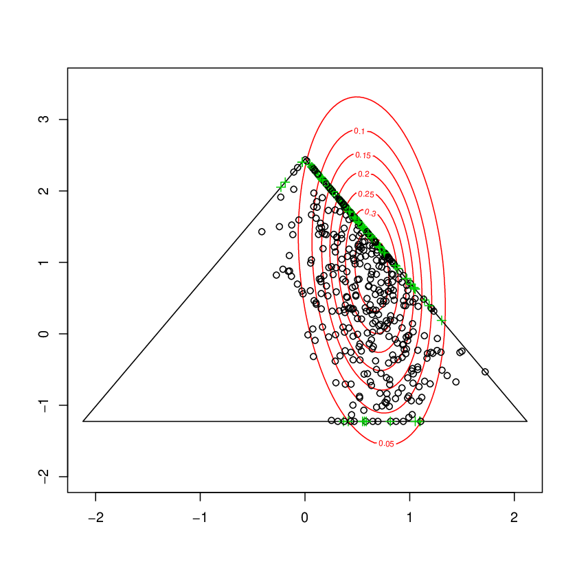
A key thing we have to mention about Figure 2 is that the contour lines look vertical but have in fact a negative slope. This is not seen because of the scaling of the ternary plot. The range of values of the x-axis is larger than the range of the simulated values in the first variable and thus the contour lines do not depict the negative slope they should.

4.2 Example 2. Time budget data

We will illustrate the performance of the zero–censored model using real data (6). There are $28$ individuals and for each person information about the time allocation in $10$ activities is known. The individuals are identified according to gender, country where they live, professional activity, and matrimonial status. We are not interested in their categorization but in the amount of time each person spent on $10$ categories of activities over $100$ days (the total is $100\times 24=2400$ hours fixed for every row) in $1976$ . The special feature of these data is that they contain some zero values. Some activities have zero allocation, for instance one woman did not spend even an hour on transportation linked to professional activity and four women did not spend any hour on occupation linked to children. This means that we have five compositions which have one zero in one component only.

The estimated parameters are

	$\displaystyle\hat{\bm{\mu}}=\left(1.075,-0.030,0.860,0.3830.367,0.222,-2.417,0.568,-0.465\right)\ \ \text{and}$

	$\displaystyle\hat{\bm{\Sigma}}=\left[\begin{array}[]{ccccccccc}0.289&0.574&0.109&0.076&0.019&0.035&0.038&0.008&0.030\\ 0.574&1.240&0.200&0.119&0.020&0.063&0.069&-0.020&0.002\\ 0.109&0.200&0.050&0.035&0.013&0.020&0.019&0.015&0.019\\ 0.076&0.119&0.035&0.037&0.013&0.009&0.013&0.015&0.027\\ 0.019&0.020&0.013&0.013&0.008&0.007&0.008&0.010&0.014\\ 0.035&0.063&0.020&0.009&0.007&0.020&0.018&0.010&0.010\\ 0.038&0.069&0.019&0.013&0.008&0.018&0.021&0.005&0.019\\ 0.008&-0.020&0.015&0.015&0.010&0.010&0.005&0.029&0.003\\ 0.030&0.002&0.019&0.027&0.014&0.010&0.019&0.003&0.079\\ \end{array}\right].$

4.3 Diagnostics for the zero–censored model

We have performed a similar goodness of fit diagnostic to the one 4 performed. We generated data from the fitted multivariate normal model and estimated the number of zeros in each component. For the first example with the simulated data we had $197$ out of $500$ vectors with one zero element, $171$ , $6$ and $20$ zeros in the first, second and third component respectively. The corresponding percentages are $\left(0.342,0.012,0.040\right)$ . We estimated the percentages of the zero values in each component to be $\left(0.347,0.008,0.040\right)$ respectively based on $10,000,000$ simulated observations. We repeated the same procedure for the real data in the second example and the results are presented in Table 1.

Table 1: Observed and estimated number of zeros for every component

Components	prof	tran	hous	kids	shop	pers	eat	slee	tele	leis
Observed
number of zeros	0	1	0	4	0	0	0	0	0	0
Estimated
number of zeros	0.593	0.547	2.106	2.151	0.002	0.000	0.000	0.000	0.137	0.000

From Table 1 we see that there is evidence to support the hypothesis that the fit of the model is not to be rejected. We could also use the $\chi^{2}$ test statistic as a discrepancy measure between the estimated and the observed frequencies and a $p$ –value could be calculated via simulations or via the $\chi^{2}$ distribution.

5 Conclusions

We developed a parametric zero-censored model for compositional data with zero values. The use of another multivariate model, such as the multivariate skew normal distribution (3) could also be utilized but the difficulty with this distribution is that more parameters need to be estimated, thus making the estimation procedure more difficult. This of course does not exclude the possibility of using this model.

The zero–censored model attacks the problem of zeros from a different perspective than the one 4 suggested. The data are projected on to the faces of the simplex using a non-orthogonal $1:1$ projection in contrast to the orthogonal 4 proposed. The advantage over Butler and Glasbey’s approach is that it is not difficult to project the data onto the edges regardless of the dimension. Both models however share the same problem, that of estimating the parameters of the normal distribution which becomes harder as the dimension increases. Both the zero-censored model (15) and the Butler and Glasbey’s model avoid the use of the log–ratio methodology or imputation of the zero values. A limitation of the zero-censored model is that it only allows for one zero per compositional vector. For instance if we have $D=3$ or $D=10$ components, only one zero should be present in each vector.

A further question when modelling compositional data by using either the proposed zero–censored model or the 4 model, is how to include covariates. 13 defined an alternative model based on the Kent distribution which offers the possibility for regression and handling zeros conveniently, at the cost of computational complexity.

References

Aitchison (1982) J. Aitchison The statistical analysis of compositional data. Journal of the Royal Statistical Society. Series B 44 (2), pp. 139–177. Cited by: §1.
Aitchison (2003) J. Aitchison The statistical analysis of compositional data. Reprinted by The Blackburn Press. Cited by: §1, §2.
Azzalini and Valle (1996) A. Azzalini and A.D. Valle The multivariate skew-normal distribution. Biometrika 83 (4), pp. 715. Cited by: §5.
Butler and Glasbey (2008) A. Butler and C. Glasbey A latent gaussian model for compositional data with zeros. Journal of the Royal Statistical Society: Series C (Applied Statistics) 57 (5), pp. 505–520. Cited by: §1, §1, §3, §3, §4.3, §5, §5, Modelling structural zeros in compositional data via a zero–censored multivariate normal model.
Dryden and Mardia (1998) I.L. Dryden and K.V. Mardia Statistical shape analysis. Vol. 4, Chichester: John Wiley & Sons. Cited by: footnote 1.
Härdle and Hlávka (2007) W. Härdle and Z. Hlávka Multivariate statistics: exercises and solutions. Springer Publishing Company, Incorporated. Cited by: §4.2.
Lancaster (1965) H.O. Lancaster The helmert matrices. American Mathematical Monthly 72 (1), pp. 4–12. Cited by: §2.
Le and Small (1999) H. Le and C.G. Small Multidimensional scaling of simplex shapes. Pattern Recognition 32 (9), pp. 1601–1613. Cited by: footnote 1.
Mardia et al. (1979) K.V. Mardia, J.T. Kent, and J.M. Bibby Multivariate Analysis. London: Academic Press. Cited by: §3.2.
Palarea Albaladejo et al. (2005) J. Palarea Albaladejo, M. Fernández, J. Antoni, and J. Gómez García Alr approach for replacing values below the detection limit. In Proceedings of the 2rd Compositional Data Analysis Workshop, Girona, Spain, Cited by: §1.
Palarea-Albaladejo et al. (2007) J. Palarea-Albaladejo, J.A. Martín-Fernández, and J. Gómez-García A parametric approach for dealing with compositional rounded zeros. Mathematical Geology 39 (7), pp. 625–645. Cited by: §1.
Scealy and Welsh (2011a) J.L. Scealy and A.H. Welsh Properties of a square root transformation regression model. In Proceedings of the 4rth Compositional Data Analysis Workshop, Girona, Spain, Cited by: §1.
Scealy and Welsh (2011b) J.L. Scealy and A.H. Welsh Regression for compositional data by using distributions defined on the hypersphere. Journal of the Royal Statistical Society. Series B 73 (3), pp. 351–375. Cited by: §5.
Strang (1988) G. Strang Linear algebra and its applications. Thomson Learning Inc.. Cited by: §3.
Tsagris and Stewart (2020) M. Tsagris and C. Stewart A folded model for compositional data analysis. Australian & New Zealand Journal of Statistics 62 (2), pp. 249–277. Cited by: §1, §1, §4.1.
Tsagris et al. (2011) M.T. Tsagris, S. Preston, and A.T.A. Wood A data-based power transformation for compositional data. In Proceedings of the 4rth Compositional Data Analysis Workshop, Girona, Spain, Cited by: §2.

Modelling structural zeros in compositional data via a zero–censored multivariate normal model

1 Introduction

2 The α\alpha–transformation

3 The zero–censored model

3.1 Gram–Schmidt orthonormalization process

3.2 The log–likelihood of the zero–censored model

3.3 Maximum likelihood estimation using the EM algorithm

3.4 E–step

Interior points.

Censored points.

3.5 M–step

3.6 Random values generation

Proposition 1.

Proof.

Proposition 2.

Proof.

4 Simulations

4.1 Example 1. Simulated data

4.2 Example 2. Time budget data

4.3 Diagnostics for the zero–censored model

5 Conclusions

References

2 The $\alpha$ –transformation