跳到论文正文
W Papers独立论文阅读器 arXiv:2208.12522 论文正文 计算阅读时间 · 0%
引用这篇论文根据当前论文元数据生成,正式投稿前建议核对。


License: CC BY 4.0
arXiv:2208.12522v1 [math.NA] 26 Aug 2022

Splitting Method for Support Vector Machine with Lower Semi-continuous Loss

Mingyu Mo, Qi Ye∗\text{{Ye}}^{*}

Abstract: In this paper, we study the splitting method based on alternating direction method of multipliers for support vector machine in reproducing kernel Hilbert space with lower semi-continuous loss function. If the loss function is lower semi-continuous and subanalytic, we use the Kurdyka-Lojasiewicz inequality to show that the iterative sequence induced by the splitting method globally converges to a stationary point. The numerical experiments also demonstrate the effectiveness of the splitting method.


Keywords: support vector machine, lower semi-continuous loss function, reproducing kernel Hilbert space, splitting method, Kurdyka-Lojasiewicz inequality.

Mathematics Subject Classification: 68Q32, 49J52.


1 Introduction

Support vector machine (SVM) is a well-known model for binary classification in machine learning. The basic idea of SVM is to find a function in a kernel-based function space to achieve the smallest regularized empirical risk such that the classification rule is constructed by the decision function and the sign function. The SVM is already achieved in reproducing kernel Hilbert spaces (RKHS) and convex loss functions (See [24]). After the success of the SVM in the RKHS with the convex loss functions, people continue to investigate whether the SVM in the RKHS can be feasible for nonconvex loss functions. Recently, different nonconvex loss functions are proposed and used for traditional SVM (see [6, 9, 15, 18, 19, 22, 29]). But the algorithms of the SVM in the RKHS with the general nonconvex loss function are still lack of study. If the loss function is convex, then it is lower semi-continuous (L.S.C.) while the lower semi-continuity can not imply the convexity. Moreover, the SVM in the RKHS with the L.S.C. and nonconvex loss functions can perform better than the convex loss functions in manny cases (see Section 5). Currently, people are most interested in the infinite-dimensional spaces for applications of machine learning such that the learning algorithm can be chosen from the enough large amounts of suitable solutions. In this paper, we consider the SVM in the infinite-dimensional RKHS with the L.S.C. loss function (See Section 2).

To construct the SVM in the RKHS, we will find a minimizer from Optimization (2.1). In this paper, we show that Optimization (2.1) has a minimizer in a finite-dimensional space spanned by the reproducing kernel basis related to the training data points. Thus Optimization (2.1) can be equivalently transferred to a finite-dimensional Optimization. Based the equivalent Optimization, we discuss the splitting method for Optimization (2.1) based on alternating direction method of multipliers (ADMM). By the splitting method, we obtain two subproblems which are computable easily. Moreover, the convergence of ADMM is already guaranteed well for the convex Optimizations (see [5]) and some special nonconvex Optimizations by the Kurdyka-Lojasiewicz (KL) property (see [11, 14]). To complete the proof, we reexchange the convergence theorems in [11, 14] and verify the convergence of the splitting method for Optimization (2.1) if the loss function is L.S.C. and subanalytic for the global convergence to a stationary point and the error bound.

This paper is organized as follows. We introduce the notations and preliminary materials of the SVM in Section 2. Next, we study the representer theorem for the L.S.C. loss functions and discuss how to solve Optimization (2.1) by the splitting method in Section 3. Moreover, we discuss the global convergence and convergent rates of splitting method for L.S.C. and subanalytic loss function in Section 4. Finally, we look at the numerical examples of the different loss functions and RKHSs for the synthetic data and the real data in Section 5.

2 Notations and Preliminaries

In this section, we review some notations and preliminaries of SVM. We denote the set of positive integers as ℕ\mathbb{N} and the dd-dimensional Euclidean space as ℝd\mathbb{R}^{d} respectively. For the sample space X⊆ℝdX\subseteq\mathbb{R}^{d} and the label space Y={+1,−1}Y=\{+1,-1\}, the training data D:={(𝒙i,yi):i=1,2,…,N}D:=\{(\boldsymbol{x}_{i},y_{i}):i=1,2,...,N\} is composed of input data 𝒙1,𝒙2,…,𝒙N∈X\boldsymbol{x}_{1},\boldsymbol{x}_{2},...,\boldsymbol{x}_{N}\in X and output data y1,y2,…,yN∈Yy_{1},y_{2},...,y_{N}\in Y. We will find a mapping ℛ:X→Y\mathcal{R}:X\to Y related to DD such that ℛ⁡(𝒙)\mathcal{R}(\boldsymbol{x}) is a good approximation of the response yy to an arbitrary 𝒙\boldsymbol{x}. For the rest of this paper, the symbol 𝒙\boldsymbol{x} always refers to column vector, so 𝒙T\boldsymbol{x}^{T} denotes row vector.

The SVM is an important class of mappings ℛ:X→Y\mathcal{R}:X\to Y. The basic idea of traditional SVM is to find a hyperplane in XX that classifies all the training data in DD correctly and creates the biggest margin. Thus we construct ℛ:X→Y\mathcal{R}:X\to Y by the hyperplane and the sign function. However, the hyperplane to separate DD may not exist and we can only accept the hyperplane that misclassifies some training data. To help us define what we mean by ”good”, we introduce the loss function of the SVM to find the hyperplane and its equivalent optimization is a optimization with an offset term in a RKHS consisting all linear functions on XX with the linear reproducing kernel (See [24, 1.3 History of SVMs and Geometrical Interpretation]). Obviously, the RKHS is a finite-dimensional kernel-based function space which is isometrically isomorphic to ℝd\mathbb{R}^{d}. Generally speaking, the SVM is to find a function on XX that achieves the smallest regularized empirical risk in a given RKHS such that the classification rule ℛ:X→Y\mathcal{R}:X\to Y is constructed by the decision function and the sign function.

Since the RKHS is only a finite-dimensional space, in the rest of this paper, we shall discuss the SVM in some special infinite-dimensional spaces with different kinds of kernels. Generally speaking, a Hilbert space ℋ\mathcal{H} of functions f:X→ℝf:X\rightarrow\mathbb{R} equipped with the complete inner product ⟨⋅,⋅⟩ℋ\langle\cdot,\cdot\rangle_{\mathcal{H}} and the reproducing kernel K:X×X→ℝK:X\times X\rightarrow\mathbb{R} is called an RKHS if it satisfies the following two conditions

(i) K⁡(𝒙,⋅)∈ℋK(\boldsymbol{x},\cdot)\in\mathcal{H} for all 𝒙∈X\boldsymbol{x}\in X,

(ii) f⁡(𝒙)=⟨f,K⁡(𝒙,⋅)⟩ℋf(\boldsymbol{x})=\langle f,K(\boldsymbol{x},\cdot)\rangle_{\mathcal{H}} for all f∈ℋf\in\mathcal{H} and all 𝒙∈X\boldsymbol{x}\in X.

In particular, for any f,g∈ℋf,g\in\mathcal{H}, the corresponding norm ‖f‖ℋ=⟨f,f⟩ℋ\|f\|_{\mathcal{H}}=\sqrt{\langle f,f\rangle_{\mathcal{H}}} and the corresponding metric ‖f−g‖ℋ\|f-g\|_{\mathcal{H}} are complete. On the other hand, the reproducing kernel KK of an RKHS ℋ\mathcal{H} is uniquely determined. By [26, Theorem 10.3 and 10.4], KK is symmetric and positive definite (see [24, Definition 4.15]). In some cases, KK can be symmetric and strictly positive definite, for instance, Gaussian kernels, Matérn kernels and so on. In particular, the value K⁡(𝒙,𝒙′)K(\boldsymbol{x},\boldsymbol{x}^{\prime}) can often be interpreted as a measure of dissimilarity between the input values 𝒙\boldsymbol{x} and 𝒙′\boldsymbol{x}^{\prime}.

For more flexible kernels such as those of Gaussian kernels, which belong to the most important kernels in practice, the offset term has neither a known theoretical nor an empirical advantage. In addition, the theoretical analysis is often substantially complicated by offset term. Thus, we decide to exclusively consider the SVM in the RKHS without an offset term. Let us fix such an RKHS ℋ\mathcal{H} and a real number λ>0\lambda>0, the SVM in the RKHS finds a minimizer of

inff∈ℋ1N​∑i=1NL⁡(𝒙i,yi,f⁡(𝒙i))+λ​‖f‖ℋ2.\inf_{f\in\mathcal{H}}\ \frac{1}{N}\sum_{i=1}^{N}L(\boldsymbol{x}_{i},y_{i},f(\boldsymbol{x}_{i}))+\lambda\|f\|_{\mathcal{H}}^{2}. (2.1)

where L:X×Y×ℝ→[0,∞)L:X\times Y\times\mathbb{R}\rightarrow[0,\infty) is a loss function and λ​‖f‖ℋ2\lambda\|f\|_{\mathcal{H}}^{2} is the regularization term used to penalize ff with the large RKHS norm. In the following, we will interpret L⁡(𝒙,y,f⁡(𝒙))L(\boldsymbol{x},y,f(\boldsymbol{x})) as the loss of predicting yy by f⁡(𝒙)f(\boldsymbol{x}) if 𝒙\boldsymbol{x} is observed, that is, the smaller the value L⁡(𝒙,y,f⁡(𝒙))L(\boldsymbol{x},y,f(\boldsymbol{x})) is, the better f⁡(𝒙)f(\boldsymbol{x}) predicts yy in the sense of LL. We denote the minimizer of Optimization (2.1) as fDf_{D}. Next we use fDf_{D} to construct the SVM in the RKHS as follows.

ℛ⁡(𝒙)={+1,fD​(𝒙)≥0,−1,fD​(𝒙)<0.\mathcal{R}(\boldsymbol{x})=\begin{cases}+1,&f_{D}(\boldsymbol{x})\geq 0,\\ -1,&f_{D}(\boldsymbol{x})<0.\end{cases} (2.2)

Moreover, the classification rules constructed by different minimizers of Optimization (2.1) have no difference in performance. In conclusion, we just need to find a minimizer of Optimization (2.1). Next we discuss the solution of Optimization (2.1) and splitting method for Optimization (2.1) in Section 3.

3 Representer Theorem and Splitting Method

In this section, we discuss how to solve Optimization (2.1) by splitting method. First we discuss the solution of Optimization (2.1). The loss function is the key factor of the SVM in the RKHS, because it not only determines the sensitivity to the noise of training data but also affects the sparsity of the SVM in the RKHS. For binary classification, the most straightforward loss function is the 0-1 loss function, which is an ”ideal” loss function (see [7]). However, 0-1 loss function is bounded, nonconvex and L.S.C. but discontinuous. Trying to optimize 0-1 loss function directly leads to a L.S.C. and nonconvex optimization problem which is unable to deal with by traditional optimization theory and algorithm. Therefore, a number of surrogate loss functions are proposed in the literature, such as convex loss function, that is, L(𝒙,y,⋅)L(\boldsymbol{x},y,\cdot) is a convex function for all 𝒙∈X\boldsymbol{x}\in X and y∈Yy\in Y. Besides convexity, we can define other loss functions in a similar way, such as continuity, smoothness, lower semi-continuity, etc. Specially, if LL is convex, then LL is L.S.C. But the lower semi-continuity can not imply the convexity.

Generally speaking, loss functions can be divided into two categories: convex loss functions and nonconvex loss functions. Convex loss functions including Hinge loss, square loss are the most commonly used. If LL is a convex loss function, then the classical representer theorem [24, Theorem 5.5] assures that Optimization (2.1) has a unique minimizer fDf_{D} such that

fD∈span⁡{K⁡(𝒙1,⋅),…,K⁡(𝒙N,⋅)},f_{D}\in\mathrm{span}\{K(\boldsymbol{x}_{1},\cdot),...,K(\boldsymbol{x}_{N},\cdot)\},

where span​{K⁡(𝒙1,⋅),…,K⁡(𝒙N,⋅)}\text{{span}}\{K(\boldsymbol{x}_{1},\cdot),...,K(\boldsymbol{x}_{N},\cdot)\} denotes the set of all finite linear combinations of {K⁡(𝒙1,⋅),…,K⁡(𝒙N,⋅)}\{K(\boldsymbol{x}_{1},\cdot),...,K(\boldsymbol{x}_{N},\cdot)\}. A remarkable consequence of the representation above is the fact that fDf_{D} is contained in a known finite- dimensional space, even if the space ℋ\mathcal{H} itself is substantially larger. Thus, the convex loss functions are viewed as highly preferable in many publications because of their computational advantages (unique minimizer, ease-of-use, ability to be efficiently optimized by convex optimization tools, etc.).

However, the convexity also offer poor approximations to 0-1 loss function. Therefore, different nonconvex loss functions, such as ramp loss, truncated logistic loss, truncated least square loss, truncated least square loss, bi-truncated loss, generalized exponential loss, generalized logistic loss and Sigmoid loss are proposed and used in SVM (see [6, 9, 15, 18, 19, 22, 29]). These loss functions mentioned above and 0-1 loss functions are L.S.C. and nonconvex. Recently, [12, Corollary 4.1] generalizes the classical representer theorem to the L.S.C. loss function. Moreover, by the preliminary numerical experiments, we find that the SVM in the RKHS with the L.S.C. and nonconvex loss functions may be better than the convex loss functions (see Section 5). Thus, we will discuss the SVM in the RKHS with the L.S.C. loss functions. Before we show our main result, we need some concepts and properties of ℋ\mathcal{H}.

From [27, Definition 2.1], an RKHS ℋ\mathcal{H} can be seen as the two-sided reproducing kernel Banach space. On the other hand, the Riesz Representation Theorem assures that the dual space of ℋ′\mathcal{H}^{{}^{\prime}} is isometrically isomorphic to ℋ\mathcal{H}, that is, ℋ′≅ℋ\mathcal{H}^{{}^{\prime}}\cong\mathcal{H}, which ensures that ℋ\mathcal{H} is reflexive. Hence, by [8, Definition 2.2.27] and reflexity of ℋ\mathcal{H}, it shows that the predual space of ℋ\mathcal{H} is ℋ′\mathcal{H}^{{}^{\prime}}. Moreover, since ℋ\mathcal{H} is also strictly convex and smooth, we obtain the following formula of Fréchet derivative (see [27, Remark 2.24])

∇(∥⋅∥ℋ)(f)=f‖f‖ℋ∈ℋ,∀f≠0,\nabla(\|\cdot\|_{\mathcal{H}})(f)=\frac{f}{\|f\|_{\mathcal{H}}}\in\mathcal{H},\ \ \forall f\neq 0, (3.1)

where ∇\nabla denotes the Fréchet derivative. In particular, for a differentiable real function, ∇\nabla represents the gradient.

Proposition 3.1.

If LL is lower semi-continuous, then Optimization (2.1) has a minimizer fDf_{D} such that

fD∈span⁡{K⁡(𝒙1,⋅),…,K⁡(𝒙N,⋅)}.f_{D}\in\mathrm{span}\{K(\boldsymbol{x}_{1},\cdot),...,K(\boldsymbol{x}_{N},\cdot)\}.
Proof.

Since ℋ\mathcal{H} is an reproducing kernel Banach space which has a predual space ℋ′\mathcal{H}^{{}^{\prime}}, from the condition (i) in the definition of the RKHS, we have that

{K(𝒙,⋅):𝒙∈X}⊆ℋ≅ℋ′.\{K(\boldsymbol{x},\cdot):\boldsymbol{x}\in X\}\subseteq\mathcal{H}\cong\mathcal{H}^{{}^{\prime}}.

Therefore, [12, Corollary 4.1] ensures that Optimization (2.1) has a minimizer fDf_{D} such that

∇(∥⋅∥ℋ)(fD)∈span{K(𝒙1,⋅),…,K(𝒙N,⋅)}.\nabla(\|\cdot\|_{\mathcal{H}})(f_{D})\in\text{{span}}\{K(\boldsymbol{x}_{1},\cdot),...,K(\boldsymbol{x}_{N},\cdot)\}.

If fD≠0f_{D}\neq 0, then (3.1) shows that

fD‖fD‖ℋ∈span​{K⁡(𝒙1,⋅),…,K⁡(𝒙N,⋅)}.\frac{f_{D}}{\|f_{D}\|_{\mathcal{H}}}\in\text{{span}}\{K(\boldsymbol{x}_{1},\cdot),...,K(\boldsymbol{x}_{N},\cdot)\}.

Moreover, by the definition of span​{K⁡(𝒙1,⋅),…,K⁡(𝒙N,⋅)}\text{{span}}\{K(\boldsymbol{x}_{1},\cdot),...,K(\boldsymbol{x}_{N},\cdot)\}, we have that

fD∈span​{K⁡(𝒙1,⋅),…,K⁡(𝒙N,⋅)}.f_{D}\in\text{{span}}\{K(\boldsymbol{x}_{1},\cdot),...,K(\boldsymbol{x}_{N},\cdot)\}.

If fD=0f_{D}=0, then 0∈span​{K⁡(𝒙1,⋅),…,K⁡(𝒙N,⋅)}0\in\text{{span}}\{K(\boldsymbol{x}_{1},\cdot),...,K(\boldsymbol{x}_{N},\cdot)\}. In conclusion,

fD∈span​{K⁡(𝒙1,⋅),…,K⁡(𝒙N,⋅)}.f_{D}\in\text{{span}}\{K(\boldsymbol{x}_{1},\cdot),...,K(\boldsymbol{x}_{N},\cdot)\}.

The proof is complete. ∎

Remark 3.2.

If LL is L.S.C. and nonconvex, then Optimization (2.1) may have more than one minimizers. Moreover, Proposition 3.1 guarantees that at least one of minimizers is contained in span​{K⁡(𝒙1,⋅),…,K⁡(𝒙N,⋅)}\text{{span}}\{K(\boldsymbol{x}_{1},\cdot),...,K(\boldsymbol{x}_{N},\cdot)\}. Thus, we focus on find the minimizer in span​{K⁡(𝒙1,⋅),…,K⁡(𝒙N,⋅)}\text{{span}}\{K(\boldsymbol{x}_{1},\cdot),...,K(\boldsymbol{x}_{N},\cdot)\}.

By Proposition 3.1, Optimization (2.1) in the RKHS ℋ\mathcal{H} can be equivalently transferred to Optimization (2.1) in span⁡{K⁡(𝒙1,⋅),…,K⁡(𝒙N,⋅)}\mathrm{span}\{K(\boldsymbol{x}_{1},\cdot),...,K(\boldsymbol{x}_{N},\cdot)\}. Next we show that Optimization (2.1) in span⁡{K⁡(𝒙1,⋅),…,K⁡(𝒙N,⋅)}\mathrm{span}\{K(\boldsymbol{x}_{1},\cdot),...,K(\boldsymbol{x}_{N},\cdot)\} also can be equivalently transferred to a finite-dimensional Optimization in ℝN\mathbb{R}^{N}. We denote the kernel matrix of KK as

A:=(K⁡(𝒙i,𝒙j))i,j=1N,N,A:=\left(K(\boldsymbol{x}_{i},\boldsymbol{x}_{j})\right)_{i,j=1}^{N,N},

and AA is symmetric and positive definite. For each f∈span​{K⁡(𝒙1,⋅),…,K⁡(𝒙N,⋅)}f\in\text{{span}}\{K(\boldsymbol{x}_{1},\cdot),...,K(\boldsymbol{x}_{N},\cdot)\}, there exists a unique vector 𝒄=(c1,…,cN)T∈ℝN\boldsymbol{c}=(c_{1},...,c_{N})^{T}\in\mathbb{R}^{N} such that ff has the finite representation

f=∑j=1Ncj​K​(𝒙j,⋅),f=\sum_{j=1}^{N}c_{j}K(\boldsymbol{x}_{j},\cdot),

which ensures that

f⁡(𝒙i)=∑j=1Ncj​K​(𝒙j,𝒙i)=∑j=1NK⁡(𝒙i,𝒙j)​cj=(A​𝒄)i.f(\boldsymbol{x}_{i})=\sum_{j=1}^{N}c_{j}K(\boldsymbol{x}_{j},\boldsymbol{x}_{i})=\sum_{j=1}^{N}K(\boldsymbol{x}_{i},\boldsymbol{x}_{j})c_{j}=(A\boldsymbol{c})_{i}.

Therefore, it is easy to check that

f↦(f⁡(𝒙1),f⁡(𝒙2),…,f⁡(𝒙N))T=A​𝒄f\mapsto(f(\boldsymbol{x}_{1}),f(\boldsymbol{x}_{2}),...,f(\boldsymbol{x}_{N}))^{T}=A\boldsymbol{c} (3.2)

is an isometric isomorphism from span⁡{K⁡(𝒙1,⋅),…,K⁡(𝒙N,⋅)}\mathrm{span}\{K(\boldsymbol{x}_{1},\cdot),...,K(\boldsymbol{x}_{N},\cdot)\} onto ℝN\mathbb{R}^{N}. On the other hand, combining the property of inner product ⟨⋅,⋅⟩ℋ\langle\cdot,\cdot\rangle_{\mathcal{H}} with the reproducing property in the RKHS, it holds that

‖f‖ℋ2=⟨f,∑i=1Nci​K​(𝒙i,⋅)⟩ℋ=∑i=1Nci​⟨f,K⁡(𝒙i,⋅)⟩ℋ=∑i=1Nci​f​(𝒙i)=𝒄T​A​𝒄.\|f\|_{\mathcal{H}}^{2}=\langle f,\sum_{i=1}^{N}c_{i}K(\boldsymbol{x}_{i},\cdot)\rangle_{\mathcal{H}}=\sum_{i=1}^{N}c_{i}\langle f,K(\boldsymbol{x}_{i},\cdot)\rangle_{\mathcal{H}}=\sum_{i=1}^{N}c_{i}f(\boldsymbol{x}_{i})=\boldsymbol{c}^{T}A\boldsymbol{c}. (3.3)

So Optimization (2.1) can be equivalently transferred to the following Optimization in ℝN\mathbb{R}^{N}

min𝒄∈ℝN⁡1N​∑i=1NL⁡(𝒙i,yi,(A​𝒄)i)+λ​𝒄T​A​𝒄,\min_{\boldsymbol{c}\in\mathbb{R}^{N}}\hskip 4.25006pt\frac{1}{N}\sum_{i=1}^{N}L(\boldsymbol{x}_{i},y_{i},(A\boldsymbol{c})_{i})+\lambda\boldsymbol{c}^{T}A\boldsymbol{c}, (3.4)

We denote the minimizer of Optimization (3.4) as 𝒄D=((c1)D,(c2)D,…,(cN)D)T\boldsymbol{c}_{D}=((c_{1})_{D},(c_{2})_{D},...,(c_{N})_{D})^{T}, it follows that

fD=∑i=1N(ci)D​K​(𝒙i,⋅).f_{D}=\sum_{i=1}^{N}(c_{i})_{D}K(\boldsymbol{x}_{i},\cdot).

This ensures that we employ the finite suitable parameters to reconstruct the SVM in the RKHS.

By this idea, we consider to find an algorithm based on Optimization (3.4) to compute Optimization (2.1) easily. At present, we mainly use the subdifferential, proximal operator and Fenchel conjugate of loss function to design algorithms for SVM, such as subgradient method, Lagrange multipliers method and sequential minimal optimization (SMO). These classical numerical algorithms are suitable for solving convex and smooth programs. Since 𝒄↦(A​𝒄)i\boldsymbol{c}\mapsto(A\boldsymbol{c})_{i} is continuous, the lower semi-continuity of L(𝒙i,yi,⋅)L(\boldsymbol{x}_{i},y_{i},\cdot) guarantees the lower semi-continuity of 𝒄↦L⁡(𝒙i,yi,(A​𝒄)i)\boldsymbol{c}\mapsto L(\boldsymbol{x}_{i},y_{i},(A\boldsymbol{c})_{i}) for all i=1,2,…,Ni=1,2,...,N which ensures that FF is L.S.C.. On the other hand, it is clear that GG is continuous. In conclusion, Optimization (3.4) is L.S.C. finite-dimensional Optimization which may be nonsmooth or nonconvex. Many classical numerical algorithms are not suitable for Optimization (3.4) when LL is L.S.C.

The ADMM algorithm, as one of splitting techniques, has been successfully exploited in a wide range of structured regularization optimization problems in machine learning. ADMM can even be used to minimize nonsmooth or nonconvex function, which solves optimization problem by breaking them into smaller pieces. Moreover, Paper [25] discusses how to use ADMM for the traditional SVM with the 0-1 loss function. For the general L.S.C. functions and kernels, we observe that the subproblems in ADMM for Optimization (3.4) can be transferred into some Optimizations in ℝ\mathbb{R} and a well-posed linear system, each of which are thus easier to handle. In summary, we discuss the splitting method based on ADMM for Optimization (2.1). Moreover, if the sample size NN is small to moderate, then the preliminary numerical experiments show that the splitting method is a fast algorithm for Optimization (2.1) (see Section 5). Hence, we will study how to solve Optimization (2.1) by the splitting method. For notational convenience, let

F⁡(A​𝒄)=1N​∑i=1NL⁡(𝒙i,yi,(A​𝒄)i),G⁡(𝒄)=λ​𝒄T​A​𝒄.F(A\boldsymbol{c})=\frac{1}{N}\sum\limits_{i=1}^{N}L(\boldsymbol{x}_{i},y_{i},(A\boldsymbol{c})_{i}),\ \ G(\boldsymbol{c})=\lambda\boldsymbol{c}^{T}A\boldsymbol{c}.

To describe the algorithm, we first reformulate Optimization (3.4) as

min𝒂,𝒄F⁡(𝜶)+G⁡(𝒄),s.t.𝜶=A​𝒄.\begin{array}[]{cl}\displaystyle\min_{\boldsymbol{a},\boldsymbol{c}}&\displaystyle F(\boldsymbol{\alpha})+G(\boldsymbol{c}),\\ \text{s.t.}&\boldsymbol{\alpha}=A\boldsymbol{c}.\end{array} (3.5)

Recall that the augmented Lagrangian function is defined as:

ℒρ​(𝜶,𝒄,𝜸)=F⁡(𝜶)+G⁡(𝒄)+𝜸T​(𝜶−A​𝒄)+ρ2​‖𝜶−A​𝒄‖2,\mathcal{L}_{\rho}(\boldsymbol{\alpha},\boldsymbol{c},\boldsymbol{\gamma})=F(\boldsymbol{\alpha})+G(\boldsymbol{c})+\boldsymbol{\gamma}^{T}(\boldsymbol{\alpha}-A\boldsymbol{c})+\frac{\rho}{2}\|\boldsymbol{\alpha}-A\boldsymbol{c}\|^{2},

where the Lagrangian multiplier ρ>0\rho>0 and ∥⋅∥\|\cdot\| denotes 22-norm in Euclidean space. The splitting method is presented as follows. Suppose that the algorithm is initialized at (𝜶0,𝒄0,𝜸0)(\boldsymbol{\alpha}^{0},\boldsymbol{c}^{0},\boldsymbol{\gamma}^{0}), its iterative scheme is

𝜶k+1\displaystyle\boldsymbol{\alpha}^{k+1} ∈argmin𝜶∈ℝNℒρ​(𝜶,𝒄k,𝜸k),\displaystyle\in\mathop{\mathrm{argmin}}_{\boldsymbol{\alpha}\in\mathbb{R}^{N}}\ \mathcal{L}_{\rho}(\boldsymbol{\alpha},\boldsymbol{c}^{k},\boldsymbol{\gamma}^{k}), (S-1)
𝒄k+1\displaystyle\boldsymbol{c}^{k+1} ∈argmin𝒄∈ℝNℒρ​(𝜶k+1,𝒄,𝜸k),\displaystyle\in\mathop{\mathrm{argmin}}_{\boldsymbol{c}\in\mathbb{R}^{N}}\ \mathcal{L}_{\rho}(\boldsymbol{\alpha}^{k+1},\boldsymbol{c},\boldsymbol{\gamma}^{k}), (S-2)
𝜸k+1\displaystyle\boldsymbol{\gamma}^{k+1} :=𝜸k+ρ⁡(𝜶k+1−A​𝒄k+1),\displaystyle:=\boldsymbol{\gamma}^{k}+\rho(\boldsymbol{\alpha}^{k+1}-A\boldsymbol{c}^{k+1}), (S-3)
sk+1\displaystyle s^{k+1} :=∑i=1N(𝒄k+1)i​K​(𝒙i,⋅),\displaystyle:=\sum_{i=1}^{N}(\boldsymbol{c}^{k+1})_{i}K(\boldsymbol{x}_{i},\cdot), (S-4)

where kk is an iteration counter. Since (S-1) only depends on 𝜶\boldsymbol{\alpha} and (S-2) only depends on 𝒄\boldsymbol{c}, by combining the linear and quadratic terms in ℒρ\mathcal{L}_{\rho}, we equivalently transfer (S-1) and (S-2) to

𝜶k+1\displaystyle\boldsymbol{\alpha}^{k+1} ∈argmin𝜶∈ℝNF⁡(𝜶)+ρ2​‖𝜶−A​𝒄k+1ρ​𝜸k‖2,\displaystyle\in\mathop{\mathrm{argmin}}_{\boldsymbol{\alpha}\in\mathbb{R}^{N}}\ F(\boldsymbol{\alpha})+\frac{\rho}{2}\|\boldsymbol{\alpha}-A\boldsymbol{c}^{k}+\frac{1}{\rho}\boldsymbol{\gamma}^{k}\|^{2}, (S-1’)
𝒄k+1\displaystyle\boldsymbol{c}^{k+1} ∈argmin𝒄∈ℝNG⁡(𝒄)+ρ2​‖𝜶k+1−A​𝒄+1ρ​𝜸k‖2.\displaystyle\in\mathop{\mathrm{argmin}}_{\boldsymbol{c}\in\mathbb{R}^{N}}\ G(\boldsymbol{c})+\frac{\rho}{2}\|\boldsymbol{\alpha}^{k+1}-A\boldsymbol{c}+\frac{1}{\rho}\boldsymbol{\gamma}^{k}\|^{2}. (S-2’)

By definition, it is easy to check that (S-1’) is L.S.C. and (S-2’) is continuous. Moreover, (S-1’) and (S-2’) is coercive (see [1, Definition 2.13]), that is,

lim‖𝜶‖→∞F⁡(𝜶)+ρ2​‖𝜶−A​𝒄k+1ρ​𝜸k‖2→∞,\displaystyle\lim_{\|\boldsymbol{\alpha}\|\rightarrow\infty}F(\boldsymbol{\alpha})+\frac{\rho}{2}\|\boldsymbol{\alpha}-A\boldsymbol{c}^{k}+\frac{1}{\rho}\boldsymbol{\gamma}^{k}\|^{2}\to\infty,
lim‖𝒄‖→∞G⁡(𝒄)+ρ2​‖𝜶k+1−A​𝒄+1ρ​𝜸k‖2→∞.\displaystyle\lim_{\|\boldsymbol{c}\|\rightarrow\infty}G(\boldsymbol{c})+\frac{\rho}{2}\|\boldsymbol{\alpha}^{k+1}-A\boldsymbol{c}+\frac{1}{\rho}\boldsymbol{\gamma}^{k}\|^{2}\to\infty.

Thus, Weierstrass Theorem [1, Theorem 2.14] assures that (S-1’) and (S-2’) both have a solution. As a consequence, the splitting method above is well-defined and an infinite iterative sequence {(𝜶k,𝒄k,𝜸k,sk)}\{(\boldsymbol{\alpha}^{k},\boldsymbol{c}^{k},\boldsymbol{\gamma}^{k},s^{k})\} is generated. Moreover, {sk}\{s^{k}\} can be seen as an infinite iterative sequence to approximate the minimizer of Optimization (2.1).

Next, we discuss how to solve subproblems (S-1’) and (S-2’). As for (S-1’), since FF and ∥⋅∥2\|\cdot\|^{2} can be split of the variable into subvectors, that is,

1N​∑i=1NL⁡(𝒙i,yi,αi)+ρ2​‖𝜶−A​𝒄k+1ρ​𝜸k‖2=∑i=1NL⁡(𝒙i,yi,αi)N+ρ2​(αi−(A​𝒄k)i+1ρ​(𝜸k)i)2,\frac{1}{N}\sum\limits_{i=1}^{N}L(\boldsymbol{x}_{i},y_{i},\alpha_{i})+\frac{\rho}{2}\|\boldsymbol{\alpha}-A\boldsymbol{c}^{k}+\frac{1}{\rho}\boldsymbol{\gamma}^{k}\|^{2}=\sum_{i=1}^{N}\frac{L(\boldsymbol{x}_{i},y_{i},\alpha_{i})}{N}+\frac{\rho}{2}\left(\alpha_{i}-(A\boldsymbol{c}^{k})_{i}+\frac{1}{\rho}(\boldsymbol{\gamma}^{k})_{i}\right)^{2},

we equivalently transfer an Optimization in ℝN\mathbb{R}^{N} to some Optimizations in ℝ\mathbb{R}, that is,

(𝜶k+1)i∈argminαiL⁡(𝒙i,yi,αi)N+ρ2(αi−(A𝒄k)i+1ρ(𝜸k)i)2,i=1,2,…,N.(\boldsymbol{\alpha}^{k+1})_{i}\in\mathop{\mathrm{argmin}}_{\alpha_{i}}\ \frac{L(\boldsymbol{x}_{i},y_{i},\alpha_{i})}{N}+\frac{\rho}{2}\left(\alpha_{i}-(A\boldsymbol{c}^{k})_{i}+\frac{1}{\rho}(\boldsymbol{\gamma}^{k})_{i}\right)^{2},\ i=1,2,...,N. (S-1”)

In other words, we solve (S-1’) in NN-dimensional space by breaking it into NN Optimizations (S-1”) in 1-dimensional space and each of them is easier to handle. To illustrate above, we give a simple example. Assume that LL is Hinge loss, that is,

LHinge​(𝒙i,yi,αi)=max⁡{0,1−yi​αi}.L_{\text{Hinge}}(\boldsymbol{x}_{i},y_{i},\alpha_{i})=\max\{0,1-y_{i}\alpha_{i}\}.

By simple algebra, if yi=+1y_{i}=+1, then

(𝜶k+1)i={ui+1ρ​Nui<1−1ρ​N,11−1ρ​N≤ui<1,uiui≥1,(\boldsymbol{\alpha}^{k+1})_{i}=\begin{cases}u_{i}+\frac{1}{\rho N}&u_{i}<1-\frac{1}{\rho N},\\ 1&1-\frac{1}{\rho N}\leq u_{i}<1,\\ u_{i}&u_{i}\geq 1,\end{cases}

where ui=(A​𝒄k)i−1ρ​(𝜸k)iu_{i}=(A\boldsymbol{c}^{k})_{i}-\frac{1}{\rho}(\boldsymbol{\gamma}^{k})_{i}. On the other hand, if yi=−1y_{i}=-1, then

(𝜶k+1)i={uiui<−1,−1−1≤ui<−1+1ρ​N,ui−1ρ​Nui≥−1+1ρ​N.(\boldsymbol{\alpha}^{k+1})_{i}=\begin{cases}u_{i}&u_{i}<-1,\\ -1&-1\leq u_{i}<-1+\frac{1}{\rho N},\\ u_{i}-\frac{1}{\rho N}&u_{i}\geq-1+\frac{1}{\rho N}.\end{cases}

For the general L.S.C. loss function LL, the solution set of (S-1”) may not be a singleton. For example, assume that LL is ramp loss, that is,

LRamp​(𝒙i,yi,αi)={11−yi​αi>1,1−yi​αi0<1−yi​αi≤1,01−yi​αi<0.L_{\text{Ramp}}(\boldsymbol{x}_{i},y_{i},\alpha_{i})=\begin{cases}1&1-y_{i}\alpha_{i}>1,\\ 1-y_{i}\alpha_{i}&0<1-y_{i}\alpha_{i}\leq 1,\\ 0&1-y_{i}\alpha_{i}<0.\end{cases}

Similarly, by simple algebra, if 0<1ρ​N<20<\frac{1}{\rho N}<2 and yi=+1y_{i}=+1, then

(𝜶k+1)i={uiui≤−12​ρ​N,ui​or​ui+1ρ​Nui=−12​ρ​N,ui+1ρ​N−12​ρ​N<ui≤1−1p​N,11−1ρ​N<ui<1,uiui≥1.(\boldsymbol{\alpha}^{k+1})_{i}=\begin{cases}u_{i}&u_{i}\leq-\frac{1}{2\rho N},\\ u_{i}\ \text{or}\ u_{i}+\frac{1}{\rho N}&u_{i}=-\frac{1}{2\rho N},\\ u_{i}+\frac{1}{\rho N}&-\frac{1}{2\rho N}<u_{i}\leq 1-\frac{1}{pN},\\ 1&1-\frac{1}{\rho N}<u_{i}<1,\\ u_{i}&u_{i}\geq 1.\end{cases}

if 0<1ρ​N<20<\frac{1}{\rho N}<2 and yi=−1y_{i}=-1, then

(𝜶k+1)i={uiui≤−1,−1−1<ui<−1+1ρ​N,ui−1ρ​N−1+1p​N≤ui<12​ρ​N,ui​or​ui−1ρ​Nui=12​ρ​N,uiui>12​ρ​N.(\boldsymbol{\alpha}^{k+1})_{i}=\begin{cases}u_{i}&u_{i}\leq-1,\\ -1&-1<u_{i}<-1+\frac{1}{\rho N},\\ u_{i}-\frac{1}{\rho N}&-1+\frac{1}{pN}\leq u_{i}<\frac{1}{2\rho N},\\ u_{i}\ \text{or}\ u_{i}-\frac{1}{\rho N}&u_{i}=\frac{1}{2\rho N},\\ u_{i}&u_{i}>\frac{1}{2\rho N}.\end{cases}

In this case, we choose one of the elements in the solution set as (𝜶k+1)i,i=1,…,N(\boldsymbol{\alpha}^{k+1})_{i},\ i=1,...,N.

As for (S-2’), since AA is symmetric and strictly positive definite and λ,ρ>0\lambda,\rho>0, it is clear that (S-2’) is nonnegative, convex and continuously differentiable. Moreover, 𝒄k+1\boldsymbol{c}^{k+1} is a minimizer of (S-2’) and thus a stationary point, that is,

2​λ​A​𝒄k+1−ρ​A​(𝜶k+1−A​𝒄k+1+1ρ​𝜸k)=0.2\lambda A\boldsymbol{c}^{k+1}-\rho A(\boldsymbol{\alpha}^{k+1}-A\boldsymbol{c}^{k+1}+\frac{1}{\rho}\boldsymbol{\gamma}^{k})=0.

By rearranging terms, 𝒄k+1\boldsymbol{c}^{k+1} is the solution of the following well-posed linear system

(2​λ​I+ρ​A)​𝒄=ρ​𝜶k+1+𝜸k.(2\lambda I+\rho A)\boldsymbol{c}=\rho\boldsymbol{\alpha}^{k+1}+\boldsymbol{\gamma}^{k}. (S-2”)

where II is the identity matrix with and order NN. Since 2​λ​I+ρ​A2\lambda I+\rho A is symmetric and strictly positive definite, we can use conjugate gradient method to obtain 𝒄k+1\boldsymbol{c}^{k+1} (See [13, 4.7.3 Conjugate Gradient Methods]).

When 𝜶k+1\boldsymbol{\alpha}^{k+1} and 𝒄k+1\boldsymbol{c}^{k+1} is acquired, we can obtain 𝜸k+1\boldsymbol{\gamma}^{k+1} by (S-3). However, we have a simpler one in mind that accomplishes the same goal. Substituting (S-3) into (S-2”) and rearranging terms, we have that

𝜸k+1=2​λ​𝒄k+1.\boldsymbol{\gamma}^{k+1}=2\lambda\boldsymbol{c}^{k+1}. (S-3’)

In conclusion, the splitting method of Optimization (2.1) can be represented as follows:

Algorithm 1 Splitting Method for SVM in RKHS with L.S.C Loss Function
 Input: initial value (𝜶0,𝒄0,𝜸0)(\boldsymbol{\alpha}^{0},\boldsymbol{c}^{0},\boldsymbol{\gamma}^{0}), the training data DD, loss function LL, kernel matrix AA, regularization parameter λ>0\lambda>0, Lagrange multiplier ρ>0\rho>0 and stopping threshold ε0>0\varepsilon_{0}>0.
 for k=0,1,2,…k=0,1,2,... do    (1) Choose 𝜶k+1\boldsymbol{\alpha}^{k+1} in argminαi1N​L​(𝒙i,yi,αi)+ρ2​‖αi−(A​𝒄k)i+1ρ​(𝜸k)i‖2,i=1,…,N\mathop{\mathrm{argmin}}\limits_{\alpha_{i}}\ \frac{1}{N}L(\boldsymbol{x}_{i},y_{i},\alpha_{i})+\frac{\rho}{2}\|\alpha_{i}-(A\boldsymbol{c}^{k})_{i}+\frac{1}{\rho}(\boldsymbol{\gamma}^{k})_{i}\|^{2},\ i=1,...,N.    (2) Let 𝒄k⁡(0)=𝒄k\boldsymbol{c}^{k(0)}=\boldsymbol{c}^{k}, 𝒓k⁡(0)=ρ​𝜶k+1+𝜸k−A​𝒄k\boldsymbol{r}^{k(0)}=\rho\boldsymbol{\alpha}^{k+1}+\boldsymbol{\gamma}^{k}-A\boldsymbol{c}^{k}, 𝒅k⁡(0)=ρ​𝜶k+1+𝜸k−A​𝒄k\boldsymbol{d}^{k(0)}=\rho\boldsymbol{\alpha}^{k+1}+\boldsymbol{\gamma}^{k}-A\boldsymbol{c}^{k}.    for j=0,1,2,…j=0,1,2,... do       (2-1) Set 𝒄k⁡(j+1)←𝒄k⁡(j)+‖𝒓k⁡(j)‖2(𝒅k⁡(j))T​A​𝒅k⁡(j)​𝒅k⁡(j)\boldsymbol{c}^{k(j+1)}\leftarrow\boldsymbol{c}^{k(j)}+\frac{\|\boldsymbol{r}^{k(j)}\|^{2}}{(\boldsymbol{d}^{k(j)})^{T}A\boldsymbol{d}^{k(j)}}\boldsymbol{d}^{k(j)}.       (2-2) Set 𝒓k⁡(j+1)←𝒓k⁡(j)−‖𝒓k⁡(j)‖2(𝒅k⁡(j))T​A​𝒅k⁡(j)​A​𝒅k⁡(j)\boldsymbol{r}^{k(j+1)}\leftarrow\boldsymbol{r}^{k(j)}-\frac{\|\boldsymbol{r}^{k(j)}\|^{2}}{(\boldsymbol{d}^{k(j)})^{T}A\boldsymbol{d}^{k(j)}}A\boldsymbol{d}^{k(j)}.       (2-3) Set 𝒅k⁡(j+1)←𝒓k⁡(j+1)+‖𝒓k⁡(j+1)‖2‖𝒓k⁡(j)‖2​𝒅k⁡(j)\boldsymbol{d}^{k(j+1)}\leftarrow\boldsymbol{r}^{k(j+1)}+\frac{\|\boldsymbol{r}^{k(j+1)}\|^{2}}{\|\boldsymbol{r}^{k(j)}\|^{2}}\boldsymbol{d}^{k(j)}.       if 𝒓k⁡(j+1)=𝟎\boldsymbol{r}^{k(j+1)}=\boldsymbol{0} then stop.    end for    Output: The approximate solution 𝒄k⁡(j+1)\boldsymbol{c}^{k(j+1)} as 𝒄k+1\boldsymbol{c}^{k+1}.    (3) Set 𝜸k+1←2​λ​𝒄k+1\boldsymbol{\gamma}^{k+1}\leftarrow 2\lambda\boldsymbol{c}^{k+1}.    (4) Set sk+1←∑i=1N(𝒄k+1)i​K​(𝒙i,⋅)s^{k+1}\leftarrow\sum\limits_{i=1}^{N}(\boldsymbol{c}^{k+1})_{i}K(\boldsymbol{x}_{i},\cdot).    if ‖𝜶k+1−A​𝒄k+1‖<ε0\|\boldsymbol{\alpha}^{k+1}-A\boldsymbol{c}^{k+1}\|<\varepsilon_{0} then stop.
 end for
 Output: The approximate solution sk+1s^{k+1}.

In Section 4, we verify that if LL is L.S.C. and subanalytic and ρ\rho is sufficiently large, {sk}\{s^{k}\} globally converges to a stationary point of Optimization (2.1). In particular, if LL is convex, then {sk}\{s^{k}\} is globally convergent to the minimizer fDf_{D}. If LL is L.S.C. and nonconvex, then {sk}\{s^{k}\} may converge to a stationary point not a minimizer. Hence, it is better to solve Optimization (2.1) repeatedly by selecting some initial values randomly and choosing the minimizer of these outputs as the approximate solution sDs_{D} of Optimization (2.1). Finally, we construct the classification rule by sDs_{D}, that is,

ℛ⁡(𝒙)={+1,sD​(𝒙)≥0,−1,sD​(𝒙)<0.\mathcal{R}(\boldsymbol{x})=\begin{cases}+1,&s_{D}(\boldsymbol{x})\geq 0,\\ -1,&s_{D}(\boldsymbol{x})<0.\end{cases}

We will complete the convergence analysis of Algorithm 1 in Section 4.

4 Convergence Analysis

In this section, we discuss the convergence of {sk}\{s^{k}\} inspired from the work [11, 14] and use similar line of arguments therein. To ensure the convergence, we need the following assumption of loss function.

Assumption 4.1 (Loss Function).

For any 𝒙∈X\boldsymbol{x}\in X and y∈Yy\in Y,

(i) L(𝒙,y,⋅)L(\boldsymbol{x},y,\cdot) is lower semi-continuous and subanalytic on ℝ\mathbb{R}.

(ii) 00 is not the stationary point of L(𝒙,y,⋅)L(\boldsymbol{x},y,\cdot) in the sense of limiting subdifferential, that is, 0∉∂L⁡(𝒙,y,0)0\notin\partial L(\boldsymbol{x},y,0). (see [20, Definition 8.3])

Subanalytic functions are quite wide, including semi-algebraic, analytic and semi-analytic functions (see [10, 6.6 Analytic Problems]). More precisely, polynomial functions and piecewise polynomial functions are subanalytic functions. However, subanalyticity does not even imply continuity. Moreover, some margin-based loss functions (see [24, 2.3 Margin-Based Losses for Classification Problems]) satisfy Assumption 4.1, such as the least square loss, the Hinge loss, the truncated least squares loss, logistic loss and so on.

Theorem 4.1.

Suppose that Assumption 4.1 holds and Algorithm 1 is initialized at (𝛂0,𝐜0,𝛄0)(\boldsymbol{\alpha}^{0},\boldsymbol{c}^{0},\boldsymbol{\gamma}^{0}). If AA is symmetric and strictly positive definite and ρ>4​λ​‖A−1‖\rho>4\lambda\|A^{-1}\|, then {sk}\{s^{k}\} converges to a stationary point s∗s^{*} of Optimization (2.1).

Before we verify our main result, we need two lemmas about {ℒρ​(𝜶k,𝒄k,𝜸k)}\{\mathcal{L}_{\rho}(\boldsymbol{\alpha}^{k},\boldsymbol{c}^{k},\boldsymbol{\gamma}^{k})\}.

Lemma 4.2.

If the conditions in Theorem 4.1 holds, then there exists δ>0\delta>0 such that the following descent inequality holds

δ​‖sk+1−sk‖ℋ2≤ℒρ​(𝜶k,𝒄k,𝜸k)−ℒρ​(𝜶k+1,𝒄k+1,𝜸k+1).\delta\|s^{k+1}-s^{k}\|_{\mathcal{H}}^{2}\leq\mathcal{L}_{\rho}(\boldsymbol{\alpha}^{k},\boldsymbol{c}^{k},\boldsymbol{\gamma}^{k})-\mathcal{L}_{\rho}(\boldsymbol{\alpha}^{k+1},\boldsymbol{c}^{k+1},\boldsymbol{\gamma}^{k+1}).
Proof.

From (S-1), we know that 𝜶k+1\boldsymbol{\alpha}^{k+1} is the minimizer of ℒρ​(𝜶,𝒄k,𝜸k)\mathcal{L}_{\rho}(\boldsymbol{\alpha},\boldsymbol{c}^{k},\boldsymbol{\gamma}^{k}), that is,

0≤ℒρ​(𝜶k,𝒄k,𝜸k)−ℒρ​(𝜶k+1,𝒄k,𝜸k).0\leq\mathcal{L}_{\rho}(\boldsymbol{\alpha}^{k},\boldsymbol{c}^{k},\boldsymbol{\gamma}^{k})-\mathcal{L}_{\rho}(\boldsymbol{\alpha}^{k+1},\boldsymbol{c}^{k},\boldsymbol{\gamma}^{k}). (4.1)

Similarily from the definition of ℒρ\mathcal{L}_{\rho}, we see that

ℒρ​(𝜶k+1,𝒄k,𝜸k)−ℒρ​(𝜶k+1,𝒄k+1,𝜸k)\displaystyle\mathcal{L}_{\rho}(\boldsymbol{\alpha}^{k+1},\boldsymbol{c}^{k},\boldsymbol{\gamma}^{k})-\mathcal{L}_{\rho}(\boldsymbol{\alpha}^{k+1},\boldsymbol{c}^{k+1},\boldsymbol{\gamma}^{k})
=\displaystyle= G⁡(𝒄k)−G⁡(𝒄k+1)+(𝜸k)T​A​(𝒄k+1−𝒄k)+ρ2​‖𝜶k+1−A​𝒄k‖2−ρ2​‖𝜶k+1−A​𝒄k+1‖2\displaystyle G(\boldsymbol{c}^{k})-G(\boldsymbol{c}^{k+1})+(\boldsymbol{\gamma}^{k})^{T}A(\boldsymbol{c}^{k+1}-\boldsymbol{c}^{k})+\frac{\rho}{2}\|\boldsymbol{\alpha}^{k+1}-A\boldsymbol{c}^{k}\|^{2}-\frac{\rho}{2}\|\boldsymbol{\alpha}^{k+1}-A\boldsymbol{c}^{k+1}\|^{2}
=\displaystyle= G⁡(𝒄k)−G⁡(𝒄k+1)+(𝜸k)T​A​(𝒄k+1−𝒄k)+ρ2​‖𝜶k+1−A​𝒄k+1‖2+ρ2​‖A⁡(𝒄k+1−𝒄k)‖2+\displaystyle G(\boldsymbol{c}^{k})-G(\boldsymbol{c}^{k+1})+(\boldsymbol{\gamma}^{k})^{T}A(\boldsymbol{c}^{k+1}-\boldsymbol{c}^{k})+\frac{\rho}{2}\|\boldsymbol{\alpha}^{k+1}-A\boldsymbol{c}^{k+1}\|^{2}+\frac{\rho}{2}\|A(\boldsymbol{c}^{k+1}-\boldsymbol{c}^{k})\|^{2}+
ρ​(𝜶k+1−A​𝒄k+1)T​A​(𝒄k+1−𝒄k)−ρ2​‖𝜶k+1−A​𝒄k+1‖2\displaystyle\rho(\boldsymbol{\alpha}^{k+1}-A\boldsymbol{c}^{k+1})^{T}A(\boldsymbol{c}^{k+1}-\boldsymbol{c}^{k})-\frac{\rho}{2}\|\boldsymbol{\alpha}^{k+1}-A\boldsymbol{c}^{k+1}\|^{2}
=\displaystyle= G⁡(𝒄k)−G⁡(𝒄k+1)+(𝜸k+1)T​A​(𝒄k+1−𝒄k)+ρ2​‖A⁡(𝒄k+1−𝒄k)‖2.\displaystyle G(\boldsymbol{c}^{k})-G(\boldsymbol{c}^{k+1})+(\boldsymbol{\gamma}^{k+1})^{T}A(\boldsymbol{c}^{k+1}-\boldsymbol{c}^{k})+\frac{\rho}{2}\|A(\boldsymbol{c}^{k+1}-\boldsymbol{c}^{k})\|^{2}.

Substituting (S-3) into (S-2’), we have that

𝟎=∇G​(𝒄k+1)−A​𝜸k+1.\boldsymbol{0}=\nabla G(\boldsymbol{c}^{k+1})-A\boldsymbol{\gamma}^{k+1}. (4.2)

Since GG is convex and differentiable on ℝN\mathbb{R}^{N}, from the subgradient inequality, it follows that

0≤G⁡(𝒄k)−G⁡(𝒄k+1)−(∇G​(𝒄k+1))T​(𝒄k−𝒄k+1)=G⁡(𝒄k)−G⁡(𝒄k+1)+(𝜸k+1)T​A​(𝒄k+1−𝒄k).0\leq G(\boldsymbol{c}^{k})-G(\boldsymbol{c}^{k+1})-(\nabla G(\boldsymbol{c}^{k+1}))^{T}(\boldsymbol{c}^{k}-\boldsymbol{c}^{k+1})=G(\boldsymbol{c}^{k})-G(\boldsymbol{c}^{k+1})+(\boldsymbol{\gamma}^{k+1})^{T}A(\boldsymbol{c}^{k+1}-\boldsymbol{c}^{k}).

From three inequalites above, we have that

ρ2​‖A⁡(𝒄k+1−𝒄k)‖2≤ℒρ​(𝜶k+1,𝒄k,𝜸k)−ℒρ​(𝜶k+1,𝒄k+1,𝜸k).\frac{\rho}{2}\|A(\boldsymbol{c}^{k+1}-\boldsymbol{c}^{k})\|^{2}\leq\mathcal{L}_{\rho}(\boldsymbol{\alpha}^{k+1},\boldsymbol{c}^{k},\boldsymbol{\gamma}^{k})-\mathcal{L}_{\rho}(\boldsymbol{\alpha}^{k+1},\boldsymbol{c}^{k+1},\boldsymbol{\gamma}^{k}). (4.3)

Furthermore, from the definition of ℒρ\mathcal{L}_{\rho} and (S-3) , it follows that

−1ρ​‖𝜸k+1−𝜸k‖2=ℒρ​(𝜶k+1,𝒄k+1,𝜸k)−ℒρ​(𝜶k+1,𝒄k+1,𝜸k+1).-\frac{1}{\rho}\|\boldsymbol{\gamma}^{k+1}-\boldsymbol{\gamma}^{k}\|^{2}=\mathcal{L}_{\rho}(\boldsymbol{\alpha}^{k+1},\boldsymbol{c}^{k+1},\boldsymbol{\gamma}^{k})-\mathcal{L}_{\rho}(\boldsymbol{\alpha}^{k+1},\boldsymbol{c}^{k+1},\boldsymbol{\gamma}^{k+1}).

By (S-3’), it is easy to check that

‖𝜸k+1−𝜸k‖=2​λ​‖𝒄k+1−𝒄k‖=2​λ|A−1​A​(𝒄k+1−𝒄k)|≤2​λ​‖A−1‖​‖A⁡(𝒄k+1−𝒄k)‖.\|\boldsymbol{\gamma}^{k+1}-\boldsymbol{\gamma}^{k}\|=2\lambda\|\boldsymbol{c}^{k+1}-\boldsymbol{c}^{k}\|=2\lambda\|A^{-1}A(\boldsymbol{c}^{k+1}-\boldsymbol{c}^{k})\|\leq 2\lambda\|A^{-1}\|\|A(\boldsymbol{c}^{k+1}-\boldsymbol{c}^{k})\|. (4.4)

Combining two relations above, we conclude that

−4​λ2​‖A−1‖2ρ​‖A⁡(𝒄k+1−𝒄k)‖2≤−1ρ​‖𝜸k+1−𝜸k‖2=ℒρ​(𝜶k+1,𝒄k+1,𝜸k)−ℒρ​(𝜶k+1,𝒄k+1,𝜸k+1).-\frac{4\lambda^{2}\|A^{-1}\|^{2}}{\rho}\|A(\boldsymbol{c}^{k+1}-\boldsymbol{c}^{k})\|^{2}\leq-\frac{1}{\rho}\|\boldsymbol{\gamma}^{k+1}-\boldsymbol{\gamma}^{k}\|^{2}=\mathcal{L}_{\rho}(\boldsymbol{\alpha}^{k+1},\boldsymbol{c}^{k+1},\boldsymbol{\gamma}^{k})-\mathcal{L}_{\rho}(\boldsymbol{\alpha}^{k+1},\boldsymbol{c}^{k+1},\boldsymbol{\gamma}^{k+1}). (4.5)

Hence, (4.1), (4.3) and (4.5) show that

(ρ2−4​λ2​‖A−1‖2ρ)​‖A⁡(𝒄k+1−𝒄k)‖2≤ℒρ​(𝜶k,𝒄k,𝜸k)−ℒρ​(𝜶k+1,𝒄k+1,𝜸k+1).\left(\frac{\rho}{2}-\frac{4\lambda^{2}\|A^{-1}\|^{2}}{\rho}\right)\|A(\boldsymbol{c}^{k+1}-\boldsymbol{c}^{k})\|^{2}\leq\mathcal{L}_{\rho}(\boldsymbol{\alpha}^{k},\boldsymbol{c}^{k},\boldsymbol{\gamma}^{k})-\mathcal{L}_{\rho}(\boldsymbol{\alpha}^{k+1},\boldsymbol{c}^{k+1},\boldsymbol{\gamma}^{k+1}).

Since ρ>4​λ​‖A−1‖\rho>4\lambda\|A^{-1}\|, we have that

ρ2−4​λ2​‖A−1‖2ρ=ρ2−8​λ2​‖A−1‖22​ρ>4​λ2​‖A−1‖2ρ>0.\frac{\rho}{2}-\frac{4\lambda^{2}\|A^{-1}\|^{2}}{\rho}=\frac{\rho^{2}-8\lambda^{2}\|A^{-1}\|^{2}}{2\rho}>\frac{4\lambda^{2}\|A^{-1}\|^{2}}{\rho}>0.

Thus,

4​λ2​‖A−1‖2ρ​‖A⁡(𝒄k+1−𝒄k)‖2≤ℒρ​(𝜶k,𝒄k,𝜸k)−ℒρ​(𝜶k+1,𝒄k+1,𝜸k+1).\frac{4\lambda^{2}\|A^{-1}\|^{2}}{\rho}\|A(\boldsymbol{c}^{k+1}-\boldsymbol{c}^{k})\|^{2}\leq\mathcal{L}_{\rho}(\boldsymbol{\alpha}^{k},\boldsymbol{c}^{k},\boldsymbol{\gamma}^{k})-\mathcal{L}_{\rho}(\boldsymbol{\alpha}^{k+1},\boldsymbol{c}^{k+1},\boldsymbol{\gamma}^{k+1}).

Combining [16, 1.4.14 Proposition] with (3.2), it shows that there exists w1>0w_{1}>0 such that

w1​‖sk+1−sk‖ℋ≤‖A⁡(𝒄k+1−𝒄k)‖.w_{1}\|s^{k+1}-s^{k}\|_{\mathcal{H}}\leq\|A(\boldsymbol{c}^{k+1}-\boldsymbol{c}^{k})\|.

Let δ=4​λ2​‖A−1‖2​(w1)2ρ\delta=\frac{4\lambda^{2}\|A^{-1}\|^{2}(w_{1})^{2}}{\rho}. Thus δ>0\delta>0 and the following descent inequality holds

δ​‖sk+1−sk‖ℋ2≤ℒρ​(𝜶k,𝒄k,𝜸k)−ℒρ​(𝜶k+1,𝒄k+1,𝜸k+1).\delta\|s^{k+1}-s^{k}\|_{\mathcal{H}}^{2}\leq\mathcal{L}_{\rho}(\boldsymbol{\alpha}^{k},\boldsymbol{c}^{k},\boldsymbol{\gamma}^{k})-\mathcal{L}_{\rho}(\boldsymbol{\alpha}^{k+1},\boldsymbol{c}^{k+1},\boldsymbol{\gamma}^{k+1}).

The proof is complete. ∎

Moreover, Lemma 4.2 shows that {ℒρ​(𝜶k,𝒄k,𝜸k)}\{\mathcal{L}_{\rho}(\boldsymbol{\alpha}^{k},\boldsymbol{c}^{k},\boldsymbol{\gamma}^{k})\} is monotonically decreasing, that is, for any k∈ℕk\in\mathbb{N},

ℒρ​(𝜶1,𝒄1,𝜸1)≥ℒρ​(𝜶k,𝒄k,𝜸k)=F⁡(𝜶k)+G⁡(𝒄k)−12​ρ​‖𝜸k‖2+ρ2​‖𝜶k−A​𝒄k+1ρ​(𝜸k)‖2.\mathcal{L}_{\rho}(\boldsymbol{\alpha}^{1},\boldsymbol{c}^{1},\boldsymbol{\gamma}^{1})\geq\mathcal{L}_{\rho}(\boldsymbol{\alpha}^{k},\boldsymbol{c}^{k},\boldsymbol{\gamma}^{k})=F(\boldsymbol{\alpha}^{k})+G(\boldsymbol{c}^{k})-\frac{1}{2\rho}\|\boldsymbol{\gamma}^{k}\|^{2}+\frac{\rho}{2}\|\boldsymbol{\alpha}^{k}-A\boldsymbol{c}^{k}+\frac{1}{\rho}(\boldsymbol{\gamma}^{k})\|^{2}. (4.6)

Moreover, since AA is symmetric and strictly positive definite, the minimum eigenvalue of AA is 1‖A−1‖\frac{1}{\|A^{-1}\|} which is its largest possible strong convexity parameter. Hence, [1, Example 5.19 and Theorem 5.24 (iii)] show that

G⁡(𝒄k)=λ​(𝒄k−𝟎)T​(A​𝒄k−𝟎)≥λ‖A−1‖​‖𝒄k‖2.G(\boldsymbol{c}^{k})=\lambda(\boldsymbol{c}^{k}-\boldsymbol{0})^{T}(A\boldsymbol{c}^{k}-\boldsymbol{0})\geq\frac{\lambda}{\|A^{-1}\|}\|\boldsymbol{c}^{k}\|^{2}.

Since F⁡(𝜶k)≥0F(\boldsymbol{\alpha}^{k})\geq 0 and ρ>4​λ​‖A−1‖\rho>4\lambda\|A^{-1}\|, the two inequalites above and (S-3’) provide that

ℒρ​(𝜶1,𝒄1,𝜸1)≥G⁡(𝒄k)−12​ρ​‖𝜸k‖2≥λ‖A−1‖​‖𝒄k‖2−2​λρ​‖𝒄k‖2≥λ2​‖A−1‖​‖𝒄k‖2≥0.\mathcal{L}_{\rho}(\boldsymbol{\alpha}^{1},\boldsymbol{c}^{1},\boldsymbol{\gamma}^{1})\geq G(\boldsymbol{c}^{k})-\frac{1}{2\rho}\|\boldsymbol{\gamma}^{k}\|^{2}\geq\frac{\lambda}{\|A^{-1}\|}\|\boldsymbol{c}^{k}\|^{2}-\frac{2\lambda}{\rho}\|\boldsymbol{c}^{k}\|^{2}\geq\frac{\lambda}{2\|A^{-1}\|}\|\boldsymbol{c}^{k}\|^{2}\geq 0. (4.7)

It means that {𝒄k}\{\boldsymbol{c}^{k}\} is bounded which ensures {𝜸k}\{\boldsymbol{\gamma}^{k}\} is also bounded by (S-3’). Furthermore, (S-3) shows that

‖𝜶k‖≤‖A​𝒄k‖+1ρ​‖𝜸k−𝜸k−1‖≤‖A‖|𝒄k|+1ρ​(‖𝜸k‖+‖𝜸k−1‖),\|\boldsymbol{\alpha}^{k}\|\leq\|A\boldsymbol{c}^{k}\|+\frac{1}{\rho}\|\boldsymbol{\gamma}^{k}-\boldsymbol{\gamma}^{k-1}\|\leq\|A\|\|\boldsymbol{c}^{k}\|+\frac{1}{\rho}(\|\boldsymbol{\gamma}^{k}\|+\|\boldsymbol{\gamma}^{k-1}\|),

{𝜶k}\{\boldsymbol{\alpha}^{k}\} is bounded. In conclusion, {(𝜶k,𝒄k,𝜸k)}\{(\boldsymbol{\alpha}^{k},\boldsymbol{c}^{k},\boldsymbol{\gamma}^{k})\} is bounded. Let SS be the set of subsequential limits of {(𝜶k,𝒄k,𝜸k)}\{(\boldsymbol{\alpha}^{k},\boldsymbol{c}^{k},\boldsymbol{\gamma}^{k})\}. [21, Theorem 3.6 and 3.7] show that SS is nonempty compact, and

limk→∞dist⁡((𝜶k,𝒄k,𝜸k),S)=0.\lim_{k\rightarrow\infty}\mathrm{dist}((\boldsymbol{\alpha}^{k},\boldsymbol{c}^{k},\boldsymbol{\gamma}^{k}),S)=0. (4.8)

where dist⁡(⋅,⋅)\mathrm{dist}(\cdot,\cdot) denotes Euclidean distance.

Lemma 4.3.

If the conditions in Theorem 4.1 hold, then

(i) ℒρ\mathcal{L}_{\rho} is constant on SS

(ii) {ℒρ​(𝛂k,𝐜k,𝛄k)}\{\mathcal{L}_{\rho}(\boldsymbol{\alpha}^{k},\boldsymbol{c}^{k},\boldsymbol{\gamma}^{k})\} converges to ℒρ​(S)\mathcal{L}_{\rho}(S).

Proof.

By Lemma 4.2, (4.6) and (4.7), it follows that {ℒρ​(𝜶k,𝒄k,𝜸k)}\{\mathcal{L}_{\rho}(\boldsymbol{\alpha}^{k},\boldsymbol{c}^{k},\boldsymbol{\gamma}^{k})\} is monotonically decreasing and bounded. Hence, [21, Theorem 3.24] shows the convergence of {ℒρ​(𝜶k,𝒄k,𝜸k)}\{\mathcal{L}_{\rho}(\boldsymbol{\alpha}^{k},\boldsymbol{c}^{k},\boldsymbol{\gamma}^{k})\}.

For any (𝜶∗,𝒄∗,𝜸∗)∈S(\boldsymbol{\alpha}^{*},\boldsymbol{c}^{*},\boldsymbol{\gamma}^{*})\in S, there exists a subsequence {(𝜶kj,𝒄kj,𝜸kj)}\{(\boldsymbol{\alpha}^{k_{j}},\boldsymbol{c}^{k_{j}},\boldsymbol{\gamma}^{k_{j}})\} that converges to (𝜶∗,𝒄∗,𝜸∗)(\boldsymbol{\alpha}^{*},\boldsymbol{c}^{*},\boldsymbol{\gamma}^{*}). Since FF is L.S.C. and the other term of ℒρ\mathcal{L}_{\rho} is continuous, we have that ℒρ\mathcal{L}_{\rho} is lower-continuous. Hence, the lower semi-continuity of ℒρ\mathcal{L}_{\rho} at (𝜶∗,𝒄∗,𝜸∗)(\boldsymbol{\alpha}^{*},\boldsymbol{c}^{*},\boldsymbol{\gamma}^{*}) and the convergence of {ℒρ​(𝜶k,𝒄k,𝜸k)}\{\mathcal{L}_{\rho}(\boldsymbol{\alpha}^{k},\boldsymbol{c}^{k},\boldsymbol{\gamma}^{k})\} show that

ℒρ​(𝜶∗,𝒄∗,𝜸∗)≤lim infj→∞ℒρ​(𝜶kj,𝒄kj,𝜸kj)=limk→∞ℒρ​(𝜶k,𝒄k,𝜸k).\mathcal{L}_{\rho}(\boldsymbol{\alpha}^{*},\boldsymbol{c}^{*},\boldsymbol{\gamma}^{*})\leq\liminf_{j\rightarrow\infty}\mathcal{L}_{\rho}(\boldsymbol{\alpha}^{k_{j}},\boldsymbol{c}^{k_{j}},\boldsymbol{\gamma}^{k_{j}})=\lim_{k\rightarrow\infty}\mathcal{L}_{\rho}(\boldsymbol{\alpha}^{k},\boldsymbol{c}^{k},\boldsymbol{\gamma}^{k}). (4.9)

Conversely, since 𝜶kj+1\boldsymbol{\alpha}^{k_{j}+1} is the minimizer of ℒρ​(𝜶,𝒄kj,𝜸kj)\mathcal{L}_{\rho}(\boldsymbol{\alpha},\boldsymbol{c}^{k_{j}},\boldsymbol{\gamma}^{k_{j}}), it shows that

ℒρ​(𝜶∗,𝒄kj,𝜸kj)≥ℒρ​(𝜶kj+1,𝒄kj,𝜸kj).\mathcal{L}_{\rho}(\boldsymbol{\alpha}^{*},\boldsymbol{c}^{k_{j}},\boldsymbol{\gamma}^{k_{j}})\geq\mathcal{L}_{\rho}(\boldsymbol{\alpha}^{k_{j}+1},\boldsymbol{c}^{k_{j}},\boldsymbol{\gamma}^{k_{j}}). (4.10)

From the continuity of ℒρ\mathcal{L}_{\rho} with respect to 𝒄\boldsymbol{c} and 𝜸\boldsymbol{\gamma}, it holds

limj→∞ℒρ​(𝜶∗,𝒄kj,𝜸kj)=ℒρ​(𝜶∗,𝒄∗,𝜸∗).\lim_{j\rightarrow\infty}\mathcal{L}_{\rho}(\boldsymbol{\alpha}^{*},\boldsymbol{c}^{k_{j}},\boldsymbol{\gamma}^{k_{j}})=\mathcal{L}_{\rho}(\boldsymbol{\alpha}^{*},\boldsymbol{c}^{*},\boldsymbol{\gamma}^{*}). (4.11)

By (4.1), (4.3) and (4.5), we have that

ℒρ​(𝜶kj+1,𝒄kj+1,𝜸kj+1)≤ℒρ​(𝜶kj+1,𝒄kj,𝜸kj)≤ℒρ​(𝜶kj,𝒄kj,𝜸kj).\mathcal{L}_{\rho}(\boldsymbol{\alpha}^{k_{j}+1},\boldsymbol{c}^{k_{j}+1},\boldsymbol{\gamma}^{k_{j}+1})\leq\mathcal{L}_{\rho}(\boldsymbol{\alpha}^{k_{j}+1},\boldsymbol{c}^{k_{j}},\boldsymbol{\gamma}^{k_{j}})\leq\mathcal{L}_{\rho}(\boldsymbol{\alpha}^{k_{j}},\boldsymbol{c}^{k_{j}},\boldsymbol{\gamma}^{k_{j}}).

Combining with two inequalities above, we verify that

limj→∞ℒρ​(𝜶kj+1,𝒄kj,𝜸kj)=limk→∞ℒρ​(𝜶k,𝒄k,𝜸k).\lim\limits_{j\rightarrow\infty}\mathcal{L}_{\rho}(\boldsymbol{\alpha}^{k_{j}+1},\boldsymbol{c}^{k_{j}},\boldsymbol{\gamma}^{k_{j}})=\lim_{k\rightarrow\infty}\mathcal{L}_{\rho}(\boldsymbol{\alpha}^{k},\boldsymbol{c}^{k},\boldsymbol{\gamma}^{k}). (4.12)

By [21, Theorem 3.19], (4.10), (4.11) and (4.12) show that

ℒρ​(𝜶∗,𝒄∗,𝜸∗)≥limk→∞ℒρ​(𝜶k,𝒄k,𝜸k).\mathcal{L}_{\rho}(\boldsymbol{\alpha}^{*},\boldsymbol{c}^{*},\boldsymbol{\gamma}^{*})\geq\lim_{k\rightarrow\infty}\mathcal{L}_{\rho}(\boldsymbol{\alpha}^{k},\boldsymbol{c}^{k},\boldsymbol{\gamma}^{k}). (4.13)

Finally, (4.9) and (4.13) assure that

ℒρ​(𝜶∗,𝒄∗,𝜸∗)=limk→∞ℒρ​(𝜶k,𝒄k,𝜸k).\mathcal{L}_{\rho}(\boldsymbol{\alpha}^{*},\boldsymbol{c}^{*},\boldsymbol{\gamma}^{*})=\lim_{k\rightarrow\infty}\mathcal{L}_{\rho}(\boldsymbol{\alpha}^{k},\boldsymbol{c}^{k},\boldsymbol{\gamma}^{k}).

Hence, ℒρ\mathcal{L}_{\rho} is constant on SS and {ℒρ​(𝜶k,𝒄k,𝜸k)}\{\mathcal{L}_{\rho}(\boldsymbol{\alpha}^{k},\boldsymbol{c}^{k},\boldsymbol{\gamma}^{k})\} converges to ℒρ​(S)\mathcal{L}_{\rho}(S). The proof is complete. ∎

We are now ready for proving the main result of this section.

Proof of Theorem 4.1.

First, Lemma 4.2 and Lemma 4.3 (ii) show that for any kk, ℒρ​(𝜶k,𝒄k,𝜸k)≥ℒρ​(S)\mathcal{L}_{\rho}(\boldsymbol{\alpha}^{k},\boldsymbol{c}^{k},\boldsymbol{\gamma}^{k})\geq\mathcal{L}_{\rho}(S). We consider the following two cases:

(I) If there exists an integer k0k_{0} for which ℒρ​(𝜶k0,𝒄k0,𝜸k0)=ℒρ​(S)\mathcal{L}_{\rho}(\boldsymbol{\alpha}^{k_{0}},\boldsymbol{c}^{k_{0}},\boldsymbol{\gamma}^{k_{0}})=\mathcal{L}_{\rho}(S), then for any k>k0+1k>k_{0}+1. Since {ℒρ​(𝜶k,𝒄k,𝜸k)}\{\mathcal{L}_{\rho}(\boldsymbol{\alpha}^{k},\boldsymbol{c}^{k},\boldsymbol{\gamma}^{k})\} is monotonically decreasing, we see that

ℒρ​(𝜶k+1,𝒄k+1,𝜸k+1)=ℒρ​(𝜶k,𝒄k,𝜸k)=ℒρ​(S).\mathcal{L}_{\rho}(\boldsymbol{\alpha}^{k+1},\boldsymbol{c}^{k+1},\boldsymbol{\gamma}^{k+1})=\mathcal{L}_{\rho}(\boldsymbol{\alpha}^{k},\boldsymbol{c}^{k},\boldsymbol{\gamma}^{k})=\mathcal{L}_{\rho}(S).

Since δ>0\delta>0, for any k>k0+1k>k_{0}+1, Lemma 4.2 shows that sk+1=sks^{k+1}=s^{k} which ensures that {sk}\{s^{k}\} is convergent.

(II) If ℒρ​(𝜶k,𝒄k,𝜸k)>ℒρ​(S)\mathcal{L}_{\rho}(\boldsymbol{\alpha}^{k},\boldsymbol{c}^{k},\boldsymbol{\gamma}^{k})>\mathcal{L}_{\rho}(S) for any integer kk, then we verify the convergence of {sk}\{s^{k}\} by KL property of ℒρ\mathcal{L}_{\rho}. Combining with the nonnegativity and subanalyticity of FF and GG, [23, (I.2.1.9)] shows that ℒρ\mathcal{L}_{\rho} is subanalytic. Moreover, [2, 3, 28] assures that ℒρ\mathcal{L}_{\rho} is a KL function on ℝ3​m\mathbb{R}^{3m}, that is, ℒρ\mathcal{L}_{\rho} has the KL property at each point in ℝ3​m\mathbb{R}^{3m} (see [4, Section 2.4]). Clearly, by definition, ℒρ\mathcal{L}_{\rho} is a KL function on SS. Hence, [4, Lemma 3.6] assures that there exist ε>0\varepsilon>0, η>0\eta>0 and a nonnegative continuous concave function φ:[0,η)→(0,+∞)\varphi:[0,\eta)\rightarrow(0,+\infty) related to KL property such that

(i) φ⁡(0)=0\varphi(0)=0 and φ\varphi is continuously differentiable on (0,η)(0,\eta) with positive derivatives;

(ii) if dist​((𝜶,𝒄,𝜸),S)<ε\text{dist}((\boldsymbol{\alpha},\boldsymbol{c},\boldsymbol{\gamma}),S)<\varepsilon and ℒρ​(S)<ℒρ​(𝜶,𝒄,𝜸)<ℒρ​(S)+η\mathcal{L}_{\rho}(S)<\mathcal{L}_{\rho}(\boldsymbol{\alpha},\boldsymbol{c},\boldsymbol{\gamma})<\mathcal{L}_{\rho}(S)+\eta, then

φ′(ℒρ(𝜶,𝒄,𝜸)−ℒρ(S))dist(0,∂ℒρ(𝜶,𝒄,𝜸))≥1.\varphi^{{}^{\prime}}(\mathcal{L}_{\rho}(\boldsymbol{\alpha},\boldsymbol{c},\boldsymbol{\gamma})-\mathcal{L}_{\rho}(S))\ \text{{dist}}(0,\partial\mathcal{L}_{\rho}(\boldsymbol{\alpha},\boldsymbol{c},\boldsymbol{\gamma}))\geq 1.

where ∂\partial denotes the limiting subdifferential (see [20, Definition 8.3]). From Lemma 4.3 (i) and (4.8), it suffices to show that for ε>0\varepsilon>0 and η>0\eta>0 above, there exists an integer k1k_{1} such that for any k>k1k>k_{1}, we have

φ′(ℒρ(𝜶k,𝒄k,𝜸k)−ℒρ(S))dist(0,∂ℒρ(𝜶k,𝒄k,𝜸k))≥1.\varphi^{{}^{\prime}}(\mathcal{L}_{\rho}(\boldsymbol{\alpha}^{k},\boldsymbol{c}^{k},\boldsymbol{\gamma}^{k})-\mathcal{L}_{\rho}(S))\ \text{{dist}}(0,\partial\mathcal{L}_{\rho}(\boldsymbol{\alpha}^{k},\boldsymbol{c}^{k},\boldsymbol{\gamma}^{k}))\geq 1. (4.14)

Let vk=ℒρ​(𝜶k,𝒄k,𝜸k)−ℒρ​(S)>0v^{k}=\mathcal{L}_{\rho}(\boldsymbol{\alpha}^{k},\boldsymbol{c}^{k},\boldsymbol{\gamma}^{k})-\mathcal{L}_{\rho}(S)>0. From the concavity of φ\varphi, we get that

φ′(vk)(vk−vk+1)≤φ(vk)−φ(vk+1).\varphi^{{}^{\prime}}(v^{k})(v^{k}-v^{k+1})\leq\varphi(v^{k})-\varphi(v^{k+1}).

Multiplying dist​(0,∂ℒρ​(𝜶k,𝒄k,𝜸k))\text{{dist}}(0,\partial\mathcal{L}_{\rho}(\boldsymbol{\alpha}^{k},\boldsymbol{c}^{k},\boldsymbol{\gamma}^{k})) on both side and using (4.14), we obtain that

vk−vk+1≤dist​(0,∂ℒρ​(𝜶k,𝒄k,𝜸k))​(φ⁡(vk)−φ⁡(vk+1)).v^{k}-v^{k+1}\leq\text{{dist}}(0,\partial\mathcal{L}_{\rho}(\boldsymbol{\alpha}^{k},\boldsymbol{c}^{k},\boldsymbol{\gamma}^{k}))(\varphi(v^{k})-\varphi(v^{k+1})). (4.15)

By [20, 8.8 Exercise (c) and 10.5 proposition], it follows that

∂ℒρ​(𝜶k,𝒄k,𝜸k)=∂𝜶ℒρ​(𝜶k,𝒄k,𝜸k)×∇𝒄ℒρ​(𝜶k,𝒄k,𝜸k)×∇𝜸ℒρ​(𝜶k,𝒄k,𝜸k),\partial\mathcal{L}_{\rho}(\boldsymbol{\alpha}^{k},\boldsymbol{c}^{k},\boldsymbol{\gamma}^{k})=\partial_{\boldsymbol{\alpha}}\mathcal{L}_{\rho}(\boldsymbol{\alpha}^{k},\boldsymbol{c}^{k},\boldsymbol{\gamma}^{k})\times\nabla_{\boldsymbol{c}}\mathcal{L}_{\rho}(\boldsymbol{\alpha}^{k},\boldsymbol{c}^{k},\boldsymbol{\gamma}^{k})\times\nabla_{\boldsymbol{\gamma}}\mathcal{L}_{\rho}(\boldsymbol{\alpha}^{k},\boldsymbol{c}^{k},\boldsymbol{\gamma}^{k}),

where

∂𝜶ℒρ​(𝜶k,𝒄k,𝜸k)=∂F⁡(𝜶k)+𝜸k+ρ⁡(𝜶k−A​𝒄k),\displaystyle\partial_{\boldsymbol{\alpha}}\mathcal{L}_{\rho}(\boldsymbol{\alpha}^{k},\boldsymbol{c}^{k},\boldsymbol{\gamma}^{k})=\partial F(\boldsymbol{\alpha}^{k})+\boldsymbol{\gamma}^{k}+\rho(\boldsymbol{\alpha}^{k}-A\boldsymbol{c}^{k}),
∇𝒄ℒρ​(𝜶k,𝒄k,𝜸k)=∇G​(𝒄k)−A​𝜸k−ρ​A​(𝜶k−A​𝒄k),\displaystyle\nabla_{\boldsymbol{c}}\mathcal{L}_{\rho}(\boldsymbol{\alpha}^{k},\boldsymbol{c}^{k},\boldsymbol{\gamma}^{k})=\nabla G(\boldsymbol{c}^{k})-A\boldsymbol{\gamma}^{k}-\rho A(\boldsymbol{\alpha}^{k}-A\boldsymbol{c}^{k}), (4.16)
∇𝜸ℒρ​(𝜶k,𝒄k,𝜸k)=𝜶k−A​𝒄k.\displaystyle\nabla_{\boldsymbol{\gamma}}\mathcal{L}_{\rho}(\boldsymbol{\alpha}^{k},\boldsymbol{c}^{k},\boldsymbol{\gamma}^{k})=\boldsymbol{\alpha}^{k}-A\boldsymbol{c}^{k}.

Invoking the optimality condition for (S-1’) and (4.2), we have that

−ρ⁡(𝜶k−A​𝒄k−1+1ρ​𝜸k−1)\displaystyle-\rho\left(\boldsymbol{\alpha}^{k}-A\boldsymbol{c}^{k-1}+\frac{1}{\rho}\boldsymbol{\gamma}^{k-1}\right) ∈∂F⁡(𝜶k),\displaystyle\in\partial F(\boldsymbol{\alpha}^{k}), (4.17)
A​𝜸k\displaystyle A\boldsymbol{\gamma}^{k} =∇G​(𝒄k).\displaystyle=\nabla G(\boldsymbol{c}^{k}).

From (4), (4.17) and (S-3), we obtain further that

𝜶k#\displaystyle\boldsymbol{\alpha}^{\#}_{k} :=ρ​A​(𝒄k−1−𝒄k)+𝜸k−𝜸k−1∈∂𝜶ℒρ​(𝜶k,𝒄k,𝜸k),\displaystyle:=\rho A(\boldsymbol{c}^{k-1}-\boldsymbol{c}^{k})+\boldsymbol{\gamma}^{k}-\boldsymbol{\gamma}^{k-1}\in\partial_{\boldsymbol{\alpha}}\mathcal{L}_{\rho}(\boldsymbol{\alpha}^{k},\boldsymbol{c}^{k},\boldsymbol{\gamma}^{k}),
𝒄k#\displaystyle\boldsymbol{c}^{\#}_{k} :=A⁡(𝜸k−1−𝜸k)∈∇𝒄ℒρ​(𝜶k,𝒄k,𝜸k),\displaystyle:=A(\boldsymbol{\gamma}^{k-1}-\boldsymbol{\gamma}^{k})\in\nabla_{\boldsymbol{c}}\mathcal{L}_{\rho}(\boldsymbol{\alpha}^{k},\boldsymbol{c}^{k},\boldsymbol{\gamma}^{k}),
𝜸k#\displaystyle\boldsymbol{\gamma}^{\#}_{k} :=1ρ​(𝜸k−𝜸k−1)∈∇𝜸ℒρ​(𝜶k,𝒄k,𝜸k).\displaystyle:=\frac{1}{\rho}(\boldsymbol{\gamma}^{k}-\boldsymbol{\gamma}^{k-1})\in\nabla_{\boldsymbol{\gamma}}\mathcal{L}_{\rho}(\boldsymbol{\alpha}^{k},\boldsymbol{c}^{k},\boldsymbol{\gamma}^{k}).

Hence, (𝜶k#,𝒄k#,𝜸k#)∈∂ℒρ​(𝜶k,𝒄k,𝜸k)(\boldsymbol{\alpha}^{\#}_{k},\boldsymbol{c}^{\#}_{k},\boldsymbol{\gamma}^{\#}_{k})\in\partial\mathcal{L}_{\rho}(\boldsymbol{\alpha}^{k},\boldsymbol{c}^{k},\boldsymbol{\gamma}^{k}), which ensures that

dist​(0,∂ℒρ​(𝜶k,𝒄k,𝜸k))≤‖(𝜶k#,𝒄k#,𝜸k#)‖≤‖𝜶k#‖+‖𝒄k#‖+‖𝜸k#‖.\text{{dist}}(0,\partial\mathcal{L}_{\rho}(\boldsymbol{\alpha}^{k},\boldsymbol{c}^{k},\boldsymbol{\gamma}^{k}))\leq\|(\boldsymbol{\alpha}^{\#}_{k},\boldsymbol{c}^{\#}_{k},\boldsymbol{\gamma}^{\#}_{k})\|\leq\|\boldsymbol{\alpha}^{\#}_{k}\|+\|\boldsymbol{c}^{\#}_{k}\|+\|\boldsymbol{\gamma}^{\#}_{k}\|. (4.18)

From [16, 1.4.14 Proposition], (4.4) and (3.2), we see that there exists w2>0w_{2}>0 such that

‖𝜸k−𝜸k−1‖≤2​λ​‖A−1‖|A⁡(𝒄k−𝒄k−1)|≤2​λ​w2​‖A−1‖​‖sk−sk−1‖ℋ.\|\boldsymbol{\gamma}^{k}-\boldsymbol{\gamma}^{k-1}\|\leq 2\lambda\|A^{-1}\|\|A(\boldsymbol{c}^{k}-\boldsymbol{c}^{k-1})\|\leq 2\lambda w_{2}\|A^{-1}\|\|s^{k}-s^{k-1}\|_{\mathcal{H}}.

Inserting the inequality above into 𝜶k#\boldsymbol{\alpha}^{\#}_{k}, 𝒄k#\boldsymbol{c}^{\#}_{k} and 𝜸k#\boldsymbol{\gamma}^{\#}_{k}, we verify that

‖𝜶k#‖\displaystyle\|\boldsymbol{\alpha}^{\#}_{k}\| ≤(ρ​w2+2​λ​w2​‖A−1‖)​‖sk−sk−1‖ℋ,\displaystyle\leq\left(\rho w_{2}+2\lambda w_{2}\|A^{-1}\|\right)\|s^{k}-s^{k-1}\|_{\mathcal{H}},
‖𝒄k#‖\displaystyle\|\boldsymbol{c}^{\#}_{k}\| ≤2​λ​w2​‖A−1‖​‖A‖​‖sk−sk−1‖ℋ,\displaystyle\leq 2\lambda w_{2}\|A^{-1}\|\|A\|\|s^{k}-s^{k-1}\|_{\mathcal{H}}, (4.19)
‖𝜸k#‖\displaystyle\|\boldsymbol{\gamma}^{\#}_{k}\| ≤2​λ​w2​‖A−1‖ρ​‖sk−sk−1‖ℋ.\displaystyle\leq\frac{2\lambda w_{2}\|A^{-1}\|}{\rho}\|s^{k}-s^{k-1}\|_{\mathcal{H}}.

Combining (4.18) with (4), we have that there exists ζ>0\zeta>0 such that

dist​(0,∂ℒρ​(𝜶k,𝒄k,𝜸k))≤ζ​‖sk−sk−1‖ℋ.\text{{dist}}(0,\partial\mathcal{L}_{\rho}(\boldsymbol{\alpha}^{k},\boldsymbol{c}^{k},\boldsymbol{\gamma}^{k}))\leq\zeta\|s^{k}-s^{k-1}\|_{\mathcal{H}}. (4.20)

Since δ,ζ>0\delta,\zeta>0, by rearranging terms, whenever k>k1+1k>k_{1}+1, Lemma 4.2, (4.15) and (4.20) assure that

‖sk+1−sk‖ℋ≤ζδ​‖sk−sk−1‖ℋ​(φ⁡(vk)−φ⁡(vk+1))≤‖sk−sk−1‖ℋ+ζδ​(φ⁡(vk)−φ⁡(vk+1))2.\|s^{k+1}-s^{k}\|_{\mathcal{H}}\leq\sqrt{\frac{\zeta}{\delta}\|s^{k}-s^{k-1}\|_{\mathcal{H}}(\varphi(v^{k})-\varphi(v^{k+1}))}\leq\frac{\|s^{k}-s^{k-1}\|_{\mathcal{H}}+\frac{\zeta}{\delta}(\varphi(v^{k})-\varphi(v^{k+1}))}{2}.

By rearranging terms, we obtain further that

‖sk+1−sk‖ℋ≤‖sk−sk−1‖ℋ−‖sk+1−sk‖ℋ+ζδ​(φ⁡(vk)−φ⁡(vk+1)).\|s^{k+1}-s^{k}\|_{\mathcal{H}}\leq\|s^{k}-s^{k-1}\|_{\mathcal{H}}-\|s^{k+1}-s^{k}\|_{\mathcal{H}}+\frac{\zeta}{\delta}(\varphi(v^{k})-\varphi(v^{k+1})).

Summing up the above relation from k=k1+1,…,nk=k_{1}+1,...,n, since ‖sn+1−sn‖ℋ>0\|s^{n+1}-s^{n}\|_{\mathcal{H}}>0 and φ⁡(vn+1)>0\varphi(v^{n+1})>0,, we see that

∑k=k1+1n‖sk+1−sk‖ℋ\displaystyle\sum_{k=k_{1}+1}^{n}\|s^{k+1}-s^{k}\|_{\mathcal{H}} ≤‖sk1+1−sk1‖ℋ−‖sn+1−sn‖ℋ+ζδ​(φ⁡(vk1+1)−φ⁡(vn+1))\displaystyle\leq\|s^{k_{1}+1}-s^{k_{1}}\|_{\mathcal{H}}-\|s^{n+1}-s^{n}\|_{\mathcal{H}}+\frac{\zeta}{\delta}(\varphi(v^{k_{1}+1})-\varphi(v^{n+1})) (4.21)
≤‖sk1+1−sk1‖ℋ+ζδ​φ​(vk1+1)<∞\displaystyle\leq\|s^{k_{1}+1}-s^{k_{1}}\|_{\mathcal{H}}+\frac{\zeta}{\delta}\varphi(v^{k_{1}+1})<\infty

Hence, we denote Δk=∑j=k∞‖sj+1−sj‖ℋ\Delta_{k}=\sum\limits_{j=k}^{\infty}\|s^{j+1}-s^{j}\|_{\mathcal{H}}. Thus Δk<∞\Delta_{k}<\infty. For any ε1>0\varepsilon_{1}>0, there exists an integer k2>k1+1k_{2}>k_{1}+1 such that for any j>k>k2j>k>k_{2},

‖sj−sk‖ℋ≤Δk−Δj<ε1.\|s^{j}-s^{k}\|_{\mathcal{H}}\leq\Delta_{k}-\Delta_{j}<\varepsilon_{1}.

Therefore, {sk}\{s^{k}\} is a Cauchy sequence. Since ℋ\mathcal{H} is a Hilbert space which is a complete metric space, it means that {sk}\{s^{k}\} is convergent.

Combining (I) with (II), we conclude that {sk}\{s^{k}\} converges to s∗s^{*}. Moreover, the sequence {(𝜶k,𝒄k,𝜸k)}\{(\boldsymbol{\alpha}^{k},\boldsymbol{c}^{k},\boldsymbol{\gamma}^{k})\} converges to (𝜶∗,𝒄∗,𝜸∗)(\boldsymbol{\alpha}^{*},\boldsymbol{c}^{*},\boldsymbol{\gamma}^{*}) and s∗=∑i=1N(𝒄∗)i​K​(𝒙i,⋅)s^{*}=\sum\limits_{i=1}^{N}(\boldsymbol{c}^{*})_{i}K(\boldsymbol{x}_{i},\cdot). Next we verify that s∗s^{*} is a stationary point of Optimization (2.1). First, (S-3) shows that

𝟎=𝜶∗−A​𝒄∗,\boldsymbol{0}=\boldsymbol{\alpha}^{*}-A\boldsymbol{c}^{*}, (4.22)

which ensures that

ℒρ​(𝜶∗,𝒄∗,𝜸∗)=F⁡(𝜶∗)+G⁡(𝒄∗).\mathcal{L}_{\rho}(\boldsymbol{\alpha}^{*},\boldsymbol{c}^{*},\boldsymbol{\gamma}^{*})=F(\boldsymbol{\alpha}^{*})+G(\boldsymbol{c}^{*}).

By the definition of ℒρ\mathcal{L}_{\rho}, Lemma 4.3 (ii) and the continuity of GG, we find that

limk→∞F⁡(𝜶k)=limk→∞ℒρ​(𝜶k,𝒄k,𝜸k)−G⁡(𝒄k)−(𝜸k)T​(𝜶k−A​𝒄k)−ρ2​‖𝜶k−A​𝒄k‖2=F⁡(𝜶∗).\lim_{k\rightarrow\infty}F(\boldsymbol{\alpha}^{k})=\lim_{k\rightarrow\infty}\mathcal{L}_{\rho}(\boldsymbol{\alpha}^{k},\boldsymbol{c}^{k},\boldsymbol{\gamma}^{k})-G(\boldsymbol{c}^{k})-(\boldsymbol{\gamma}^{k})^{T}(\boldsymbol{\alpha}^{k}-A\boldsymbol{c}^{k})-\frac{\rho}{2}\|\boldsymbol{\alpha}^{k}-A\boldsymbol{c}^{k}\|^{2}=F(\boldsymbol{\alpha}^{*}).

By [20, proposition 8.7] and (4.17), passing to the limit above along {(𝜶k,𝒄k,𝜸k)}\{(\boldsymbol{\alpha}^{k},\boldsymbol{c}^{k},\boldsymbol{\gamma}^{k})\}, it follows that

−𝜸∗∈∂F⁡(𝜶∗)=∂F⁡(A​𝒄∗).-\boldsymbol{\gamma}^{*}\in\partial F(\boldsymbol{\alpha}^{*})=\partial F(A\boldsymbol{c}^{*}). (4.23)

Thus, (3.2) and (4.23) ensure that

−2λs∗∈∂(1N∑i=1NL(𝒙i,yi,⋅))(s∗).-2\lambda s^{*}\in\partial\left(\frac{1}{N}\sum_{i=1}^{N}L(\boldsymbol{x}_{i},y_{i},\cdot)\right)(s^{*}). (4.24)

On the other hand, we suppose that 𝒄∗=𝟎\boldsymbol{c}^{*}=\boldsymbol{0}. Thus (4.24) and (S-3’) assure that 𝜶∗=𝟎\boldsymbol{\alpha}^{*}=\boldsymbol{0} and 𝜸∗=𝟎\boldsymbol{\gamma}^{*}=\boldsymbol{0}. Moreover, (4.24) shows that

𝟎∈∂F⁡(𝟎).\boldsymbol{0}\in\partial F(\boldsymbol{0}). (4.25)

Since FF can be split of the variable into subvectors, Assumption 4.1 (ii) and [20, proposition 10.5] and [20, D. Rescaling] assure that

𝟎∉∂F(𝟎)=(1N∂L(𝒙1,y1,0))×⋯×(1N∂L(𝒙N,yN,0)).\boldsymbol{0}\notin\partial F(\boldsymbol{0})=\left(\frac{1}{N}\partial L(\boldsymbol{x}_{1},y_{1},0)\right)\times\cdots\times\left(\frac{1}{N}\partial L(\boldsymbol{x}_{N},y_{N},0)\right). (4.26)

Clearly, (4.25) and (4.26) are contradiction. Hence, 𝒄∗≠𝟎\boldsymbol{c}^{*}\neq\boldsymbol{0}, which ensures that s∗≠0s^{*}\neq 0. Thus, (3.1) assures that

∇(λ∥⋅∥ℋ2)(s∗)=2λ∥s∗∥ℋ∇(∥⋅∥ℋ)(s∗)=2λ∥s∗∥ℋs∗‖s∗‖ℋ=2λs∗.\nabla(\lambda\|\cdot\|_{\mathcal{H}}^{2})(s^{*})=2\lambda\|s^{*}\|_{\mathcal{H}}\nabla(\|\cdot\|_{\mathcal{H}})(s^{*})=2\lambda\|s^{*}\|_{\mathcal{H}}\frac{s^{*}}{\|s^{*}\|_{\mathcal{H}}}=2\lambda s^{*}. (4.27)

Therefore, [17, Definition 1.77 and Proposition 1.107], (4.25) and (4.28) show that

0∈∂(1N∑i=1NL(𝒙i,yi,⋅)+λ∥⋅∥ℋ2)(s∗)=∂(1N∑i=1NL(𝒙i,yi,⋅))(s∗)+∇(λ∥⋅∥ℋ2)(s∗),0\in\partial\left(\frac{1}{N}\sum_{i=1}^{N}L(\boldsymbol{x}_{i},y_{i},\cdot)+\lambda\|\cdot\|_{\mathcal{H}}^{2}\right)(s^{*})=\partial\left(\frac{1}{N}\sum_{i=1}^{N}L(\boldsymbol{x}_{i},y_{i},\cdot)\right)(s^{*})+\nabla(\lambda\|\cdot\|_{\mathcal{H}}^{2})(s^{*}),

that is, s∗s^{*} is a stationary point of Optimization (2.1). The proof is complete. ∎

Next we analyze the convergent rates of {sk}\{s^{k}\}. By [4, Example 5.3] and [2, Theorem 3.1], we know that φ\varphi has the following form

φ⁡(z)=e​z1−θ,for​e>0,θ∈[0,1).\varphi(z)=ez^{1-\theta},\ \ \text{{for}}\ e>0,\ \theta\in[0,1).

Moreover, we have the following theorem about convergent rates.

Proposition 4.4.

If the conditions in Theorem 4.1 hold, then we have the following estimations:

(i) If θ=0\theta=0, then there exists an integer n1n_{1} such that for k>n1k>n_{1}, sk=s∗s^{k}=s^{*}.

(ii) If θ∈(0,12]\theta\in(0,\dfrac{1}{2}], then there exists an integer n2n_{2}, C1>0C_{1}>0 and ξ∈[0,1)\xi\in[0,1) such that for k>n2k>n_{2},

‖sk−s∗‖ℋ≤C1​ξk.\|s^{k}-s^{*}\|_{\mathcal{H}}\leq C_{1}\xi^{k}.

(iii) If θ∈(12,1)\theta\in(\dfrac{1}{2},1), then there exists an integer n3n_{3} and C2>0C_{2}>0 such that for k>n3k>n_{3},

‖sk−s∗‖ℋ≤C2​k1−θ1−2​θ.\|s^{k}-s^{*}\|_{\mathcal{H}}\leq C_{2}k^{\frac{1-\theta}{1-2\theta}}.
Proof.

First we consider the case that θ=0\theta=0. Suppose that {ℒρ​(𝜶k,𝒄k,𝜸k)}\{\mathcal{L}_{\rho}(\boldsymbol{\alpha}^{k},\boldsymbol{c}^{k},\boldsymbol{\gamma}^{k})\} satisfying the case (II) in Theorem 4.1. First, the definition of Δk\Delta_{k}, we have that

‖sk+1−sk‖ℋ→0.\|s^{k+1}-s^{k}\|_{\mathcal{H}}\to 0. (4.28)

Moreover, (4.20) and (4.28) assure that when kk is sufficient largely,

dist​(0,∂ℒρ​(𝜶k,𝒄k,𝜸k))≤ζ​‖sk−sk−1‖ℋ<1e.\text{{dist}}(0,\partial\mathcal{L}_{\rho}(\boldsymbol{\alpha}^{k},\boldsymbol{c}^{k},\boldsymbol{\gamma}^{k}))\leq\zeta\|s^{k}-s^{k-1}\|_{\mathcal{H}}<\frac{1}{e}. (4.29)

On the other hand, by the definition of φ\varphi, we have that φ′​(vk)=e\varphi^{\prime}(v^{k})=e. Hence, (4.17) shows that

e⋅dist​(0,∂ℒρ​(𝜶k,𝒄k,𝜸k))≥1.e\cdot\text{{dist}}(0,\partial\mathcal{L}_{\rho}(\boldsymbol{\alpha}^{k},\boldsymbol{c}^{k},\boldsymbol{\gamma}^{k}))\geq 1. (4.30)

Clearly, (4.29) and (4.30) are contradiction. Therefore, {ℒρ​(𝜶k,𝒄k,𝜸k)}\{\mathcal{L}_{\rho}(\boldsymbol{\alpha}^{k},\boldsymbol{c}^{k},\boldsymbol{\gamma}^{k})\} satisfies the case (I) in Theorem 4.1, that is, there exists an integer n1n_{1} such that whenever k>n1k>n_{1}, sk=s∗s^{k}=s^{*}. Item (i) holds.

Next we consider the case that θ∈(0,1)\theta\in(0,1). It is easy to check that if {ℒρ​(𝜶k,𝒄k,𝜸k)}\{\mathcal{L}_{\rho}(\boldsymbol{\alpha}^{k},\boldsymbol{c}^{k},\boldsymbol{\gamma}^{k})\} satisfies the case (I) in Theorem 4.1, the assertion holds. If {ℒρ​(𝜶k,𝒄k,𝜸k)}\{\mathcal{L}_{\rho}(\boldsymbol{\alpha}^{k},\boldsymbol{c}^{k},\boldsymbol{\gamma}^{k})\} satisfies the case (II) in Theorem 4.1, then ‖sk+1−sk‖ℋ>0\|s^{k+1}-s^{k}\|_{\mathcal{H}}>0. Passing to the limit along the sequence {sk}\{s^{k}\}, the triangle inequality and (4.21) ensure that for any k>k1k>k_{1}

‖sk−s∗‖ℋ≤Δk≤Δk−1−Δk+ζδ​φ​(vk)=Δk−1−Δk+ζδ​e​(vk)1−θ.\|s^{k}-s^{*}\|_{\mathcal{H}}\leq\Delta_{k}\leq\Delta_{k-1}-\Delta_{k}+\frac{\zeta}{\delta}\varphi(v^{k})=\Delta_{k-1}-\Delta_{k}+\frac{\zeta}{\delta}e(v^{k})^{1-\theta}. (4.31)

Since φ′​(vk)=e⁡(1−θ)(vk)θ\varphi^{\prime}(v^{k})=\frac{e(1-\theta)}{(v^{k})^{\theta}}, (4.15) and (4.21) assure that

(vk)1−θ=((vk)θ)1−θθ≤(e⁡(1−θ)​dist​(0,∂ℒρ​(𝜶k,𝒄k,𝜸k)))1−θθ≤(e⁡(1−θ)​ζ​(Δk−1−Δk))1−θθ.(v^{k})^{1-\theta}=((v^{k})^{\theta})^{\frac{1-\theta}{\theta}}\leq\left(e(1-\theta)\text{dist}(0,\partial\mathcal{L}_{\rho}(\boldsymbol{\alpha}^{k},\boldsymbol{c}^{k},\boldsymbol{\gamma}^{k}))\right)^{\frac{1-\theta}{\theta}}\leq\left(e(1-\theta)\zeta(\Delta_{k-1}-\Delta_{k})\right)^{\frac{1-\theta}{\theta}}.

Let q=ζδ​e​[e⁡(1−θ)​ζ]1−θθq=\frac{\zeta}{\delta}e[e(1-\theta)\zeta]^{\frac{1-\theta}{\theta}}. Thus q>0q>0. Combining with two inequalities above, we have that

Δk≤Δk−1−Δk+ζδ​e​[e⁡(1−θ)​ζ]1−θθ​(Δk−1−Δk)1−θθ=Δk−1−Δk+q​(Δk−1−Δk)1−θθ.\Delta_{k}\leq\Delta_{k-1}-\Delta_{k}+\frac{\zeta}{\delta}e[e(1-\theta)\zeta]^{\frac{1-\theta}{\theta}}(\Delta_{k-1}-\Delta_{k})^{\frac{1-\theta}{\theta}}=\Delta_{k-1}-\Delta_{k}+q(\Delta_{k-1}-\Delta_{k})^{\frac{1-\theta}{\theta}}. (4.32)

Moreover, the definition of Δk\Delta_{k} ensures that there exists an integer k3k_{3} such that for any k>k3k>k_{3}, we have that

Δk−1−Δk<1.\Delta_{k-1}-\Delta_{k}<1.

If θ∈(0,12]\theta\in(0,\frac{1}{2}], then 1−θθ≥1\frac{1-\theta}{\theta}\geq 1. We denote n2=max⁡{k1,k3}n_{2}=\max\{k_{1},k_{3}\}. If k>n2k>n_{2}, then (4.32) shows that

Δk≤(1+q)​(Δk−1−Δk).\Delta_{k}\leq(1+q)(\Delta_{k-1}-\Delta_{k}). (4.33)

This implies that Δk≤q1+q​Δk−1\Delta_{k}\leq\frac{q}{1+q}\Delta_{k-1}. Let C1=(q1+q)−1−n2​Δn2C_{1}=(\frac{q}{1+q})^{-1-n_{2}}\Delta_{n_{2}} and ξ=q1+q\xi=\frac{q}{1+q}. Thus C1>0C_{1}>0, and ξ∈[0,1)\xi\in[0,1). Combining (4.31) with (4.33), we show that

‖sk−s∗‖ℋ≤Δk≤(q1+q)k−1−n2​Δn2=C1​ξk.\|s^{k}-s^{*}\|_{\mathcal{H}}\leq\Delta_{k}\leq\left(\frac{q}{1+q}\right)^{k-1-n_{2}}\Delta_{n_{2}}=C_{1}\xi^{k}.

Item (ii) holds.

If θ∈(12,1)\theta\in(\frac{1}{2},1), then 1−θθ<1\frac{1-\theta}{\theta}<1. Whenever k>n2k>n_{2}, it follows that

1≤(1+q)θ1−θ​(Δk−1−Δk)​Δk−θ1−θ.1\leq(1+q)^{\frac{\theta}{1-\theta}}(\Delta_{k-1}-\Delta_{k})\Delta_{k}^{-\frac{\theta}{1-\theta}}.

Let r∈(1,∞)r\in(1,\infty). First we assume that Δk−θ1−θ≤r​Δk−1−θ1−θ{\Delta_{k}^{-\frac{\theta}{1-\theta}}}\leq r{\Delta_{k-1}^{-\frac{\theta}{1-\theta}}}, it holds that

(Δk−1−Δk)​Δk−θ1−θ≤r⁡(Δk−1−Δk)​Δk−1−θ1−θ≤r​∫ΔkΔk−1z−θ1−θ​d​z=1−θ2​θ−1​r​[Δk1−2​θ1−θ−Δk−11−2​θ1−θ].(\Delta_{k-1}-\Delta_{k})\Delta_{k}^{-\frac{\theta}{1-\theta}}\leq r(\Delta_{k-1}-\Delta_{k})\Delta_{k-1}^{-\frac{\theta}{1-\theta}}\leq r\int_{\Delta_{k}}^{\Delta_{k-1}}z^{-\frac{\theta}{1-\theta}}\text{d}z=\frac{1-\theta}{2\theta-1}r[\Delta_{k}^{\frac{1-2\theta}{1-\theta}}-\Delta_{k-1}^{\frac{1-2\theta}{1-\theta}}].

Combining with two inequalities above, we find that

2​θ−1(1−θ)​r​(1+q)−θ1−θ≤Δk1−2​θ1−θ−Δk−11−2​θ1−θ.\frac{2\theta-1}{(1-\theta)r}(1+q)^{-\frac{\theta}{1-\theta}}\leq\Delta_{k}^{\frac{1-2\theta}{1-\theta}}-\Delta_{k-1}^{\frac{1-2\theta}{1-\theta}}.

Next we assume that Δk−θ1−θ>r​Δk−1−θ1−θ{\Delta_{k}^{-\frac{\theta}{1-\theta}}}>r{\Delta_{k-1}^{-\frac{\theta}{1-\theta}}}. Since −1−2​θθ>0-\frac{1-2\theta}{\theta}>0, we have Δk1−2​θ1−θ>r2​θ−1θ​Δk−11−2​θ1−θ{\Delta_{k}^{\frac{1-2\theta}{1-\theta}}}>r^{\frac{2\theta-1}{\theta}}{\Delta_{k-1}^{\frac{1-2\theta}{1-\theta}}}. This ensures that

(r2​θ−1θ−1)​Δn21−2​θ1−θ≤(r2​θ−1θ−1)​Δk−11−2​θ1−θ≤Δk1−2​θ1−θ−Δk−11−2​θ1−θ.(r^{\frac{2\theta-1}{\theta}}-1)\Delta_{n_{2}}^{\frac{1-2\theta}{1-\theta}}\leq(r^{\frac{2\theta-1}{\theta}}-1)\Delta_{k-1}^{\frac{1-2\theta}{1-\theta}}\leq\Delta_{k}^{\frac{1-2\theta}{1-\theta}}-\Delta_{k-1}^{\frac{1-2\theta}{1-\theta}}.

Let μ=min⁡{2​θ−1(1−θ)​r​(1+q)−θ1−θ,(r2​θ−1θ−1)​Δn21−2​θ1−θ}\mu=\min\left\{\frac{2\theta-1}{(1-\theta)r}(1+q)^{-\frac{\theta}{1-\theta}},(r^{\frac{2\theta-1}{\theta}}-1)\Delta_{n_{2}}^{\frac{1-2\theta}{1-\theta}}\right\}. Thus μ>0\mu>0, and

μ≤Δk1−2​θ1−θ−Δk−11−2​θ1−θ.\mu\leq\Delta_{k}^{\frac{1-2\theta}{1-\theta}}-\Delta_{k-1}^{\frac{1-2\theta}{1-\theta}}. (4.34)

Since 1−θ1−2​θ<0\frac{1-\theta}{1-2\theta}<0, summing up the above relation from j=n2,…,k−1j=n_{2},...,k-1 and rearranging terms, (4.31) and (4.34) show that there exists C2>0C_{2}>0 such that if k>n3=n2k>n_{3}=n_{2},

‖sk−s∗‖ℋ≤Δk≤[Δn21−2​θ1−θ+(k−n2+1)​μ]1−θ1−2​θ≤C2​k1−θ1−2​θ.\|s^{k}-s^{*}\|_{\mathcal{H}}\leq\Delta_{k}\leq[\Delta_{n_{2}}^{\frac{1-2\theta}{1-\theta}}+(k-n_{2}+1)\mu]^{\frac{1-\theta}{1-2\theta}}\leq C_{2}k^{\frac{1-\theta}{1-2\theta}}.

Item (iii) follows immediately. The proof is complete. ∎

5 Numerical Examples

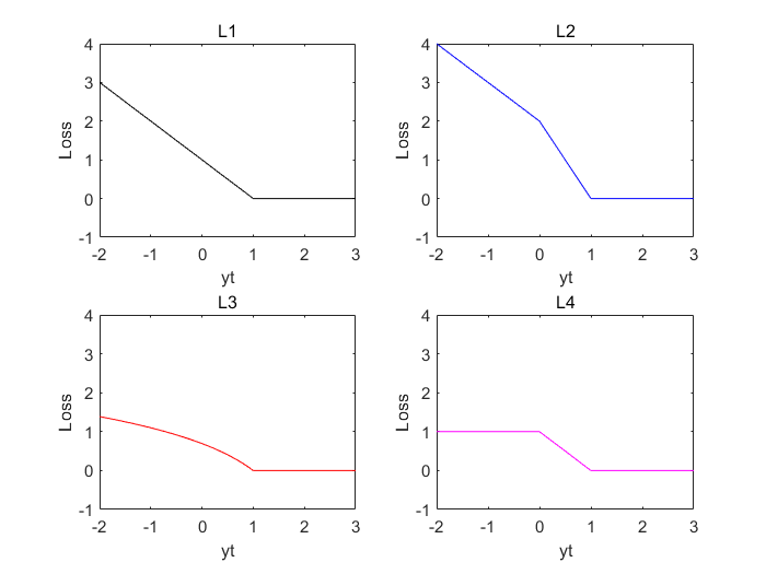
In this section, we test Algorithm 1 by the synthetic data and the real data. We choose some training data and testing data, loss functions and kernels to test Algorithm 1. For simplicity, let L1L_{1}, L2L_{2}, L3L_{3} and L4L_{4} be four loss functions used in our experiments, that is,

L1​(𝒙,y,t)={1−y​t,y​t−1<00,y​t−1≥0,L2​(𝒙,y,t)={−y​t+2,y​t−1<−1−2​y​t+2,−1≤y​t−1<00,y​t−1≥0,L_{1}(\boldsymbol{x},y,t)=\begin{cases}1-yt,&yt-1<0\\ 0,&yt-1\geq 0\end{cases},\ \ L_{2}(\boldsymbol{x},y,t)=\begin{cases}-yt+2,&yt-1<-1\\ -2yt+2,&-1\leq yt-1<0\\ 0,&yt-1\geq 0\end{cases},

and

L3​(𝒙,y,t)={l​o​g​(2−y​t),y​t−1<00,y​t−1≥0,L4​(𝒙,y,t)={1,y​t−1<−11−y​t,−1≤y​t−1<00,y​t−1≥0.L_{3}(\boldsymbol{x},y,t)=\begin{cases}log(2-yt),&yt-1<0\\ 0,&yt-1\geq 0\end{cases},\ \ L_{4}(\boldsymbol{x},y,t)=\begin{cases}1,&yt-1<-1\\ 1-yt,&-1\leq yt-1<0\\ 0,&yt-1\geq 0\end{cases}.

Here are the graphs of these support vector loss functions above.
Refer to caption
Figure 1: For the graphs of the loss functions L1L_{1}, L2L_{2}, L3L_{3} and L4L_{4}, we replace y​tyt to tt because of the symmetry of y=+1y=+1 and y=−1y=-1.

We see that L1L_{1} is convex Hinge loss, L2L_{2} is a nonconvex linear piecewise loss function, L3L_{3} is a nonconvex piecewise logarithmic loss function and L4L_{4} is a nonconvex ramp loss function. These four loss functions satisfy Assumption 4.1. On the other hand, let K1K_{1} be Gaussian kernel, that is,

K1​(𝒙,𝒙′)=exp⁡(−σ1​‖𝒙−𝒙′‖22),for​σ1>0K_{1}(\boldsymbol{x},\boldsymbol{x}^{\prime})=\exp(-\sigma_{1}\|\boldsymbol{x}-\boldsymbol{x}^{\prime}\|_{2}^{2}),\ \text{for}\ \sigma_{1}>0

and K2K_{2} be Matérn 1-norm kernel, that is,

K2​(𝒙,𝒙′)=exp⁡(−σ2​‖𝒙−𝒙′‖1),for​σ2>0,K_{2}(\boldsymbol{x},\boldsymbol{x}^{\prime})=\exp(-\sigma_{2}\|\boldsymbol{x}-\boldsymbol{x}^{\prime}\|_{1}),\ \text{for}\ \sigma_{2}>0,

where ∥⋅∥1\|\cdot\|_{1} denotes 1-norm in Euclidean space. Moreover, these two kernels are symmetric and strictly positive definite. Next we introduce our test results on synthetic data and real data.

5.1 Examples on Synthetic Data

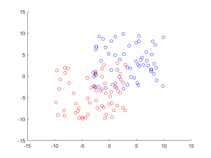
We sample from Ω1=[−3,10]×[−3,10]\Omega_{1}=[-3,10]\times[-3,10] labeled by +1+1 and Ω2=[−10,3]×[−10,3]\Omega_{2}=[-10,3]\times[-10,3] labeled by −1-1 randomly to obtain different training sets and testing sets. The data labeled by +1+1 are equal to the data labeled by −1-1 in each training set or testing set. Here is an example of sampling. In the following figures, two subdatasets are colored in blue and red.

Refer to caption
(a) Training Set
Refer to caption
(b) Testing Set
Figure 2: Example of Sampling (N=300)(N=300).

First, we show the convergence of Algorithm 1 for the nonconvex loss function L3L_{3}. Some parameters and results of the numerical experiment represent as follows.

  • •

    Gaussian kernel K1K_{1}, where σ1=1\sigma_{1}=1.

  • •

    The nonconvex loss function L3L_{3}.

  • •

    N=300N=300.

  • •

    λ=0.1\lambda=0.1, ρ=0.05\rho=0.05 and ε0=10−12\varepsilon_{0}=10^{-12}.

  • •

    we choose initial values randomly in [−10,10]N[-10,10]^{N}.

From (4.22), we can show the convergence of {sk}\{s^{k}\} by ∑k=1∞‖sk+1−sk‖ℋ\sum\limits_{k=1}^{\infty}\|s^{k+1}-s^{k}\|_{\mathcal{H}}. By definition of {sk}\{s^{k}\}, (3.1) and (3.2), we have that

‖sk+1−sk‖ℋ=∑i=1N(𝒄k+1−𝒄k)i​(sk+1−sk)​(𝒙i)=(𝒄k+1−𝒄k)T​A​(𝒄k+1−𝒄k).\|s^{k+1}-s^{k}\|_{\mathcal{H}}=\sqrt{\sum_{i=1}^{N}(\boldsymbol{c}^{k+1}-\boldsymbol{c}^{k})_{i}(s^{k+1}-s^{k})(\boldsymbol{x}_{i})}=\sqrt{(\boldsymbol{c}^{k+1}-\boldsymbol{c}^{k})^{T}A(\boldsymbol{c}^{k+1}-\boldsymbol{c}^{k})}.

In the following two picture, we show the convergence of Algorithm 1 by ∑k=1∞‖sk+1−sk‖ℋ\sum\limits_{k=1}^{\infty}\|s^{k+1}-s^{k}\|_{\mathcal{H}}.

Refer to caption
(a) ‖sk+1−sk‖ℋ\|s^{k+1}-s^{k}\|_{\mathcal{H}}
Refer to caption
(b) ∑k=1∞‖sk+1−sk‖ℋ\sum_{k=1}^{\infty}\|s^{k+1}-s^{k}\|_{\mathcal{H}}
Figure 3: Convergence of Algorithm 1 with Nonconvex Loss Function L3L_{3}.

Figure 3 shows that for the training data and parameters, Algorithm 1 converges in 61 iterations. This shows the effectiveness of Algorithm 1. Next, we use different sizes of training set and testing set to test Algorithm 1. Some parameters and results of the numerical experiment represents as follows.

  • •

    Gaussian kernel K1K_{1}, where σ1=1\sigma_{1}=1.

  • •

    The nonconvex loss function L2L_{2}.

  • •

    N=300N=300.

  • •

    λ=0.1\lambda=0.1, ρ=1\rho=1 and ε0=10−12\varepsilon_{0}=10^{-12}.

  • •

    we choose 20 initial values randomly in [−10,10]N[-10,10]^{N}.

Table 1: Comparison of Different Sizes of Data.
Training Data Testing Data Time(s) Training Accuracy Testing Accuracy
100 40 3.546 98% 85%
200 80 7.302 94% 87.5%
300 120 10.524 93.7% 90%
400 160 14.833 93% 87.5%
500 200 18.343 93.2% 90%
600 240 21.813 92.7% 87.1%
700 280 27.469 92.4% 89.3%
800 320 33.776 92.1% 90.9%
900 360 44.653 90.3% 90%
1000 400 56.510 92.3% 89%

Table 5.2 shows that solving Optimization (2.1) by Algorithm 1 is feasible in terms of running time and accuracy. Next we will show that choosing different kinds of loss functions and kernels have different accuracy.

Now we sample from the area Ω1\Omega_{1} and Ω2\Omega_{2} randomly to obtain a training set with 300300 points and a testing set with 120120 points. Some parameters of these experiments represent as follows.

  • •

    The kernels K1K_{1} and K2K_{2}, where σ1=2\sigma_{1}=2 and σ2=1\sigma_{2}=1.

  • •

    The loss functions L1L_{1}, L2L_{2}, L3L_{3} and L4L_{4}.

  • •

    λ=0.5\lambda=0.5, ρ=5\rho=5 and ε0=10−12\varepsilon_{0}=10^{-12}.

  • •

    Choose 2020 initial values randomly in [−10,10]N[-10,10]^{N}.

In each experiment, we will choose a loss function and a kernel. The results of these experiments represent as follows.

Table 2: Numerical Results of Using Different Loss Functions and Kernels.
Loss Function Kernel Training Accuracy Testing Accuracy
L1L_{1} K1K_{1} 95.7% 87.5%87.5\%
L2L_{2} K1K_{1} 95% 88.3%88.3\%
L3L_{3} K1K_{1} 95.7% 88.3%88.3\%
L4L_{4} K1K_{1} 95% 87.5%87.5\%
L1L_{1} K2K_{2} 92% 90.8%90.8\%
L2L_{2} K2K_{2} 93.7% 90%90\%
L3L_{3} K2K_{2} 94.7% 90.8%90.8\%
L4L_{4} K2K_{2} 93% 90%90\%

From Table 2, it is easy to see that the nonconvex loss function L3L_{3} performs better than L1L_{1}, L2L_{2} and L4L_{4} in these experiments. It shows that the SVM in the RKHS with the nonconvex loss function is better than the SVM in the RKHS with the convex loss functions for some cases. Next, we introduce the numerical experiment results on a real-world benchmark dataset.

5.2 Examples on UCI Machine Learning Repository

The vinho verde data in UCI machine learning repository has two kinds of wine samples. We will identify them based on physicochemical tests. There are 11 input variables about them, which are fixed acidity, volatile acidity, citric acid, residual sugar, chlorides, free sulfur dioxide, total sulfur dioxide, density, pH, sulphates and alcohol. We have 2000 wine samples in training set, and a half of them are labeled by +1 and the others are labeled by -1. Moreover, we have 718 wine samples in testing set, and a half of them are labeled by +1 and the others are labeled by -1. Next, we introduce some parameters of these experiments as follows.

  • •

    The kernels K1K_{1} and K2K_{2}, where σ1=5\sigma_{1}=5 and σ2=5\sigma_{2}=5.

  • •

    The loss functions L1L_{1}, L2L_{2}, L3L_{3} and L4L_{4}.

  • •

    λ=0.5\lambda=0.5, ρ=1\rho=1 and ε0=10−12\varepsilon_{0}=10^{-12}.

  • •

    Choose 2020 initial values randomly in [−10,10]N[-10,10]^{N}.

In each experiment, we will choose a loss function and a kernel and we have the following results.

Table 3: Numerical Results on Vinho Verde Data.
Loss Function Kernel Training Accuracy Testing Accuracy
L1L_{1} K1K_{1} 99,9% 90.0%90.0\%
L2L_{2} K1K_{1} 100% 90.8%90.8\%
L3L_{3} K1K_{1} 99.9% 90.3%90.3\%
L4L_{4} K1K_{1} 99.9% 90.3%90.3\%
L1L_{1} K2K_{2} 100% 88.3%88.3\%
L2L_{2} K2K_{2} 100% 91.8%91.8\%
L3L_{3} K2K_{2} 100% 87.6%87.6\%
L4L_{4} K2K_{2} 100% 91.2%91.2\%

From Table 3, we check that L2L_{2} performs better than L1L_{1}, L3L_{3} and L4L_{4}. It shows that in some cases the nonconvex loss function is more suitable than the convex loss function, which is our motivation of this paper.

In Section 5, we demonstrate the effectiveness of solving Optimization (2.1) by Algorithm 1. In addition, we give some examples to show that in some cases, the SVM in the RKHS with the nonconvex loss functions are better than the SVM in the RKHS with the convex loss functions. Therefore, we should reconsider not only convex loss function but also nonconvex loss function.

Acknowledgments. This program is supported by the National Natural Science Foundation of China under grant #12071157, #12026602 and the Natural Science Foundation of Guangdong #2019A1515011995 and #2020B1515310013.

References

  • [1] A. Beck. First-Order Methods in Optimization. SIAM, Philadelphia, 2017.
  • [2] J. Bolte, A. Daniilidis and A. Lewis. The Lojasiewicz inequality for nonsmooth subanalytic functions with applications to subgradient dynamical systems. SIAM J. Optimiz. 17 (2007), 1205-1223.
  • [3] J. Bolte, A. Daniilidis, A. Lewis and M. Shiota. Clarke subgradients of stratifiable functions. SIAM J. Optimiz. 18 (2007), 556-572.
  • [4] J. Bolte, S. Sabach and M. Teboulle. Proximal alternating linearized minimization for nonconvex and nonsmooth problems. Math. Program. 146 (2014), 459-494.
  • [5] S. Boyd, N. Parikh, E. Chu, B. Peleato, J. Eckstein, et al. Distributed optimization and statistical learning via the alternating direction method of multipliers. Found. Trends. Mach. Le. 3 (2011), 1-122.
  • [6] J. Brooks. Support Vector Machines with Ramp Loss and the Hard Margin Loss. Oper. Res. 59 (2011), 467-479.
  • [7] C. Cortes and V. Vapnik. Support Vector Network. Mach. Learn. 20 (1995), 273-297.
  • [8] H. Dales, F. Dashiell, A. Tau and D. Strauss. Banach Spaces of Continuous Functions as Dual Spaces. Springer, Switzerland, 2016.
  • [9] Y. Feng, Y. Yang, S. Huang, S. Mehrkanoon and J. Suykens. Robust Support Vector Machines for Classification with Nonconvex and Smooth Losses. Neural Comput. 28 (2016), 1217-1247.
  • [10] F. Facchinei and J. Pang. Finite-Dimensional Variational Inequalities and Complementarity Problems, vol.I. Springer, Berlin, 2003.
  • [11] K. Guo, D. Han and T. Wu. Convergence of alternating direction method for minimizing sum of two nonconvex functions with linear constraints. Int. J. Comput. Math. 94 (2016), 1-18.
  • [12] L. Huang, C. Liu, L. Tan and Q. Ye. Generalized representer theorems in Banach spaces. Anal. Appl. 19 (2021), 125-146.
  • [13] D. Kincaid and W. Cheney. Numerical Analysis: Mathematics of Scientific Computing, 3rd Edition. American Mathematical Society, Providence, 2002.
  • [14] G. Li and T. Pong. Global convergence of splitting methods for nonconvex composite optimization. SIAM J. Optimiz. 25 (2015), 2434-2460.
  • [15] D. Liu, Y. Shi, Y. Tian and X. Huang. Ramp loss least squares support vecotr machine. J. Comput. Sci-Neth. 14 (2016), 61-68.
  • [16] R. Megginson. An Introduction to Banach Space Theory. Springer-Verlag, New York, 1998.
  • [17] B. Mordukhovich. Variational Analysis and Generalized Differentiation. I: Basic Theory. Grundlehren Series (Fundamental Principles of Mathematical Sciences), Springer, Berlin, 2006.
  • [18] S. Park and Y. Liu. Robust Penalized Logistic Regression with Truncated Loss Functions. Can. J. Stat. 39 (2011), 300-323.
  • [19] F. Pérez-Cruz, A. Navia-Vázquez, A. Figueiras-Vidal and A. Artés-Rodríguez. Empirical risk minimization for support vector classifiers. IEEE Trans. Neural Netw. 14 (2003), 296-303.
  • [20] R. Rockafellar and R. Wets. Variational Analysis. Springer Berlin Heidelberg, Berlin, 1998.
  • [21] W. Rudin. Principles of mathematical analysis. McGraw-Hill, Inc, New York, 1976.
  • [22] X. Shen, L. Niu, Z. Qi. and Y. Tian, Support Vector Machine Classifier with Truncated Pinball Loss. Pattern Recogn., 68 (2017), 199-210.
  • [23] M. Shiota. Geometry of Subanalytic and Semialgebraic Sets. Birkhäuser, Boston, 1998.
  • [24] I. Steinwart and A. Christmann. Support Vector Machines. Springer-Verlag, New York, 2008.
  • [25] H. Wang, Y. Shao, S. Zhou, C. Zhang and N. Xiu. Support vector machine classifier via L0/1 soft-margin loss. IEEE T. Pattern Anal. 2021, doi:10.1109/TPAMI.2021.3092177, in press.
  • [26] H. Wendland. Scattered Data Approximation. Cambridge University Press, Cambridge, 2005.
  • [27] Y. Xu and Q. Ye. Generalized Mercer kernels and reproducing kernel Banach spaces. Mem. Am. Math. Soc. 258 (2019), 1-122.
  • [28] Y. Xu and W. Yin. A block coordinate descent method for regularized multiconvex optimization with applications to nonnegative tensor factorization and completion. SIAM J. Imaging Sci. 6 (2013), 1758–1789.
  • [29] L. Yang and H. Dong. Support Vector Machine with Truncated Pinball Loss and its Application in Pattern Recognition. Chemometr. Intell. Lab. 177 (2018), 89-99.
  • [30] C. Zalinescu. Convex Analysis in General Vector Spaces. World Scientific Publishing, River Edge, 2002.


MINGYU MO

School of Mathematical Sciences

South China Normal University

Guangzhou, 510631, Guangdong, PR China

Email-address: mmymaths@qq.com.

QI YE

School of Mathematical Sciences

South China Normal University

Guangzhou, 510631, Guangdong, PR China

Pazhou Lab

Guangzhou, 511442, Guangdong, PR China.

Email-address: yeqi@m.scnu.edu.cn.