A Feedforward Unitary Equivariant Neural NetworkJournal: ???

In general, given a function $\phi:\mathcal{X}\rightarrow\mathcal{Y}$ (where the domain $\mathcal{X}$ and the co-domain $\mathcal{Y}$ might be different) and a group $G$, we assume that each element $g\in G$ induces group actions $T_{g}:\mathcal{X}\rightarrow\mathcal{X}$ and $\widehat{T}_{g}:\mathcal{Y}\rightarrow\mathcal{Y}$ on $\mathcal{X}$ and $\mathcal{Y}$, respectively. Then, the function $\phi$ is equivariant under $G$ if for all $g\in G$ and $x\in\mathcal{X}$, the following holds:

Formally, a group action needs to satisfy $T_{g_{1}g_{2}}=T_{g_{1}}\circ T_{g_{2}}$ for all $g_{1},g_{2}\in G$.

Invariant is the special case when for all $g\in G$, the group action $\widehat{T}_{g}$ is the identity function on $\mathcal{Y}$.

In this paper, we consider domains of the form $\mathbb{C}^{n\times M}$, which we interpret as $M$ points in $\mathbb{C}^{n}$. We consider the unitary group $U(n)$, where each element corresponds to a unitary operator $\mathcal{U}$ on $\mathbb{C}^{n}$. The unitary group contains the orthogonal group $O(n)$ (that corresponds to rotations and reflections) and $SO(n)$ (that corresponds to rotations only).

Given a unitary operator $\mathcal{U}:\mathbb{C}^{n}\rightarrow\mathbb{C}^{n}$, the group action on $M$ points are defined by

We construct a feedforward neural network with $L-1$ hidden layers. The input layer is labelled as the $0^{th}$ layer, and the output layer is the $L^{th}$ layer. For the $(k+1)^{th}$ layer, its input is from the $k^{th}$ layer:

where $M_{k}$ is the number of vector elements of

Each vector element $\mathbf{x}_{k}^{(\alpha)}\in\mathbb{C}^{n}$ is an $n$-dimensional vector. Similarly, we have the output

We define a variable

This definition is different from conventional feedforward NN. First, the $\mathbf{x}_{k}$ is a matrix and is put on the left-hand side of the weight parameter. Second, a new matrix variable $\mathbf{e}_{k}$ is introduced. These two changes are crucial steps to avoid the need to perform convolution. It allows the unitary operator getting out naturally from the left-hand side of $\mathbf{x}_{k}$ and $\mathbf{e}_{k}$.

The weight and bias parameters matrices

and

where $||.||$ is the norm of an $n$-dimensional vector. Observe that for any unitary operator $\mathcal{U}$, it holds that

For all $\alpha\in\{1,2,...,M_{k}\}$, we can obtain

where $\mathcal{U}$ is applied element-wise on each $\mathbf{x}_{k}^{(\alpha)}$.

Then, we define an activation function

for the $(k+1)^{th}$ layer. The activation function acts on each vector $\mathbf{y}_{k}^{(\alpha)}\in\mathbb{C}^{n}$ in element-wise manner. We note $\mathbf{y}_{k}$ has the same dimension of $\mathbf{x}_{k+1}$.

We shall find an activation function that satisfies the following:

This completes the construction of our feedforward equivariant neural network for unitary transformations.

Observe that each layer is equivariant with respect to unitary operators in the sense of equation (1). The reason is that if we transform the input $\mathbf{x}_{k}\rightarrow\mathcal{U}\mathbf{x}_{k}$, then its output will undergo the transformation $\mathbf{x}_{k+1}\rightarrow\mathcal{U}\mathbf{x}_{k+1}$; in this case, the unitary operator can act element-wise on both the input and the output spaces. Therefore, when we apply the group action, which is now the unitary operator $\mathcal{U}$, on the $0^{th}$ layer input $\mathbf{x}_{0}$, the same operator will propagate to the final layer output $\mathbf{x}_{L}$. It means if we put $\mathbf{x}_{0}\rightarrow\mathcal{U}\mathbf{x}_{0}$, the output will become $\mathbf{x}_{L}\rightarrow\mathcal{U}\mathbf{x}_{L}$.

A possible choice of the activation function for each element can be a softsign function with a small residue, that is

where $a$ is a (small) scalar constant, and $\mathbf{u}\in\mathbb{C}^{n}$. The small residue is to avoid vanishing gradient of Loss function when $\mathbf{u}$ is large. We used this activation function in our numerical experiment.

Alternatively, one may choose the identity function, that is

which in scalar form is a popular choice of activation function for the output layer. Similarly, ReLu function and Leaky ReLu function in vector forms are also equivariant with respect to unitary operators.

We can introduce extra scalar features into our ENN, in addition to vector elements. The idea is that we will increase the number of coordinates from $n$ to $n+m$, and we only consider unitary operations that do not change the extra $m$ coordinates.

Formally, for each input $\mathbf{x}_{0}^{(\alpha)}$, we assume that it has $m$ corresponding scalar features which can be written as a vector $\mathbf{h}_{0}^{(\alpha)}=\{h_{0,1}^{(\alpha)},h_{0,2}^{(\alpha)},...,h_{0,m}^{(\alpha)}\}$, we can rewrite the input vector element into

and the unit vector

where $\mathbf{1}$ is a vector with $m$ elements and all equal $1$. (Observe that in the actual implementation, we can reduce $\mathbf{1}$ and the associated weights in the model to a single scalar bias term.)

The operator can be rewritten in matrix form such that

where $\mathbf{I}$ is an identity $m\times m$ matrix. Plugging them back to equations in previous subsection, they all hold, provided that the definition of norm can fulfill, i.e.

It essentially means we only apply the group action on part of the input vectors, and keep the features part of the vectors fixed. Features can be anything that are quantifiable, such as color, brightness, contrast, electronic charge, mass, humidity, level of pollutant, and etc.

Although at the output layer, we will get outputs ${\mathbf{x}^{\prime}}_{L}\in\mathbb{C}^{(n+m)\times M_{L}}$, the Loss function can be defined only using part of it. We also need to be careful that ${\mathbf{x}^{\prime}}_{L}$ does not need to have the same unit or meaning as ${\mathbf{x}^{\prime}}_{0}$. For example, if we considers a system of molecules, we may use positions as the vector elements, and charges and masses as features. It means we have vector inputs in $\mathbb{R}^{(3+2)\times M_{0}}$. Even we have vector outputs $\mathbb{R}^{(3+2)\times M_{L}}$, the prediction can be forces, atomic energy, and a dummy value that does not enter the Loss function. On the other hand, one can also add dummy input features to make each element in ${\mathbf{x}^{\prime}}_{0}$ and ${\mathbf{x}^{\prime}}_{L}$ longer.

We can derive an algorithm similar to the commonly known backpropagation. The essence of backpropagation is to reuse the information of the gradient of the Loss function with respect to the elements in weight and bias parameters. First, we define our Loss function:

where $\mathbf{T}\in\mathbb{C}^{n\times M_{L}}$ is the target data, and $C$ is a non-negative real value function being differentiable with respect to $\bm{\sigma}_{L}$. For convenient, we write a combined representation of the weight and bias parameters, such that $\mathbf{z}_{k}=\{\mathbf{W}_{k},\mathbf{b}_{k}\}$. For each element in $\mathbf{z}_{L-1}$, the derivative

where

For other layers, in general, we can write

where

This allows us to reuse the information of $\bm{\delta}_{L-k}$ in $\bm{\delta}_{L-k-1}$. However, it is different from the conventional backpropogation, where the whole derivative of the deeper layer is reused. We only use a part of the derivative in our backpropagation procedure.

The above construction of ENN has no permutation symmetry yet. We say that a function $\phi$ having $n$ inputs achieves permutation symmetry, if for any permutation $\pi$ on $\{1,2,\ldots,n\}$ and any $(x_{1},\ldots,x_{n})$,

The order and the number of inputs of $\phi$ are fixed. In some applications, we may partition the inputs and consider permutations within each part. For instance, we can partition the inputs into $\mathcal{S}_{a}=\{1,2,\ldots,m\}$ and $\mathcal{S}_{b}=\{m+1,\ldots,n\}$ such that for any permutations $\pi_{a}$ and $\pi_{b}$ on the corresponding parts, permutation symmetry means:

Permutation symmetry should hold in some physical systems. For example, if we have a molecular composed of H, C and O atoms, then each input corresponds to an atom and the inputs can be partitioned according to the type of atom. Then, atoms in each part can be permuted without affecting the output.

One way to achieve permutation symmetry is to introduce a pre-processing step in the first layer. Suppose there are $N_{0}$ input vectors denoted by $(\mathbf{u}^{(\xi)}\in\mathbb{C}^{n}:\xi\in\{1,2,...,N_{0}\})$. This step produces $M_{0}$ vectors via a collection of functions $\mathbf{D}^{(\alpha)}:\mathbb{C}^{n\times N_{0}}\rightarrow\mathbb{C}^{n}$ for each $\alpha\in\{1,2,...,M_{0}\}$. Since our final neural network achieves equivariance, we require that for any unitary operator $\mathcal{U}$, the following holds:

In addition to being equivariant for unitary operators, we describe how each $\mathbf{D}^{(\alpha)}$ also achieves permutation symmetry.

We can also express the idea of partitioning the $n$ inputs and consider permutation symmetry within each part. For example, each part is indexed by $\delta$ (also known as a feature), and an index $i$ having feature $\delta$ can be represented by $v_{i\delta}=1$ and 0, otherwise. Then, we can consider the following function:

where the trainable weights $w_{\delta}$ again does not depend on the index $i$. Observe that if indices $i$ having the same feature $\delta$ are permuted, the value of the function does not change.

If we now consider a system of atoms, for atom $i$, it has $N_{0}$ neighbors within a cutoff distance $r_{c}$. $\{\mathbf{r}_{j}\in\mathbb{R}^{3}|r_{ij}<r_{c}\}$ is the set of positions of neighboring atoms of atom $i$. We may consider each atom as a node. As a special case, one can put

where the interatomic distance between atom $i$ and $j$ is $r_{ij}=|\mathbf{r}_{ij}|=|\mathbf{r}_{j}-\mathbf{r}_{i}|$. The $f_{c}$ is a scalar smooth-out function such that at the cut-off distance $r_{c}$, $f_{c}(r_{c})=0$, and is continuous and differentiable up to at least second derivatives. This is similar to the implementation in SchNet (Schütt et al. 2018).

We further assume there is only one feature corresponding to $\delta$, where $v_{j1}=1$, the weight is a Kronecker delta function $w_{\beta 1\alpha}=\delta_{\beta\alpha}$, and the activation function is an identity function. Equation 29 becomes:

where $\alpha\in\{1,2,...,M_{0}\}$. The set of hyper-parameters $\{\eta^{(\alpha)},r_{s}^{(\alpha)}\}$ are predetermined values. Interestingly, this is in the same functional form as suggested by Behler and Parrinello 2007 who mapped the local atomic environment to a set of atom-centered symmetry functions (or called spatial descriptors) and used them to develop machine-learned (ML) interatomic potential.

Following similar logic, one may devise a set of vector function by augmenting above scalar spatial descriptor, such that

It is straightforward to check

which resembles equation 26. The subscribe $j$ here is corresponding to the superscribe $(\xi)$ of $\mathbf{u}$ in equation 26.

We are not going to show any example on this. It is only to show theoretically that one can introduce permutation symmetry by adding an extra layer of properly designed vector form GNN to our ENN.

Our implementation has the limitation that the group action on the input data is the same group action on the output data, and the group action is restricted to unitary transformation. Therefore, if one applies the unitary operator on the input data, but the target data does not experience the same transformation, our method does not apply.

For example, in physical systems, quantities can have odd or even parity symmetry, e.g., consider the parity transformation $\mathcal{P}:(x,y,z)\mapsto(-x,-y,-z)$. For quantities with odd parity symmetry, they will have sign change according to the parity transformation. Our ENN can be applied to predict these quantities. However, for vector quantities with even parity symmetry, our ENN does not apply. For example, in classical mechanics, the angular momentum

If we apply the parity transformation, we get $\mathbf{r}\rightarrow\mathbf{-r}$ and $\mathbf{p}\rightarrow\mathbf{-p}$, but we still get

If we use $\mathbf{r}$ and $\mathbf{p}$ as the input data, we cannot use our ENN to predict $\mathbf{L}$. A possible solution is to manually apply sign change to the output data according to the input data.

For scalar quantities with even parity symmetry, it can be remedied by converting $\mathbf{x}_{k}$ at arbitrary $k$ layers, where $\mathbf{x}_{k}\in\mathbb{C}^{n\times M_{k}}$, to invariant scalar quantities. For examplem we can set $\mathbf{w}_{p}$ as a function of $\mathbf{x}_{k}$, where $\mathbf{w}_{p}\in\mathbb{C}^{M_{p}}$, and plug $\mathbf{w}_{p}$ into other implementations of neural networks with $M_{p}$ scalar inputs. An obvious example is the scalar spatial descriptors for predicting the interatomic potential energy (Behler and Parrinello 2007) as mentioned in previous subsection, where energy has even parity symmetry.

We simulate a system of 4-body motion governed by a Hamiltonian model. Our aim is to predict the forces when atoms are locating at different positions, and simulate the dynamics. We generate data using a well defined physical model, which allows us to examine the errors.

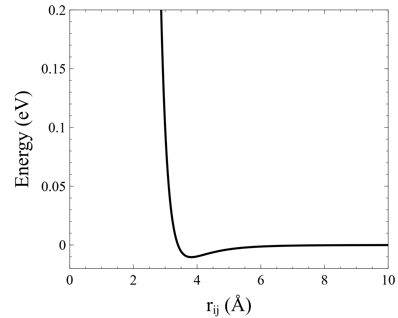
We adopt a pair-wise Lennard-Jones potential for Argon (Rahman 1964):

where $\epsilon/k_{B}=120$ Kelvin, $r_{0}=3.4$Å, and $k_{B}$ is the Boltzmann constant. A plot of the potential energy is shown in Figure 1.

The interatomic potential energy of the system is written as a sum of pair-wise interaction energies:

where $r_{ij}=|\mathbf{r}_{i}-\mathbf{r}_{j}|$. The force acting on atom $i$ is

We generate 100,000 set of positions in three dimensional space. Each set contains the positions of 4 atoms. The $x$, $y$, and $z$ coordinates of each atom is generated randomly according to the Gaussian distribution with mean equals zero and standard deviation equals 3Å. Then, we calculate the interatomic distance of each pair of atoms. If any of them smaller than $r_{min}=2.8$Å, we discard this set of positions and generate a new one. We repeat this procedure until no interatomic distance is small than $r_{min}$. This is to avoid the occurrence of very large atomic force due to small separation. We can readily understand it by inspecting Fig. 1. The energy have a drastic increase at around 3Å. Atoms can hardly be in such small separation in dynamic simulations. Using these positions, we can obtain a set of four atomic forces for each set of positions using the Lennard-Jones potential.

Instead of using the positions as inputs directly, we use the relative positions as inputs:

This takes care of the translational symmetry.

The target data are simply the atomic forces:

We rescale both the input and output data by their standard deviations before we use them to train an ENN. Data are split, where 60% is for training, 20% is for validation, and 20% for testing.

The relationship between the input and output data is learned by an ENN, which has five hidden layers. The number of nodes in each layers counting from input to output layers are 6, 50, 90, 100, 80, 50, and 4.

The loss function is the mean-squared error, which is defined as

where $N_{data}$ is the number of used data and $\mathbf{x}_{L}$ is the output data. The weight parameters $\mathbf{W}$ are initialized according to normalized Xavier method (Glorot and Bengio 2010). The bias parameters $\mathbf{b}$ are initialized to zeros.

The training of ENN is performed through minimizing the loss function with respect to $\{\mathbf{W},\mathbf{b}\}$. We used the FIRE algorithm (Bitzek et al. 2006). It is a minimization method commonly used for relaxing atomic structures. It is similar to the Nesterov momentum method (Nesterov 1983), and has fast convergence behavior in practice. We briefly discuss the method and our adaptation in Appendix.

Fig. 2 shows the change of the value of the loss function calculated using the training data and the validation data. We performed 10 million iterations. We see that both of them drop significantly. As expected, the training loss drops faster than validation loss. However, it seems that the model does not suffer from overfitting. We stop the iteration process as soon as we observe fluctuations in the training loss, i.e., further iterations might actually increase the training loss.

Using testing data, we can calculate the atomic forces analytically according to the Lennard-Jones potential and predict them by our trained ENN. In Fig. 3, the analytical and predicted values are plotted against each others. We plotted all the $x$, $y$, and $z$ components of the data. The root mean square deviation (RMSD) is 0.00118 eV/Å. Observe that the training data are in the order of 0.1 to 1 eV/Å, and the average error is in the order of 0.001 eV/Å, which is fairly satisfactory.

We use the forces predicted by our trained ENN to drive the evolution of a system of four Argon atoms using molecular dynamics (MD). We will also compare our predictions with analytical solutions. Note that our ENN was not trained to any trajectory of atomic motion. All training data are static. No history dependent information was involved in the training.

The motion of atoms are governed by the Newton’s equations

where the position and momentum of atom $i$ are $\mathbf{r}_{i}\in\mathbb{R}^{3}$, $\mathbf{p}_{i}\in\mathbb{R}^{3}$ and the atomic mass is $m_{i}$.

Using our trained ENN, we can predict the atomic forces $\{\mathbf{F}_{i}\}$. On the other hand, if the analytical form of a Hamiltonian is known, the atomic force is

where the Hamiltonian is:

Without introducing perturbation and dissipation, this dynamic system is a closed system, and so the total energy should conserve.

We initialized ten samples. The positions of Argon atoms are initialized at $(3,0,0.1)$, $(-3,-0.1,0)$, $(0.1,2.5,0)$, and $(0,-2.5,-0.1)$, where unit is in Å. Velocities are generated randomly with kinetic energy corresponding to a temperature of 10 Kelvin. The mass of an Argon atom is 39.948$u$. We integrated Newton’s equation using velocity Verlet algorithm. We used a time step of 1fs, which is a conventional value for MD simulations.

We calculated the RMSD of the positions of atoms. It is defined as:

where $N_{s}=10$ is the number of sample, $N_{at}=4$ is the number atoms in a sample, $\mathbf{r}_{i}^{a}$ is the position of atom $i$ calculated according to analytical solution, and $\mathbf{r}_{i}^{p}$ is the position calculated using forces predicted by ENN.

Fig. 4 shows the RMSD of positions as a function of MD steps. As expected, they deviate more and more as a function of steps, because the error is accumulating throughout the simulation. We may inspect the real trajectory of an atom in Fig. 5. It shows the $x$ component of atom 1 in sample 1. We see the initial 1500 MD steps predictions are fairly good, and up to 4000 MD steps are acceptable. Our ENN shows certain predictive power, and the predictions are three dimensional vectors.

We calculated the RMSD of the system energies. It is defined as:

where $E^{a}$ and $E^{p}$ are the total energy calculated using equation 46. The potential energy are calculated using the positions of atoms that evolve according to forces calculated analytically or by prediction using ENN.

Fig. 6 shows the RMSD of energy across ten samples. Again, we can see the deviation accumulates. However, we should remember that in the training of ENN, we did not provide any information about energy to the training. If we look at around 4000 steps, the RMSD is less than about $4\times 10^{-4}$ eV, which is about 2 order of magnitude smaller than the system energy. Our results are encouraging. It shows that even if we don’t know the system total energy (or Hamiltonian), we can still predict forces, which are vectors, using our ENN. We can also predict multiple forces at the same time.

References

- Bartók et al. (2010) Bartók, A.P., Payne, M.C., Kondor, R., Csányi, G., 2010. Gaussian approximation potentials: The accuracy of quantum mechanics, without the electrons. Phys. Rev. Lett. 104, 136403. URL: https://link.aps.org/doi/10.1103/PhysRevLett.104.136403, doi:10.1103/PhysRevLett.104.136403.
- Batzner et al. (2022) Batzner, S., Musaelian, A., Sun, L., Geiger, M., Mailoa, J.P., Kornbluth, M., Molinari, N., Smidt, T.E., Kozinsky, B., 2022. E(3)-equivariant graph neural networks for data-efficient and accurate interatomic potentials. Nature communications 13, 1–11.
- Behler and Parrinello (2007) Behler, J., Parrinello, M., 2007. Generalized neural-network representation of high-dimensional potential-energy surfaces. Physical Review Letters 98, 146401.
- Bitzek et al. (2006) Bitzek, E., Koskinen, P., Gähler, F., Moseler, M., Gumbsch, P., 2006. Structural relaxation made simple. Phys. Rev. Lett. 97, 170201. URL: https://link.aps.org/doi/10.1103/PhysRevLett.97.170201, doi:10.1103/PhysRevLett.97.170201.
- Brandstetter et al. (2022) Brandstetter, J., Welling, M., Worrall, D.E., 2022. Lie point symmetry data augmentation for neural PDE solvers, in: ICML.
- Cobb et al. (2021) Cobb, O., Wallis, C.G.R., Mavor-Parker, A.N., Marignier, A., Price, M.A., d’Avezac, M., McEwen, J., 2021. Efficient generalized spherical CNNs, in: International Conference on Learning Representations. URL: https://openreview.net/forum?id=rWZz3sJfCkm.
- Cohen and Welling (2016) Cohen, T., Welling, M., 2016. Group equivariant convolutional networks, in: Balcan, M.F., Weinberger, K.Q. (Eds.), Proceedings of The 33rd International Conference on Machine Learning, PMLR, New York, New York, USA. pp. 2990–2999. URL: https://proceedings.mlr.press/v48/cohenc16.html.
- Cohen et al. (2018) Cohen, T.S., Geiger, M., Köhler, J., Welling, M., 2018. Spherical CNNs, in: International Conference on Learning Representations. URL: https://openreview.net/forum?id=Hkbd5xZRb.
- Esteves et al. (2020) Esteves, C., Allen-Blanchette, C., Makadia, A., Daniilidis, K., 2020. Learning SO(3) equivariant representations with spherical CNNs. International Journal of Computer Vision 128, 588–600. URL: https://doi.org/10.1007/s11263-019-01220-1, doi:10.1007/s11263-019-01220-1.
- Gerken et al. (2021) Gerken, J.E., Aronsson, J., Carlsson, O., Linander, H., Ohlsson, F., Petersson, C., Persson, D., 2021. Geometric deep learning and equivariant neural networks. URL: https://arxiv.org/abs/2105.13926, doi:10.48550/ARXIV.2105.13926.
- Glorot and Bengio (2010) Glorot, X., Bengio, Y., 2010. Understanding the difficulty of training deep feedforward neural networks, in: Teh, Y.W., Titterington, M. (Eds.), Proceedings of the Thirteenth International Conference on Artificial Intelligence and Statistics, PMLR, Chia Laguna Resort, Sardinia, Italy. pp. 249–256. URL: https://proceedings.mlr.press/v9/glorot10a.html.
- Hohenberg and Kohn (1964) Hohenberg, P., Kohn, W., 1964. Inhomogeneous electron gas. Phys. Rev. 136, B864–B871. URL: https://link.aps.org/doi/10.1103/PhysRev.136.B864, doi:10.1103/PhysRev.136.B864.
- Kohn and Sham (1965) Kohn, W., Sham, L.J., 1965. Self-consistent equations including exchange and correlation effects. Phys. Rev. 140, A1133–A1138. URL: https://link.aps.org/doi/10.1103/PhysRev.140.A1133, doi:10.1103/PhysRev.140.A1133.
- Kondor (2018) Kondor, R., 2018. N-body networks: a covariant hierarchical neural network architecture for learning atomic potentials. URL: https://arxiv.org/abs/1803.01588, doi:10.48550/ARXIV.1803.01588.
- Kondor et al. (2018) Kondor, R., Lin, Z., Trivedi, S., 2018. Clebsch–Gordan nets: a fully fourier space spherical convolutional neural network, in: Bengio, S., Wallach, H., Larochelle, H., Grauman, K., Cesa-Bianchi, N., Garnett, R. (Eds.), Advances in Neural Information Processing Systems, Curran Associates, Inc. URL: https://proceedings.neurips.cc/paper/2018/file/a3fc981af450752046be179185ebc8b5-Paper.pdf.
- Kondor and Trivedi (2018) Kondor, R., Trivedi, S., 2018. On the generalization of equivariance and convolution in neural networks to the action of compact groups, in: Dy, J., Krause, A. (Eds.), Proceedings of the 35th International Conference on Machine Learning, PMLR. pp. 2747–2755. URL: https://proceedings.mlr.press/v80/kondor18a.html.
- Müller et al. (2021) Müller, P., Golkov, V., Tomassini, V., Cremers, D., 2021. Rotation-equivariant deep learning for diffusion MRI. URL: https://arxiv.org/abs/2102.06942, doi:10.48550/ARXIV.2102.06942.
- Nesterov (1983) Nesterov, Y., 1983. A method for solving the convex programming problem with convergence rate O(). Proceedings of the USSR Academy of Sciences 269, 543–547.
- Rahman (1964) Rahman, A., 1964. Correlations in the motion of atoms in liquid argon. Phys. Rev. 136, A405–A411. URL: https://link.aps.org/doi/10.1103/PhysRev.136.A405, doi:10.1103/PhysRev.136.A405.
- Satorras et al. (2021) Satorras, V.G., Hoogeboom, E., Welling, M., 2021. E(n) equivariant graph neural networks, in: ICML, PMLR. pp. 9323–9332.
- Schütt et al. (2018) Schütt, K.T., Sauceda, H.E., Kindermans, P.J., Tkatchenko, A., Müller, K.R., 2018. SchNet – a deep learning architecture for molecules and materials. The Journal of Chemical Physics 148, 241722. URL: https://doi.org/10.1063/1.5019779, doi:10.1063/1.5019779, arXiv:https://doi.org/10.1063/1.5019779.
- Shapeev (2016) Shapeev, A.V., 2016. Moment tensor potentials: A class of systematically improvable interatomic potentials. Multiscale Modeling & Simulation 14, 1153–1173. URL: https://doi.org/10.1137/15M1054183, doi:10.1137/15M1054183, arXiv:https://doi.org/10.1137/15M1054183.
- Sonoda and Murata (2017) Sonoda, S., Murata, N., 2017. Neural network with unbounded activation functions is universal approximator. Applied and Computational Harmonic Analysis 43, 233–268. URL: https://www.sciencedirect.com/science/article/pii/S1063520315001748, doi:https://doi.org/10.1016/j.acha.2015.12.005.
- Thomas et al. (2018) Thomas, N., Smidt, T., Kearnes, S., Yang, L., Li, L., Kohlhoff, K., Riley, P., 2018. Tensor field networks: Rotation- and translation-equivariant neural networks for 3D point clouds. URL: https://arxiv.org/abs/1802.08219, doi:10.48550/ARXIV.1802.08219.
- Weiler et al. (2018) Weiler, M., Geiger, M., Welling, M., Boomsma, W., Cohen, T.S., 2018. 3D steerable CNNs: Learning rotationally equivariant features in volumetric data, in: Bengio, S., Wallach, H., Larochelle, H., Grauman, K., Cesa-Bianchi, N., Garnett, R. (Eds.), Advances in Neural Information Processing Systems, Curran Associates, Inc. URL: https://proceedings.neurips.cc/paper/2018/file/488e4104520c6aab692863cc1dba45af-Paper.pdf.
- Winkels and Cohen (2018) Winkels, M., Cohen, T.S., 2018. 3D G-CNNs for pulmonary nodule detection, in: Medical Imaging with Deep Learning. URL: https://openreview.net/forum?id=H1sdHFiif.
- Worrall and Brostow (2018) Worrall, D., Brostow, G., 2018. CubeNet: Equivariance to 3D rotation and translation, in: Ferrari, V., Hebert, M., Sminchisescu, C., Weiss, Y. (Eds.), Computer Vision – ECCV 2018, Springer International Publishing, Cham. pp. 585–602.