跳到论文正文
W Papers独立论文阅读器 arXiv:2208.12042 论文正文 计算阅读时间 · 0%
引用这篇论文根据当前论文元数据生成,正式投稿前建议核对。


License: CC BY-NC-SA 4.0
arXiv:2208.12042v1 [stat.ME] 25 Aug 2022

Efficient Truncated Linear Regression with Unknown Noise VarianceThanks: CD and PS were supported by NSF Awards IIS-1741137, CCF-1617730, and CCF-1901292, by a Simons Investigator Award, by the Simons Collaboration on the Theory of Algorithmic Fairness, by a DSTA grant, 11 and by the DOE PhILMs project (No. DE-AC05-76RL01830)

Constantinos Daskalakis Affiliation: EECS and CSAIL, MIT Email: costis@csail.mit.edu    Patroklos Stefanou Affiliation: EECS and CSAIL, MIT Email: stefanou@mit.edu    Rui Yao Affiliation: EECS and CSAIL, MIT Email: rayyao@mit.edu    Manolis Zampetakis Thanks: MZ was supported by NSF DMS-2023505 (FODSI) Affiliation: EECS, UC Berkeley Email: mzampet@berkeley.edu
Abstract

Truncated linear regression is a classical challenge in statistics, wherein a label, y=wT​x+εy=w^{T}x+\varepsilon, and its corresponding feature vector, x∈ℝkx\in\mathbb{R}^{k}, are only observed if the label falls in some subset S⊆ℝS\subseteq\mathbb{R}; otherwise the existence of the pair (x,y)(x,y) is hidden from observation. Linear regression with truncated observations has remained a challenge, in its general form, since the early works of Tobin 1958; Amemiya 1973. When the distribution of the error is normal with known variance, recent work of Daskalakis et al. 2019 provides computationally and statistically efficient estimators of the linear model, ww. In this paper, we provide the first computationally and statistically efficient estimators for truncated linear regression when the noise variance is unknown, estimating both the linear model and the variance of the noise. Our estimator is based on an efficient implementation of Projected Stochastic Gradient Descent on the negative log-likelihood of the truncated sample. Importantly, we show that the error of our estimates is asymptotically normal, and we use this to provide explicit confidence regions for our estimates.

1 Introduction

A common challenge facing statistical estimation is the systematic omission of relevant data from the data used to train models. Data omission is a prominent form of dataset bias, which may occur for a variety of reasons, including incorrect experimental design or data collection campaigns, which prevent certain sub-populations from being observed, instrument errors or saturation, which make certain measurements unreliable, societal biases, which may suppress the realization of certain samples, as well as legal or privacy constraints, which might prevent the use of some data. In turn, it is well-understood that failure to account for the systematic omission of data in statistical inference may lead to incorrect models, and this has motivated a long line of research in statistics, econometrics, and a range of other theoretical and applied fields, targeting statistical inference that is robust to missing data; see e.g. Galton 1897; Pearson 1902; Pearson & Lee 1908; Fisher 1931; Tukey 1949; Tobin 1958; Amemiya 1973; Hausman & Wise 1977; Heckman 1979; Breen et al. 1996; Hajivassiliou & McFadden 1998; Mohan et al. 2013; Balakrishnan & Cramer 2014.

In this paper, we revisit the classical challenge of truncated linear regression. As in the standard linear regression setting, we assume that the world produces pairs (x(i),y(i))i(x^{(i)},y^{(i)})_{i}, where each x(i)∈ℝkx^{(i)}\in\mathbb{R}^{k} is a feature vector drawn from some distribution 𝒫\mathcal{P} and its corresponding label y(i)y^{(i)} is linearly related to x(i)x^{(i)} according to y(i)=w∗T​x(i)+ε(i)y^{(i)}={w^{*}}^{T}x^{(i)}+\varepsilon^{(i)}, for both some unknown coefficient vector w∗∈ℝkw^{*}\in\mathbb{R}^{k} and random noise ε(i)∼𝒩⁡(0,σ∗2)\varepsilon^{(i)}\sim{\cal N}(0,{\sigma^{*}}^{2}), where σ∗2{\sigma^{*}}^{2} is unknown and ε(i)\varepsilon^{(i)} is i.i.di.i.d over all ii. The difference to the standard setting is that we do not get to observe all pairs (x(i),y(i))(x^{(i)},y^{(i)}) that the world produces. Rather, a pair (x(i),y(i))(x^{(i)},y^{(i)}) is only observed if y(i)∈Sy^{(i)}\in S, where S⊂ℝS\subset\mathbb{R} is a fixed “observation set,” that is known or given to us via oracle access, i.e. we can query an oracle about whether or not some point belongs to SS. If y(i)∉Sy^{(i)}\notin S, then (x(i),y(i))(x^{(i)},y^{(i)}) is removed from observation. Our goal is to estimate w∗w^{*} and σ∗2{\sigma^{*}}^{2} from the pairs that survived removal, called “truncated samples.”

Overview of our results.

While both truncated and censored linear regression are fundamental problems, which commonly arise in practice and have been studied in the literature since at least the 1950s (Tobin 1958; Amemiya 1973), there are no known statistical inference methods that are computationally efficient and enjoy statistical rates that scale with the dimension kk of the problem. Recent work of Daskalakis et al. 2019 has obtained such methods in the simpler setting where the noise variance σ∗2{\sigma^{*}}^{2} is known. Our goal here is to extend those results in two important ways. First, we study settings where σ∗2{\sigma^{*}}^{2} is unknown, providing computationally and statistically efficient estimators for the joint estimation of w∗w^{*} and σ∗2{\sigma^{*}}^{2}. Moreover, we establish the asymptotic normality of our estimators, and use this to derive confidence regions for our estimators. To achieve these stronger results we make some additional assumptions compared to Daskalakis et al. 2019. Namely, we assume that the covariates are sampled from some prior distributions, and we also make a stronger assumption about the survival probability of our model as we discuss below. Other works that consider learning and regression problems with censored or truncated samples are Plevrakis 2021; Fotakis et al. 2020; Moitra et al. 2021; Ilyas et al. 2020.

We next provide informal statements of our results, postponing formal statements to Sections 3 and 5. It is important to note that, as shown in prior work (Daskalakis et al. 2018; Daskalakis et al. 2019), for the model parameters to be identifiable from truncated samples, we need to place some assumptions that limit how aggressively the data is truncated. The assumptions we make are listed below, and stated more precisely in Section 2. They combine normalization assumptions (Assumption 1.1), assumptions that are needed even without truncation (Assumption 1.3), and assumptions that are needed for identifiability purposes in the presence of truncation (Assumption 1.2).

Assumption 1.1.

We assume that ‖w∗‖22≤β\left\lVert w^{*}\right\rVert_{2}^{2}\leq\beta and ‖x(i)‖22≤1\left\lVert x^{(i)}\right\rVert_{2}^{2}\leq 1 for all ii.

Assumption 1.2.

For all (x(i),y(i))(x^{(i)},y^{(i)}) in the truncated dataset, conditioning on x(i)x^{(i)}, the probability that w∗T​x(i)+ε∈S{w^{*}}^{T}x^{(i)}+\varepsilon\in S, with respect to the randomness in ε∼𝒩⁡(0,σ∗2)\varepsilon\sim{\cal N}(0,{\sigma^{*}}^{2}), is larger than some aa.

Assumption 1.3.

If (x(i),y(i))i=1n(x^{(i)},y^{(i)})_{i=1}^{n} is the truncated dataset, we assume that the feature covariance matrix, X=1n​∑i=1nx(i)​x(i)TX={\frac{1}{n}}\sum_{i=1}^{n}{x^{(i)}}{x^{(i)}}^{T}, satisfies: 𝔼x∼𝒫[X]=𝔼x∼𝒫[xxT]⪰b⋅I\Exp_{x\sim\mathcal{P}}[X]=\Exp_{x\sim\mathcal{P}}[xx^{T}]\succeq b\cdot I for some bb.

With these assumptions we prove our main results for the joint estimation of w∗w^{*} and σ∗2{\sigma^{*}}^{2}, listed as Informal Theorems 1.4–1.5 below, and respectively Theorems 3.2 and 5.1 in later sections.

Informal Theorem 1.4 (Estimation).

Suppose we are given nn samples (x(i),y(i))i=1n(x^{(i)},y^{(i)})_{i=1}^{n} from the truncated linear regression model with parameters w∗w^{*}, σ∗2{\sigma^{*}}^{2}, and suppose Assumptions 1.1–1.3 hold. Then running Projected Stochastic Gradient Descent (Algorithm 1) on the conditional negative log-likelihood of the sample, using the projection set described in Definition 3.1, we obtain with probability at least 2/32/3 (which can be boosted to as large a constant as desirable) estimations w^,σ^2\hat{w},\hat{\sigma}^{2} such that ‖w^−w∗‖2+|σ^2−σ∗2|≤ε\left\lVert\hat{w}-w^{*}\right\rVert_{2}+\left\lvert\hat{\sigma}^{2}-{\sigma^{*}}^{2}\right\rvert\leq\varepsilon, as long as n≥C1​log4⁡(1/ε)ε4n\geq\frac{C_{1}\log^{4}(1/\varepsilon)}{\varepsilon^{4}} or n≥C2ε2n\geq\frac{C_{2}}{\varepsilon^{2}} (depending on the learning rate), where C1C_{1} depends polynomially on β\beta, 1/a1/a and 1/b1/b, and C2C_{2} depends linearly in 1/b1/b and exponentially in β/a\beta/a, where β\beta, aa and bb are respectively the constants in Assumptions 1.1, 1.2 and 1.3.

Informal Theorem 1.5 (Asymptotic Normality).

Let w^\hat{w}, σ^2\hat{\sigma}^{2} be the estimates of Informal Theorem 1.4. There exists a matrix AA that depends on w^\hat{w}, σ^2\hat{\sigma}^{2} (and is explicitly provided in Theorem 5.1) such that the random vector n​((w^σ^2)−(w∗σ∗2))\sqrt{n}(\binom{\hat{w}}{\hat{\sigma}^{2}}-\binom{w^{*}}{{\sigma^{*}}^{2}}) converges asymptotically to a normal distribution with zero mean and covariance matrix AA. Hence the 1−α1-\alpha confidence region of (w^,σ^2)(\hat{w},\hat{\sigma}^{2}) can be computed using the matrix AA and the quantiles of the chi-squared distribution.

Techniques.

Our estimates are computed by running Projected Stochastic Gradient Descent (PSGD) on the population conditional negative log-likelihood of the truncated sample; a convex function of the parameters, after an appropriate reparameterization. We provide two analyses of PSGD resulting in two different bounds that are more effective in a different range of parameters, as we discuss next.

Our first analysis hinges on establishing a lower bound on the convexity of the conditional negative log-likelihood function. We can’t however, expect that a strong bound holds over the whole parameter domain. For this reason, we add a projection step to our method, identifying a projection set wherein we show that the true parameters lie and wherein the conditional negative log-likelihood is strongly convex. This approach is similar to that of Daskalakis et al. 2019, except that the unknown noise variance introduces many challenges in identifying an appropriate projection set. The main result bounding the strong convexity of the conditional negative log likelihood function within the projection set is stated as Theorem 4.1. The main disadvantage of this analysis is that, when the variance is unknown, the bound on the strong convexity of the conditional negative log-likelihood becomes small and the resulting dependence of the sample size on the parameters β\beta and 1/a1/a of the problem is exponential. On the other hand, the dependence of the sample size on 1/b1/b is linear and its dependence on the required estimation accuracy is Θ⁡(1/ε2)\Theta(1/\varepsilon^{2}), which is optimal. Our other analysis follows an approach that has not been pursued in prior work, and in particular does not rely on a global lower bound on the strong convexity of the conditional negative log-likelihood. Instead, we only bound the strong convexity at the optimum and use an upper bound on the smoothness of the objective function to prove the convergence of PSGD in terms of function value. Again, it is impossible to prove a bound on the smoothness over the whole domain, because large noise variance can lead to very bad smoothness bounds. Thus we use the same projection set as above and show that, within this set, we can get an upper bound on the smoothness that depends polynomially on all parameters, β,1/a,1/b\beta,1/a,1/b, of the problem. The main drawback of this method is that the dependence on the accuracy is Θ⁡(log4⁡(1/ε)/ε4)\Theta(\log^{4}(1/\varepsilon)/\varepsilon^{4}). It is worth noting that obtaining an algorithm whose sample complexity has an optimal Θ⁡(1/ε2)\Theta(1/\varepsilon^{2}) dependence on the estimation accuracy, and also scales polynomially in 1/a1/a is a fundamental bottleneck, which is already present in the much simpler special case of our problem of estimating the variance of a 1-dimensional truncated Gaussian, studied in Daskalakis et al. 2018.11 1 While Daskalakis et al. 2018 does not explicitly analyze the dependence of the sample complexity on α\alpha; by tracing through their bounds, one can see that the dependence of the sample complexity on α\alpha is exponential.

Finally, to help build intuition around the intricacies in estimating truncated linear regression models with unknown noise variance, let’s consider why natural approaches of reducing this problem to estimating truncated linear regression models with known noise variance – which can be done using the algorithm of Daskalakis et al. 2019 – fail. A simple such reduction might compute the empirical variance σ02\sigma_{0}^{2} of the truncated sample, and plug that into the algorithm of Daskalakis et al. 2019 to estimate the linear model, pretending that σ02\sigma_{0}^{2} is the true noise variance. A more sophisticated approach might grid over candidate noise variances, plug each of these candidates into the algorithm of Daskalakis et al. 2019 to estimate a linear model, and then select the (linear model, noise variance) pair that is most consistent, e.g. the pair whose noise variance is closest to the empirical variance of the residuals between the linear model’s predictions and the observed labels. Both of these approaches fail, as suggested by the example below. Suppose that the ground truth is y=w∗​x+w0∗+εy=w^{*}x+w_{0}^{*}+\varepsilon, where xx is one-dimensional, (w∗,w0∗)=(0,0)(w^{*},w_{0}^{*})=(0,0), and the noise variance is σ∗2=1{\sigma^{*}}^{2}=1. Suppose also that we create a truncated dataset by, repeatedly, sampling xix_{i} from 𝒩⁡(0,1){\cal N}(0,1), generating yiy_{i} according to the ground truth, and truncating the resulting pair (xi,yi)(x_{i},y_{i}) unless yi≥τy_{i}\geq\tau, where τ\tau is some threshold. It is clear that, if we guess the true noise variance to be the empirical one, then as τ\tau gets bigger, the empirical variance gets smaller, thus the linear model that would be estimated by treating the empirical variance as the true noise variance would have intercept that is close to τ\tau rather than 00. So this naive approach would fail. Let us consider the more sophisticated one that grids over candidate noise variances. In particular, let us compare what happens when (1) we guess the noise variance to be σ12=σ∗2\sigma_{1}^{2}={\sigma^{*}}^{2}, and run the algorithm of Daskalakis et al. 2019 with this guess to get an estimate (w^,w^0)(\hat{w},\hat{w}_{0}); and (2) when we guess the noise variance to be σ22≡σ02\sigma_{2}^{2}\equiv\sigma_{0}^{2} (the empirical variance) and run the algorithm of Daskalakis et al. 2019 with this guess to get an estimate (w^′,w^0′)(\hat{w}^{\prime},\hat{w}_{0}^{\prime}). It is easy to see that, as τ\tau gets large, |σ∗2−1N​∑i(yi−w^​xi−w^0)2|≫|σ02−1N​∑i(yi−w^′​xi−w^0′)2|\Big|{\sigma^{*}}^{2}-{1\over N}\sum_{i}(y_{i}-\hat{w}x_{i}-\hat{w}_{0})^{2}\Big|\gg\Big|\sigma_{0}^{2}-{1\over N}\sum_{i}(y_{i}-\hat{w}^{\prime}x_{i}-\hat{w}_{0}^{\prime})^{2}\Big| (here, NN is the number of samples. This holds even if NN goes to infinity). Thus the selection criterion proposed above will fail to prefer (1) over (2), even though the guess of the noise variance under (1) is the correct one. Our approach in this paper amounts to using a different criterion, namely selecting the pair with the largest conditional log-likelihood. But analyzing when and how well this works, as well as obtaining an efficient algorithm to find the best pair is the main contribution of this work.

Roadmap. We present the truncated linear regression setting and our assumptions in Section 2. We state and prove our main estimation results Section 3 and 4, and prove the asymptotic normality of our estimators in Section 5. Finally, in Section 6 we assess the performance of our methods.

2 Models and assumptions

We study the truncated linear regression setting studied in Daskalakis et al. 2019, with the additional complexity that the variance of the noise model is unknown. In particular, let S⊂ℝS\subset\mathbb{R} be a measurable subset of the real line, to which oracle access is provided. Assume we have N=3​nN=3n truncated samples (x(i),y(i))i=1N(x^{(i)},y^{(i)})_{i=1}^{N} (we will split the samples into three, see 4.5), each generated according to the following procedure, for some unknown w∗∈ℝkw^{*}\in\mathbb{R}^{k} and σ∗∈ℝ\sigma^{*}\in\mathbb{R} that are fixed across different ii’s:

  1. 1.

    sample x(i)x^{(i)} from some distribution 𝒫0\mathcal{P}_{0} with support supp⁡(𝒫0)⊆ℝk\mathrm{supp}(\mathcal{P}_{0})\subseteq\mathbb{R}^{k};

  2. 2.

    generate y(i)y^{(i)} according to the following model, where ε∼𝒩⁡(0,σ∗2)\varepsilon\sim\mathcal{N}(0,{\sigma^{*}}^{2});

    y(i)=w∗T​x(i)+εy^{(i)}={w^{*}}^{T}x^{(i)}+\varepsilon (2.1)
  3. 3.

    if y(i)∈Sy^{(i)}\in S then return (x(i),y(i))(x^{(i)},y^{(i)}) as the iith sample, otherwise repeat from step 1.

After truncation, denote the distribution of xx to be 𝒫\mathcal{P} with the supp⁡(𝒫)=supp⁡(𝒫0)\mathrm{supp}(\mathcal{P})=\mathrm{supp}(\mathcal{P}_{0}). The sampled xx is still i.i.di.i.d, so we could only consider the distribution 𝒫\mathcal{P}. As already established in prior work (Daskalakis et al. 2018; Daskalakis et al. 2019; Kontonis et al. 2019), some assumptions must be placed on SS and its interaction with the unknown parameters (w∗,σ∗2)(w^{*},{\sigma^{*}}^{2}) and the x(i)x^{(i)}’s in order for the parameters to be identifiable. We state our assumptions after a useful definition.

Definition 2.1 (Survival Probability).

Let S⊆ℝS\subseteq\mathbb{R} be measurable, x,w∈ℝkx,w\in\mathbb{R}^{k}, and σ∈ℝ\sigma\in\mathbb{R}. We define the survival probability α⁡(w,σ,x,S)\alpha(w,\sigma,x,S) as α(w,σ,x,S)=ℙ{Y∈S};whereY∼𝒩(wTx,σ2).\alpha(w,\sigma,x,S)=\mathbb{P}\left\{Y\in S\right\};\penalty\ \text{where}\penalty\ Y\sim\mathcal{N}(w^{T}x,\sigma^{2}). When SS is clear from context we may omit SS from the arguments of α\alpha and simply write α⁡(w,σ,x)\alpha(w,\sigma,x).

We are now ready to state our assumptions. Our first assumption gives an upper bound on the norm of the true parameters and the feature vectors.

Assumption 2.2 (Normalization/Data Generation).

Assume that ‖w∗‖22≤β\left\lVert w^{*}\right\rVert_{2}^{2}\leq\beta, and ‖x‖22≤1\left\lVert x\right\rVert_{2}^{2}\leq 1 for all x∈supp⁡(𝒫)x\in\mathrm{supp}(\mathcal{P}). We also assume oracle access for set SS, i.e. we have an oracle which determines, for any yy, whether y∈Sy\in S.

Our next assumption is the survival probability lower bound following Daskalakis et al. 2018; Daskalakis et al. 2019.

Assumption 2.3 (Constant Survival Probability).

For all x∈supp⁡(𝒫)x\in\mathrm{supp}(\mathcal{P}), we have α⁡(w∗,σ∗,x)>a\alpha(w^{*},\sigma^{*},x)>a.

Our final assumption is about the spectrum of the covariance matrix of the features and is classical in some other linear regression settings, such as in Daskalakis et al. 2019.

Assumption 2.4 (Thickness of Feature Covariance).

Let X=1n​∑i=1nx(i)​x(i)TX=\frac{1}{n}\sum_{i=1}^{n}{x^{(i)}}{x^{(i)}}^{T} be the k×kk\times k feature vector covariance matrix. We assume that, for some positive real number bb, we have 𝔼x∼𝒫[X]=𝔼x∼𝒫[xxT]⪰b⋅I\Exp_{x\sim\mathcal{P}}[X]=\Exp_{x\sim\mathcal{P}}[xx^{T}]\succeq b\cdot I. Here we abuse the notation that the (x(i),y(i))i=1n(x^{(i)},y^{(i)})_{i=1}^{n} are samples used for PSGD.

3 Main Result

When the variance parameter σ∗2\sigma^{*2} is unknown, the conditional log-likelihood function of the plain linear regression becomes non-concave, and is therefore not straightforward to optimize. For this reason, we follow the common practice of reparameterizing the problem with respect to the parameters v=w/σ2v=w/\sigma^{2} and λ=1/σ2\lambda=1/\sigma^{2}. The algorithm that we use is Projected SGD on the population negative log-likelihood function ℓ¯​(v,λ)\bar{\ell}(v,\lambda) as presented in Algorithm 1. We formally define the loss function ℓ¯\bar{\ell} in Section 4.1.

Algorithm 1 Projected SGD on ℓ¯\bar{\ell}
1: (x(i),y(i))(x^{(i)},y^{(i)}) for i∈[n]i\in[n], learning rates ηt\eta_{t}
2: (w0,σ02)←(w_{0},\sigma_{0}^{2})\leftarrow OLS estimates using other nn samples; (q,λ(0))←(w0/σ02,1/σ02)(q,\lambda^{(0)})\leftarrow(w_{0}/\sigma_{0}^{2},1/\sigma_{0}^{2}) ⊳\triangleright (a) Initialization part 1
3: In terms of σ02\sigma_{0}^{2} define convex set DD over pairs (v,λ)(v,\lambda) as described in Definition 3.1
4: v(0)←argminv:(v,λ(0))∈D‖v−q‖2v^{(0)}\leftarrow\argmin_{v:(v,\lambda^{(0)})\in D}\left\lVert v-q\right\rVert_{2} ⊳\triangleright (a) Initialization part 2
5: for t=1,…,nt=1,\dots,n do
6:   Sample gradient u(t)u^{(t)} such that 𝔼[u(t)|(v,λ)(t−1)]=∇ℓ¯​(v(t−1),λ(t−1))\Exp\left[u^{(t)}|(v,\lambda)^{(t-1)}\right]=\nabla\bar{\ell}(v^{(t-1)},\lambda^{(t-1)}) ⊳\triangleright (b) Unbiased Gradient Estimate, sampling method see Section B.1
7:   (v(t),λ(t))←(v(t−1),λ(t−1))−ηt⋅u(t)(v^{(t)},\lambda^{(t)})\leftarrow(v^{(t-1)},\lambda^{(t-1)})-\eta_{t}\cdot u^{(t)}
8:   (v(t),λ(t))←arg⁡min(v,λ)∈D⁡‖(v,λ)−(v(t),λ(t))‖2(v^{(t)},\lambda^{(t)})\leftarrow\arg\min_{(v,\lambda)\in D}\left\lVert(v,\lambda)-(v^{(t)},\lambda^{(t)})\right\rVert_{2} ⊳\triangleright (c) Efficient Projection
9: end for
10: (v^,λ^)←(v(n),λ(n))(\hat{v},\hat{\lambda})\leftarrow\left(v^{(n)},\lambda^{(n)}\right); return (w^,σ^2)←(v^/λ^,1/λ^)(\hat{w},\hat{\sigma}^{2})\leftarrow\left(\hat{v}/\hat{\lambda},1/\hat{\lambda}\right)

Our goal is to apply the above algorithm to the conditional negative log-likelihood function of the truncated linear regression model. To execute the above algorithm in polynomial time, we need to solve the following algorithmic problems.

  1. (a)

    initial feasible point: compute an initial feasible point in some projection set DD,

  2. (b)

    unbiased gradient estimation: sample an unbiased estimate of ∇ℓ¯​(v(t−1),λ(t−1))\nabla\bar{\ell}(v^{(t-1)},\lambda^{(t-1)}),

  3. (c)

    efficient projection: design an algorithm to project to the set DD.

Solving the computational problems (a)-(c) is the first step in the proof of our main result. First we define the appropriate projection set to use in our algorithm.

Definition 3.1 (Projection Set).

We define the projection set to be the (v,λ)(v,\lambda) satisfying

D={(v,λ)=(wσ2,1σ2)∈ℝk×ℝ|18​(5+2​log⁡(1/a))≤σ2σ02≤96a2,‖w‖22≤β}\displaystyle D=\left\{(v,\lambda)=\left({w\over\sigma^{2}},{1\over\sigma^{2}}\right)\in\mathbb{R}^{k}\times\mathbb{R}\penalty\ \Big|\penalty\ \frac{1}{8(5+2\log(1/a))}\leq\frac{{\sigma}^{2}}{\sigma_{0}^{2}}\leq\frac{96}{a^{2}},\left\lVert w\right\rVert_{2}^{2}\leq\beta\right\}

where σ02\sigma_{0}^{2} is the estimated variance from solving the classical linear regression problem (using nn samples) on the data ignoring truncation.

This projection set contains two parts: the first part that restricts the weights and the second part that restricts the variance. For the second part, we use the variance predicted using ordinary least squares.

Now we are ready to formally state our main theorem about the estimation of the parameters ww and σ\sigma from truncated samples under the Assumptions 2.2- 2.4.

Theorem 3.2.

Let (x(1),y(1)),⋯,(x(n),y(n))(x^{(1)},y^{(1)}),\cdots,(x^{(n)},y^{(n)}) be nn samples from the linear regression model (2.1) with ground truth w∗,σ∗2w^{*},{\sigma^{*}}^{2}. If Assumptions 2.2- 2.4 hold, then we can instantiate the learning rates used in Algorithm 1 such that, with success probability ≥2/3\geq 2/3, the output estimates w^,σ^2\hat{w},\hat{\sigma}^{2} satisfy either one of the following bounds:

‖w^−w∗‖2+|σ^2−σ∗2|≤poly⁡(σ∗⋅βa⋅b,1a⋅σ∗)⋅log⁡(n)n1/4\left\lVert\hat{w}-w^{*}\right\rVert_{2}+\left\lvert\hat{\sigma}^{2}-{\sigma^{*}}^{2}\right\rvert\leq\frac{\mathrm{poly}(\frac{\sigma^{*}\cdot\beta}{a\cdot b},\frac{1}{a\cdot\sigma^{*}})\cdot\log(n)}{n^{1/4}} (3.1)
‖w^−w∗‖2+|σ^2−σ∗2|≤poly⁡(σ∗,1b)⋅exp⁡(poly⁡(βa⋅σ∗))n\left\lVert\hat{w}-w^{*}\right\rVert_{2}+\left\lvert\hat{\sigma}^{2}-{\sigma^{*}}^{2}\right\rvert\leq\frac{\mathrm{poly}(\sigma^{*},\frac{1}{b})\cdot\exp\left(\mathrm{poly}(\frac{\beta}{a\cdot\sigma^{*}})\right)}{\sqrt{n}} (3.2)

for some polynomials that we make explicit in the detailed proof of the theorem (Section B.7).

Remark 3.3.

It is easy to see that the probability of success in Theorem 3.2 can be boosted to 1−δ1-\delta with an additional cost of order log⁡(1/δ)\log(1/\delta) in the rates. We can achieve this using a folklore boosting technique for parameter estimation problems. In particular, we can run the algorithm of Theorem 3.2 log⁡(1/δ)\log(1/\delta) times independently and then we can pick the estimate that is ε\varepsilon close to at least the half of the rest of the estimates, where ε\varepsilon is the target estimation error. It is easy to see that with this boosting technique we can get error at most 2​ε2\varepsilon with probability of success at least 1−δ1-\delta.

To prove Theorem 3.2 we provide two different analyses of the Algorithm 1. The first analysis uses only the fact that the stochastic gradients of the population conditional negative log-likelihood function have bounded second moment and is based on the following theorem.

Theorem 3.4 (Theorem 2 of Shamir & Zhang 2013).

Let ℓ¯\bar{\ell} be a convex function with a minimizer (v∗,λ∗)(v^{*},\lambda^{*}) and suppose that there exists a constant ρ\rho such that

  1. (i)

    bounded step variance : 𝔼[‖u(t)‖22]≤ρ2\Exp\left[\left\lVert u^{(t)}\right\rVert_{2}^{2}\right]\leq\rho^{2} where u(t)u^{(t)} is the sampled step variance in algorithm 1,

  2. (ii)

    bounded domain: max(v,λ)∈D⁡‖(v−v∗,λ−λ∗)‖22≤ρ2\max_{(v,\lambda)\in D}\left\lVert(v-v^{*},\lambda-\lambda^{*})\right\rVert_{2}^{2}\leq\rho^{2},

  3. (iii)

    feasibility of optimal: the minimizer (v∗,λ∗)∈D(v^{*},\lambda^{*})\in D

then if we apply Algorithm 1 on ℓ¯\bar{\ell} with learning rates ηt=c/t\eta_{t}=c/\sqrt{t} where cc is an absolute constant then for every t∈[n]t\in[n] it holds that 𝔼[ℓ¯​(v(t),λ(t))−ℓ¯​(v∗,λ∗)]≤poly⁡(ρ)⋅log⁡(t)t.\Exp\left[\bar{\ell}(v^{(t)},\lambda^{(t)})-\bar{\ell}(v^{*},\lambda^{*})\right]\leq\frac{\mathrm{poly}(\rho)\cdot\log(t)}{\sqrt{t}}.

For the second analysis of Algorithm 1 we also need to bound the strong convexity of ℓ¯\bar{\ell}. This is the reason that we get the exponential dependence on some of the parameters of the problem, but we can also get a better consistency rate. For this second analysis we use the following theorem.

Theorem 3.5 (Lemma 1 of Rakhlin et al. 2011).

Let ℓ¯\bar{\ell} be a convex function with a minimizer (v∗,λ∗)(v^{*},\lambda^{*}) and suppose that there exist constants ρ\rho, ζ\zeta such that

  1. (i)

    bounded step variance: 𝔼[‖u(t)‖22]≤ρ2\Exp\left[\left\lVert u^{(t)}\right\rVert_{2}^{2}\right]\leq\rho^{2} where u(t)u^{(t)} is the sampled step variance in algorithm 1

  2. (iii)

    feasibility of optimal: the minimizer (v∗,λ∗)∈D(v^{*},\lambda^{*})\in D

  3. (iv)

    strong convexity: ℓ¯\bar{\ell} is ζ\zeta-strongly convex

then if we apply Algorithm 1 on ℓ¯\bar{\ell} with learning rates ηt=1/(ζ⋅t)\eta_{t}=1/(\zeta\cdot t), then for every t∈[n]t\in[n] it holds that

𝔼[‖(v(t),λ(t))−(v∗,λ∗)‖22]≤4​ρ2ζ2⋅t.\Exp\left[\left\lVert(v^{(t)},\lambda^{(t)})-(v^{*},\lambda^{*})\right\rVert_{2}^{2}\right]\leq\frac{4\rho^{2}}{\zeta^{2}\cdot t}.

In sum, the main challenges for proving Theorem 3.2 are solving computational problems (a)–(c) and proving mathematical properties (i)–(iv).

4 Overview of the proof of Theorem 3.2.

We provide an overview of the proof of Theorem 3.2, postponing most technical details to the supplementary material. The main steps of the proof are the following.

  1. 1.

    In Section 4.1 we derive the negative population conditional log-likelihood, its gradient, and its Hessian matrix.

  2. 2.

    In Section 4.2 we discuss the computational problems (a) - (c).

  3. 3.

    In Section 4.3 we formally state our results that prove the properties (i), (ii), and (iv).

  4. 4.

    In Section 4.4 we state our results for property (iii), the feasibility of the optimal solution.

  5. 5.

    Finally in Section 4.5 we use all the above results to complete the proof of 3.2.

4.1 The Negative Population Conditional Log-Likelihood Function of Truncated Linear Regression

In this section we define the objective function that we use to apply our PSGD algorithm. This objective function is derived by taking the negative expected value of the log-likelihood of yy conditional on the value of xx. Given a sample (x,y)(x,y), the negative conditional log-likelihood that yy is a sampled from the truncated linear regression with parameters ww, σ2\sigma^{2} given the value of xx is equal to

ℓ⁡(w,σ2,x,y)=12​σ2​(y2−2​y​wT​x)+log⁡(∫Sexp⁡(−12​σ2​(z2−2​z​wT​x))​𝑑z)\displaystyle\ell(w,\sigma^{2};x,y)=\frac{1}{2\sigma^{2}}(y^{2}-2yw^{T}x)+\log\left(\int_{S}\exp(-\frac{1}{2\sigma^{2}}(z^{2}-2zw^{T}x))\mathrm{d}z\right)

If we reparameterize ℓ\ell with λ=1/σ2\lambda=1/\sigma^{2} and v=w/σ2v=w/\sigma^{2}, we have

ℓ(v,λ;OPENx,y)=12​(λ​y2−2​y​vT​x)+log⁡(∫Sexp⁡(−12​(λ​z2−2​z​vT​x))​dz)\begin{split}\ell(v,\lambda;&x,y)=\frac{1}{2}(\lambda y^{2}-2yv^{T}x)+\log\left(\int_{S}\exp(-\frac{1}{2}(\lambda z^{2}-2zv^{T}x))\mathrm{d}z\right)\end{split} (4.1)

We define the distributions Fx=𝒩⁡(w∗T​x,σ∗2,S)F_{x}=\mathcal{N}({w^{*}}^{T}x,{\sigma^{*}}^{2},S) and Qx=𝒩⁡(wT​x,σ2,S)Q_{x}=\mathcal{N}({w}^{T}x,{\sigma}^{2},S), and the negative population conditional log-likelihood function ℓ¯\bar{\ell} as follows

ℓ¯​(v,λ)=\displaystyle\bar{\ell}(v,\lambda)= 𝔼x∼𝒫[𝔼y∼Fx[ℓ⁡(v,λ,x,y)]].\displaystyle\Exp_{x\sim\mathcal{P}}\left[\Exp_{y\sim F_{x}}\left[\ell(v,\lambda;x,y)\right]\right]. (4.2)

We can then easily compute

∂ℓ¯∂v=𝔼x∼𝒫[𝔼z∼Qx[z⋅x]−𝔼y∼Fx[y⋅x]]∂ℓ¯∂λ=12​𝔼x∼𝒫[𝔼y∼Fx[y2]−𝔼z∼Qx[z2]],\frac{\partial\bar{\ell}}{\partial v}=\Exp_{x\sim\mathcal{P}}\left[\Exp_{z\sim Q_{x}}\left[z\cdot x\right]-\Exp_{y\sim F_{x}}\left[y\cdot x\right]\right]\penalty\ \penalty\ \penalty\ \penalty\ \frac{\partial\bar{\ell}}{\partial\lambda}=\frac{1}{2}\Exp_{x\sim\mathcal{P}}\left[\Exp_{y\sim F_{x}}\left[y^{2}\right]-\Exp_{z\sim Q_{x}}\left[z^{2}\right]\right],

From these we also compute the Hessian matrix which is

𝐇⁡(v,λ)=𝔼x∼𝒫[(Varz∼Qx[z]​xxT−Covz∼Qx[12​z2,z]​x−Covz∼Qx[12​z2,z]​xTVarz∼Qx[12​z2])]\mathbf{H}(v,\lambda)=\Exp_{x\sim\mathcal{P}}\left[\begin{pmatrix}\Var_{z\sim Q_{x}}[z]xx^{T}&-\Cov_{z\sim Q_{x}}\left[\frac{1}{2}z^{2},z\right]x\\ -\Cov_{z\sim Q_{x}}\left[\frac{1}{2}z^{2},z\right]x^{T}&\Var_{z\sim Q_{x}}[\frac{1}{2}z^{2}]\end{pmatrix}\right] (4.3)

Here, 𝐇\mathbf{H} is the expectation of covariance matrices, which is positive definite. Thus, ℓ¯\bar{\ell} is convex.

4.2 Computational Problems

The computational problems (a) - (c) can be tackled in the following way

  1. (a)

    We start with computing (w0,σ0)(w_{0},\sigma_{0}) by applying OLS to the truncated data.

  2. (b)

    As we see from the expression of the gradient of ℓ¯\bar{\ell}, we can compute an unbiased estimate of the gradient using one of our samples (x(i),y(i))(x^{(i)},y^{(i)}), our sample access to the distribution 𝒫\mathcal{P} of xx’s, and by doing rejection sampling until we find a point with (x,z)(x,z) with z∈Sz\in S. To bound the time needed for this step, we need to understand the mass of the survival set SS for some x∼𝒫x\sim\mathcal{P} and some vector of parameters (v,λ)∈D(v,\lambda)\in D. See Supplementary Material B.2.

  3. (c)

    We show in the supplementary material that DD is a convex set and define an efficient algorithm to project our estimates to DD. It is elaborated in Supplementary Material A.2

For more details on the way we solve the computational problems (a) - (c) we refer to the supplementary material.

4.3 Bounded Step Variance, Bounded Domain, and Strong Convexity

In this section we present the statements that establish the properties (i), (ii), (iv) that we need in order to apply Theorem 3.4 and Theorem 3.5.

Theorem 4.1.

For every (v,λ)∈D(v,\lambda)\in D, we have

𝔼[‖(y−z)​x‖22]≤poly⁡(1/a)​(1+β2+σ04),𝐇⁡(v,λ)⪰b⋅exp⁡(−poly⁡(1/a)​(1+βσ02))​(σ02​I00σ04)\Exp\left[\left\lVert(y-z)x\right\rVert_{2}^{2}\right]\leq\mathrm{poly}(1/a)(1+\beta^{2}+\sigma_{0}^{4}),\penalty\ \penalty\ \mathbf{H}(v,\lambda)\succeq b\cdot\exp\left(-\mathrm{poly}(1/a)(1+\frac{\beta}{\sigma_{0}^{2}})\right)\begin{pmatrix}\sigma_{0}^{2}I&0\\ 0&\sigma_{0}^{4}\end{pmatrix}

where, x∼𝒫x\sim\mathcal{P}, y∼Fxy\sim F_{x} and z∼Qxz\sim Q_{x} and 𝐇\mathbf{H} from (4.3).

The proof of Theorem 4.1 can be found in Supplementary Material B.3. Also, it is easy to see that the diameter of DD is bounded: ‖v‖2<‖w‖2/σ2≤8​(5−2​log⁡a)​β/σ02\left\lVert v\right\rVert_{2}<{\left\lVert w\right\rVert_{2}}/{\sigma^{2}}\leq 8(5-2\log a){\sqrt{\beta}}/{{\sigma_{0}}^{2}} and |λ|<1/σ2≤8​(5−2​log⁡a)/σ02\left\lvert\lambda\right\rvert<1/{\sigma^{2}}\leq 8(5-2\log a)/{\sigma_{0}^{2}}

4.4 Feasibility of Optimal Solution

We need to calculate the probability for the optimal point to be in the projection set, i.e., w∗,σ∗∈Dw^{*},\sigma^{*}\in D.

Lemma 4.2.

Under Assumptions 2.3 and 2.2 we have that, ℙ⁡((w∗,σ∗)∈D)≥13/16\mathbb{P}((w^{*},\sigma^{*})\in D)\geq 13/16.

The proof of this Lemma can be found in Supplementary Material B.4.

4.5 Proof of Theorem 3.2

The algorithm that proves Theorem 3.2 starts with splitting the samples nn into three parts of equal size in order to avoid dependence. The first part of n/3n/3 samples is used to compute the OLS estimates w0w_{0}, where w0w_{0} is used in the initialization step. The second part of n/3n/3 samples is used to compute the OLS estimate of σ0\sigma_{0}, where σ0\sigma_{0} is used both to initialize and define the projection set DD, and is used at every step where a projection to DD is needed. The number of sample to define DD is poly⁡(σ∗,βa,b,1σ∗)\mathrm{poly}(\frac{\sigma^{*},\beta}{a,b},\frac{1}{\sigma^{*}}), and our nn itself will reach this bound (see Section B.4.) Finally, the third part of the n/3n/3 samples is used in our main PSGD algorithm. For the rest of the proof we abuse the notation and we use n←n/3n\leftarrow n/3 for simplicity. The next thing that we need to decide is the learning rates that we are going to use for the PSGD. We will analyze PSGD under two possible choices of its learning rate schedule, namely ηt=c/t\eta_{t}=c/\sqrt{t} and ηt=1/(ζ⋅t)\eta_{t}=1/(\zeta\cdot t), and will show that it produces estimates for the ground-truth parameters that scale as A1=poly⁡(σ0⋅βa⋅b,1a⋅σ0)⋅log⁡(n)n1/4A_{1}=\frac{\mathrm{poly}(\frac{\sigma_{0}\cdot\beta}{a\cdot b},\frac{1}{a\cdot\sigma_{0}})\cdot\log(n)}{n^{1/4}} and A2=poly⁡(σ0)⋅exp⁡(poly⁡(βa⋅σ0))b​nA_{2}=\frac{\mathrm{poly}(\sigma_{0})\cdot\exp\left(\mathrm{poly}(\frac{\beta}{a\cdot\sigma_{0}})\right)}{b\sqrt{n}} respectively, for some polynomials that we will make explicit in Section B.7.

Analysis for learning schedule ηt=c/t\eta_{t}=c/\sqrt{t}. First, by combining Theorem 3.4 and Theorem 4.1, and noticing the relationship between σ0\sigma_{0} and σ∗\sigma^{*} in the projection set, we get the following corollary whose proof can be found in Section B.7.

Corollary 4.3.

Suppose that (v∗,λ∗)=(w∗/σ∗2,1/σ∗2)∈D(v^{*},\lambda^{*})=(w^{*}/{\sigma^{*}}^{2},1/{\sigma^{*}}^{2})\in D and ℓ¯\bar{\ell} is defined as in (4.2). Then, the output (v^,λ^)(\hat{v},\hat{\lambda}) of Algorithm 1 satisfies 𝔼[ℓ¯​(v^,λ^)−ℓ¯​(v∗,λ∗)]≤poly⁡(σ∗⋅βa⋅b,1σ∗)⋅log⁡(n)n1/2.\Exp\left[{\bar{\ell}(\hat{v},\hat{\lambda})-\bar{\ell}(v^{*},\lambda^{*})}\right]\leq\frac{\mathrm{poly}(\frac{{\sigma^{*}}\cdot\beta}{a\cdot b},\frac{1}{{\sigma^{*}}})\cdot\log(n)}{n^{1/2}}.

Our next step is utilize the above bound to so that our estimates achieve small errors in the parameter space. For this we use the strong convexity of ℓ¯\bar{\ell} at the optimum.

Lemma 4.4.

The Hessian at the true (v∗,λ∗)(v^{*},\lambda^{*}) satisfies 𝐇⁡(v∗,λ∗)⪰b×poly⁡(a)poly⁡(1/a,β/σ∗2)​(σ∗2​I00σ∗4)\mathbf{H}(v^{*},\lambda^{*})\succeq\frac{b\times\mathrm{poly}(a)}{\mathrm{poly}(1/a,\beta/{\sigma^{*}}^{2})}\begin{pmatrix}{\sigma^{*}}^{2}I&0\\ 0&{\sigma^{*}}^{4}\end{pmatrix}.

The proof of Lemma 4.4 can be found in Supplementary Material B.3.1. We also utilize the following lemma to calculate an upper bound on ℓ¯​(v∗,λ∗)\bar{\ell}({v}^{*},{\lambda}^{*}):

Lemma 4.5.

(Lemma 3 in Daskalakis et al. 2019) Let x,w∈ℝkx,w\in\mathbb{R}^{k}, σ>0\sigma>0, then 𝔼y∼𝒩⁡(wT​x,σ2,S)​(y−wT​x)2≤(4−2​log⁡α⁡(w,σ,x))​σ2\mathbb{E}_{y\sim\mathcal{N}(w^{T}x,\sigma^{2},S)}(y-w^{T}x)^{2}\leq(4-2\log\alpha(w,\sigma,x))\sigma^{2}.

By the above lemma, we have:

ℓ¯​(v∗,λ∗)=𝔼x∈𝒫𝔼y​[(y−w∗T​x)22​σ∗2+log⁡α⁡(w∗,σ∗,x)]≤4−2​log​minx∈𝒫⁡α⁡(w∗,σ∗,x)≤4−2​log​a\displaystyle\bar{\ell}({v}^{*},{\lambda}^{*})=\Exp_{x\in\mathcal{P}}\Exp_{y}\left[\frac{(y-{w^{*}}^{T}x)^{2}}{2{\sigma^{*}}^{2}}+\log\alpha(w^{*},\sigma^{*},x)\right]\leq 4-2\log\min_{x\in\mathcal{P}}\alpha(w^{*},\sigma^{*},x)\leq 4-2\log a

Applying Markov’s inequality we have

ℙ⁡(ℓ¯​(v^,λ^)−ℓ¯​(v∗,λ∗)>7​𝔼​[ℓ¯​(v^,λ^)−ℓ¯​(v∗,λ∗)])<17.\mathbb{P}\left(\bar{\ell}(\hat{v},\hat{\lambda})-\bar{\ell}(v^{*},\lambda^{*})>7\mathbb{E}\left[\bar{\ell}(\hat{v},\hat{\lambda})-\bar{\ell}(v^{*},\lambda^{*})\right]\right)<\frac{1}{7}. (4.4)

The inequality implies that, with at least 6/76/7 probability, the actual difference is at most 77 times its expectation. Also, the probability that (v∗,λ∗)∈D(v^{*},\lambda^{*})\in D is at least 13/1613/16 by Lemma 4.2. Combining these two, we have at least 13/16−1/7>2/313/16-1/7>2/3 probability to hold:

ℓ¯​(v^,λ^)−ℓ¯​(v∗,λ∗)<poly⁡(σ∗⋅βa​b,1σ∗)⋅log⁡(n)n1/2{\bar{\ell}(\hat{v},\hat{\lambda})-\bar{\ell}(v^{*},\lambda^{*})}<\frac{\mathrm{poly}(\frac{\sigma^{*}\cdot\beta}{ab},\frac{1}{\sigma^{*}})\cdot\log(n)}{n^{1/2}} (4.5)

Now applying Lemma 4.4, since v^,λ^\hat{v},\hat{\lambda} converge to v∗,λ∗v^{*},\lambda^{*}, when they have small distance, we have

‖v^−v∗‖22+(λ^−λ∗)2≤2δ​(ℓ¯​(v^,λ^)−ℓ¯​(v∗,λ∗))≤poly⁡(σ∗⋅βa​b,1σ∗)⋅log⁡(n)δ⋅n1/2\left\lVert\hat{v}-v^{*}\right\rVert_{2}^{2}+(\hat{\lambda}-\lambda^{*})^{2}\leq\frac{2}{\delta}\left({\bar{\ell}(\hat{v},\hat{\lambda})-\bar{\ell}(v^{*},\lambda^{*})}\right)\leq\frac{\mathrm{poly}(\frac{\sigma^{*}\cdot\beta}{ab},\frac{1}{\sigma^{*}})\cdot\log(n)}{\delta\cdot n^{1/2}} (4.6)

where 𝐇⁡(v∗,λ∗)⪰δ​I\mathbf{H}(v^{*},\lambda^{*})\succeq\delta I, and δ−1=poly⁡(σ∗⋅βa⋅b,1σ∗)\delta^{-1}=\mathrm{poly}\left(\frac{\sigma^{*}\cdot\beta}{a\cdot b},\frac{1}{\sigma^{*}}\right).

Finally, doing some simple calculations for the reparameterization —see Section B.7 in supplementary material— we have that

‖w^−w∗‖2+|σ^2−σ∗2|≤2​(‖w^−w∗‖22+|σ^2−σ∗2|2)≤poly⁡(1/a,σ∗)​‖(v^,λ^)−(v∗,λ∗)‖2.\left\lVert\hat{w}-w^{*}\right\rVert_{2}+\left\lvert\hat{\sigma}^{2}-{\sigma^{*}}^{2}\right\rvert\leq\sqrt{2\left(\left\lVert\hat{w}-w^{*}\right\rVert_{2}^{2}+\left\lvert\hat{\sigma}^{2}-{\sigma^{*}}^{2}\right\rvert^{2}\right)}\leq\mathrm{poly}(1/a,{\sigma^{*}})\ \left\lVert(\hat{v},\hat{\lambda})-(v^{*},\lambda^{*})\right\rVert_{2}. (4.7)

Combining inequalities (4.4), (4.5), (4.6), (4.7), inequality (3.1) of Theorem 3.2 follows.

Analysis for learning schedule ηt=1/(ζ​t)\eta_{t}=1/(\zeta t). We combine Theorem 3.5 and Theorem 4.1 to get the following corollary whose proof can be found in Section B.6.

Corollary 4.6.

Suppose the true parameters (v∗,λ∗)=(w∗/σ∗2,1/σ∗2)∈D(v^{*},\lambda^{*})=(w^{*}/{\sigma^{*}}^{2},1/{\sigma^{*}}^{2})\in D and ℓ¯\bar{\ell} is defined as equation (4.2). Then, for v^,λ^\hat{v},\hat{\lambda} being the output of Algorithm 1, it holds that

𝔼\displaystyle\Exp [‖(v^,λ^)−(v∗,λ∗)‖22]≤poly⁡(β,σ∗+1σ∗,1a)×exp⁡(poly⁡(1/a)​(1+βσ∗2))​1b2​n.\displaystyle\left[\left\lVert(\hat{v},\hat{\lambda})-(v^{*},\lambda^{*})\right\rVert_{2}^{2}\right]\leq\mathrm{poly}\left(\beta,\sigma^{*}+\frac{1}{\sigma^{*}},\frac{1}{a}\right)\times\exp\left(\mathrm{poly}(1/a)\left(1+\frac{\beta}{{\sigma^{*}}^{2}}\right)\right)\frac{1}{b^{2}n}.

Similarly —details can be found in Section B.7 of the supplementary material— to those used to prove inequality (3.1) above, we get that with probability ≥2/3\geq 2/3 it holds that ‖(v^,λ^)−(v∗,λ∗)‖22≤poly⁡(σ∗)⋅exp⁡(poly⁡(βa⋅(σ∗)))b2⋅n.\left\lVert(\hat{v},\hat{\lambda})-(v^{*},\lambda^{*})\right\rVert_{2}^{2}\leq\frac{\mathrm{poly}({\sigma^{*}})\cdot\exp\left(\mathrm{poly}(\frac{\beta}{a\cdot({\sigma^{*}})})\right)}{b^{2}\cdot n}. Then, we can prove (3.2) using the definition of the projection set DD.

5 Inference and Confidence Regions

We now prove the asymptotic normality of our estimates (Theorem 5.1), which we use to obtain their confidence regions (Corollary 5.2). For the proofs we refer to the Section B.8.

Theorem 5.1.

Let (w^,σ^2)(\hat{w},\hat{\sigma}^{2}) be the output of Algorithm 1 with ηt=1/(ζ⋅t)\eta_{t}=1/(\zeta\cdot t). Then, the vector nS−1/2((w^σ^2))−(w∗σ∗2))\sqrt{n}S^{-1/2}(\binom{\hat{w}}{\hat{\sigma}^{2}})-\binom{{w}^{*}}{{{\sigma}^{*}}^{2}}), asymptotically converges to 𝒩⁡(0,Ik+1)\mathcal{N}(0,I_{k+1}), where

  1. -

    S=1ζ​RT​Σ​RS=\frac{1}{\zeta}R^{T}\Sigma R, R=(1/σ^2​I−w^/σ^40−1/σ^4)R=\begin{pmatrix}{1}/{\hat{\sigma}^{2}}I&-{\hat{w}}/{\hat{\sigma}^{4}}\\ 0&-{1}/{\hat{\sigma}^{4}}\end{pmatrix},

  2. -

    Σ\Sigma is the matrix that satisfies (𝐇^−ζ2​I)​Σ+Σ⁡(𝐇^−ζ2​I)=Γ⁡(v^,λ^)=Γ⁡(w^σ^2,1σ^2)\left(\hat{\mathbf{H}}-\frac{\zeta}{2}I\right)\Sigma+\Sigma\left(\hat{\mathbf{H}}-\frac{\zeta}{2}I\right)=\Gamma(\hat{v},\hat{\lambda})=\Gamma\left(\frac{\hat{w}}{\hat{\sigma}^{2}},\frac{1}{\hat{\sigma}^{2}}\right),

  3. -

    𝐇^\hat{\mathbf{H}} is the empirical estimation of the Hessian matrix defined by (4.3) at the point (v^,λ^)(\hat{v},\hat{\lambda}),

  4. -

    Γ⁡(v,λ)=1n​∑i=1n∂l⁡(v,λ,x(i),y(i))∂(v,λ)​∂l⁡(v,λ,x(i),y(i))∂(v,λ)T\Gamma(v,\lambda)=\frac{1}{n}\sum_{i=1}^{n}\frac{\partial l(v,\lambda;x^{(i)},y^{(i)})}{{\partial(v,\lambda)}}\frac{\partial l(v,\lambda;x^{(i)},y^{(i)})}{{\partial(v,\lambda)}}^{T}.

Corollary 5.2.

Let qαq_{\alpha} be the 1−α1-\alpha quantile of distribution χk+12\chi^{2}_{k+1}. Then the 1−α1-\alpha asymptotic confidence region of (w,σ2)(w,\sigma^{2}) is ((wσ2)−(w^σ^2))T​RT​Σ​R​((wσ2)−(w^σ^2))≤qαζ⋅n.\left(\begin{pmatrix}w\\ \sigma^{2}\end{pmatrix}-\begin{pmatrix}\hat{w}\\ \hat{\sigma}^{2}\end{pmatrix}\right)^{T}R^{T}\Sigma R\left(\begin{pmatrix}w\\ \sigma^{2}\end{pmatrix}-\begin{pmatrix}\hat{w}\\ \hat{\sigma}^{2}\end{pmatrix}\right)\leq\frac{q_{\alpha}}{\zeta\cdot n}.

6 Synthetic Experiments

Refer to caption
(a)
Refer to caption
(b)
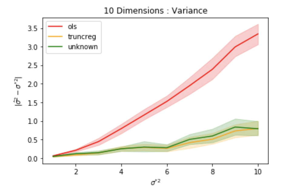
Figure 1: Figure (a) shows w^\hat{w} estimation errors and Figure (b) shows the σ^∗2\hat{\sigma}^{*2} estimation errors for each σ∗2\sigma^{*2}.

In Figure 1, we show how our algorithm performs against models with large noise variances. For this experiment, we sample a 10 dimensional ground-truth weight vector w∗​∼i.i.d.​𝒰​(−1,1)w^{*}\overset{i.i.d.}{\sim}\mathcal{U}(-1,1) and generate 1000010000 (x(i),y(i))(x^{(i)},y^{(i)}) pairs according to x(i)​∼i.i.d.​𝒰​(−5,5)x^{(i)}\overset{i.i.d.}{\sim}\mathcal{U}(-5,5) and y(i)=w∗T​x(i)+ε(i)y^{(i)}={w^{*}}^{T}x^{(i)}+\varepsilon^{(i)}; where ε(i)∼𝒩(0,σ∗2)\varepsilon^{(i)}\sim\mathcal{N}(0,\sigma^{*^{2}}). We fix w∗w^{*} and x(0),…,x(n)x^{(0)},...,x^{(n)} across all trials, but vary σ∗2{\sigma^{*}}^{2}. After adding Gaussian noise to our ground-truth predictions, we left truncate at zero, removing all of the pairs who’s y(i)y^{(i)} is negative; retaining approximately 50%50\% of the original samples. We vary σ∗2\sigma^{*2} over the interval [1,10][1,10] and evaluate how well our procedure recovers w∗w^{*} and σ∗2\sigma^{*2} in comparison to OLS, Daskalakis et al. 2019, given σ∗2\sigma^{*2}, and truncreg, an R package for truncated regression. All three methods

remove a significant amount of bias in the presence of truncation. We emphasize though that truncreg cannot be applied in settings where the truncation is more complicated that a simple interval whereas our method can still be applied.

In Figure 2, we show that our theoretical error bounds hold in practice. For this experiment, we set w∗w^{*} to a ten dimensional weight vector of ones, sample nn (x(i),y(i))(x^{(i)},y^{(i)}) pairs, where x(i)​∼i.i.d.​𝒩​(0,I)x^{(i)}\overset{i.i.d.}{\sim}\mathcal{N}(0,I) and ε(i)​∼i.i.d​𝒩​(0,1)\varepsilon^{(i)}\overset{i.i.d}{\sim}\mathcal{N}(0,1), and right truncate at zero. We generate our data once. However, for each experiment, we randomly select a kk samples that exceed zero, and run our experiment. We vary kk over the interval [10,5000][10,5000]. Our results show that the error bound asymptotically approaches zero at a rate that reaffirms our theoretical analysis.

Refer to caption
Figure 2: Comparison of the proposed method with ordinary least squares.

7 Semi-Synthetic Experiment

Here we show results for an additional experiment that we conducted on semi-synthetic data. For this experiment, we used the Aldrin 2004 dataset. The Aldrin 2004 dataset was originally collected by the Norwegian Public Roads Administration for a study of air pollution at a road in Oslo, Norway. The dataset consists of 500 observations. Interestingly enough, it is common for environmental data to be truncated because of problems in reliably measuring low concentrations.

For this experiment, we apply left truncation to the dataset, varying a truncation parameter CC over the interval [1.0, 4.0]. We run our procedure a total of 10 times and retain the trial that has the smallest gradient as our algorithm’s prediction. We conduct the experiment with the same hyperparameters as for the synthetic data experiments. Below, we report our results.

In Figure 3 (a), we show the L2L^{2} distance between the model parameters of each method and the ground-truth, which we take to be the OLS estimation without truncation. In this figure, we show that our method performs very comparably to Croissant & Zeileis 2018. We also note that, at high values of the truncation, both methods exhibit non-monotonicity in their estimation error, which is presumably due to model misspecification and the truncation being too aggressive.

In Figure 3 (b), we report the L1L^{1} distance between the predicted noise variance and the ground-truth noise variance. Again, our method performs very comparably to Croissant & Zeileis 2018, and we observe non-monotonicity at high values of the truncation.

Refer to caption
(a)
Refer to caption
(b)
Figure 3: Our method’s performance on the semi-synthetic PM10 dataset.

Acknowledgements

CD and PS were supported by NSF Awards CCF-1901292, DMS-2022448 (FODSI) and DMS-2134108, by a Simons Investigator Award, by the Simons Collaboration on the Theory of Algorithmic Fairness, by a DSTA grant, and by the DOE PhILMs project (No. DE-AC05-76RL01830). MZ was supported by NSF DMS-2023505 (FODSI).

References

  • Aldrin (2004) Aldrin, M. Pm10 dataset, 2004. URL http://lib.stat.cmu.edu/datasets/PM10.dat. PM particles at Oslo, Norway.
  • Amemiya (1973) Amemiya, T. Regression analysis when the dependent variable is truncated normal. Econometrica: Journal of the Econometric Society, pp. 997–1016, 1973.
  • Balakrishnan & Cramer (2014) Balakrishnan, N. and Cramer, E. The art of progressive censoring. Springer, 2014.
  • Breen et al. (1996) Breen, R. et al. Regression models: Censored, sample selected, or truncated data, volume 111. Sage, 1996.
  • Carbery & Wright (2001a) Carbery, A. and Wright, J. Distributional and lq̂ norm inequalities for polynomials over convex bodies in rn̂. Mathematical research letters, 8(3):233–248, 2001a.
  • Carbery & Wright (2001b) Carbery, A. and Wright, J. Distributional and Lq{L}^{q} norm inequalities for polynomials over convex bodies in ℝn\mathbb{R}^{n}. Mathematical research letters, 8(3):233–248, 2001b.
  • Croissant & Zeileis (2018) Croissant, Y. and Zeileis, A. truncreg: Estimation of models for truncated gaussian variables by maximum likelihood, 2018. URL https://cran.r-project.org/web/packages/truncreg/truncreg.pdf. R package version 1.8.0.
  • Daskalakis et al. (2018) Daskalakis, C., Gouleakis, T., Tzamos, C., and Zampetakis, M. Efficient statistics, in high dimensions, from truncated samples. In 2018 IEEE 59th Annual Symposium on Foundations of Computer Science (FOCS), pp. 639–649. IEEE, 2018.
  • Daskalakis et al. (2019) Daskalakis, C., Gouleakis, T., Tzamos, C., and Zampetakis, M. Computationally and statistically efficient truncated regression. In Conference on Learning Theory (COLT), pp. 955–960, 2019.
  • Fisher (1931) Fisher, R. Properties and applications of hh functions. Mathematical tables, 1:815–852, 1931.
  • Fotakis et al. (2020) Fotakis, D., Kalavasis, A., and Tzamos, C. Efficient parameter estimation of truncated boolean product distributions. In Conference on Learning Theory, pp. 1586–1600. PMLR, 2020.
  • Galton (1897) Galton, F. An examination into the registered speeds of american trotting horses, with remarks on their value as hereditary data. Proceedings of the Royal Society of London, 62(379-387):310–315, 1897.
  • Hajivassiliou & McFadden (1998) Hajivassiliou, V. A. and McFadden, D. L. The method of simulated scores for the estimation of ldv models. Econometrica, pp. 863–896, 1998.
  • Hausman & Wise (1977) Hausman, J. A. and Wise, D. A. Social experimentation, truncated distributions, and efficient estimation. Econometrica: Journal of the Econometric Society, pp. 919–938, 1977.
  • Heckman (1979) Heckman, J. J. Sample selection bias as a specification error. Econometrica: Journal of the econometric society, pp. 153–161, 1979.
  • Henningsen & Toomet (2011) Henningsen, A. and Toomet, O. maxlik: A package for maximum likelihood estimation in R. Computational Statistics, 26(3):443–458, 2011. doi: 10.1007/s00180-010-0217-1. URL http://dx.doi.org/10.1007/s00180-010-0217-1.
  • Ilyas et al. (2020) Ilyas, A., Zampetakis, E., and Daskalakis, C. A theoretical and practical framework for regression and classification from truncated samples. In International Conference on Artificial Intelligence and Statistics, pp. 4463–4473. PMLR, 2020.
  • Kontonis et al. (2019) Kontonis, V., Tzamos, C., and Zampetakis, M. Efficient truncated statistics with unknown truncation. In 2019 IEEE 60th Annual Symposium on Foundations of Computer Science (FOCS), pp. 1578–1595. IEEE, 2019.
  • Leluc & Portier (2020) Leluc, R. and Portier, F. Towards asymptotic optimality with conditioned stochastic gradient descent. arXiv preprint arXiv:2006.02745, 2020.
  • Mohan et al. (2013) Mohan, K., Pearl, J., and Tian, J. Graphical models for inference with missing data. In Proceedings of the 26th Annual Conference on Neural Information Processing Systems (NeurIPS), 2013.
  • Moitra et al. (2021) Moitra, A., Mossel, E., and Sandon, C. Learning to sample from censored markov random fields. arXiv preprint arXiv:2101.06178, 2021.
  • Pearson (1902) Pearson, K. On the systematic fitting of frequency curves. Biometrika, 2:2–7, 1902.
  • Pearson & Lee (1908) Pearson, K. and Lee, A. On the generalised probable error in multiple normal correlation. Biometrika, 6(1):59–68, 1908.
  • Plevrakis (2021) Plevrakis, O. Learning from censored and dependent data: The case of linear dynamics. Conference on Learning Theory – COLT, 2021.
  • Rakhlin et al. (2011) Rakhlin, A., Shamir, O., and Sridharan, K. Making gradient descent optimal for strongly convex stochastic optimization. arXiv preprint arXiv:1109.5647, 2011.
  • Shamir & Zhang (2013) Shamir, O. and Zhang, T. Stochastic gradient descent for non-smooth optimization: Convergence results and optimal averaging schemes. In International conference on machine learning, pp. 71–79. PMLR, 2013.
  • Tobin (1958) Tobin, J. Estimation of relationships for limited dependent variables. Econometrica: journal of the Econometric Society, pp. 24–36, 1958.
  • Tropp (2015) Tropp, J. A. An introduction to matrix concentration inequalities. arXiv preprint arXiv:1501.01571, 2015.
  • Tukey (1949) Tukey, J. W. Sufficiency, truncation and selection. The Annals of Mathematical Statistics, pp. 309–311, 1949.

Appendix A Projection Set

If it is not specified, all the norms for vectors are L2L^{2} norms, by default.

A.1 Proof for the convexity of the projection set

Recall that the projection set is

Dr={(v,λ)=(wσ2,1σ2)∈ℝk×ℝ|18​(5−2​log⁡a)≤σ2σ02≤96a2,‖w‖22≤β}\displaystyle D_{r}=\left\{(v,\lambda)=\left({w\over\sigma^{2}},{1\over\sigma^{2}}\right)\in\mathbb{R}^{k}\times\mathbb{R}\penalty\ \Big|\penalty\ \frac{1}{8(5-2\log a)}\leq\frac{{\sigma}^{2}}{\sigma_{0}^{2}}\leq\frac{96}{a^{2}},\left\lVert w\right\rVert_{2}^{2}\leq\beta\right\}

So we have

‖w‖2=wT​w=(v/λ)T​(v/λ)=vT​v/λ2=‖v‖2/λ2\left\lVert w\right\rVert^{2}=w^{T}w=(v/\lambda)^{T}(v/\lambda)=v^{T}v/\lambda^{2}=\left\lVert v\right\rVert^{2}/\lambda^{2}

Therefore, if we transform it into a direct representation with v,λv,\lambda, we get

Dr={(v,λ)∈ℝk×ℝ>0|a296​σ02≤λ≤8​(5−2​log⁡a)σ02,‖v‖2≤βλ2}D_{r}=\left\{(v,\lambda)\in\mathbb{R}^{k}\times\mathbb{R}_{>0}\penalty\ \Big|\penalty\ \frac{a^{2}}{96\sigma_{0}^{2}}\leq\lambda\leq\frac{8(5-2\log a)}{\sigma_{0}^{2}},\left\lVert v\right\rVert^{2}\leq\beta\lambda^{2}\right\}

Where ℝ>0\mathbb{R}_{>0} denotes the set of positive real numbers. We prove that this is a convex set by showing that it is an (infinite) intersection of convex sets.

The first constraint a296​σ02≤λ≤8​(5−2​log⁡a)σ02\frac{a^{2}}{96\sigma_{0}^{2}}\leq\lambda\leq\frac{8(5-2\log a)}{\sigma_{0}^{2}} is a region between two hyper planes, which is also a convex constraint.

We prove that the second constraint ‖v‖2≤β​λ2\left\lVert v\right\rVert^{2}\leq\beta\lambda^{2} is convex. Suppose we have two vectors such that ‖v1‖2≤β​λ12\left\lVert v_{1}\right\rVert^{2}\leq\beta\lambda_{1}^{2} and ‖v2‖2≤β​λ22\left\lVert v_{2}\right\rVert^{2}\leq\beta\lambda_{2}^{2}. We need to prove that ‖μ​v1+(1−μ)​v2‖2≤β​(μ​λ1+(1−μ)​λ2)2\left\lVert\mu v_{1}+(1-\mu)v_{2}\right\rVert^{2}\leq\beta(\mu\lambda_{1}+(1-\mu)\lambda_{2})^{2} for all μ∈(0,1)\mu\in(0,1). With this condition and knowing that λ1,λ2>0\lambda_{1},\lambda_{2}>0, we know that ‖v1‖≤β​λ1\left\lVert v_{1}\right\rVert\leq\sqrt{\beta}\lambda_{1} and ‖v2‖≤β​λ2\left\lVert v_{2}\right\rVert\leq\sqrt{\beta}\lambda_{2}. By the triangle inequality, we have ‖μ​v1+(1−μ)​v2‖2≤(μ⁡‖v1‖+(1−μ)​‖v2‖)2≤(μ​β​λ1+(1−μ)​β​λ2)2=β​(μ​λ1+(1−μ)​λ2)2\left\lVert\mu v_{1}+(1-\mu)v_{2}\right\rVert^{2}\leq(\mu\left\lVert v_{1}\right\rVert+(1-\mu)\left\lVert v_{2}\right\rVert)^{2}\leq(\mu\sqrt{\beta}\lambda_{1}+(1-\mu)\sqrt{\beta}\lambda_{2})^{2}=\beta(\mu\lambda_{1}+(1-\mu)\lambda_{2})^{2}. So, we proved the convexity of the third constraint.

Since the three constraints are all convex and the projection set is the intersection of the three constraints, the projection set is convex.

A.2 Algorithm for projecting to the projection set

We have an explicit formula for projecting to the projection set. For convenience, we denote λmin=a296​σ02\lambda_{\min}=\frac{a^{2}}{96\sigma_{0}^{2}} and λmax=8​(5−2​log⁡a)σ02\lambda_{\max}=\frac{8(5-2\log a)}{\sigma_{0}^{2}}. Thus, the projection formula projects (v,λ)∈Dr(v,\lambda)\in D_{r} by minimizing ‖(v0,λ0)−(v,λ)‖\left\lVert(v_{0},\lambda_{0})-(v,\lambda)\right\rVert) as below:

{(v0,λ0)λmin≤λ0≤λmax,‖v0‖2≤β​λ02(v0,λmax)λ0≥λmax,‖v0‖2≤β​λmax2(β​λmax‖v0‖​v0,λmax)λ0≥λmax,‖v0‖2≥β​λmax2(v0,λmin)λ0≤λmin,‖v0‖2≤β​λmin2(β​λmin‖v0‖​v0,λmin)λ0≤λmin,β​λmin≤‖v0‖≤β​λmin+λmin−λ0β(β​λmax‖v0‖​v0,λmax)λ0≤λmax,‖v0‖≥β​λmax+λmax−λ0β(β⁡‖v0‖+β​λ0(β+1)​‖v0‖​v0,β​‖v0‖+λ0β+1)Otherwise\left\{\begin{array}[]{cc}(v_{0},\lambda_{0})&\lambda_{\min}\leq\lambda_{0}\leq\lambda_{\max},\penalty\ \left\lVert v_{0}\right\rVert^{2}\leq\beta\lambda_{0}^{2}\\ (v_{0},\lambda_{\max})&\lambda_{0}\geq\lambda_{\max},\penalty\ \left\lVert v_{0}\right\rVert^{2}\leq\beta\lambda_{\max}^{2}\\ \left(\frac{\sqrt{\beta}\lambda_{\max}}{\left\lVert v_{0}\right\rVert}v_{0},\lambda_{\max}\right)&\lambda_{0}\geq\lambda_{\max},\penalty\ \left\lVert v_{0}\right\rVert^{2}\geq\beta\lambda_{\max}^{2}\\ (v_{0},\lambda_{\min})&\lambda_{0}\leq\lambda_{\min},\penalty\ \left\lVert v_{0}\right\rVert^{2}\leq\beta\lambda_{\min}^{2}\\ \left(\frac{\sqrt{\beta}\lambda_{\min}}{\left\lVert v_{0}\right\rVert}v_{0},\lambda_{\min}\right)&\lambda_{0}\leq\lambda_{\min},\penalty\ \sqrt{\beta}\lambda_{\min}\leq\left\lVert v_{0}\right\rVert\leq\sqrt{\beta}\lambda_{\min}+\frac{\lambda_{\min}-\lambda_{0}}{\sqrt{\beta}}\\ \left(\frac{\sqrt{\beta}\lambda_{\max}}{\left\lVert v_{0}\right\rVert}v_{0},\lambda_{\max}\right)&\lambda_{0}\leq\lambda_{\max},\penalty\ \left\lVert v_{0}\right\rVert\geq\sqrt{\beta}\lambda_{\max}+\frac{\lambda_{\max}-\lambda_{0}}{\sqrt{\beta}}\\ \left(\frac{\beta\left\lVert v_{0}\right\rVert+\sqrt{\beta}\lambda_{0}}{(\beta+1)\left\lVert v_{0}\right\rVert}v_{0},\frac{\sqrt{\beta}\left\lVert v_{0}\right\rVert+\lambda_{0}}{\beta+1}\right)&\text{Otherwise}\\ \end{array}\right.

Appendix B Missing Proofs

If it is not specified, all the norms for vectors are L2L^{2} norms, by default.

B.1 Sampling the Gradient of the Objective Function

Let 𝒟∗\mathcal{D}^{*} be the joint distribution of the observed pairs (x,y)(x,y), where (w∗,σ∗)(w^{*},\sigma^{*}) are the ground truth parameters. Notice that we have a sampler that generates samples (x,y)(x,y) from D∗D^{*}. Also let’s define 𝒟(w,σ)\mathcal{D}_{(w,\sigma)} as the joint distribution of the pairs (x,y)(x,y), when the vector of parameters is (w,σ)(w,\sigma). We recall that 𝒫\mathcal{P} is the marginal distribution of xx of the joint distribution 𝒟∗\mathcal{D}^{*}. Also, 𝒫0\mathcal{P}_{0} is the original distribution of xx before truncation.

So, after truncation, we have

𝒟∗​(x¯,y¯)=𝟏{y¯∈S}⋅𝒩(w∗Tx¯,σ∗2;y¯)⋅𝒫0(x¯)𝔼x∼𝒫0[α(w∗,σ∗,x¯;S))]\mathcal{D}^{*}(\bar{x},\bar{y})=\frac{\mathbf{1}\{\bar{y}\in S\}\cdot\mathcal{N}(w^{*T}\bar{x},\sigma^{*2};\bar{y})\cdot\mathcal{P}_{0}(\bar{x})}{\Exp_{x\sim\mathcal{P}_{0}}\left[\alpha(w^{*},\sigma^{*},\bar{x};S))\right]}

We note that 𝒩⁡(w∗T​x¯,σ∗2,y¯)\mathcal{N}(w^{*T}\bar{x},\sigma^{*2};\bar{y}) is the probability density of y¯\bar{y}; that is, exp⁡(−(y¯−w∗T​x)22​σ∗2)\exp\left({-\frac{(\bar{y}-w^{*T}x)^{2}}{2{\sigma^{*}}^{2}}}\right). To make it explicit, let’s say that the relationship between 𝒫\mathcal{P} and 𝒫0\mathcal{P}_{0} is,

𝒫⁡(x¯)=∫ℝ𝟏{y¯∈S}⋅𝒩(w∗Tx¯,σ∗2;y¯)⋅𝒫0(x¯)𝔼x∼𝒫0[α⁡(w∗,σ∗,x¯,S)]​𝑑y¯=α⁡(w∗,σ∗,x¯,S)𝔼x∼𝒫0[α(w∗,σ∗,x¯;S))]⋅𝒫0​(x¯)\mathcal{P}(\bar{x})=\int_{\mathbb{R}}\frac{\mathbf{1}\{\bar{y}\in S\}\cdot\mathcal{N}(w^{*T}\bar{x},\sigma^{*2};\bar{y})\cdot\mathcal{P}_{0}(\bar{x})}{\Exp_{x\sim\mathcal{P}_{0}}\left[\alpha(w^{*},\sigma^{*},\bar{x};S)\right]}d\bar{y}=\frac{\alpha(w^{*},\sigma^{*},\bar{x};S)}{\Exp_{x\sim\mathcal{P}_{0}}\left[\alpha(w^{*},\sigma^{*},\bar{x};S))\right]}\cdot\mathcal{P}_{0}(\bar{x})

Now we can sample the gradient. The gradient is

∂ℓ¯∂v=𝔼x∼𝒫[𝔼z∼Qx[z⋅x]−𝔼y∼Fx[y⋅x]]∂ℓ¯∂λ=12​𝔼x∼𝒫[𝔼y∼Fx[y2]−𝔼z∼Qx[z2]],\frac{\partial\bar{\ell}}{\partial v}=\Exp_{x\sim\mathcal{P}}\left[\Exp_{z\sim Q_{x}}\left[z\cdot x\right]-\Exp_{y\sim F_{x}}\left[y\cdot x\right]\right]\penalty\ \penalty\ \penalty\ \penalty\ \frac{\partial\bar{\ell}}{\partial\lambda}=\frac{1}{2}\Exp_{x\sim\mathcal{P}}\left[\Exp_{y\sim F_{x}}\left[y^{2}\right]-\Exp_{z\sim Q_{x}}\left[z^{2}\right]\right],

Where Fx=𝒩⁡(w∗T​x,σ∗2,S)F_{x}=\mathcal{N}({w^{*}}^{T}x,{\sigma^{*}}^{2},S) and Qx=𝒩⁡(wT​x,σ2,S)Q_{x}=\mathcal{N}({w}^{T}x,{\sigma}^{2},S). Further, note that

𝔼x∼𝒫[𝔼y∼𝒩⁡(w∗T​x,σ∗2,S)[y⋅x]]\displaystyle\penalty\ \penalty\ \penalty\ \penalty\ \Exp_{x\sim\mathcal{P}}\left[\Exp_{y\sim\mathcal{N}(w^{*T}x,\sigma^{*2},S)}\left[y\cdot x\right]\right]
=∫x∫S(y⋅x)​𝒩⁡(w∗T​x,σ∗2,y¯)𝒩⁡(w∗T​x,σ∗2,S)⋅𝑑y⋅𝒫⁡(x)⋅𝑑x\displaystyle=\int_{x}\int_{S}(y\cdot x)\frac{\mathcal{N}(w^{*T}x,\sigma^{*2};\bar{y})}{\mathcal{N}(w^{*T}x,\sigma^{*2};S)}\cdot dy\cdot\mathcal{P}(x)\cdot dx
=∫x∫S(y⋅x)​𝒩⁡(w∗T​x,σ∗2,y¯)𝒩⁡(w∗T​x,σ∗2,S)⋅𝑑y⋅𝒩⁡(w∗T​x¯,σ∗2,S)𝔼x∼𝒫0[𝒩⁡(w∗T​x,σ∗2,S)]⋅𝒫0​(x¯)⋅𝑑x\displaystyle=\int_{x}\int_{S}(y\cdot x)\frac{\mathcal{N}(w^{*T}x,\sigma^{*2};\bar{y})}{\mathcal{N}(w^{*T}x,\sigma^{*2};S)}\cdot dy\cdot\frac{\mathcal{N}(w^{*T}\bar{x},\sigma^{*2};S)}{\Exp_{x\sim\mathcal{P}_{0}}\left[\mathcal{N}(w^{*T}x,\sigma^{*2};S)\right]}\cdot\mathcal{P}_{0}(\bar{x})\cdot dx
=∫x∫S(y⋅x)​𝒩⁡(w∗T​x,σ∗2,y¯)𝔼x∼𝒫0[𝒩⁡(w∗T​x,σ∗2,S)]⋅𝒫0​(x¯)⋅𝑑y⋅𝑑x=𝔼(x,y)∼𝒟∗[y⋅x]\displaystyle=\int_{x}\int_{S}(y\cdot x)\frac{\mathcal{N}(w^{*T}x,\sigma^{*2};\bar{y})}{\Exp_{x\sim\mathcal{P}_{0}}\left[\mathcal{N}(w^{*T}x,\sigma^{*2};S)\right]}\cdot\mathcal{P}_{0}(\bar{x})\cdot dy\cdot dx=\Exp_{(x,y)\sim\mathcal{D}^{*}}\left[y\cdot x\right]

At each gradient step, we sample a pair of x,yx,y and multiply them together. Similarly we sample 12​y2\frac{1}{2}y^{2}, where x∼𝒫x\sim\mathcal{P} and y∼Fxy\sim F_{x}, and ignore xx after sampling. For the second term, we use rejection sampling to generate the data z⋅xz\cdot x for z∼Qxz\sim Q_{x} and x∼𝒫x\sim\mathcal{P}. Here, since we know the ww and σ\sigma, the generation process is simple. First, we generate xx using 𝒟∗\mathcal{D}^{*} (we discard the yy value) and then sample z=wT​x+εz=w^{T}x+\varepsilon where ε=𝒩⁡(0,σ2)\varepsilon=\mathcal{N}(0,\sigma^{2}). If z∉Sz\notin S, we continue to sample ε\varepsilon until we get z∈Sz\in S. Similarly, we can sample 12​z2\frac{1}{2}z^{2} where x∼𝒫,z∼Qxx\sim\mathcal{P},z\sim Q_{x} in this way, and we can ignore xx after sampling.

Notice that if w,σ=w∗,σ∗w,\sigma=w^{*},\sigma^{*}, we have Qx=FxQ_{x}=F_{x}, so

∂ℓ¯∂v​(w∗T,σ∗2)=𝔼x∼𝒫[𝔼z∼Qx[z⋅x]−𝔼y∼Fx[y⋅x]]=0\frac{\partial\bar{\ell}}{\partial v}(w^{*T},\sigma^{*2})=\Exp_{x\sim\mathcal{P}}\left[\Exp_{z\sim Q_{x}}\left[z\cdot x\right]-\Exp_{y\sim F_{x}}\left[y\cdot x\right]\right]=0

and

∂ℓ¯∂λ=12​𝔼x∼𝒫[𝔼y∼Fx[y2]−𝔼z∼Qx[z2]]=0.\frac{\partial\bar{\ell}}{\partial\lambda}=\frac{1}{2}\Exp_{x\sim\mathcal{P}}\left[\Exp_{y\sim F_{x}}\left[y^{2}\right]-\Exp_{z\sim Q_{x}}\left[z^{2}\right]\right]=0.

B.2 Auxilliary Lemmas for Survival Probability of Feasible Points

For many of the following proofs, we require an estimation of α⁡(w,σ,x)\alpha(w,\sigma,x) for a feasible ww.

Lemma B.1.

Let x,w,w′∈ℝkx,w,w^{\prime}\in\mathbb{R}^{k} and σ,σ′>0\sigma,\sigma^{\prime}>0. Then,

log⁡(1α⁡(w,σ,x))≤max⁡(1,2​σ′2σ2)​log⁡1α⁡(w′,σ′,x)+max⁡(0,4​σ′2σ2−2)+2​σ′2σ2​((wT​x−w′T​x)22​σ′2)\displaystyle\log\left(\frac{1}{\alpha(w,\sigma,x)}\right)\leq\max\left(1,\frac{2{\sigma^{\prime}}^{2}}{\sigma^{2}}\right)\log\frac{1}{\alpha(w^{\prime},\sigma^{\prime},x)}+\max\left(0,\frac{4{\sigma^{\prime}}^{2}}{\sigma^{2}}-2\right)+\frac{2{\sigma^{\prime}}^{2}}{\sigma^{2}}\left(\frac{(w^{T}x-{w^{\prime}}^{T}x)^{2}}{2{\sigma^{\prime}}^{2}}\right)
Proof.

Now, let’s define DD, D′D^{\prime}, and DS′D^{\prime}_{S} as D=𝒩⁡(wT​x,σ)D=\mathcal{N}(w^{T}x,\sigma), D′=𝒩⁡(w′T​x,σ′)D^{\prime}=\mathcal{N}(w^{\prime T}x,\sigma^{\prime}), and DS′=𝒩⁡(w′T​x,σ′,S)D^{\prime}_{S}=\mathcal{N}(w^{\prime T}x,\sigma^{\prime},S). Then, we have:

α⁡(w,σ,x)=𝔼y∼D[𝟏y∈S]=\displaystyle\alpha(w,\sigma,x)=\Exp_{y\sim D}\Big[{\mathbf{1}_{y\in S}}\Big]= 𝔼y∼D′[𝟏y∈S​exp⁡((y−w′T​x)22​σ′2−(y−wT​x)22​σ2)]\displaystyle\Exp_{y\sim D^{\prime}}\Bigg[{\mathbf{1}_{y\in S}}\exp\left(\frac{(y-w^{\prime T}x)^{2}}{2\sigma^{\prime 2}}-\frac{(y-w^{T}x)^{2}}{2\sigma^{2}}\right)\Bigg]
=\displaystyle= α⁡(w′,σ′,x)⋅𝔼y∼DS′[exp⁡((y−w′T​x)22​σ′2−(y−wT​x)22​σ2)]\displaystyle\alpha(w^{\prime},\sigma^{\prime},x)\cdot\Exp_{y\sim D^{\prime}_{S}}\Bigg[\exp\left(\frac{(y-w^{\prime T}x)^{2}}{2\sigma^{\prime 2}}-\frac{(y-w^{T}x)^{2}}{2\sigma^{2}}\right)\Bigg]
≥\displaystyle\geq α⁡(w′,σ′,x)⋅exp⁡(𝔼y∼DS′[(y−w′T​x)22​σ′2−(y−wT​x)22​σ2]).\displaystyle\alpha(w^{\prime},\sigma^{\prime},x)\cdot\exp\left(\Exp_{y\sim D^{\prime}_{S}}\Bigg[\frac{(y-w^{\prime T}x)^{2}}{2\sigma^{\prime 2}}-\frac{(y-w^{T}x)^{2}}{2\sigma^{2}}\Bigg]\right).

Now, from Cauchy-Schwarz we have that

(y−wT​x)22​σ2≤2​σ′2σ2​((y−w′T​x)22​σ′2+(wT​x−w′T​x)22​σ′2)\displaystyle\frac{(y-w^{T}x)^{2}}{2\sigma^{2}}\leq\frac{2{\sigma^{\prime}}^{2}}{\sigma^{2}}\left(\frac{(y-{w^{\prime}}^{T}x)^{2}}{2{\sigma^{\prime}}^{2}}+\frac{(w^{T}x-{w^{\prime}}^{T}x)^{2}}{2{\sigma^{\prime}}^{2}}\right)

and if we apply this to the above expression and take the logarithm of both sides of the inequality we get

log⁡α⁡(w,σ,x)\displaystyle\log\alpha(w,\sigma,x)
≥\displaystyle\geq log⁡α⁡(w′,σ′,x)+𝔼y∼DS′[(1−2​σ′2σ2)​(y−w′T​x)22​σ′2]−𝔼y∼DS′[2​σ′2σ2​((wT​x−w′T​x)22​σ′2)]\displaystyle\log\alpha(w^{\prime},\sigma^{\prime},x)+\Exp_{y\sim D^{\prime}_{S}}\Bigg[\left(1-\frac{2{\sigma^{\prime}}^{2}}{\sigma^{2}}\right)\frac{(y-w^{\prime T}x)^{2}}{2\sigma^{\prime 2}}\Bigg]-\Exp_{y\sim D^{\prime}_{S}}\Bigg[\frac{2{\sigma^{\prime}}^{2}}{\sigma^{2}}\left(\frac{(w^{T}x-{w^{\prime}}^{T}x)^{2}}{2{\sigma^{\prime}}^{2}}\right)\Bigg]
≥\displaystyle\geq log⁡α⁡(w′,σ′,x)+𝔼y∼DS′[min⁡(0,1−2​σ′2σ2)​(2−log⁡α⁡(w′,σ′,x))−2​σ′2σ2​((wT​x−w′T​x)22​σ′2)]\displaystyle\log\alpha(w^{\prime},\sigma^{\prime},x)+\Exp_{y\sim D^{\prime}_{S}}\Bigg[\min\left(0,1-\frac{2{\sigma^{\prime}}^{2}}{\sigma^{2}}\right)(2-\log\alpha(w^{\prime},\sigma^{\prime},x))-\frac{2{\sigma^{\prime}}^{2}}{\sigma^{2}}\left(\frac{(w^{T}x-{w^{\prime}}^{T}x)^{2}}{2{\sigma^{\prime}}^{2}}\right)\Bigg]
=\displaystyle= min⁡(−1,−2​σ′2σ2)​(−log⁡α⁡(w′,σ′,x))−min⁡(0,2−4​σ′2σ2)−2​σ′2σ2​((wT​x−w′T​x)22​σ′2)\displaystyle\min\left(-1,-\frac{2{\sigma^{\prime}}^{2}}{\sigma^{2}}\right)(-\log\alpha(w^{\prime},\sigma^{\prime},x))-\min\left(0,2-\frac{4{\sigma^{\prime}}^{2}}{\sigma^{2}}\right)-\frac{2{\sigma^{\prime}}^{2}}{\sigma^{2}}\left(\frac{(w^{T}x-{w^{\prime}}^{T}x)^{2}}{2{\sigma^{\prime}}^{2}}\right)

The second to last line is followed from Lemma 4.5 and the Lemma follows. ∎

B.3 Proof of Theorem 4.1 and Lemma 4.4

Denote s=maxσ∈D⁡σminσ∈D⁡σ=8​(5−2​log⁡a)​96a2s=\frac{\max_{\sigma\in D}\sigma}{\min_{\sigma\in D}\sigma}=\sqrt{8(5-2\log a)\frac{96}{a^{2}}} be the largest possible difference between variances, where DD is the projection set defined in 3.1.

Next, to prove our strong convexity result, we use the following anti-concentration bound.

Theorem B.2 (Theorem 8 in [6])).

There is an absolute constant 𝒞\mathcal{C} such that if p:ℝn→ℝp:\mathbb{R}^{n}\to\mathbb{R} is a polynomial of degree at most dd, 0<q<∞0<q<\infty, and μ\mu is a log-concave probability measure on ℝn\mathbb{R}^{n}, then

(∫|p(x)|q/ddμ(x))1/qα−1/d⋅μ{x∈ℝn:|p(x)|≤α}≤𝒞q\displaystyle\left(\int|p(x)|^{q/d}\mathrm{d}\mu(x)\right)^{1/q}\alpha^{-1/d}\cdot\mu\left\{x\in\mathbb{R}^{n}:|p(x)|\leq\alpha\right\}\leq\mathcal{C}q

We also need the following lemma for bounding the survival probability for any parameters in DD.

Lemma B.3.

For w,σ∈Dw,\sigma\in D, we can find a lower bound for the survival probability: 1α⁡(w,σ,x(i))≤exp⁡(poly⁡(1/a)​(1+βσ02))\frac{1}{\alpha(w,\sigma,x^{(i)})}\leq\exp(\mathrm{poly}(1/a)(1+\frac{\beta}{\sigma_{0}^{2}}))

Proof.

From Lemma B.1, when we plug σ′=σ∗,w′=w∗\sigma^{\prime}=\sigma^{*},w^{\prime}=w^{*}, we can derive that

log⁡(1α⁡(w,σ,x))≤\displaystyle\log\left(\frac{1}{\alpha(w,\sigma,x)}\right)\leq max⁡(1,2​σ∗2σ2)​log⁡(1α⁡(w∗,σ∗,x))\displaystyle\max\left(1,\frac{2{\sigma^{*}}^{2}}{\sigma^{2}}\right)\log\left(\frac{1}{\alpha(w^{*},\sigma^{*},x)}\right)
+\displaystyle+ max⁡(0,4​σ∗2σ2−2)+2​σ∗2σ2​((wT​x−w∗T​x)22​σ∗2)\displaystyle\max\left(0,\frac{4{\sigma^{*}}^{2}}{\sigma^{2}}-2\right)+\frac{2{\sigma^{*}}^{2}}{\sigma^{2}}\left(\frac{(w^{T}x-{w^{*}}^{T}x)^{2}}{2{\sigma^{*}}^{2}}\right)

Since σ,σ∗∈D\sigma,\sigma^{*}\in D, we have σ∗2σ2≤s2\frac{{\sigma^{*}}^{2}}{\sigma^{2}}\leq s^{2}. Thus, we have

log⁡(1α⁡(w,σ,x))\displaystyle\log\left(\frac{1}{\alpha(w,\sigma,x)}\right)
≤\displaystyle\leq max⁡(1,2​σ∗2σ2)​log⁡(1α⁡(w∗,σ∗,x))+max⁡(0,4​σ∗2σ2−2)+2​σ∗2σ2​((wT​x−w∗T​x)22​σ∗2)\displaystyle\max\left(1,\frac{2{\sigma^{*}}^{2}}{\sigma^{2}}\right)\log\left(\frac{1}{\alpha(w^{*},\sigma^{*},x)}\right)+\max\left(0,\frac{4{\sigma^{*}}^{2}}{\sigma^{2}}-2\right)+\frac{2{\sigma^{*}}^{2}}{\sigma^{2}}\left(\frac{(w^{T}x-{w^{*}}^{T}x)^{2}}{2{\sigma^{*}}^{2}}\right)
≤\displaystyle\leq 2​s2​(log⁡1α⁡(w∗,σ∗,x)+2+((wT​x−w∗T​x)22​σ∗2))\displaystyle 2s^{2}\left(\log\frac{1}{\alpha(w^{*},\sigma^{*},x)}+2+\left(\frac{(w^{T}x-{w^{*}}^{T}x)^{2}}{2{\sigma^{*}}^{2}}\right)\right)
≤\displaystyle\leq 2​s2​(−log⁡a+2+((‖w‖2+‖w∗‖2)​‖x‖2σ∗2))\displaystyle 2s^{2}\left(-\log a+2+\left(\frac{(\left\lVert w\right\rVert^{2}+\left\lVert w^{*}\right\rVert^{2})\left\lVert x\right\rVert^{2}}{{\sigma^{*}}^{2}}\right)\right)
≤\displaystyle\leq 2​s2​(−log⁡a+2+(2​βσ∗2))\displaystyle 2s^{2}\left(-\log a+2+\left(\frac{2\beta}{{\sigma^{*}}^{2}}\right)\right)

Since σ0\sigma_{0} and σ∗\sigma^{*} only have a polynomial difference, we have log⁡(1α⁡(w,σ,x))≤poly⁡(1/a)​(1+βσ02)\log\Big(\frac{1}{\alpha(w,\sigma,x)}\Big)\leq\mathrm{poly}(1/a)(1+\frac{\beta}{\sigma_{0}^{2}}) which finishes the proof. ∎

Lemma B.4.

Let z∼𝒩⁡(μ,σ2,S)z\sim\mathcal{N}(\mu,\sigma^{2},S) be a truncated normal variable. Assume α⁡(μ,σ2,S)=a\alpha(\mu,\sigma^{2},S)=a. Then, we have that

Var⁡(z2)=2​μ2​σ2​(O⁡(log⁡(a)))+σ4​O​(log⁡(a)2)\mathrm{Var}(z^{2})=2\mu^{2}\sigma^{2}(O(\log(a)))+\sigma^{4}O(\log(a)^{2})
Proof.

Denote an affine transformation S′={x−μσ|x∈S}S^{\prime}=\{\frac{x-\mu}{\sigma}|x\in S\}. So D=𝒩⁡(μ,σ,S)D=\mathcal{N}(\mu,\sigma,S) is transformed into D′=𝒩⁡(0,1,S′)D^{\prime}=\mathcal{N}(0,1,S^{\prime}), while the survival probability is maintained. We then have

Varz∼D​(z2)\displaystyle\mathrm{Var}_{z\sim D}(z^{2}) =Vary∼D′​((μ+σ​y)2)=Vary∼D′​(2​σ​μ​y+σ2​y2)\displaystyle=\mathrm{Var}_{y\sim D^{\prime}}((\mu+\sigma y)^{2})=\mathrm{Var}_{y\sim D^{\prime}}(2\sigma\mu y+\sigma^{2}y^{2})
≤8​(σ​μ)2​Vary∼D′​(y)+2​(σ)4​Vary∼D′​(y2)\displaystyle\leq 8(\sigma\mu)^{2}\mathrm{Var}_{y\sim D^{\prime}}(y)+2(\sigma)^{4}\mathrm{Var}_{y\sim D^{\prime}}(y^{2})

By Lemma 4.5 we have Vary∼D′​[y]≤𝔼⁡[y2]≤4−2​log⁡a\mathrm{Var}_{y\sim D^{\prime}}[y]\leq\mathbb{E}[y^{2}]\leq 4-2\log a, and

VarD′​(y2)≤𝔼D′​(y4)≤∫q∞x4​e−x22​𝑑x∫q∞e−x22​𝑑x=∫q∞x4​e−x22​𝑑xa/2\displaystyle\mathrm{Var}_{D^{\prime}}(y^{2})\leq\mathbb{E}_{D^{\prime}}(y^{4})\leq\frac{\int_{q}^{\infty}x^{4}e^{-\frac{x^{2}}{2}}\mathrm{d}x}{\int_{q}^{\infty}e^{-\frac{x^{2}}{2}}\mathrm{d}x}=\frac{\int_{q}^{\infty}x^{4}e^{-\frac{x^{2}}{2}}\mathrm{d}x}{a/2}

where qq satisfies ∫q∞e−x22​𝑑x=a/2\int_{q}^{\infty}e^{-\frac{x^{2}}{2}}\mathrm{d}x=a/2.

Now, all we need to prove is that q=O⁡(−log⁡a)q=O(\sqrt{-\log a}). Notice that if q>2​−log⁡aq>2\sqrt{-\log a} (in the case a<2/2a<\sqrt{2}/2 and q>1q>1), then we have

a/2=\displaystyle a/2= ∫q∞e−z2/2dz=∫q2/2∞1ze−zdz<2qe−q2/2<2a2/q<a\displaystyle\int_{q}^{\infty}e^{-z^{2}/2}\mathrm{d}z=\int_{q^{2}/2}^{\infty}\frac{1}{\sqrt{z}}e^{-z}\mathrm{d}z<\frac{\sqrt{2}}{q}e^{-q^{2}/2}<\sqrt{2}a^{2}/q<a

This is a contradiction.

By integration by parts, we obtain

∫q∞z4e−z2/2dz=q3e−q2/2+3∫q∞z2e−z2/2dz=q3e−q2/2+3qe−q2/2+3∫q∞e−z2/2dz\displaystyle{\int_{q}^{\infty}z^{4}e^{-z^{2}/2}\mathrm{d}z}=q^{3}e^{-q^{2}/2}+3{\int_{q}^{\infty}z^{2}e^{-z^{2}/2}\mathrm{d}z}=q^{3}e^{-q^{2}/2}+3qe^{-q^{2}/2}+3\int_{q}^{\infty}e^{-z^{2}/2}\mathrm{d}z

and

∫q∞z4e−z2/2dz∫q∞e−z2/2dz=3+q3e−q2/2+3qe−q2/2∫q∞e−z2/2dz≤3+q3e−q2/2+3qe−q2/2∫qq+1/qe−(q2+3)/2dz≤3+15​q2+5​q4\displaystyle\frac{\int_{q}^{\infty}z^{4}e^{-z^{2}/2}\mathrm{d}z}{\int_{q}^{\infty}e^{-z^{2}/2}\mathrm{d}z}=3+\frac{q^{3}e^{-q^{2}/2}+3qe^{-q^{2}/2}}{\int_{q}^{\infty}e^{-z^{2}/2}\mathrm{d}z}\leq 3+\frac{q^{3}e^{-q^{2}/2}+3qe^{-q^{2}/2}}{\int_{q}^{q+1/q}e^{-(q^{2}+3)/2}\mathrm{d}z}\leq 3+15q^{2}+5q^{4}

Since when a<2/2a<\sqrt{2}/2, we have both q<2​−log⁡aq<2\sqrt{-\log a} and VarD​s′​(y2)=O⁡(log⁡a2)\mathrm{Var}_{Ds^{\prime}}(y^{2})=O(\log a^{2}). The lemma follows. ∎

B.3.1 Strong Convexity

Now, let’s deal with the Hessian Matrix.

First, we consider the case without truncation, that is,

𝔼𝒫​[(Varx​[z]​x​xT−Covx​[12​z2,z]​x−Covx​[12​z2,z]​xTVarx​[12​z2])]\mathbb{E}_{\mathcal{P}}\left[\begin{pmatrix}\mathrm{Var}_{x}[z]xx^{T}&-\mathrm{Cov}_{x}\Big[\frac{1}{2}z^{2},z\Big]x\\ -\mathrm{Cov}_{x}\Big[\frac{1}{2}z^{2},z\Big]{x}^{T}&\mathrm{Var}_{x}\Big[\frac{1}{2}z^{2}\Big]\end{pmatrix}\right]

The variance (Varx\text{Var}_{x}) and covariance (Covx\text{Cov}_{x}) are calculated from the untruncated normal z∼𝒩⁡(wT​x,σ2)z\sim\mathcal{N}(w^{T}x,\sigma^{2}). For all xx, we have

(vλ)T​(Varx​[z]​x​xT−Covx​[12​z2,z]​x−Covx​[12​z2,z]​xTVarx​[12​z2])​(vλ)\displaystyle\binom{v}{\lambda}^{T}\begin{pmatrix}\mathrm{Var}_{x}[z]xx^{T}&-\mathrm{Cov}_{x}\Big[\frac{1}{2}z^{2},z\Big]x\\ -\mathrm{Cov}_{x}\Big[\frac{1}{2}z^{2},z\Big]{x}^{T}&\mathrm{Var}_{x}\Big[\frac{1}{2}z^{2}\Big]\end{pmatrix}\binom{v}{\lambda}
=\displaystyle= σ2​(xT​v)2−2​σ2​wT​x​xT​v​λ+12​σ2​(2​(wT​x)2+σ2)​λ2:=I⁡(x)\displaystyle\sigma^{2}({x}^{T}v)^{2}-2\sigma^{2}w^{T}xx^{T}v\lambda+\frac{1}{2}\sigma^{2}(2(w^{T}x)^{2}+\sigma^{2})\lambda^{2}:=I(x)

Denote X¯=𝔼x∼𝒫[∑xxT]\bar{X}=\Exp_{x\sim\mathcal{P}}\Big[\sum xx^{T}\Big]. By assumption 2.4, we have X¯⪰b​I\bar{X}\succeq bI, and thus we have

𝔼𝒫​[I⁡(x)]=𝔼𝒫​[σ2​(xT​v)2−2​σ2​wT​x​xT​v​λ​12​σ2​(2​(wT​x)2+σ2)​λ2]\displaystyle\mathbb{E}_{\mathcal{P}}[I(x)]=\mathbb{E}_{\mathcal{P}}[\sigma^{2}({x}^{T}v)^{2}-2\sigma^{2}w^{T}xx^{T}v\lambda\frac{1}{2}\sigma^{2}(2(w^{T}x)^{2}+\sigma^{2})\lambda^{2}]
=\displaystyle= σ2​vT​X​v−2​σ2​wT​X​v​λ+12​σ2​(2​wT​X​w+σ2)​λ2\displaystyle\sigma^{2}v^{T}Xv-2\sigma^{2}w^{T}Xv\lambda+\frac{1}{2}\sigma^{2}(2w^{T}Xw+\sigma^{2})\lambda^{2}
=\displaystyle= σ2​(x−w​λ)T​X​(x−w​λ)+12​σ4​λ2\displaystyle\sigma^{2}(x-w\lambda)^{T}X(x-w\lambda)+\frac{1}{2}\sigma^{4}\lambda^{2}
≥\displaystyle\geq b​σ2​‖x−w​λ‖2+12​σ4​λ2\displaystyle b\sigma^{2}\left\lVert x-w\lambda\right\rVert^{2}+\frac{1}{2}\sigma^{4}\lambda^{2}

So, it is larger than

b2​b​(1+‖w‖2/σ2)+1​(σ2​‖v‖2+σ4​λ2)\frac{b}{2b(1+\left\lVert w\right\rVert^{2}/\sigma^{2})+1}(\sigma^{2}\left\lVert v\right\rVert^{2}+\sigma^{4}\lambda^{2})

Now we consider each summand again for the untruncated sum: we can write it as an integral in 2 variables with degree at most 4, as:

I⁡(x)=\displaystyle I(x)= (vλ)T​(Varx​[z]​x​xT−Covx​[12​z2,z]​x−Covx​[12​z2,z]​xTVarx​[12​z2])​(vλ)\displaystyle\binom{v}{\lambda}^{T}\begin{pmatrix}\mathrm{Var}_{x}[z]xx^{T}&-\mathrm{Cov}_{x}\Big[\frac{1}{2}z^{2},z\Big]x\\ -\mathrm{Cov}_{x}\Big[\frac{1}{2}z^{2},z\Big]{x}^{T}&\mathrm{Var}_{x}\Big[\frac{1}{2}z^{2}\Big]\end{pmatrix}\binom{v}{\lambda}
=\displaystyle= ∬ℝ×ℝ12​(vT​x)2​(y−z)2−12​λ​vT​x​(y−z)2​(y+z)+18​λ2​(y−z)2​(y+z)2​d​ℙx\displaystyle\iint_{\mathbb{R}\times\mathbb{R}}\frac{1}{2}(v^{T}x)^{2}(y-z)^{2}-\frac{1}{2}\lambda v^{T}x(y-z)^{2}(y+z)+\frac{1}{8}\lambda^{2}(y-z)^{2}(y+z)^{2}\mathrm{d}\mathbb{P}_{x}

Where ℙx\mathbb{P}_{x} is the untruncated joint normal distribution 𝒩​(wT​x,σ2)⊗2\mathcal{N}(w^{T}x,\sigma^{2})^{\otimes 2}. This can easily be verified as a log-concave measure. Next, we define polynomial p⁡(y,z)p(y,z) as

p⁡(y,z)=\displaystyle p(y,z)= 12​(vT​x)2​(y−z)2−12​λ​vT​x​(y−z)2​(y+z)+18​λ2​(y−z)2​(y+z)2\displaystyle\frac{1}{2}(v^{T}x)^{2}(y-z)^{2}-\frac{1}{2}\lambda v^{T}x(y-z)^{2}(y+z)+\frac{1}{8}\lambda^{2}(y-z)^{2}(y+z)^{2}

Let α=I⁡(x)​α​(w,σ,x)8/212​𝒞4\alpha={I(x)}\alpha(w,\sigma,x)^{8}/{2^{12}\mathcal{C}^{4}} where 𝒞\mathcal{C} is the constant defined in Theorem B.2. Since joint normal is a log-concave distribution, using Theorem B.2, plug in d=q=4d=q=4 and α\alpha we get

I(x)1/4α−1/4ℙ{|p(y,z)|≤α}≤4𝒞{I(x)}^{1/4}\alpha^{-1/4}\mathbb{P}\{|p(y,z)|\leq\alpha\}\leq 4\mathcal{C}

Hence we have ℙ{|p(y,z)|≤α}≤α​(w,σ,x)22\mathbb{P}\{|p(y,z)|\leq\alpha\}\leq\frac{\alpha(w,\sigma,x)^{2}}{2}. Notice that the polynomial pp is non-negative, therefore, we have a probability of ℙ{p(y,z)>α}>1−α​(w,σ,x)22\mathbb{P}\{p(y,z)>\alpha\}>1-\frac{\alpha(w,\sigma,x)^{2}}{2}. Since ℙ{p(y,z)∈S×S}=α​(w,σ,x)22\mathbb{P}\{p(y,z)\in S\times S\}=\frac{\alpha(w,\sigma,x)^{2}}{2}, we have ℙ⁡{p⁡(y,z)>α|(y,z)∈S×S}>12\mathbb{P}\left\{p(y,z)>\alpha|(y,z)\in S\times S\right\}>\frac{1}{2}. So we can estimate

(vλ)T​(Varx′​[z]​x​xT−Covx′​[12​z2,z]​x−Covx′​[12​z2,z]​xTVarx′​[12​z2])​(vλ)\displaystyle\binom{v}{\lambda}^{T}\begin{pmatrix}\mathrm{Var}^{\prime}_{x}[z]xx^{T}&-\mathrm{Cov}^{\prime}_{x}\Big[\frac{1}{2}z^{2},z\Big]x\\ -\mathrm{Cov}^{\prime}_{x}\Big[\frac{1}{2}z^{2},z\Big]{x}^{T}&\mathrm{Var}^{\prime}_{x}\Big[\frac{1}{2}z^{2}\Big]\end{pmatrix}\binom{v}{\lambda}
=\displaystyle= 1α​(w,σ,x)2​𝔼​[p⁡(y,z)]≥1α​(w,σ,x)2​α​(w,σ,x)22​α=α​(w,σ,x)8213​𝒞4​I(i)\displaystyle\frac{1}{\alpha(w,\sigma,x)^{2}}\mathbb{E}\Big[p(y,z)\Big]\geq\frac{1}{\alpha(w,\sigma,x)^{2}}\frac{\alpha(w,\sigma,x)^{2}}{2}\alpha=\frac{\alpha(w,\sigma,x)^{8}}{2^{13}\mathcal{C}^{4}}I^{(i)}

Here, the variance (Varx′\text{Var}^{\prime}_{x}) and covariance (Covx′\text{Cov}^{\prime}_{x}) are calculated from the truncated normal distribution z∼𝒩⁡(wT​x,σ2,S)z\sim\mathcal{N}(w^{T}x,\sigma^{2},S).

Now, by taking both the minimum survival probability, α⁡(w,σ,x)\alpha(w,\sigma,x) and the sum of the inequality above, we show that the lower bound of the Hessian Matrix is:

r​(σ2​I00σ4):=mini⁡α​(w,σ,x)8213​𝒞4​b2​b​(1+‖w‖2/σ2)+1​(σ2​I00σ4)r\begin{pmatrix}\sigma^{2}I&0\\ 0&\sigma^{4}\end{pmatrix}:=\frac{\min_{i}\alpha(w,\sigma,x)^{8}}{2^{13}\mathcal{C}^{4}}\frac{b}{2b(1+\left\lVert w\right\rVert^{2}/\sigma^{2})+1}\begin{pmatrix}\sigma^{2}I&0\\ 0&\sigma^{4}\end{pmatrix}

From the lower bound in Lemma B.3, we have

r≥exp⁡(−poly⁡(1/a)​(1+βσ02))​b2​b​(1+‖w‖2/σ2)+1r\geq\exp\left(-\mathrm{poly}(1/a)(1+\frac{\beta}{\sigma_{0}^{2}})\right)\frac{b}{2b(1+\left\lVert w\right\rVert^{2}/\sigma^{2})+1}

Since σ>poly⁡(1/a)​σ0\sigma>\mathrm{poly}(1/a)\sigma_{0} and ‖w‖2<β\left\lVert w\right\rVert^{2}<\beta, we have

𝐇⪰b​exp⁡(−poly⁡(1/a)​(1+βσ02))​(σ02​I00σ04)\mathbf{H}\succeq b\exp\left(-\mathrm{poly}(1/a)(1+\frac{\beta}{\sigma_{0}^{2}})\right)\begin{pmatrix}\sigma_{0}^{2}I&0\\ 0&\sigma_{0}^{4}\end{pmatrix}

Using the same argument, we can derive Lemma 4.4, calculating the lower bound for the strong convexity of the minimum point. We can put σ=σ∗\sigma=\sigma^{*}, w=w∗w=w^{*} and mini⁡α⁡(w,σ,x)≥a\min_{i}\alpha(w,\sigma,x)\geq a due to the assumptions.

𝐇⁡(v∗,λ∗)⪰b​a8213​𝒞4​13+2​b​‖w∗‖2/σ∗2​(σ∗2​I00σ∗4)\mathbf{H}(v^{*},\lambda^{*})\succeq b\frac{a^{8}}{2^{13}\mathcal{C}^{4}}\frac{1}{3+2b\left\lVert w^{*}\right\rVert^{2}/{\sigma^{*}}^{2}}\begin{pmatrix}{\sigma^{*}}^{2}I&0\\ 0&{\sigma^{*}}^{4}\end{pmatrix}

Remark: By Lemma B.3, we have α⁡(w,σ,x)≥exp⁡(−2​s2​(−log⁡a+2+2​βσ∗2))\alpha(w,\sigma,x)\geq\exp\left(-2s^{2}\left(-\log a+2+\frac{2\beta}{{\sigma^{*}}^{2}}\right)\right). Notice that σ2≥118​(5−2​log⁡a)​σ02\sigma^{2}\geq\frac{1}{18(5-2\log a)}\sigma_{0}^{2}, we have

b2​b​(1+‖w‖2/σ2)+1≥b2​b​(1+β/σ2)+1=Ω⁡(bb⁡(1+β/σ2)+1)\frac{b}{2b(1+\left\lVert w\right\rVert^{2}/\sigma^{2})+1}\geq\frac{b}{2b(1+\beta/\sigma^{2})+1}=\Omega(\frac{b}{b(1+\beta/\sigma^{2})+1})

Therefore, we can yield a bound of

𝐇⪰Ω⁡(exp⁡(−16​s2​(−log⁡a+2+2​βσ∗2))​bb⁡(1+β/σ2)+1)​(σ2​I00σ4)\mathbf{H}\succeq\Omega\left(\exp\left(-16s^{2}\left(-\log a+2+\frac{2\beta}{{\sigma^{*}}^{2}}\right)\right)\frac{b}{b(1+\beta/\sigma^{2})+1}\right)\begin{pmatrix}\sigma^{2}I&0\\ 0&\sigma^{4}\end{pmatrix}

Here, we can ignore the constant factor, since it is unknown what the 𝒞\mathcal{C} is in [5]. Also, we did not transform a general σ\sigma in the projection set to σ0\sigma_{0} on purpose.

B.3.2 Bounded Step Variance

Now, let’s focus on the upper bound of the squared variance. To eliminate confusion let yy be the value of the dependent variable for which we are computing the gradient.

Let the y∼𝒩⁡(w∗T​x,σ2∗)y\sim\mathcal{N}({w^{*}}^{T}x,{\sigma^{2}}^{*}) and z∼𝒩⁡(wT​x,σ2)z\sim\mathcal{N}(w^{T}x,\sigma^{2}). So, we have

𝔼𝒫​[𝔼⁡[‖(y−z)​x‖2]]≤\displaystyle\mathbb{E}_{\mathcal{P}}\Big[\mathbb{E}\Big[||(y-z)x||^{2}\Big]\Big]\leq 4⋅𝔼𝒫​[𝔼⁡[‖(y−w∗T​x)​x‖2+‖(z−wT​x)​x‖2]]+4⋅‖xT​(w−w∗)​x‖2\displaystyle 4\cdot\mathbb{E}_{\mathcal{P}}\Big[\mathbb{E}[||(y-{w^{*}}^{T}x)x||^{2}+||(z-{w}^{T}x)x||^{2}]\Big]+4\cdot||x^{T}(w-w^{*})x||^{2}

For the first term, we have that by Lemma B.1, it holds that

4​𝔼𝒫​[𝔼⁡[‖(y−w∗T​x)​x‖2]]≤4​𝔼𝒫​[𝔼⁡[(y−w∗T​x)2]​‖x‖2]\displaystyle 4\mathbb{E}_{\mathcal{P}}\Big[\mathbb{E}\Big[||(y-{w^{*}}^{T}x)x||^{2}\Big]\Big]\leq 4\mathbb{E}_{\mathcal{P}}\left[\mathbb{E}\Big[(y-{w^{*}}^{T}x)^{2}\Big]\left\lVert x\right\rVert^{2}\right]
≤\displaystyle\leq 4​(σ∗)2​(2−4​log⁡(α⁡(w∗,x,σ∗)))​‖x‖2≤4​(2−4​log​a)​(σ∗)2≤4​(2−4​log​a)​(s​σ0)2\displaystyle 4(\sigma^{*})^{2}(2-4\log(\alpha(w^{*},x,\sigma^{*})))\left\lVert x\right\rVert^{2}\leq 4(2-4\log a)(\sigma^{*})^{2}\leq 4(2-4\log a)(s\sigma_{0})^{2}

Similarly, we have

4​𝔼𝒫​[‖(z−wT​x)​x‖2]≤4​𝔼𝒫​[(z−wT​x)2]​‖x‖2\displaystyle 4\mathbb{E}_{\mathcal{P}}\Big[||(z-{w}^{T}x)x||^{2}\Big]\leq 4\mathbb{E}_{\mathcal{P}}\Big[(z-{w}^{T}x)^{2}\Big]\left\lVert x\right\rVert^{2}
≤\displaystyle\leq 4​σ2​𝔼𝒫[2−4​log⁡(α⁡(w,x,σ))​‖x‖2]\displaystyle 4{\sigma}^{2}\Exp_{\mathcal{P}}\left[2-4\log(\alpha(w,x,\sigma))\left\lVert x\right\rVert^{2}\right]
=\displaystyle= 8​σ2+16​𝔼𝒫​[−σ2​log⁡(α⁡(w,x,σ))​‖x‖2]≤8​σ2+16​𝔼𝒫​[−σ2​log⁡(α⁡(w,x,σ))]\displaystyle 8\sigma^{2}+16\mathbb{E}_{\mathcal{P}}\left[-{\sigma}^{2}\log(\alpha(w,x,\sigma))\left\lVert x\right\rVert^{2}\right]\leq 8\sigma^{2}+16\mathbb{E}_{\mathcal{P}}\left[-{\sigma}^{2}\log(\alpha(w,x,\sigma))\right]

By Lemma 4.5, we have

−σ2​log⁡(α⁡(w,x,σ))\displaystyle-{\sigma}^{2}\log(\alpha(w,x,\sigma))
≤\displaystyle\leq max⁡(σ2,2​σ∗2)​log⁡1α⁡(w∗,σ∗,x)+max⁡(0,4​σ∗2−2​σ2)+2​σ∗2​((wT​x−w∗T​x)2)\displaystyle\max\left(\sigma^{2},{2{\sigma^{*}}^{2}}\right)\log\frac{1}{\alpha(w^{*},\sigma^{*},x)}+\max\left(0,{4{\sigma^{*}}^{2}}-2\sigma^{2}\right)+2{\sigma^{*}}^{2}\left((w^{T}x-{w^{*}}^{T}x)^{2}\right)
≤\displaystyle\leq σ∗2​(−s2​log⁡a+4+2​β)\displaystyle{\sigma^{*}}^{2}(-s^{2}\log a+4+2\beta)

Hence, we have

4​𝔼𝒫​𝔼​[‖(z−wT​x)​x‖2]≤8​σ2+16​𝔼𝒫​[−σ2​log⁡(α⁡(w,x,σ))​‖x‖2]\displaystyle 4\mathbb{E}_{\mathcal{P}}\mathbb{E}\left[\left\lVert(z-{w}^{T}x)x\right\rVert^{2}\right]\leq 8\sigma^{2}+16\mathbb{E}_{\mathcal{P}}\left[-{\sigma}^{2}\log(\alpha(w,x,\sigma))\left\lVert x\right\rVert^{2}\right]
≤\displaystyle\leq 8​s2​σ02+16​s2​σ02​(4+2​β−s2​log⁡a)\displaystyle 8s^{2}{\sigma_{0}}^{2}+16s^{2}{\sigma_{0}}^{2}(4+2\beta-s^{2}\log a)

And for the last term, we have

4⋅‖xT​(w−w∗)​x‖2≤16​β2\displaystyle 4\cdot||x^{T}(w-w^{*})x||^{2}\leq 16\beta^{2}

because ‖w‖2,‖w∗‖2≤β2||w||^{2},||w^{*}||^{2}\leq\beta^{2} and ‖x‖≤1||x||\leq 1.

Now, let’s deal with the squared gradient of λ\lambda. Notice that for y∼𝒩(w∗Tx,σ2,∗S)y\sim\mathcal{N}({w^{*}}^{T}x,{\sigma^{2}}{}^{*},S), we have:

𝔼⁡[y4]=\displaystyle\mathbb{E}[y^{4}]= (𝔼⁡[y2])2+Var⁡(y2)\displaystyle(\mathbb{E}[y^{2}])^{2}+\mathrm{Var}(y^{2})
=\displaystyle= 2​(𝔼⁡[(y−w∗T​x)2]+(w∗T​x)2)2+Var⁡(y2)\displaystyle 2(\mathbb{E}[(y-{w^{*}}^{T}x)^{2}]+({w^{*}}^{T}x)^{2})^{2}+\mathrm{Var}(y^{2})
≤\displaystyle\leq 2​((2−4​log⁡α⁡(w∗,σ∗,x))​σ∗2+(w∗T​x)2)2+2​(w∗T​x)2​σ∗2​O​(log⁡α⁡(w∗,σ∗,x))\displaystyle 2((2-4\log\alpha(w^{*},\sigma^{*},x)){\sigma^{*}}^{2}+({w^{*}}^{T}x)^{2})^{2}+2({w^{*}}^{T}x)^{2}{\sigma^{*}}^{2}O(\log\alpha(w^{*},\sigma^{*},x))
+\displaystyle+ σ∗4​O​(log⁡α​(w∗,σ∗,x)2)\displaystyle{\sigma^{*}}^{4}O(\log\alpha(w^{*},\sigma^{*},x)^{2})
≤\displaystyle\leq 2​(O⁡(log⁡a)​poly​(1/a)​σ02+β)2+O⁡(log⁡a)​poly​(1/a)​β​σ02+σ04​O​(log⁡a)​poly​(1/a)\displaystyle 2(O(\log a)\mathrm{poly}(1/a)\sigma_{0}^{2}+\beta)^{2}+O(\log a)\mathrm{poly}(1/a){\beta}\sigma_{0}^{2}+\sigma_{0}^{4}O(\log a)\mathrm{poly}(1/a)
=\displaystyle= poly⁡(1/a)​(σ04+σ02​β+β2)≤poly⁡(1/a)​(σ04+β2)\displaystyle\mathrm{poly}(1/a)({\sigma_{0}}^{4}+\sigma_{0}^{2}\beta+\beta^{2})\leq\mathrm{poly}(1/a)({\sigma_{0}}^{4}+\beta^{2})

The first inequality is due to 4.5 and B.4. The second inequality comes from the following three facts: because of the projection set, we have σ∗=poly⁡(1/a)​σ0\sigma^{*}=\mathrm{poly}(1/a)\sigma_{0}, (w∗T​x)2≤‖w‖22​‖x‖22≤β({w^{*}}^{T}x)^{2}\leq\left\lVert w\right\rVert^{2}_{2}\left\lVert x\right\rVert^{2}_{2}\leq\beta by 2.2, and α⁡(w∗,σ∗,x)≥a\alpha(w^{*},\sigma^{*},x)\geq a by our assumption 2.3. The third inequality combines the term and by AM-GM inequality: β​σ0≤(β2+σ04)/2\beta\sigma_{0}\leq(\beta^{2}+\sigma_{0}^{4})/2.

Now we are dealing with z∼𝒩⁡(wT​x,σ2,S)z\sim\mathcal{N}({w}^{T}x,{\sigma^{2}},S), which is more complicated, but still has the same order bound.

𝔼⁡[z4]=\displaystyle\mathbb{E}[z^{4}]= (𝔼⁡[z2])2+Var⁡(z2)\displaystyle(\mathbb{E}[z^{2}])^{2}+\mathrm{Var}(z^{2})
=\displaystyle= 2​(𝔼⁡[(z−wT​x)2]+(wT​x)2)2+Var⁡(z2)\displaystyle 2(\mathbb{E}[(z-{w}^{T}x)^{2}]+({w}^{T}x)^{2})^{2}+\mathrm{Var}(z^{2})
≤\displaystyle\leq 2​((2−4​log⁡α⁡(w,σ,x))​σ2+(wT​x)2)2+2​(wT​x)2​σ2​O​(log⁡α⁡(w,σ,x))\displaystyle 2((2-4\log\alpha(w,\sigma,x)){\sigma}^{2}+({w}^{T}x)^{2})^{2}+2({w}^{T}x)^{2}{\sigma}^{2}O(\log\alpha(w,\sigma,x))
+\displaystyle+ σ4​O​(log⁡α​(w,σ,x)2)\displaystyle{\sigma}^{4}O(\log\alpha(w,\sigma,x)^{2})

The inequalities hold for the same reason as bounding 𝔼⁡[y4]\mathbb{E}[y^{4}]. By B.3 We know that −log⁡α⁡(w,σ,x(i))≤poly⁡(1/a)​(1+βσ02)-\log{\alpha(w,\sigma,x^{(i)})}\leq\mathrm{poly}(1/a)(1+\frac{\beta}{\sigma_{0}^{2}}). Since we are estimating the parameters inside the projection set, we can derive σ=poly⁡(1/a)​σ0\sigma=\mathrm{poly}(1/a)\sigma_{0} and by 2.3, we have (wT​x)2≤‖w‖22​‖x‖22≤β(w^{T}x)^{2}\leq\left\lVert w\right\rVert_{2}^{2}\left\lVert x\right\rVert_{2}^{2}\leq\beta, giving us

2​((2−4​log⁡α⁡(w,σ,x))​σ2+(wT​x)2)2\displaystyle 2((2-4\log\alpha(w,\sigma,x)){\sigma}^{2}+({w}^{T}x)^{2})^{2}
≤\displaystyle\leq OPEN2​((2+poly⁡(1/a)​(1+βσ02))2​σ2)+(wT​x)2)\displaystyle 2((2+\mathrm{poly}(1/a)(1+\frac{\beta}{\sigma_{0}^{2}}))^{2}\sigma^{2})+(w^{T}x)^{2})
=\displaystyle= OPEN2​((2+poly⁡(1/a)​(1+βσ02))2​σ02)​poly​(1/a)+β)\displaystyle 2((2+\mathrm{poly}(1/a)(1+\frac{\beta}{\sigma_{0}^{2}}))^{2}\sigma_{0}^{2})\mathrm{poly}(1/a)+\beta)
=\displaystyle= poly⁡(1/a)​(σ02+β)2=poly⁡(1/a)​(σ04+β2)\displaystyle\mathrm{poly}(1/a)(\sigma_{0}^{2}+\beta)^{2}=\mathrm{poly}(1/a)(\sigma_{0}^{4}+\beta^{2})

The last inequality is due to the AM-GM inequality, since β​σ02≤1/2​(β2+σ04)\beta\sigma_{0}^{2}\leq 1/2(\beta^{2}+\sigma_{0}^{4}) and

2​(wT​x)2​σ2​O​(log⁡α⁡(w,σ,x))+σ4​O​(log⁡α​(w,σ,x)2)\displaystyle 2({w}^{T}x)^{2}{\sigma}^{2}O(\log\alpha(w,\sigma,x))+{\sigma}^{4}O(\log\alpha(w,\sigma,x)^{2})
≤\displaystyle\leq 2​β​σ02​O​(poly⁡(1/a)​(1+βσ02))+poly⁡(1/a)​σ04​(poly⁡(1/a)​(1+βσ02))2\displaystyle 2\beta\sigma_{0}^{2}O(\mathrm{poly}(1/a)(1+\frac{\beta}{\sigma_{0}^{2}}))+\mathrm{poly}(1/a)\sigma_{0}^{4}(\mathrm{poly}(1/a)(1+\frac{\beta}{\sigma_{0}^{2}}))^{2}
=\displaystyle= 2​β​O​(poly⁡(1/a)​(β+σ02))+poly⁡(1/a)​((σ02+β))2\displaystyle 2\beta O(\mathrm{poly}(1/a)({\beta}+{\sigma_{0}^{2}}))+\mathrm{poly}(1/a)((\sigma_{0}^{2}+{\beta}))^{2}
=\displaystyle= poly⁡(1/a)​(β2+β​σ02+σ4)=poly⁡(1/a)​(σ04+β2)\displaystyle\mathrm{poly}(1/a)(\beta^{2}+\beta\sigma_{0}^{2}+\sigma^{4})=\mathrm{poly}(1/a)(\sigma_{0}^{4}+\beta^{2})

Combining these, we get the result:

𝔼𝒫​𝔼​[y2/2−z2/2]2≤14​𝔼𝒫​[𝔼⁡(y4)+𝔼⁡(z4)]\displaystyle\mathbb{E}_{\mathcal{P}}\mathbb{E}\Big[{y}^{2}/2-{z}^{2}/2\Big]^{2}\leq\frac{1}{4}\mathbb{E}_{\mathcal{P}}\left[\mathbb{E}({y}^{4})+\mathbb{E}({z}^{4})\right]
≤\displaystyle\leq 𝔼𝒫​[poly⁡(1/a)​(σ04+β2)]=poly⁡(1/a)​(σ04+β2)=poly⁡(1/a)​(1+σ04+β2)\displaystyle\mathbb{E}_{\mathcal{P}}\left[\mathrm{poly}(1/a)(\sigma_{0}^{4}+\beta^{2})\right]=\mathrm{poly}(1/a)(\sigma_{0}^{4}+\beta^{2})=\mathrm{poly}(1/a)(1+\sigma_{0}^{4}+\beta^{2})

The gradient of vv is also within this bound. Thus, the bounded step variance is proved.

Remark: From the proof we can say

𝔼⁡[y4]=O⁡(1−log⁡a)​(σ∗4+β2)\mathbb{E}[y^{4}]=O(1-\log a)({\sigma^{*}}^{4}+\beta^{2})

And similarly, we have the bound for 𝔼⁡(z2)\mathbb{E}(z^{2}) using Lemma B.3

𝔼⁡[z4]≤\displaystyle\mathbb{E}[z^{4}]\leq 2​((2−4​log⁡α⁡(w,σ,x))​σ2+(wT​x)2)2+2​(wT​x)2​σ2​O​(log⁡α⁡(w,σ,x))\displaystyle 2((2-4\log\alpha(w,\sigma,x)){\sigma}^{2}+({w}^{T}x)^{2})^{2}+2({w}^{T}x)^{2}{\sigma}^{2}O(\log\alpha(w,\sigma,x))
+\displaystyle+ σ4​O​(log⁡α​(w,σ,x)2)\displaystyle{\sigma}^{4}O(\log\alpha(w,\sigma,x)^{2})
=\displaystyle= 2​((2+8​s2​(−log⁡a+2+2​βσ∗2))​σ2+(wT​x)2)2\displaystyle 2((2+8s^{2}(-\log a+2+\frac{2\beta}{{\sigma^{*}}^{2}})){\sigma}^{2}+({w}^{T}x)^{2})^{2}
+\displaystyle+ 2​(wT​x)2​σ2​O​(2​s2​(−log⁡a+2+2​βσ∗2))+σ4​O​(4​s4​(−log⁡a+2+2​βσ∗2)2)\displaystyle 2({w}^{T}x)^{2}{\sigma}^{2}O(2s^{2}(-\log a+2+\frac{2\beta}{{\sigma^{*}}^{2}}))+{\sigma}^{4}O(4s^{4}(-\log a+2+\frac{2\beta}{{\sigma^{*}}^{2}})^{2})

Notice that because σ2/σ∗2≤s2=O⁡(1−log⁡aa2)\sigma^{2}/{\sigma^{*}}^{2}\leq s^{2}=O(\frac{1-\log a}{a^{2}}), and also (wT​x)2≤‖w‖2​‖x‖2≤β(w^{T}x)^{2}\leq\left\lVert w\right\rVert^{2}\left\lVert x\right\rVert^{2}\leq\beta, the highest “degree” containing aa is a−8​(1−log⁡a)10a^{-8}(1-\log a)^{10} (a−4​(1−log⁡a)4a^{-4}(1-\log a)^{4} comes from s4s^{4}, additional (1−log⁡a)2(1-\log a)^{2} from the coefficients, and additionally a−4​(1−log⁡a)4a^{-4}(1-\log a)^{4} comes from a hidden s4s^{4} produced by σ4/σ∗4\sigma^{4}/{\sigma^{*}}^{4}). Also, we can write (wT​x)2​σ2=O⁡(σ4+(wT​x)4)(w^{T}x)^{2}\sigma^{2}=O(\sigma^{4}+(w^{T}x)^{4}). Finally, we can write

𝔼⁡[z4]≤O⁡((1−log⁡a)10a8​(β2+σ∗4))\mathbb{E}[z^{4}]\leq O\Bigg(\frac{(1-\log a)^{10}}{a^{8}}(\beta^{2}+{\sigma^{*}}^{4})\Bigg)

The terms in 𝔼⁡[‖(y−z)​x‖2]\mathbb{E}[\left\lVert(y-z)x\right\rVert^{2}] have lower degrees of both in 1/a1/a, β\beta ,and σ∗\sigma^{*}. So, we can only add one to β2+σ∗4\beta^{2}+{\sigma^{*}}^{4} as in the proof above. Therefore, we can write the total gradient as a bound of

O⁡((1−log⁡a)10a8​(1+β2+σ∗4))O\Bigg(\frac{(1-\log a)^{10}}{a^{8}}(1+\beta^{2}+{\sigma^{*}}^{4})\Bigg)

This bound is greater than the bounded domain.

B.4 Proof of Lemma 4.2

We estimate the projection set with the following procedure:

(1) We use OLS on mm samples (x(i),y(i))({x}^{(i)},{y}^{(i)}), and get a estimated weight w0w_{0}

(2) Then we take another mm samples (x¯(i),y¯(i))(\bar{x}^{(i)},\bar{y}^{(i)}) and calculate the mean σ02=1m​∑i=1m(y¯(i)−w0T​x¯(i))2\sigma_{0}^{2}=\frac{1}{m}\sum_{i=1}^{m}(\bar{y}^{(i)}-w_{0}^{T}\bar{x}^{(i)})^{2}.

First, we try to figure out the lower bound of σ02\sigma_{0}^{2}. We prove a claim: mm is large (at least m≥3m\geq 3), for any ww, there are at least n/6n/6 (with probability >15/16>15/16) samples such that |y¯(i)−wT​x¯(i)|>a4​σ∗|\bar{y}^{(i)}-{w}^{T}\bar{x}^{(i)}|>\frac{a}{4}{\sigma^{*}}. Notice that σ02=1m​∑|y¯(i)−wT​x¯(i)|2\sigma_{0}^{2}=\frac{1}{m}\sum{|\bar{y}^{(i)}-{w}^{T}\bar{x}^{(i)}|}^{2} for some empirical w=w0w=w_{0}. To finish the proof, we scale the whole distribution by multiplying by 1σ∗\frac{1}{\sigma^{*}}. Since we proved this, we have σ02=1m​(n6×a216​σ∗2)≥a296​σ∗2\sigma_{0}^{2}=\frac{1}{m}(\frac{n}{6}\times\frac{a^{2}}{16}{\sigma^{*}}^{2})\geq\frac{a^{2}}{96}{\sigma^{*}}^{2}. Now we can show that σ∗=1\sigma^{*}=1 WLOG. In the proof of Lemma 9 in the paper [9], we notice that in the worst case, yi−w∗T​x(i)y_{i}-{w^{*}}^{T}x^{(i)} are part of the distribution D⁡(a)D(a) (where D⁡(a)D(a) dominates Unif⁡(a/2,a/2)=U⁡(a)\mathrm{Unif}(a/2,a/2)=U(a)). for all t>0t>0 and D∼D⁡(a)D\sim D(a) and U∼U⁡(a)U\sim U(a), ℙ⁡(|D|<t)≤ℙ⁡(|U|<t)\mathbb{P}(|D|<t)\leq\mathbb{P}(|U|<t) holds. Here, this means that even for the densest [−a4,a4][-\frac{a}{4},\frac{a}{4}] it only take 1/21/2. So, any a/2a/2 window of yy takes at most 1/21/2 of the probability. So we have

ℙ⁡(|y(i)−w∗T​x(i)|>a4)>1/2\mathbb{P}\Bigg(|y^{(i)}-{w^{*}}^{T}x^{(i)}|>\frac{a}{4}\Bigg)>1/2

Now, all we have left to prove is that if X,Xi∼Ber⁡(1/2)X,X_{i}\sim\mathrm{Ber}(1/2) ℙ\mathbb{P}, then ℙ⁡(X1+⋯+Xn<n/6)<1/16\mathbb{P}(X_{1}+\cdots+X_{n}<n/6)<1/16 if n>4n>4. Thus, we need to prove that (n0)+⋯+(nr)<2n/16\binom{n}{0}+\cdots+\binom{n}{r}<2^{n}/16 where r=⌊(n−1)/6⌋r=\lfloor(n-1)/6\rfloor.

For n≤18n\leq 18 it is easy to see this result by checking one by one. Regardless, for 13≤n≤1813\leq n\leq 18, we have (r+1)​(nr)<2n/16(r+1)\binom{n}{r}<2^{n}/16. For n≥19n\geq 19, we use induction to prove the stronger bound of (r+1)​(nr)<2n/16(r+1)\binom{n}{r}<2^{n}/16. Now, suppose that this stronger statement holds for nn, and we want to prove the same bound for n+6n+6. We already know that (r+1)​(nr)<2n/16(r+1)\binom{n}{r}<2^{n}/16. So, if we want to prove (r+2)​(nr+1)<2n+6/16(r+2)\binom{n}{r+1}<2^{n+6}/16, we need to show that

r+2(r+1)2​(n+6)⋯(n+1)(n−r+5)⋯(n−r+1)<64\frac{r+2}{(r+1)^{2}}\frac{(n+6)\cdots(n+1)}{(n-r+5)\cdots(n-r+1)}<64

Further, we know that

r+2r+1≤43<2\frac{r+2}{r+1}\leq\frac{4}{3}<2
n+1r+1≤n+1n/6≤6×1413<7\frac{n+1}{r+1}\leq\frac{n+1}{n/6}\leq 6\times\frac{14}{13}<7
(n+6)⋯(n+2)(n−r+5)⋯(n−r+1)\displaystyle\frac{(n+6)\cdots(n+2)}{(n-r+5)\cdots(n-r+1)}
≤\displaystyle\leq (n+6)​(n+5)​(n+4)​(n+3)​(n+2)(5​n/6+5)​(5​n/6+4)​(5​n/6+3)​(5​n/6+2)​(5​n/6+1)\displaystyle\frac{(n+6)(n+5)(n+4)(n+3)(n+2)}{(5n/6+5)(5n/6+4)(5n/6+3)(5n/6+2)(5n/6+1)}
≤\displaystyle\leq 19×18×17×16×1515×14×13×12×11<4\displaystyle\frac{19\times 18\times 17\times 16\times 15}{15\times 14\times 13\times 12\times 11}<4

So, we get

r+2(r+1)2​(n+6)⋯(n+1)(n−r+5)⋯(n−r+1)<2×7×4<64\frac{r+2}{(r+1)^{2}}\frac{(n+6)\cdots(n+1)}{(n-r+5)\cdots(n-r+1)}<2\times 7\times 4<64

Therefore, we prove the claim. Now we turn to the upper bound on the σ02\sigma_{0}^{2}. Denote the least square estimator of mm samples to be w1w_{1}. So we have

𝔼[σ02]=𝔼[1m∑i(y(i)−w0Tx(i))2]≤12𝔼[∑i(y(i)−w1Tx(i))2+(w0Tx(i)−w1Tx(i))2]\Exp[\sigma_{0}^{2}]=\Exp\Bigg[\frac{1}{m}\sum_{i}(y^{(i)}-{w_{0}}^{T}x^{(i)})^{2}\Bigg]\leq\frac{1}{2}\Exp\Bigg[\sum_{i}(y^{(i)}-w_{1}^{T}x^{(i)})^{2}+(w_{0}^{T}x^{(i)}-w_{1}^{T}x^{(i)})^{2}\Bigg]

Since w1w_{1} is the OLS estimator, we have

𝔼[1m​∑i(y(i)−w1T​x(i))2]≤𝔼[1m​∑i(y(i)−w∗T​x(i))2]≤1m​∑i(4−2​log⁡a)​σ∗2=(4−2​log⁡a)​σ∗2\Exp\Bigg[\frac{1}{m}\sum_{i}(y^{(i)}-w_{1}^{T}x^{(i)})^{2}\Bigg]\leq\Exp\Bigg[\frac{1}{m}\sum_{i}(y^{(i)}-{w^{*}}^{T}x^{(i)})^{2}\Bigg]\leq\frac{1}{m}\sum_{i}(4-2\log a){\sigma^{*}}^{2}=(4-2\log a){\sigma^{*}}^{2}

The first inequality is because of OLS, and the second inequality is due to Lemma 4.5. Now we need to bound 12𝔼[1m∑i(w0Tx(i)−w1Tx(i))2]\frac{1}{2}\Exp[\frac{1}{m}\sum_{i}(w_{0}^{T}x^{(i)}-w_{1}^{T}x^{(i)})^{2}]. Notice that

(w0T​x(i)−w1T​x(i))2=((w0T−w1T)​x(i))2≤‖w0T−w1T‖2​‖x(i)‖2≤‖w0T−w1T‖2(w_{0}^{T}x^{(i)}-w_{1}^{T}x^{(i)})^{2}=((w_{0}^{T}-w_{1}^{T})x^{(i)})^{2}\leq\left\lVert w_{0}^{T}-w_{1}^{T}\right\rVert^{2}\left\lVert x^{(i)}\right\rVert^{2}\leq\left\lVert w_{0}^{T}-w_{1}^{T}\right\rVert^{2}

So, we need this value to have a small norm. Also since we are doing OLS on the same distribution of data (x,y)(x,y), we can prove that there is a concentration of samples around the empirical estimator.

Moreover, notice that the weight formula for linear regression is (∑ix(i)​x(i)T)−1​∑ix(i)​y(i)\Big(\sum_{i}x^{(i)}{x^{(i)}}^{T}\Big)^{-1}\sum_{i}{x^{(i)}y^{(i)}} (here we abuse the notation, we are talking about general mm samples.) Or, we do an average, yielding (1m​∑ix(i)​x(i)T)−1​1m​∑ix(i)​y(i)(\frac{1}{m}\sum_{i}x^{(i)}{x^{(i)}}^{T})^{-1}\frac{1}{m}\sum_{i}{x^{(i)}y^{(i)}}. Therefore, if we have infinite samples, we get a final estimator w∞=(𝔼⁡(x​xT))−1​𝔼​(y​x)w_{\infty}=(\mathbb{E}(xx^{T}))^{-1}\mathbb{E}(yx) for (x,y)∼D∗(x,y)\sim D^{*}, where D∗D^{*} is defined in Section B.1. We also have w0,w1→w∞w_{0},w_{1}\to w_{\infty} if m→∞m\to\infty. Now, we are going to show how will they converge.

First, we investigate 1m​∑ix(i)​x(i)T\frac{1}{m}\sum_{i}x^{(i)}{x^{(i)}}^{T}. We need a theorem in [28].

Theorem B.5.

(Combination of Theorem 1.6.2 and Section 1.6.3 in [28]) Let x1x_{1},…,xnx_{n} be i.i.d.i.i.d. random vectors with dimension pp. Let Y=1n​∑xi​xiTY=\frac{1}{n}\sum x_{i}x_{i}^{T} and A=𝔼[xi​xiT]A=\Exp[x_{i}x_{i}^{T}]. Assume that each one is uniformly bounded ‖xk‖≤B\left\lVert x_{k}\right\rVert\leq B for each k=1,⋯,nk=1,\cdots,n. Introduce the sum Z=Y−AZ=Y-A Then ℙ⁡(‖Z‖2≥t)≤2​p⋅exp⁡(−nt2/2B​‖A‖2+B​t/3)\mathbb{P}{(\left\lVert Z\right\rVert_{2}\geq t)}\leq 2p\cdot\exp\left(\frac{-nt^{2}/2}{B\left\lVert A\right\rVert_{2}+Bt/3}\right) for all t≥0t\geq 0. Here ‖A‖2\left\lVert A\right\rVert_{2} is the spectral norm.

Let X0=𝔼⁡(x​xT)X_{0}=\mathbb{E}(xx^{T}). We can choose a big enough mm such that with probability 1−1641-\frac{1}{64}, the spectral norm of 1m​∑ix(i)​x(i)T−X0\frac{1}{m}\sum_{i}x^{(i)}{x^{(i)}}^{T}-X_{0} does not exceed δ\delta; δ\delta is another constant determined later. This δ\delta is smaller than bb and X0⪰b​IX_{0}\succeq bI by the assumptions. So, 1m​∑ix(i)​x(i)T\frac{1}{m}\sum_{i}x^{(i)}{x^{(i)}}^{T} is positive definite and we can take the inverse.

Now, let’s calculate the inverse. Let X¯=1m​∑ix(i)​x(i)T\bar{X}=\frac{1}{m}\sum_{i}x^{(i)}{x^{(i)}}^{T}. Notice that

X¯−1−X0−1=X0−1​(X0−X¯)​X¯−1\bar{X}^{-1}-X_{0}^{-1}=X_{0}^{-1}(X_{0}-\bar{X})\bar{X}^{-1}

has spectral norm at most δb⁡(b−δ)\frac{\delta}{b(b-\delta)}. Since X0X_{0} has a spectral norm ≥b\geq b, X0−X¯X_{0}-\bar{X} has spectral norm ≤δ\leq\delta therefore X¯\bar{X} has spectral norm ≥b−δ\geq b-\delta.

Then we investigate x¯=1m​∑iy(i)​x(i)\bar{x}=\frac{1}{m}\sum_{i}y^{(i)}{x^{(i)}}. Let x0=𝔼[yx]x_{0}=\Exp[yx]. We use Chebyshev’s inequality in the vector form. Notice that

ℙ⁡(‖x¯−x0‖≥δ′)≤𝔼[‖x¯−x0‖2]δ′2\mathbb{P}(\left\lVert\bar{x}-x_{0}\right\rVert\geq\delta^{\prime})\leq\frac{\Exp[\left\lVert\bar{x}-x_{0}\right\rVert^{2}]}{\delta^{\prime 2}}

In our case, we know that all y,xy,x are independently chosen. So, we have

𝔼[‖x¯−x0‖2≤𝔼[‖x¯‖2]=1m𝔼[‖y⋅x‖2]\displaystyle\Exp[\left\lVert\bar{x}-x_{0}\right\rVert^{2}\leq\Exp[\left\lVert\bar{x}\right\rVert^{2}]=\frac{1}{m}\Exp[\left\lVert y\cdot x\right\rVert^{2}]
=\displaystyle= 1m​(𝔼[12​(‖(y−w∗T​x)2⋅x‖2+‖(w∗T​x)​x‖2)])≤12​m​((4−2​log⁡a)​σ∗2+β)\displaystyle\frac{1}{m}\Bigg(\Exp\Bigg[\frac{1}{2}\Big(\left\lVert(y-{w^{*}}^{T}x)^{2}\cdot x\right\rVert^{2}+\left\lVert({w^{*}}^{T}x)x\right\rVert^{2}\Big)\Bigg]\Bigg)\leq\frac{1}{2m}((4-2\log a){\sigma^{*}}^{2}+\beta)

Here, we use both Lemma 4.5 and assumption 1.1 that ‖x‖≤1,‖w‖2≤β\left\lVert x\right\rVert\leq 1,\left\lVert w\right\rVert^{2}\leq\beta. From this we can also derive that

𝔼⁡[‖x0‖]≤𝔼⁡[‖x0‖2]=(4−2​log⁡a)​σ∗2+β\mathbb{E}[\left\lVert x_{0}\right\rVert]\leq\sqrt{\mathbb{E}[\left\lVert x_{0}\right\rVert^{2}]}=\sqrt{(4-2\log a){\sigma^{*}}^{2}+\beta}

We also make mm large enough to have the probability of at most 1/641/64, so that ‖x¯−x0‖≥δ′\left\lVert\bar{x}-x_{0}\right\rVert\geq\delta^{\prime}.

Notice that we have the estimator w=X¯−1​x0¯w=\bar{X}^{-1}\bar{x_{0}}. This gives us

‖X¯−1​x¯−X0−1​x0‖=‖X¯−1​(x¯−x0)+(X¯−1−X0−1)​x0‖\displaystyle\left\lVert\bar{X}^{-1}\bar{x}-{X_{0}}^{-1}x_{0}\right\rVert=\left\lVert\bar{X}^{-1}(\bar{x}-x_{0})+(\bar{X}^{-1}-{X_{0}}^{-1})x_{0}\right\rVert
≤\displaystyle\leq ‖X¯−1​(x¯−x0)‖+‖(X¯−1−X0−1)​x0‖≤1b−δ​δ′+δb⁡(b−δ)​(4−2​log⁡a)​σ∗2+β\displaystyle\left\lVert\bar{X}^{-1}(\bar{x}-x_{0})\right\rVert+\left\lVert(\bar{X}^{-1}-{X_{0}}^{-1})x_{0}\right\rVert\leq\frac{1}{b-\delta}\delta^{\prime}+\frac{\delta}{b(b-\delta)}\sqrt{(4-2\log a){\sigma^{*}}^{2}+\beta}

(Notice for any vector vv and square matrix AA if ‖v‖≤a,‖A‖2≤b\left\lVert v\right\rVert\leq a,\left\lVert A\right\rVert_{2}\leq b, then ‖A​v‖≤a​b\left\lVert Av\right\rVert\leq ab. This is because the L2L_{2} norm for a vector equals to its spectral norm, and we have ‖A​B‖2≤‖A‖2​‖B‖2\left\lVert AB\right\rVert_{2}\leq\left\lVert A\right\rVert_{2}\left\lVert B\right\rVert_{2}) .

Since there is a 1/641/64 probability that ‖x¯−x0‖≤δ′\left\lVert\bar{x}-x_{0}\right\rVert\leq\delta^{\prime} does not hold, and there is also a 1/641/64 probability that ‖X¯−X0‖2≤δ′\left\lVert\bar{X}-X_{0}\right\rVert_{2}\leq\delta^{\prime} does not hold, this ‖X¯−1​x¯−X0−1​x0‖≤1b−δ​δ′+δb⁡(b−δ)​(4−2​log⁡a)​σ∗2+β\left\lVert\bar{X}^{-1}\bar{x}-{X_{0}}^{-1}x_{0}\right\rVert\leq\frac{1}{b-\delta}\delta^{\prime}+\frac{\delta}{b(b-\delta)}\sqrt{(4-2\log a){\sigma^{*}}^{2}+\beta} holds with a probability of at least 1−1/321-1/32. That means, w0w_{0} and w1w_{1} each have a 1−1/321-1/32 probability of being close to the convergence limit, and a probability of at most 1−1/161-1/16 that both of them are close.

Take δ=σ∗​b24​(4−2​log⁡a)​σ∗2+β\delta=\frac{{\sigma^{*}}b^{2}}{4\sqrt{(4-2\log a){\sigma^{*}}^{2}+\beta}} and δ′=b​σ∗/4\delta^{\prime}={b{\sigma^{*}}}/{4}. So, we have at most 1−1/161-1/16 probability that both w0w_{0} and w1w_{1} are

1b−δ​δ′+δb⁡(b−δ)​(4−2​log⁡a)​σ∗2+β≤σ∗2\frac{1}{b-\delta}\delta^{\prime}+\frac{\delta}{b(b-\delta)}\sqrt{(4-2\log a){\sigma^{*}}^{2}+\beta}\leq\frac{{\sigma^{*}}}{2}

close to w∞w_{\infty}. Therefore, the norm between w0w_{0} and w1w_{1} is at most σ∗{\sigma^{*}}.

To achieve δ\delta difference of X¯−X0\bar{X}-X_{0}, we may need 2​p⋅exp⁡(−nt2/2B​‖A‖2+B​t/3)≤1/642p\cdot\exp\left(\frac{-nt^{2}/2}{B\left\lVert A\right\rVert_{2}+Bt/3}\right)\leq 1/64. In our case, we have p=k,t=δp=k,t=\delta, B=1B=1 and ‖A‖2\left\lVert A\right\rVert_{2} also has a upper bound 11. So, we need at least log⁡(128​k)​1+δ/3δ2≤log⁡(128​k)​32​((4−2​log⁡a)​σ∗2+β)b4​σ∗2\log(128k)\frac{1+\delta/3}{\delta^{2}}\leq\log(128k)\frac{32((4-2\log a){\sigma^{*}}^{2}+\beta)}{b^{4}{\sigma^{*}}^{2}} samples.

Also, to achieve δ′\delta^{\prime} difference of x¯−x0\bar{x}-x_{0}, we may need 12​m​((4−2​log⁡a)​σ∗2+β)​1(b​σ∗/4)2≤1/64\frac{1}{2m}((4-2\log a){\sigma^{*}}^{2}+\beta)\frac{1}{({b{\sigma^{*}}}/{4})^{2}}\leq 1/64. So, we need at least 512​((4−2​log⁡a)​σ∗2+β)b2​σ∗2\frac{512((4-2\log a){\sigma^{*}}^{2}+\beta)}{{b^{2}{\sigma^{*}}^{2}}} samples.

These two bounds of samples are covered with "poly" constraints of the informal theorem 1.4 and the first inequality of theorem 3.2.

Overall, we have

𝔼[σ02]=𝔼[1m∑i(y(i)−w0Tx(i))2]≤12𝔼[∑i(y(i)−w1Tx(i))2+(w0Tx(i)−w1Tx(i))2]\displaystyle\Exp[\sigma_{0}^{2}]=\Exp\Bigg[\frac{1}{m}\sum_{i}(y^{(i)}-{w_{0}}^{T}x^{(i)})^{2}\Bigg]\leq\frac{1}{2}\Exp\Bigg[\sum_{i}(y^{(i)}-w_{1}^{T}x^{(i)})^{2}+(w_{0}^{T}x^{(i)}-w_{1}^{T}x^{(i)})^{2}\Bigg]
≤\displaystyle\leq 12​((4−2​log⁡a)​σ∗2+‖w0T−w1T‖2)≤12​((4−2​log⁡a)​σ∗2+σ∗2)=12​((5−2​log⁡a)​σ∗2)\displaystyle\frac{1}{2}((4-2\log a){\sigma^{*}}^{2}+\left\lVert w_{0}^{T}-w_{1}^{T}\right\rVert^{2})\leq\frac{1}{2}((4-2\log a){\sigma^{*}}^{2}+{\sigma^{*}}^{2})=\frac{1}{2}((5-2\log a){\sigma^{*}}^{2})

By Markov’s Inequality, we have a probability of 1/161/16 that σ02≤16​(𝔼⁡(σ02))\sigma_{0}^{2}\leq 16(\mathbb{E}(\sigma_{0}^{2})). Now, we have 1/81/8 probability (1/161/16 for Markov, 1/161/16 for the concentration) to hold σ02≤16​(𝔼⁡(σ0))≤8​(5−2​log⁡a)​σ∗2\sigma_{0}^{2}\leq 16(\mathbb{E}(\sigma_{0}))\leq 8(5-2\log a){\sigma^{*}}^{2}. Therefore, for the whole projection set, it takes ≥1−1/8−1/16=13/16\geq 1-1/8-1/16=13/16 probability to hold.

B.5 Proof of the Smoothness

The smoothness can be given by this bound:

Theorem B.6.

The Hessian of ℓ¯​(v,λ){\bar{\ell}(v,\lambda)} satisfies 𝐇2​(v,λ)⪯γ2​I\mathbf{H}^{2}(v,\lambda)\preceq\gamma^{2}I where γ=poly⁡(1/a,1σ0,σ0,β)\gamma=\mathrm{poly}(1/a,\frac{1}{\sigma_{0}},{\sigma_{0}},\beta). Hence ℓ¯\bar{\ell} is γ\gamma smooth.

Denote that s=maxσ∈Dr⁡σminσ∈Dr⁡σ=8​(5−2​log⁡a)​96a2s=\frac{\max_{\sigma\in D_{r}}\sigma}{\min_{\sigma\in D_{r}}\sigma}=\sqrt{8(5-2\log a)\frac{96}{a^{2}}} is the largest possible difference between the variances. Since we already have 𝐇\mathbf{H} is symmetric and positive definite, 𝐇2\mathbf{H}^{2} is symmetric and positive definite. So, by the Cauchy-Schwarz inequality, we have

𝐇2=(𝔼x∼𝒫[𝐇x])2⪯𝔼x∼𝒫[𝐇x2]\displaystyle\mathbf{H}^{2}=\left(\Exp_{x\sim\mathcal{P}}\Big[\mathbf{H}_{x}\Big]\right)^{2}\preceq\Exp_{x\sim\mathcal{P}}\Big[\mathbf{H}_{x}^{2}\Big]

Since for each sample (x(i)x^{(i)}) we can calculate

𝐇x2=(A​xxT−B​x−B​xTC)2\displaystyle\mathbf{H}_{x}^{2}=\begin{pmatrix}Ax_{x}^{T}&-Bx\\ -Bx^{T}&C\end{pmatrix}^{2}
=\displaystyle= ((A2+B2​‖x‖2)​x​xT−(A+C)​B​‖x‖2​x−(A+C)​B​‖x‖2​x(i)T(B​‖x‖2)2+C2)\displaystyle\begin{pmatrix}(A^{2}+B^{2}\left\lVert x\right\rVert^{2})xx^{T}&-(A+C)B\left\lVert x\right\rVert^{2}x\\ -(A+C)B\left\lVert x\right\rVert^{2}{x^{(i)}}^{T}&(B\left\lVert x\right\rVert^{2})^{2}+C^{2}\end{pmatrix}
⪯\displaystyle\preceq 2​((A2+B2​‖x‖2)​x​xT00(B​‖x‖2)2+C2)\displaystyle 2\begin{pmatrix}(A^{2}+B^{2}\left\lVert x\right\rVert^{2})xx^{T}&0\\ 0&(B\left\lVert x\right\rVert^{2})^{2}+C^{2}\end{pmatrix}
⪯\displaystyle\preceq 2​((A2+B2)​I00B2+C2)\displaystyle 2\begin{pmatrix}(A^{2}+B^{2})I&0\\ 0&B^{2}+C^{2}\end{pmatrix}
⪯\displaystyle\preceq 2​((A2+A​C)​I00A​C+C2)\displaystyle 2\begin{pmatrix}(A^{2}+AC)I&0\\ 0&AC+C^{2}\end{pmatrix}

where

A=VarD​[z],B=CovD​[12​z2,z],C=VarD​[12​z2]A=\mathrm{Var}_{D}[z],B=\mathrm{Cov}_{D}\Big[\frac{1}{2}z^{2},z\Big],C=\mathrm{Var}_{D}\Big[\frac{1}{2}z^{2}\Big]

and the distribution D=𝒩⁡(wT​x,σ2,S)D=\mathcal{N}(w^{T}x,\sigma^{2},S),

we can deduce the first inequality this way. Since the matrix 𝐇x2\mathbf{H}_{x}^{2} is positive definite, it is also positive semi-definite. Further, if the matrix (ABBTC)\begin{pmatrix}A&B\\ B^{T}&C\end{pmatrix} is positive semi-definite, the matrix (A−B−BTC)\begin{pmatrix}A&-B\\ -B^{T}&C\end{pmatrix} is also positive- semi-definite. Thus, we conclude

(ABBTC)⪯2​(A00C)\begin{pmatrix}A&B\\ B^{T}&C\end{pmatrix}\preceq 2\begin{pmatrix}A&0\\ 0&C\end{pmatrix}

The second inequality comes from B2>0B^{2}>0 and d=‖x‖22<1d=\left\lVert x\right\rVert^{2}_{2}<1. Finally, the third inequality comes from B2<A​CB^{2}<AC.

Thus, we can write

γ2=2𝔼𝒫[A+C]2=2𝔼𝒫[VarD⁡(x)([z]+VarD⁡(x)[12z2)]]2\gamma^{2}=2\mathbb{E}_{\mathcal{P}}\Big[A+C\Big]^{2}=2\mathbb{E}_{\mathcal{P}}\left[\mathrm{Var}_{D(x)}([z]+\mathrm{Var}_{D(x)}[\frac{1}{2}z^{2})]\right]^{2}

where D⁡(x)=𝒩⁡(wT​x,σ2,S)D(x)=\mathcal{N}(w^{T}x,\sigma^{2},S). Also, by Lemma B.4, we have

(A+C)2=poly⁡(log⁡1α⁡(w,σ,x)​σ2+log2⁡1α⁡(w,σ,x)​σ4+log⁡1α⁡(w,σ,x)​(wT​x)2​σ2)\displaystyle(A+C)^{2}=\mathrm{poly}\Big(\log\frac{1}{\alpha(w,\sigma,x)}\sigma^{2}+\log^{2}\frac{1}{\alpha(w,\sigma,x)}\sigma^{4}+\log\frac{1}{\alpha(w,\sigma,x)}(w^{T}x)^{2}\sigma^{2}\Big)

Since log⁡1α⁡(w,σ,x)\log\frac{1}{\alpha(w,\sigma,x)} can be written as poly⁡(1/a)​(1+β/σ02)\mathrm{poly}(1/a)(1+\beta/\sigma_{0}^{2}) by Lemma B.3, σ\sigma can be written as poly⁡(σ0,1/a)\mathrm{poly}(\sigma_{0},1/a), and |wT​x|≤β|w^{T}x|\leq\beta. Then finally we can write

γ2=poly⁡(1/a,β,σ0+1σ0)\gamma^{2}=\mathrm{poly}\Big(1/a,\beta,\sigma_{0}+\frac{1}{\sigma_{0}}\Big)

Now, we will prove the smoothness. For any two vectors θ1=(v1,λ1)\theta_{1}=(v_{1},\lambda_{1}) and θ2=(v2,λ2)\theta_{2}=(v_{2},\lambda_{2}), we define the unit vector with same direction of (v2,λ2)−(v1,λ1)(v_{2},\lambda_{2})-(v_{1},\lambda_{1}) as 𝐮\mathbf{u}. Since the projection set written in vv, λ\lambda is convex, we claim that all of the points along the line segment (v2,λ2)​(v1,λ1)(v_{2},\lambda_{2})(v_{1},\lambda_{1}) are within the projection set. Hence,

‖∇ℓ¯​(v2,λ2)−∇ℓ¯​(v1,λ1)‖=‖∫0‖θ2−θ1‖∂∇ℓ¯∂𝐮|(v1,λ1)+𝐮​t​𝐮​𝑑t‖\displaystyle\left\lVert\nabla\bar{\ell}(v_{2},\lambda_{2})-\nabla\bar{\ell}(v_{1},\lambda_{1})\right\rVert=\left\lVert\int_{0}^{\left\lVert\theta_{2}-\theta_{1}\right\rVert}\left.\frac{\partial\nabla\bar{\ell}}{\partial\mathbf{u}}\right|_{(v_{1},\lambda_{1})+\mathbf{u}t}\mathbf{u}\mathrm{d}t\right\rVert
≤\displaystyle\leq ∫0‖θ2−θ1‖‖∂∇ℓ¯∂𝐮|(v1,λ1)+𝐮​t​𝐮‖​𝑑t=∫0‖θ2−θ1‖𝐮T​𝐇​((v1,λ1)+𝐮​t)T​𝐇​((v1,λ1)+𝐮​t)​𝐮​𝑑t\displaystyle\int_{0}^{\left\lVert\theta_{2}-\theta_{1}\right\rVert}\left\lVert\left.\frac{\partial\nabla\bar{\ell}}{\partial\mathbf{u}}\right|_{(v_{1},\lambda_{1})+\mathbf{u}t}\mathbf{u}\right\rVert\mathrm{d}t=\int_{0}^{\left\lVert\theta_{2}-\theta_{1}\right\rVert}\sqrt{\mathbf{u}^{T}\mathbf{H}((v_{1},\lambda_{1})+\mathbf{u}t)^{T}\mathbf{H}((v_{1},\lambda_{1})+\mathbf{u}t)\mathbf{u}}\mathrm{d}t
≤\displaystyle\leq ∫0‖θ2−θ1‖𝐮T​γ2​I​𝐮​𝑑t=γ⁡‖θ2−θ1‖\displaystyle\int_{0}^{\left\lVert\theta_{2}-\theta_{1}\right\rVert}\sqrt{\mathbf{u}^{T}\gamma^{2}I\mathbf{u}}\mathrm{d}t=\gamma\left\lVert\theta_{2}-\theta_{1}\right\rVert

Thus, we derive that L𝒟L_{\mathcal{D}} is γ\gamma-smooth.

B.6 Proof of Corollary 4.6

Proof.

By Theorem 4.1, we can choose ρ\rho to be poly⁡(β,σ0+1σ0,1a)\mathrm{poly}(\beta,\sigma_{0}+\frac{1}{\sigma_{0}},\frac{1}{a}), and ζ=exp⁡(−poly⁡(1/a)​(1+βσ02))​min​{σ02,σ04}\zeta=\exp\left(-\mathrm{poly}(1/a)(1+\frac{\beta}{\sigma_{0}^{2}})\right)\min\{\sigma_{0}^{2},\sigma_{0}^{4}\}. Then using Section 4.4 the assumptions of Theorem 3.5are satisfied and applying Theorem 3.5the Lemma follows. ∎

B.7 Detailed proof of Theorem 3.2

The notation is the same as in Section 4.5, and we present the details of the two cases considered in that section. Here, the estimation below does not contain the number of samples for nn to to define projection DD. In Section 4.2, we need the number of samples as O⁡((1−log⁡a)​σ∗2+βb4​σ∗2)O\Big(\frac{(1-\log a){\sigma^{*}}^{2}+\beta}{b^{4}{\sigma^{*}}^{2}}\Big). This is bounded above by the right hand side of 3.2: nn must be at the order of poly⁡(σ∗⋅βa⋅b,1a⋅σ∗)\mathrm{poly}(\frac{\sigma^{*}\cdot\beta}{a\cdot b},\frac{1}{a\cdot\sigma^{*}}) and the order of poly⁡(σ∗,1b)⋅exp⁡(poly⁡(βa⋅σ∗))\mathrm{poly}(\sigma^{*},\frac{1}{b})\cdot\exp\left(\mathrm{poly}(\frac{\beta}{a\cdot\sigma^{*}})\right).

Case ηt=c/t\eta_{t}=c/\sqrt{t}. First, combining Theorem 3.4 and Theorem 4.1 and the projection set, we get the corollary 4.3. We can derive the corollary as follows: by Theorem 4.1 and the rest of Section 4.3 ,we know that the step variance and the domain is bounded by some polynomial of σ0,β,1a,1/σ0{\sigma_{0},\beta},\frac{1}{a},1/\sigma_{0}. By Theorem 3.4, if the final (w∗,σ∗2)∈D(w^{*},{\sigma^{*}}^{2})\in D, we have, after nn steps, 𝔼[ℓ¯​(v^,λ^)−ℓ¯​(v∗,λ∗)]≤poly⁡(σ0⋅βa⋅b,1a×σ0)⋅log⁡(n)n1/2\Exp\left[{\bar{\ell}(\hat{v},\hat{\lambda})-\bar{\ell}(v^{*},\lambda^{*})}\right]\leq\frac{\mathrm{poly}(\frac{\sigma_{0}\cdot\beta}{a\cdot b},\frac{1}{a\times\sigma_{0}})\cdot\log(n)}{n^{1/2}}. Notice that from the definition of the projection set, σ0/σ∗\sigma_{0}/\sigma^{*} and σ∗/σ0\sigma^{*}/\sigma_{0} both are bounded by poly⁡(1/a)\mathrm{poly}(1/a). Therefore, we can rewrite this bound to 𝔼[ℓ¯​(v^,λ^)−ℓ¯​(v∗,λ∗)]≤poly⁡(σ∗⋅βa⋅b,1a×σ∗)⋅log⁡(n)n1/2\Exp\left[{\bar{\ell}(\hat{v},\hat{\lambda})-\bar{\ell}(v^{*},\lambda^{*})}\right]\leq\frac{\mathrm{poly}(\frac{\sigma^{*}\cdot\beta}{a\cdot b},\frac{1}{a\times\sigma^{*}})\cdot\log(n)}{n^{1/2}}.

Our next step is to transform the optimality in function values to closeness to the true parameters. To do so we use the strong convexity of ℓ¯\bar{\ell} at the optimum.

By Lemma 4.5, we have:

ℓ¯​(v∗,λ∗)=𝔼x∈𝒫𝔼y​[(y−w∗T​x)22​σ∗2+log⁡α⁡(w∗,σ∗,x)]≤4−2​log​minx∈𝒫⁡α⁡(w∗,σ∗,x)≤4−2​log​a\displaystyle\bar{\ell}({v}^{*},{\lambda}^{*})=\Exp_{x\in\mathcal{P}}\Exp_{y}\left[\frac{(y-{w^{*}}^{T}x)^{2}}{2{\sigma^{*}}^{2}}+\log\alpha(w^{*},\sigma^{*},x)\right]\leq 4-2\log\min_{x\in\mathcal{P}}\alpha(w^{*},\sigma^{*},x)\leq 4-2\log a

We receive the first inequality by ignoring the log⁡α⁡(w∗,σ∗,x)\log\alpha(w^{*},\sigma^{*},x) term and the fact that the expectation is smaller then the maximum. By applying Markov’s inequality we get

ℙ⁡(ℓ¯​(v^,λ^)−ℓ¯​(v∗,λ∗)>5​𝔼​[ℓ¯​(v^,λ^)−ℓ¯​(v∗,λ∗)])<17.\mathbb{P}\left(\bar{\ell}(\hat{v},\hat{\lambda})-\bar{\ell}(v^{*},\lambda^{*})>5\mathbb{E}\left[\bar{\ell}(\hat{v},\hat{\lambda})-\bar{\ell}(v^{*},\lambda^{*})\right]\right)<\frac{1}{7}. (B.1)

The inequality implies that, with a probability of at least 6/76/7, the actual difference is at most 77 times its expectation. The constant 77 can be absorbed by the poly\mathrm{poly} term. Also, the probability that (v∗,λ∗)∈D(v^{*},\lambda^{*})\in D is at least 13/1613/16 by Lemma 4.2. Combining these two, we have at least 13/16−1/7>2/313/16-1/7>2/3 probability to hold:

ℓ¯​(v^,λ^)−ℓ¯​(v∗,λ∗)≤𝔼[ℓ¯​(v^,λ^)−ℓ¯​(v∗,λ∗)]≤poly⁡(σ∗⋅βab,1a×σ∗)⋅log⁡(n)n1/2{\bar{\ell}(\hat{v},\hat{\lambda})-\bar{\ell}(v^{*},\lambda^{*})}\leq\Exp\left[{\bar{\ell}(\hat{v},\hat{\lambda})-\bar{\ell}(v^{*},\lambda^{*})}\right]\leq\frac{\mathrm{poly}(\frac{{\sigma^{*}}\cdot\beta}{ab},\frac{1}{{a\times\sigma^{*}}})\cdot\log(n)}{n^{1/2}} (B.2)

Now by applying Lemma 4.4, we transform the difference in functions to the L2L_{2} norm distance. Since v^,λ^\hat{v},\hat{\lambda} converge to v∗,λ∗v^{*},\lambda^{*}, when they have small distance, we can approximate the rate using the convexity of the minimum. Therefore, we have

‖v^−v∗‖2+(λ^−λ∗)2≤2δ​(ℓ¯​(v^,λ^)−ℓ¯​(v∗,λ∗))≤poly⁡(σ∗⋅βa​b,1a×σ∗)⋅log⁡(n)δ⋅n1/2\left\lVert\hat{v}-v^{*}\right\rVert^{2}+(\hat{\lambda}-\lambda^{*})^{2}\leq\frac{2}{\delta}\left({\bar{\ell}(\hat{v},\hat{\lambda})-\bar{\ell}(v^{*},\lambda^{*})}\right)\leq\frac{\mathrm{poly}(\frac{\sigma^{*}\cdot\beta}{ab},\frac{1}{a\times\sigma^{*}})\cdot\log(n)}{\delta\cdot n^{1/2}} (B.3)

where

𝐇⁡(v∗,λ∗)⪰b​a8213​𝒞4​13+2​b​‖w∗‖2/σ∗2​(σ∗2​I00σ∗4)⪰δ​I\mathbf{H}(v^{*},\lambda^{*})\succeq b\frac{a^{8}}{2^{13}\mathcal{C}^{4}}\frac{1}{3+2b\left\lVert w^{*}\right\rVert^{2}/{\sigma^{*}}^{2}}\begin{pmatrix}{\sigma^{*}}^{2}I&0\\ 0&{\sigma^{*}}^{4}\end{pmatrix}\succeq\delta I

Notice that ‖w‖2≤β\left\lVert w\right\rVert^{2}\leq\beta. Therefore δ−1=poly⁡(σ∗⋅βa⋅b,1a⋅σ∗)\delta^{-1}=\mathrm{poly}\left(\frac{\sigma^{*}\cdot\beta}{a\cdot b},\frac{1}{a\cdot\sigma^{*}}\right), and this term can be absorbed into the term poly⁡(σ∗⋅βa×b,1a​σ∗)\mathrm{poly}(\frac{\sigma^{*}\cdot\beta}{a\times b},\frac{1}{a\sigma^{*}}).

Finally, by Cauchy-Schwartz Inequality, we have

‖w^−w∗‖+|σ^2−σ∗2|≤2​(‖w^−w∗‖2+|σ^2−σ∗2|2)\left\lVert\hat{w}-w^{*}\right\rVert+\left\lvert\hat{\sigma}^{2}-{\sigma^{*}}^{2}\right\rvert\leq\sqrt{2\left(\left\lVert\hat{w}-w^{*}\right\rVert^{2}+\left\lvert\hat{\sigma}^{2}-{\sigma^{*}}^{2}\right\rvert^{2}\right)} (B.4)

And for the ww part, we parameterize back and we get

‖w^−w∗‖2≤‖v^λ^−v∗λ∗‖2≤2​(‖v^λ^−v^λ∗‖2+‖v^λ∗−v∗λ∗‖2)\displaystyle\left\lVert\hat{w}-w^{*}\right\rVert^{2}\leq\left\lVert\frac{\hat{v}}{\hat{\lambda}}-\frac{v^{*}}{\lambda^{*}}\right\rVert^{2}\leq 2\left(\left\lVert\frac{\hat{v}}{\hat{\lambda}}-\frac{\hat{v}}{\lambda^{*}}\right\rVert^{2}+\left\lVert\frac{\hat{v}}{{\lambda}^{*}}-\frac{v^{*}}{\lambda^{*}}\right\rVert^{2}\right)
≤\displaystyle\leq ‖v^‖2λ∗2​λ^2​(λ^−λ∗)2+‖v^−v∗‖2λ∗2≤poly⁡(1/a,σ∗,β)​‖(v^,λ^)−(v∗,λ∗)‖2\displaystyle\frac{\left\lVert\hat{v}\right\rVert^{2}}{{\lambda^{*}}^{2}\hat{\lambda}^{2}}(\hat{\lambda}-\lambda^{*})^{2}+\frac{||\hat{v}-v^{*}||^{2}}{{\lambda^{*}}^{2}}\leq\mathrm{poly}(1/a,{\sigma^{*}},\beta)\ \left\lVert(\hat{v},\hat{\lambda})-(v^{*},\lambda^{*})\right\rVert^{2} (B.5)

The last inequality is because of the projection set, we have λ^,λ∗=poly⁡(1/a)​σ∗−2\hat{\lambda},\lambda^{*}=\mathrm{poly}(1/a){\sigma^{*}}^{-2}. Also, by Assumption 2.2 we have ‖v^‖=‖w^‖/σ^2≤β/(poly⁡(1/a)​σ∗2)\left\lVert\hat{v}\right\rVert=\left\lVert\hat{w}\right\rVert/\hat{\sigma}^{2}\leq\sqrt{\beta}/(\mathrm{poly}(1/a){\sigma^{*}}^{2}). For the σ\sigma, we have

|σ^2−σ∗2|2=‖1λ^−1λ∗‖2≤1λ∗2​λ^2​(λ¯−λ∗)2≤poly⁡(1/a,σ∗)​‖(v^,λ^)−(v∗,λ∗)‖2\displaystyle|\hat{\sigma}^{2}-{\sigma^{*}}^{2}|^{2}=\left\lVert\frac{1}{\hat{\lambda}}-\frac{1}{\lambda^{*}}\right\rVert^{2}\leq\frac{1}{{\lambda^{*}}^{2}\hat{\lambda}^{2}}(\bar{\lambda}-\lambda^{*})^{2}\leq\mathrm{poly}(1/a,{\sigma^{*}})\ \left\lVert(\hat{v},\hat{\lambda})-(v^{*},\lambda^{*})\right\rVert^{2} (B.6)

The last inequality is also derived from the projection set. Combining inequality (B.1) with inequality (B.6), we have, with a probability of at least 2/32/3,

‖w^−w∗‖+|σ^2−σ∗2|≤2​(‖w^−w∗‖2+|σ^2−σ∗2|2)\displaystyle\left\lVert\hat{w}-w^{*}\right\rVert+\left\lvert\hat{\sigma}^{2}-{\sigma^{*}}^{2}\right\rvert\leq\sqrt{2\left(\left\lVert\hat{w}-w^{*}\right\rVert^{2}+\left\lvert\hat{\sigma}^{2}-{\sigma^{*}}^{2}\right\rvert^{2}\right)}
≤\displaystyle\leq 2​p​o​l​y​(1/a,σ∗,β)​‖(v^,λ^)−(v∗,λ∗)‖2≤2​p​o​l​y​(1/a,σ∗,β)​poly⁡(σ∗⋅βa​b,1a⋅σ∗)⋅log⁡(n)δ⋅n1/2\displaystyle\sqrt{2\mathrm{poly}(1/a,{\sigma^{*}},\beta)\ \left\lVert(\hat{v},\hat{\lambda})-(v^{*},\lambda^{*})\right\rVert^{2}}\leq\sqrt{2\mathrm{poly}(1/a,{\sigma^{*}},\beta)\frac{\mathrm{poly}(\frac{{\sigma^{*}}\cdot\beta}{ab},\frac{1}{{a\cdot\sigma^{*}}})\cdot\log(n)}{\delta\cdot n^{1/2}}}
=\displaystyle= poly⁡(σ∗⋅βa​b,1a⋅σ∗)⋅log⁡(n)n1/4\displaystyle\frac{\mathrm{poly}(\frac{{\sigma^{*}}\cdot\beta}{ab},\frac{1}{{a\cdot\sigma^{*}}})\cdot\log(n)}{n^{1/4}}

And therefore, inequality (3.1) of Theorem 3.2 follows.

Remark: We can derive in the theorem 2 in [26] that the bound is O⁡(ρ2​1+log⁡nn)O(\rho^{2}\frac{1+\log n}{\sqrt{n}}). We have already written the bound for 𝐇\mathbf{H} and step variance in the form of σ∗\sigma^{*}. Therefore, the right hand side of inequality B.2 is

O⁡((1−log⁡a)10a8​(1+β2+σ∗4)​log⁡nn)O\Bigg(\frac{(1-\log a)^{10}}{a^{8}}(1+\beta^{2}+{\sigma^{*}}^{4})\frac{\log n}{\sqrt{n}}\Bigg)

And δ−1=3+2​b​β/σ∗2b​a8​min⁡(σ∗2,σ∗4)=O⁡((σ∗2+β)​(1+σ∗2)b​a8​σ∗6)\delta^{-1}=\frac{3+2b\beta/{\sigma^{*}}^{2}}{ba^{8}\min({\sigma^{*}}^{2},{\sigma^{*}}^{4})}=O\Big(\frac{({\sigma^{*}}^{2}+\beta)(1+{\sigma^{*}}^{2})}{ba^{8}{\sigma^{*}}^{6}}\Big). Here, we used a trick that min⁡(x2,x4)=Ω⁡(x41+x2)\min(x^{2},x^{4})=\Omega(\frac{x^{4}}{1+x^{2}})

By equations B.7 and B.6, the factor to be multiplied from v,λv,\lambda to w,w, is max⁡(1λ∗2,‖v‖2λ^2​λ∗2)=max⁡(σ∗4,σ∗4​‖w^‖2)=O⁡((σ∗)4​(1+β))\max(\frac{1}{{\lambda^{*}}^{2}},\frac{\left\lVert v\right\rVert^{2}}{\hat{\lambda}^{2}{\lambda^{*}}^{2}})=\max({\sigma^{*}}^{4},{\sigma^{*}}^{4}\left\lVert\hat{w}\right\rVert^{2})=O((\sigma^{*})^{4}(1+\beta)) the factor to be multiplied from λ\lambda to σ\sigma is 1λ^2​λ∗2=σ∗2​σ^2=O⁡(σ∗4​s2)=O⁡(σ∗4​1−log⁡aa2)\frac{1}{{\hat{\lambda}}^{2}{\lambda^{*}}^{2}}={\sigma^{*}}^{2}{{\hat{\sigma}}^{2}}=O({\sigma^{*}}^{4}s^{2})=O({\sigma^{*}}^{4}\frac{1-\log a}{a^{2}}). So, the overall multiplying factor is O⁡(σ∗4​1−log⁡aa2​(1+β))O({\sigma^{*}}^{4}\frac{1-\log a}{a^{2}}(1+\beta))

Therefore, by multiplying these bounds and square root, we have a bound of

O⁡((1−log⁡a)10a8​(1+β2+σ∗4)​log⁡nn​(σ∗2+β)​(1+σ∗2)b​a8​σ∗6​σ∗4​1−log⁡aa2​(1+β))O(\sqrt{\frac{(1-\log a)^{10}}{a^{8}}(1+\beta^{2}+{\sigma^{*}}^{4})\frac{\log n}{\sqrt{n}}\frac{({\sigma^{*}}^{2}+\beta)(1+{\sigma^{*}}^{2})}{ba^{8}{\sigma^{*}}^{6}}{\sigma^{*}}^{4}\frac{1-\log a}{a^{2}}(1+\beta)})

Which can be simplify to

O⁡((1−log⁡a)5.5a9​log⁡nn4​(1+β2)​(σ∗3+σ∗−1)b)O\Bigg(\frac{(1-\log a)^{5.5}}{a^{9}}\frac{\sqrt{\log n}}{\sqrt[4]{n}}\frac{(1+\beta^{2})({\sigma^{*}}^{3}+{\sigma^{*}}^{-1})}{\sqrt{b}}\Bigg)

Case ηt=1/(ζ​t)\eta_{t}=1/(\zeta t). We just plug in the result in Theorem 4.1 into Theorem 3.5 and in Section B.6 we have proved Corollary 4.6. That is, if w∗,σ∗∈Dw^{*},\sigma^{*}\in D, we have

𝔼\displaystyle\Exp [‖(v^,λ^)−(v∗,λ∗)‖2]≤poly⁡(β,σ0+1σ0,1a)×exp⁡(poly⁡(1/a)​(1+βσ02))​1b2​n.\displaystyle\left[\left\lVert(\hat{v},\hat{\lambda})-(v^{*},\lambda^{*})\right\rVert^{2}\right]\leq\mathrm{poly}\left(\beta,\sigma_{0}+\frac{1}{\sigma_{0}},\frac{1}{a}\right)\times\exp\left(\mathrm{poly}(1/a)\left(1+\frac{\beta}{\sigma_{0}^{2}}\right)\right)\frac{1}{b^{2}n}.

Applying Markov’s inequality again as inequality (B.1), we have

ℙ(‖(v^,λ^)−(v∗,λ∗)‖2<7𝔼[‖v^,λ^−(v∗,λ∗)‖2])<1/7\mathbb{P}\left(\left\lVert(\hat{v},\hat{\lambda})-(v^{*},\lambda^{*})\right\rVert^{2}<7\mathbb{E}\left[\left\lVert\hat{v},\hat{\lambda}-(v^{*},\lambda^{*})\right\rVert^{2}\right]\right)<1/7 (B.7)

Similarly to the proof of inequality (3.1) above, of Theorem 3.2, we have that with probability at least 2/32/3 it holds that

‖(v^,λ^)−(v∗,λ∗)‖2≤poly⁡(σ0)⋅exp⁡(poly⁡(βa⋅(σ0)))b2⋅n\left\lVert(\hat{v},\hat{\lambda})-(v^{*},\lambda^{*})\right\rVert^{2}\leq\frac{\mathrm{poly}(\sigma_{0})\cdot\exp\left(\mathrm{poly}(\frac{\beta}{a\cdot(\sigma_{0})})\right)}{b^{2}\cdot n}

Again, using the same inequality (B.4) to (B.6), we can transform the bound from square bound to a linear one:

‖w^−w∗‖+|σ^2−σ∗2|≤2​p​o​l​y​(1/a,σ∗,β)​‖(v^,λ^)−(v∗,λ∗)‖2\displaystyle\left\lVert\hat{w}-w^{*}\right\rVert+\left\lvert\hat{\sigma}^{2}-{\sigma^{*}}^{2}\right\rvert\leq\sqrt{2\mathrm{poly}(1/a,{\sigma^{*}},\beta)\ \left\lVert(\hat{v},\hat{\lambda})-(v^{*},\lambda^{*})\right\rVert^{2}}
≤\displaystyle\leq 2​p​o​l​y​(1/a,σ∗,β)​poly⁡(σ0)⋅exp⁡(poly⁡(βa⋅(σ0)))b2⋅n\displaystyle\sqrt{2\mathrm{poly}(1/a,{\sigma^{*}},\beta)\frac{\mathrm{poly}(\sigma_{0})\cdot\exp\left(\mathrm{poly}(\frac{\beta}{a\cdot(\sigma_{0})})\right)}{b^{2}\cdot n}}
=\displaystyle= poly⁡(σ0)⋅exp⁡(poly⁡(βa⋅σ0))b​n\displaystyle\frac{\mathrm{poly}(\sigma_{0})\cdot\exp\left(\mathrm{poly}(\frac{\beta}{a\cdot\sigma_{0}})\right)}{b\sqrt{n}}

We get the last inequality because the poly⁡(1/a,σ∗,β)\mathrm{poly}(1/a,\sigma^{*},\beta) can be absorbed into poly⁡(σ0)\mathrm{poly}(\sigma_{0}) and exponential term of poly⁡(β/α​σ0)\mathrm{poly}(\beta/\alpha\sigma_{0}). Therefore, the inequality (3.2) of Theorem 3.2 follows.

Remark: Again, we can calculate the bound by plugging Theorem 4.1 into 3.5. This gives us a difference of 4​ρ2ζ2​t\frac{4\rho^{2}}{\zeta^{2}t}, where ρ\rho is the bound on the step variance in Section B.3.2 and ζ\zeta is the lower bound in the B.3.1. Specifically, we have

ρ2=O⁡((1−log⁡a)10a8​(1+β2+σ∗4))\rho^{2}=O\Bigg(\frac{(1-\log a)^{10}}{a^{8}}(1+\beta^{2}+{\sigma^{*}}^{4})\Bigg)

and from the remark in the B.3.1, we have

ζ=Ω⁡(exp⁡(−16​s2​(−log⁡a+2+2​βσ∗2))​bb⁡(1+β/σ2)+1)​min⁡(σ2,σ4)\zeta=\Omega\left(\exp\left(-16s^{2}\left(-\log a+2+\frac{2\beta}{{\sigma^{*}}^{2}}\right)\right)\frac{b}{b(1+\beta/\sigma^{2})+1}\right)\min(\sigma^{2},\sigma^{4})

for all the possible σ\sigma in the projection set. Since we know that σ2/σ∗2\sigma^{2}/{\sigma^{*}}^{2} we may say σ2/σ∗2≥O⁡(a21−log⁡a)\sigma^{2}/{\sigma^{*}}^{2}\geq O\Big(\frac{a^{2}}{1-\log a}\Big). Also s=96×8​(5−2​log⁡a)a2s=\frac{96\times 8(5-2\log a)}{a^{2}}. For (b⁡(1+β/σ2)+1)b​min⁡(σ2,σ4)\frac{(b(1+\beta/{\sigma}^{2})+1)}{b\min({\sigma}^{2},{\sigma}^{4})}, the numerator is O⁡(1+β/σ2)=O⁡(1+β/(1−log⁡a)​σ∗2a2)=O⁡((1+β/σ∗2)​1−log⁡aa2)O(1+\beta/\sigma^{2})=O(1+\frac{\beta/(1-\log a){\sigma^{*}}^{2}}{a^{2}})=O((1+{\beta/{\sigma^{*}}^{2}})\frac{1-\log a}{a^{2}}), and the denominator is b​min⁡(σ2,σ4)=Ω⁡(b​σ41+σ2)=Ω⁡(b​σ∗41+σ∗2​(1−log⁡a)2a4)b\min(\sigma^{2},\sigma^{4})=\Omega\Big(b\frac{\sigma^{4}}{1+\sigma^{2}}\Big)=\Omega\Big(b\frac{{\sigma^{*}}^{4}}{1+{\sigma^{*}}^{2}}\frac{(1-\log a)^{2}}{a^{4}}\Big). Therefore, we can write 1ζ\frac{1}{\zeta} as

O⁡(exp⁡(9×214​(1−log⁡a)a2​(−log⁡a+2+2​βσ∗2))​1+β/σ∗2b​σ∗4​(1+σ∗2)​(1−log⁡a)3a6)O\Bigg(\exp\Bigg(\frac{9\times 2^{14}(1-\log a)}{a^{2}}\Big(-\log a+2+\frac{2\beta}{{\sigma^{*}}^{2}}\Big)\Bigg)\frac{1+\beta/{\sigma^{*}}^{2}}{b{\sigma^{*}}^{4}}(1+{\sigma^{*}}^{2})\frac{(1-\log a)^{3}}{a^{6}}\Bigg)

Since we know that ρ2=O⁡((1−log⁡a)10a8​(1+β2+σ∗4))\rho^{2}=O(\frac{(1-\log a)^{10}}{a^{8}}(1+\beta^{2}+{\sigma^{*}}^{4})) and the coefficient O⁡(σ∗4​1−log⁡aa2​(1+β))=:KO({\sigma^{*}}^{4}\frac{1-\log a}{a^{2}}(1+\beta))=:K for transforming v,λv,\lambda to w,σw,\sigma, we can take the square root of this term, and calculate a bound for the final estimation. This is given by taking 4​ρ2ζ2​n​K\sqrt{\frac{4\rho^{2}}{\zeta^{2}n}K} and then counting the both highest and lowest degrees of β,σ∗,a\beta,{\sigma^{*}},a

O⁡(exp⁡(3×212​(5−2​log⁡a)a2​(−log⁡a+2+2​βσ∗2))​(1−log⁡a)8.5a15​(1+β2.5)​(σ∗−1+σ∗3)​1b​n)O\left(\exp\left(\frac{3\times 2^{12}(5-2\log a)}{a^{2}}\Big(-\log a+2+\frac{2\beta}{{\sigma^{*}}^{2}}\Big)\right)\frac{(1-\log a)^{8.5}}{a^{15}}(1+\beta^{2.5})({\sigma^{*}}^{-1}+{\sigma^{*}}^{3})\frac{1}{b\sqrt{n}}\right)

B.8 Proof of Theorem 5.1 and Corollary 5.2

We cite a lemma in the multivariate version of Proposition 2 in [19].

Definition B.7.

A stochastic algorithm is a sequence (xk)k≥0(x_{k})_{k\geq 0} of random variables defined in a probability space (Ω,ℱ,P)(\Omega,\mathcal{F},P) and valued in ℝd\mathbb{R}^{d}. Define (ℱk)k≥0(\mathcal{F}_{k})_{k\geq 0} as the natural σ\sigma-field associated to the stochastic algorithm (xk)k≥0(x_{k})_{k\geq 0}, i.e., ℱk=σ⁡(x0,x1,⋯,xk),k≥0\mathcal{F}_{k}=\sigma(x_{0},x_{1},\cdots,x_{k}),k\geq 0. A policy is a sequence of random probability measures (Pk)k≥0(P_{k})_{k\geq 0}, each defined on a measurable space (S,𝒮)(S,\mathcal{S}) that are adapted to ℱk\mathcal{F}_{k}.

Definition B.8.

Given a policy (Pk)k≥0(P_{k})_{k\geq 0} and a learning rates sequence (αk)k≥1(\alpha_{k})_{k\geq 1} of positive numbers, the SGD algorithm is defined by the update rule xk=xk−1−αk​Ck​g​(xk−1,ξk)x_{k}=x_{k-1}-\alpha_{k}C_{k}g(x_{k-1},\xi_{k}) where ξk∼Pk−1\xi_{k}\sim P_{k-1} with g:ℝd×S→ℝdg:\mathbb{R}^{d}\times S\to\mathbb{R}^{d}

Theorem B.9.

Proposition 2 in [19]. If we suppose that the assumptions below are fulfilled:

  1. 1.

    The gradient estimation of FF is unbiased, that is, for k≥1k\geq 1, the expected sampled gradient is equal to the total gradient. (𝔼⁡(g⁡(xk−1,ξk)|ℱk−1)=∇F​(xk−1)\mathbb{E}(g(x_{k-1},\xi_{k})|\mathcal{F}_{k-1})=\nabla F(x_{k-1}))

  2. 2.

    The sequence (αk)k≥1(\alpha_{k})_{k\geq 1} is positive, decreasing to 0, and satisfies the Robbins-Monro condition: ∑k≥1αk=+∞\sum_{k\geq 1}\alpha_{k}=+\infty and ∑k≥1αk2<∞\sum_{k\geq 1}\alpha^{2}_{k}<\infty.

  3. 3.

    The objective function is L−L-smooth.

  4. 4.

    The objective function has only one minimum point x∗x^{*} and lim‖x‖→∞F⁡(x)=∞\lim_{\left\lVert x\right\rVert\to\infty}F(x)=\infty

  5. 5.

    With probability 1, there exist 0≤ℒ,σ2<∞0\leq\mathcal{L},\sigma^{2}<\infty such that

    ∀x∈ℝd,∀k∈ℕ,𝔼⁡(‖g⁡(xk−1,ξk)‖2|ℱk−1)≤2​ℒ​(F⁡(x)−F⁡(x∗))+σ2\displaystyle\forall x\in\mathbb{R}^{d},\forall k\in\mathbb{N},\mathbb{E}(||g(x_{k-1},\xi_{k})||^{2}|\mathcal{F}_{k-1})\leq 2\mathcal{L}(F(x)-F(x^{*}))+\sigma^{2}
  6. 6.

    The sequence of step-size is equal to αk=α​k−β\alpha_{k}=\alpha k^{-\beta} with β∈(1/2,1]\beta\in(1/2,1].

  7. 7.

    H=∇2F​(x∗)H=\nabla^{2}F(x^{*}) is positive definite and x↦∇2F​(x)x\mapsto\nabla^{2}F(x) is continuous at x∗x^{*}.

  8. 8.

    Denote wk=∇F​(xk−1)−g⁡(xk−1,ξk)w_{k}=\nabla F(x_{k-1})-g(x_{k-1},\xi_{k}) and γk=𝔼⁡(wk+1​wk+1T|ℱk)\gamma_{k}=\mathbb{E}(w_{k+1}w_{k+1}^{T}|\mathcal{F}_{k}). There is a positive definite matrix Γk→k→∞Γ\Gamma_{k}\xrightarrow{k\to\infty}\Gamma.

  9. 9.

    And there exist δ,ε>0\delta,\varepsilon>0 such that almost surely supk≥1𝔼⁡(‖wk‖2+δ|ℱk−1)​𝟏‖x−x∗‖≥ε<∞\sup_{k\geq 1}\mathbb{E}(||w_{k}||^{2+\delta}|\mathcal{F}_{k-1})\mathbf{1}_{||x-x^{*}||\geq\varepsilon}<\infty.

Assume that (H−κ​I)(H-\kappa I) is positive definite where κ=1β=1​1/2​α\kappa=1_{\beta=1}1/2\alpha. Let (xk)k≥0(x_{k})_{k\geq 0} be obtained by the SGD rule, then 1αk​(xk−x∗)\frac{1}{\sqrt{\alpha_{k}}}(x_{k}-x^{*}) weakly converge to a multivariate normal 𝒩⁡(0,Σ)\mathcal{N}(0,\Sigma) where Σ\Sigma satisfy the following equation:

(H−κ​I)​Σ+Σ⁡(HT−κ​I)=Γ(H-\kappa I)\Sigma+\Sigma(H^{T}-\kappa I)=\Gamma

In our settings, we have xk=(v​λ)(k)x_{k}=(v\penalty\ \lambda)^{(k)} and the ξk\xi_{k} is new data (xk,yk)(x_{k},y_{k}). The gradient g⁡(xk,ξk)g(x_{k},\xi_{k}) is ∇−ℓ⁡(v(k),λ(k),x(k),y(k))\nabla-\ell(v^{(k)},\lambda^{(k)};x^{(k)},y^{(k)}). Also, we have set Ck=I,α=1ζ,β=1C_{k}=I,\alpha=\frac{1}{\zeta},\beta=1 where ζ​I\zeta I is the lower bound of the Hessian matrix 𝐇\mathbf{H} at (v∗,λ∗)(v^{*},\lambda^{*}). Here, we can see that 𝐇−12​α​I\mathbf{H}-\frac{1}{2\alpha}I is positive definite, since 𝐇⪰1α​I≻12​α​I\mathbf{H}\succeq\frac{1}{\alpha}I\succ\frac{1}{2\alpha}I. In the section below, we prove that the nine assumptions hold in our settings. Also, in our settings, 𝐇\mathbf{H} is symmetric, so 𝐇T=𝐇\mathbf{H}^{T}=\mathbf{H}. We will omit the transpose of HH in the future content.

B.8.1 Assumptions 1-7

  • •

    Assumption 1 holds for our algorithm: each time the sampled uiu_{i} is an unbiased estimator of ∇ℓ¯​(v(t−1),λ(t−1))\nabla\bar{\ell}(v^{(t-1)},\lambda^{(t-1)}).

  • •

    Assumption 2 holds because of our chosen parameter. The step size is ηt=1/ζ⋅t\eta_{t}=1/\zeta\cdot t which also satisfies assumption 6.

  • •

    Assumption 3 is proved in the subsection B.5.

  • •

    Assumptions 5 and 7 are implied by Theorem 4.1 for the bounded step variance and strong convexity.

  • •

    From the strong convexity of the Hessian Matrix, we derive that the solution of ∇ℓ¯\nabla\bar{\ell} is unique since ℓ¯\bar{\ell} has an unique minimum. Also, since the Hessian matrix is strongly convex everywhere, it can be deduced that when ‖(v,λ)‖→∞\left\lVert(v,\lambda)\right\rVert\to\infty, the ℓ¯\bar{\ell} goes to infinity. This proves assumption 4.

B.8.2 Assumptions 8 & 9

First, we propose another proposition, to state that (v,λ)(v,\lambda) converge almost surely to (v∗,λ∗)(v^{*},\lambda^{*}):

Theorem B.10.

Proposition 1 in [19]: Assumptions 1 to 5 are fulfilled. Then the sequence of iterates (xk)k≥0(x_{k})_{k\geq 0} obtained by the SGD rule in Definition B.8 converges almost surely towards the minimizer xk→x∗x_{k}\to x^{*}

Since (v,λ)(v,\lambda) converge almost surely to (v∗,λ∗)(v^{*},\lambda^{*}), the ℓ¯\bar{\ell} is twice differentiable, and x(i),y(i)x^{(i)},y^{(i)} are i.i.d, then we have that the distribution of wkw_{k} converges to the case when v,λ→v∗,λ∗v,\lambda\to v^{*},\lambda^{*}. So, 𝔼[wk​wkT]\Exp[w_{k}w_{k}^{T}] converges to some matrix Γ\Gamma. The matrix Γ\Gamma is positive definite, since it is a positive combination of some matrices of form v​vTvv^{T}. Since n→∞n\to\infty the parameter (v,λ)(v,\lambda) converge to (v∗,λ∗)(v^{*},\lambda^{*}) almost surely, and the gradient of ℓ¯\bar{\ell} at the true parameter is zero, we have

Γ=\displaystyle\Gamma= 𝔼x∼𝒫𝔼y​[(∂l⁡(x,y,v,λ)∂(v,λ)−∇ℓ¯)​(∂l⁡(x,y,v,λ)∂(v,λ)−∇ℓ¯)T]\displaystyle\Exp_{x\sim\cal P}\Exp_{y}\left[(\frac{\partial l(x,y;v,\lambda)}{\partial(v,\lambda)}-\nabla\bar{\ell})(\frac{\partial l(x,y;v,\lambda)}{\partial(v,\lambda)}-\nabla\bar{\ell})^{T}\right]
=\displaystyle= 𝔼x∼𝒫𝔼y​[(∂l⁡(x,y,v,λ)∂(v,λ))​(∂l⁡(x,y,v,λ)∂(v,λ))T]\displaystyle\Exp_{x\sim\cal P}\Exp_{y}\left[\left(\frac{\partial l(x,y;v,\lambda)}{\partial(v,\lambda)}\right)\left(\frac{\partial l(x,y;v,\lambda)}{\partial(v,\lambda)}\right)^{T}\right]

when (v,λ)=(v∗,λ∗)(v,\lambda)=(v^{*},\lambda^{*}). Since the assumption 2.4 gives 𝔼x∼𝒫xxT⪰bI\Exp_{x\sim\mathcal{P}}{x}{x^{T}}\succeq bI, the rank of x(i)x^{(i)} is full. Therefore, the gradients will not all be on the same linear subspace (since the gradient is some scalar times x(i)x^{(i)} and y(i)y^{(i)}, which itself is generated with noise.) Hence, Γ\Gamma is positive definite.

For assumption 9, notice that if we bound v,λv,\lambda by the projection set, the w,σw,\sigma are both bounded. Thus, ∀(v,λ)∈Dr\forall(v,\lambda)\in D_{r}, the gradient is bounded if we set ε\varepsilon such that ‖(v,λ)−(v∗,λ∗)‖||(v,\lambda)-(v^{*},\lambda^{*})|| to be inside the projection set. Also 𝒫\mathcal{P} is bounded. So, if y∼Fx=𝒩⁡(w∗T​x,σ∗2,S)y\sim F_{x}=\mathcal{N}({w^{*}}^{T}x,{\sigma^{*}}^{2},S), we have

∂ℓ∂v=(𝔼z∼Qx​[z]−y)​x,∂ℓ∂λ=12​(y2−𝔼z∼Qx​[z2])\frac{\partial{\ell}}{\partial v}=(\mathbb{E}_{z\sim Q_{x}}[z]-y)x,\penalty\ \penalty\ \frac{\partial{\ell}}{\partial\lambda}=\frac{1}{2}(y^{2}-\mathbb{E}_{z\sim Q_{x}}[z^{2}])

Where Qx=𝒩⁡(wT​x,σ2,S)Q_{x}=\mathcal{N}({w}^{T}x,{\sigma}^{2},S). Next, we show that 𝔼y​[‖∂ℓ∂v‖4+(∂ℓ∂λ)4]\mathbb{E}_{y}\left[\left\lVert\frac{\partial{\ell}}{\partial v}\right\rVert^{4}+\left(\frac{\partial{\ell}}{\partial\lambda}\right)^{4}\right] is bounded. We know that the expression can be written as

𝔼y​[‖∂ℓ∂v‖4+(∂ℓ∂λ)4]=\displaystyle\mathbb{E}_{y}\left[\left\lVert\frac{\partial{\ell}}{\partial v}\right\rVert^{4}+\left(\frac{\partial{\ell}}{\partial\lambda}\right)^{4}\right]= 𝔼y∼𝒩⁡(w∗T​x,σ∗2)​[𝟏y∈S​(‖∂ℓ∂v‖4+(∂ℓ∂λ)4)]α​(w∗,σ∗,x)4\displaystyle\frac{\mathbb{E}_{y\sim\mathcal{N}({w^{*}}^{T}x,{\sigma^{*}}^{2})}\left[\mathbf{1}_{y\in S}\left(\left\lVert\frac{\partial{\ell}}{\partial v}\right\rVert^{4}+\left(\frac{\partial{\ell}}{\partial\lambda}\right)^{4}\right)\right]}{\alpha({w^{*}},{\sigma^{*}},x)^{4}}
≤\displaystyle\leq 1a4​𝔼y∼𝒩⁡(w∗T​x,σ∗2)​[‖∂ℓ∂v‖4+(∂ℓ∂λ)4]\displaystyle\frac{1}{a^{4}}{\mathbb{E}_{y\sim\mathcal{N}({w^{*}}^{T}x,{\sigma^{*}}^{2})}\left[\left\lVert\frac{\partial{\ell}}{\partial v}\right\rVert^{4}+\left(\frac{\partial{\ell}}{\partial\lambda}\right)^{4}\right]}

Because 𝔼⁡[z]\mathbb{E}[z] and 𝔼⁡[z2]\mathbb{E}[z^{2}] are bounded, and xx is also bounded. Also, w∗T​x{w^{*}}^{T}x and σ∗\sigma^{*} are bounded. the expression inside the expectation can be written as a polynomial of yy of degree ≤8\leq 8. Notice that for the polynomial P⁡(t)P(t), if tt is a given normal distribution 𝒩⁡(μ,σ)\mathcal{N}(\mu,\sigma) where μ\mu and σ\sigma are bounded, 𝔼y​(P​(t))\mathbb{E}_{y}(P(t)) is bounded. Thus, we have 𝔼y​[‖∂ℓ∂v‖4+(∂ℓ∂λ)4]\mathbb{E}_{y}\left[\left\lVert\frac{\partial{\ell}}{\partial v}\right\rVert^{4}+\left(\frac{\partial{\ell}}{\partial\lambda}\right)^{4}\right] is bounded if we choose xx in the projection set.

Therefore, ‖wk‖4=‖∂ℓ⁡(v,λ,x,y)∂(v,λ)−∇ℓ¯‖4≤8​(‖∂ℓ⁡(v,λ,x,y)∂(v,λ)‖4+‖∇ℓ¯‖4)||w_{k}||^{4}=||\frac{\partial\ell(v,\lambda,x,y)}{\partial(v,\lambda)}-\nabla\bar{\ell}||^{4}\leq 8(||\frac{\partial\ell(v,\lambda,x,y)}{\partial(v,\lambda)}||^{4}+||\nabla\bar{\ell}||^{4}) is also bounded, since the bound of the latter term can be derived by the bounded step variance in 4.1.

Therefore, when we set ε\varepsilon such that ‖(v​λ)−(v∗​λ∗)‖||(v\penalty\ \lambda)-(v^{*}\penalty\ \lambda^{*})|| to be inside the projection set, and δ=2\delta=2, we can maintain a bounded expectation.

B.8.3 Final Estimation

Since all assumptions hold, we know that the difference of the estimator and true parameter (k−1/ζ)−1​((v​λ)−(v∗​λ∗))\left(\sqrt{k^{-1}/\zeta}\right)^{-1}((v\penalty\ \lambda)-(v^{*}\penalty\ \lambda^{*})) is asymptotically normal, and that the variance is given by equation

(𝐇−κ​I)​Σ+Σ⁡(𝐇T−κ​I)=Γ(\mathbf{H}-\kappa I)\Sigma+\Sigma(\mathbf{H}^{T}-\kappa I)=\Gamma

Where 𝐇\mathbf{H} is the Hessian matrix at (v∗,λ∗)(v^{*},\lambda^{*}).

Notice that the (v,λ)(v,\lambda) converge to (v∗,λ∗)(v^{*},\lambda^{*}) almost surely, so we can apply the plug-in confidence interval. We can substitute the true estimates by the empirical estimates as justified by the Slutsky’s theorem. Notice that the parameter 𝐇^=𝐇⁡(v^,λ^)\hat{\mathbf{H}}={\mathbf{H}}(\hat{v},\hat{\lambda}) converges to the true parameter 𝐇\mathbf{H} (because v,λv,\lambda is converging by Theorem B.10) And Γ^\hat{\Gamma} (defined below) converges to Γ\Gamma (by the last subsection.) Therefore, we can apply Slutsky’s Theorem and we can substitute the estimated parameters for true parameters to calculate the confidence region. We can substitute 𝐇\mathbf{H} to 𝐇^\hat{\mathbf{H}} where 𝐇^=𝐇⁡(v^,λ^)\hat{\mathbf{H}}=\mathbf{H}(\hat{v},\hat{\lambda}) is the empirical Hessian matrix evaluated at (v^,λ^)(\hat{v},\hat{\lambda}). Also, the empirical Γ\Gamma can be evaluated by Γ⁡(v^,λ^)\Gamma(\hat{v},\hat{\lambda}), where

Γ⁡(v,λ)=1n​∑i=1n∂l⁡(v,λ,x(i),y(i))∂(v,λ)​∂l⁡(v,λ,x(i),y(i))∂(v,λ)T\Gamma(v,\lambda)=\frac{1}{n}\sum_{i=1}^{n}\frac{\partial l(v,\lambda;x^{(i)},y^{(i)})}{{\partial(v,\lambda)}}\frac{\partial l(v,\lambda;x^{(i)},y^{(i)})}{{\partial(v,\lambda)}}^{T}

That is, we can write

n​(θ^−θ′)→𝒩⁡(0,ζ−1​Σ)\sqrt{n}(\hat{\theta}-\theta^{\prime})\to\mathcal{N}(0,\zeta^{-1}\Sigma)

Where (𝐇^−κ​I)​Σ+Σ⁡(𝐇^−κ​I)=Γ⁡(v^,λ^)(\hat{\mathbf{H}}-\kappa I)\Sigma+\Sigma(\hat{\mathbf{H}}-\kappa I)=\Gamma(\hat{v},\hat{\lambda}), and θ\theta is the joined vector of v,λv,\lambda. Notice that here we are converging to a random matrix, so we interpret this estimation as

ζ1/2Σ−1/2n(θ^−θ′)→𝒩(0,I)\zeta^{1/2}\Sigma^{-1/2}\sqrt{n}(\hat{\theta}-\theta^{\prime})\to\mathcal{N}(0,I)

By the delta method, since we have (w,σ)=(v/λ,1/λ)(w,\sigma)=(v/\lambda,1/\lambda), we know that

∇(θ)=\displaystyle\nabla(\theta)= JT=∂(w,σ2)∂(v,λ)|v=v^,λ=λ^=(1/λ^​I0−v^T/λ^2−1/λ^2)=(σ^2​I0−w^T​σ^2−σ^4)\displaystyle J^{T}=\left.\frac{\partial(w,{\sigma}^{2})}{\partial(v,\lambda)}\right|_{v=\hat{v},\lambda=\hat{\lambda}}=\begin{pmatrix}1/\hat{\lambda}I&0\\ -\hat{v}^{T}/\hat{\lambda}^{2}&-1/\hat{\lambda}^{2}\end{pmatrix}=\begin{pmatrix}{\hat{\sigma}}^{2}I&0\\ -{\hat{w}}^{T}{\hat{\sigma}}^{2}&-{\hat{\sigma}}^{4}\end{pmatrix}

So we have (now w,σ2w,\sigma^{2} are written in terms of θ\theta)

n​(θ^−θ)∼𝒩⁡(0,J⁡(ζ−1​Σ)​JT)\sqrt{n}(\hat{\theta}-\theta)\sim\mathcal{N}(0,J(\zeta^{-1}\Sigma)J^{T})

Or, in other terms, let S=J⁡(ζ−1​Σ)​JTS=J(\zeta^{-1}\Sigma)J^{T}, we have

nS−1/2(θ^−θ)∼𝒩(0,I)\sqrt{n}S^{-1/2}(\hat{\theta}-\theta)\sim\mathcal{N}(0,I)

Thus, Theorem 5.1 is proved. In addition, this yields

(θ^−θ)T​(1n​J​(ζ−1​Σ)​JT)−1​(θ^−θ)∼χk+1(\hat{\theta}-\theta)^{T}(\frac{1}{n}J(\zeta^{-1}\Sigma)J^{T})^{-1}(\hat{\theta}-\theta)\sim\chi_{k+1}

Let qαq_{\alpha} is the 1−α1-\alpha quantile of the distribution χk+1\chi_{k+1}, so we have the confidence region

(θ^−θ)T​(J​(ζ−1​Σ)−1​JT)−1​(θ^−θ)≤qα/n(\hat{\theta}-\theta)^{T}(J(\zeta^{-1}\Sigma)^{-1}J^{T})^{-1}(\hat{\theta}-\theta)\leq q_{\alpha}/n

Where we can calculate

J−1=(1/σ^2​I−w^/σ^40−1/σ^4)J^{-1}=\begin{pmatrix}{1}/{\hat{\sigma}^{2}}I&-{\hat{w}}/{\hat{\sigma}^{4}}\\ 0&-{1}/{\hat{\sigma}^{4}}\end{pmatrix}

To make it clearer, we define R=J−1R=J^{-1}. So Or, write back to w^,σ^\hat{w},\hat{\sigma}, as

((wσ2)−(w^σ^2))T​RT​Σ−1​R​((wσ2)−(w^σ^2))≤qαζ​n\left(\begin{pmatrix}w\\ \sigma^{2}\end{pmatrix}-\begin{pmatrix}\hat{w}\\ \hat{\sigma}^{2}\end{pmatrix}\right)^{T}R^{T}\Sigma^{-1}R\left(\begin{pmatrix}w\\ \sigma^{2}\end{pmatrix}-\begin{pmatrix}\hat{w}\\ \hat{\sigma}^{2}\end{pmatrix}\right)\leq\frac{q_{\alpha}}{\zeta n}

Appendix C Experiment Setup

In our main paper, we provide theoretical guarantees for truncated linear regression with unknown noise variance and test our procedure on synthetic data. Here, we give an overview of how we set up these experiments. In our experimental section, we mention that we perform each experiment for an specified number of trials. For each algorithm a trial means something different. For the [7] experiments, we write the dataset of interest to a csv file, which is then read in an R script and the procedure is run. For [9] and our algorithm, a trial is considered complete in a of couple ways. First off, every 100 steps, we check the L2L^{2} norm of the validation set’s gradient. If its magnitude is less than 1​e−11e-1, we terminate the procedure, and return the current estimates. However, if after taking 2500 gradient steps, the validation set’s gradient L2L^{2} norm is greater than 1​e−11e-1, we re-run the stochastic process. We do this a maximum of three times, and return the trial with the smallest gradient.

For these experiments, we use a PyTorch SGD optimizer, starting our procedure with a learning rate of 1​e−11e-1, and decaying it at a rate of .9.9 every 100 gradient steps.

All of the experiments performed in this paper were performed on a 15-inch MacBookPro with a 2.2 GHz 6-Core Intel Core i7 with 16 GB of memory. It is of note to mention that 2500 gradients steps with batch size 10 ran in a maximum of 3 seconds for the experiments.

Appendix D Code

We provide code for our experiment at the following GitHub repository: https://github.com/pstefanou12/Truncated-Regression-With-Unknown-Noise-Variance-NeurIPS-2021.

Below, we provide the gradient that we used for conducting all of our experiments.

1 class TruncatedUnknownVarianceMSE(ch.autograd.Function):
2 """
3 Computes the gradient of negative population log likelihood for
4 truncated linear regression with unknown noise variance.
5 """
6 @staticmethod
7 def forward(ctx, pred, targ, lambda_, phi):
8 ctx.save_for_backward(pred, targ, lambda_)
9 ctx.phi = phi
10 return 0.5 * (pred.float() - targ.float()).pow(2).mean(0)
11
12 @staticmethod
13 def backward(ctx, grad_output):
14 pred, targ, lambda_ = ctx.saved_tensors
15 # calculate std deviation of noise distribution estimate
16 sigma = ch.sqrt(lambda_.inverse())
17 stacked = pred[None, ...].repeat(args.num_samples, 1, 1)
18 # add noise to regression predictions
19 noised = stacked + sigma * ch.randn(stacked.size())
20 # filter out copies that fall outside of truncation set
21 filtered = ctx.phi(noised)
22 z = noised * filtered
23 lambda_grad = .5 * (targ.pow(2) - (z.pow(2).sum(dim=0) /
24 (filtered.sum(dim=0) + args.eps)))
25 """
26 multiply the v gradient by lambda, because autograd computes
27 v_grad*x*variance, thus need v_grad*(1/variance) to cancel
28 variance factor
29 """
30 out = z.sum(dim=0) / (filtered.sum(dim=0) + args.eps)
31 return lambda_ * (out - targ) / pred.size(0),
32 targ / pred.size(0), lambda_grad / pred.size(0), None
Listing 1: Truncated version of mean squared-error loss

Appendix E Future Work

There are many ways to build upon our work. One thing to point out is that, we use an SGD framework, while [7] uses an analytic gradient and Hessian provided by the [16] package and the Newton-Raphson method. Since we do not explicitly calculate integrals in our method, our framework could be used to train non-linear models, including neural networks. Further, now that there are two methods to learn from truncated linear models, it would be interesting to explore an actual example where a dataset has been truncated or censored due to uncontrollable circumstances. With multiple methods for learning from truncated samples, it would interesting to see what results each of the method’s give. An interesting field to explore would be environmental sciences, as there are a lot of examples where there is truncation due to measurement instrumentation failure or natural causes. One last to ponder would be what theoretical guarantees can be derived for an algorithm in the censored setting. We emphasize that our algorithm for truncated data will work in the censored setting, but with additional knowledge of all the covariate features, can we design an algorithm with better error and/or run-time bounds?