AutoEnRichness: A hybrid empirical and analytical approach for estimating the richness of galaxy clusters2022AutoEnRichness: A hybrid empirical and analytical approach for estimating the richness of galaxy clusters–References
Abstract
We introduce AutoEnRichness, a hybrid approach that combines empirical and analytical strategies to determine the richness of galaxy clusters (in the redshift range of ) using photometry data from the Sloan Digital Sky Survey Data Release 16, where cluster richness can be used as a proxy for cluster mass. In order to reliably estimate cluster richness, it is vital that the background subtraction is as accurate as possible when distinguishing cluster and field galaxies to mitigate severe contamination. AutoEnRichness is comprised of a multi-stage machine learning algorithm that performs background subtraction of interloping field galaxies along the cluster line-of-sight and a conventional luminosity distribution fitting approach that estimates cluster richness based only on the number of galaxies within a magnitude range and search area. In this proof-of-concept study, we obtain a balanced accuracy of per cent when distinguishing between cluster and field galaxies as well as a median absolute percentage error of per cent between our estimated cluster richnesses and known cluster richnesses within . In the future, we aim for AutoEnRichness to be applied on upcoming large-scale optical surveys, such as the Legacy Survey of Space and Time and Euclid, to estimate the richness of a large sample of galaxy groups and clusters from across the halo mass function. This would advance our overall understanding of galaxy evolution within overdense environments as well as enable cosmological parameters to be further constrained.
Keywords:
galaxies: clusters: general – methods: statistical – methods: observational – methods: data analysis – techniques: photometric1 Introduction
Galaxy clusters are the densest conglomerations of galaxies to have assembled in the Universe, containing tens to thousands of individual galaxies. The study of galaxy clusters is extremely important in astrophysics and cosmology research. For example, examining the mass profile of overdense environments (e.g. Carlberg et al. 1997; Geller et al. 1999; Biviano & Girardi 2003; Pointecouteau et al. 2005; Voigt & Fabian 2006; Johnston et al. 2007; Sanderson & Ponman 2010; Umetsu et al. 2011; Rines et al. 2013); understanding the evolution of large scale structure throughout cosmic time (e.g. Davis et al. 1985; Castander et al. 1995; Tsai & Buote 1996; Huss et al. 1999; Carlberg et al. 2000; Kneissl et al. 2001; Wilson 2003; Cohn & White 2005; Kravtsov & Borgani 2012) or mapping the distribution of clusters within the Universe (e.g. Davis et al. 1982; Bahcall 1988; de Lapparent 1994; Carlstrom et al. 2002; Refregier 2003; Weinberg 2005; Van Waerbeke et al. 2013; Planck Collaboration et al. 2014; Dannerbauer et al. 2019). It would be beneficial for future studies if reliable, accurate and scalable methods are developed that can provide mass estimates for a large sample of clusters.
Historically, in order to estimate the mass of clusters, researchers have regularly turned to optical surveys for determining cluster richness, where cluster richness can provide a proxy of cluster mass such that the number of galaxies within a cluster is expected to scale with cluster mass. For example, the Abell catalogue (Abell 1958) was the first comprehensive large scale cluster catalogue to establish a measurement system for cluster richness, where cluster richness was defined as the number of galaxies counted within a specific radius and between two magnitude limits (i.e. the bright limit is the magnitude of the third brightest cluster galaxy whilst the faint limit is two magnitudes dimmer than the magnitude of the third brightest cluster galaxy). Similarly, the Zwicky catalogue (Zwicky et al. 1961) was another comprehensive large scale cluster catalogue that established its own measurement system for cluster richness, where cluster richness was defined as the number of galaxies counted within an isopleth (i.e. the apparent boundary where the cluster density is twice that of the field density) and also between two magnitude limits (i.e. the bright end limit is the magnitude of the brightest cluster galaxy whilst the faint end limit is three magnitudes dimmer than the magnitude of the brightest cluster galaxy). We note that our definition of richness in this paper is the number of cluster galaxies up to an absolute magnitude faint-end filter limit of and within an radius.
In more recent times, a variety of automated methods have been developed that enable cluster mass or richness to be estimated without the need for extensive manual processing, such as utilising linking algorithms within redshift space (e.g. Huchra & Geller 1982; Yang et al. 2005; Calvi et al. 2011; Farrens et al. 2011; Wen et al. 2012; Tempel et al. 2016; Rodriguez & Merchán 2020), employing template fitting algorithms within colour-magnitude space (e.g. Postman et al. 1996; Kepner et al. 1999; Koester et al. 2007; Dong et al. 2008; Szabo et al. 2011; Rykoff et al. 2014) or training machine learning algorithms on observational/simulated measurements to indirectly estimate cluster mass (e.g. Ntampaka et al. 2019; Cohn & Battaglia 2019; Ho et al. 2019; Gupta & Reichardt 2020; Yan et al. 2020; de Andres et al. 2022; Lin et al. 2022).
Alternative approaches to determine cluster mass commonly include X-ray, caustic and weak lensing methods. From which, X-ray methods assume that the intracluster gas within a cluster is under hydrostatic equilibrium in order to calculate the cluster mass required to produce the observed X-ray emissions, based on X-ray temperature and surface brightness measurements (e.g. Balland & Blanchard 1995; Ettori et al. 2013; Amodeo et al. 2016); caustic methods assume a cluster has spherical symmetry in order to calculate the cluster mass required to generate an estimated average escape velocity for cluster galaxies, based on galaxy position and velocity measurements (e.g. Diaferio & Geller 1997; Diaferio et al. 2005; Alpaslan et al. 2012); whilst weak lensing methods make no physical assumptions about a cluster to estimate the cluster mass required to produce the observed gravitational lensing of light from background objects, based on light distortion and magnification measurements (e.g. Hoekstra et al. 2013; van Uitert et al. 2016; McClintock et al. 2019). Although, these methods have somewhat time-consuming and expensive prerequisites (e.g. conducting deep X-ray observations, requiring complete spectroscopic analysis, obtaining high quality image data for performing weak lensing analysis), whereas methods involving optical photometry are typically quicker and cheaper to obtain and analyse the resultant data.
We note that determining cluster richness from the direct counting galaxies within a cluster is limited by the projection effect (Frenk et al. 1990; van Haarlem et al. 1997; Reblinsky & Bartelmann 1999; Costanzi et al. 2018; Sunayama et al. 2020), where van Haarlem 1996 estimated that approximately one third of the clusters in the Abell catalogue may have had their richnesses severely misestimated due to contamination from the projection effect. This effect arises when foreground or background galaxies are in the same line-of-sight as the cluster itself, which means it is difficult to accurately associate galaxies to a cluster unless spectroscopic redshifts for each galaxy are known. However, this is time-consuming especially when working with large sample sizes, as it is dependent on the preciseness of the distance measurement required.
In the literature, various statistical and non-statistical background subtraction methods have been utilised to address the projection effect when obtaining counts of cluster galaxies without the need for distance measurements. One typical way is to count the number of field galaxies within a known control field sample, which can be used as a direct reference to subtract a proportional number of galaxies from a cluster’s overall population to account for field galaxies (e.g. Kodama et al. 2001; Stott et al. 2007; Wylezalek et al. 2014). Another way is to define an annuli around the apparent outer perimeter of a cluster, which assumes that the annuli is far enough away to likely not contain cluster galaxies, such that a proportional number of galaxies can be subtracted from a cluster’s overall population to account for field galaxies (e.g. Popesso et al. 2005; Goto et al. 2003; Popesso et al. 2004). A further approach is to establish colour cuts for differentiating between cluster and field galaxies, where most of the galaxies within a cluster will appear to have similar colours especially if they are at the same redshift (i.e. red-sequence galaxies), whilst galaxies in the field will appear more randomised in terms of colour, especially if they are at different redshifts (e.g. Boué et al. 2008; Owers et al. 2017; Strazzullo et al. 2019). However, the approaches described here may not provide a robust or precise enough background subtraction, which is essential for accurately estimating cluster richnesses, due to these methods either being statistical or not assessing the true membership status of each cluster galaxy.
For this paper, we describe in detail a novel hybrid method, nominally known as AutoEnRichness, to perform background subtraction and estimate cluster richnesses by employing a multi-stage machine learning algorithm and a conventional luminosity distribution fitting approach respectively. The first key stage of our hybrid method involves training the multi-stage machine learning algorithm to differentiate between cluster and field galaxies. This approach is completely data-driven to automatically capture underlying relationships for maximising the accuracy of cluster galaxy identification. The second key stage of our hybrid method involves learning the best fit parameters for a luminosity distribution fitting function to enable the estimation of cluster richness from the luminosity distribution of individual clusters. This approach has a strong theoretical basis that depends only on the brightness of the cluster galaxy population within a given search radius of a cluster. Our proposed strategy will be beneficial to provide researchers in the field with well-founded estimates of cluster richness as well as consistency and robustness against line-of-sight effects to mitigate severe contamination.
We present this paper with the following structure. Firstly, in §2 we divide our methodology into five subsections, where §§2.1 describes the preparation of a photometric dataset to train a background subtraction model; §§2.2 describes the mechanisms of a multi-stage machine learning algorithm that is used as our background subtraction model; §§2.3 describes our strategy for establishing a scaling relation to estimate of clusters; §§2.4 describes the preparation of a photometric dataset to train a luminosity distribution fitting function and §§2.5 describes the mechanisms of a luminosity distribution fitting function to estimate cluster richness. In §3 we outline our results across three subsections, where §§3.1 describes the model tuning analyses of our learned background subtraction model, scaling relation and luminosity distribution fitting function; §§3.2 describes the overall performance of our methodology on unseen clusters in various test sets and §§3.3 describes the importance of input features to our background subtraction model. Lastly, §4 discusses our findings and §5 summarises this paper.
We assumed the following CDM cosmological parameters , and .
2 Methodology
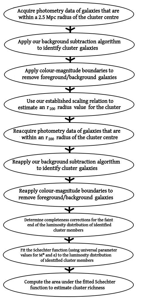
A brief outline of our multi-stage method to estimate the richness of a cluster can be seen in Figure 1. From which, the following subsections will describe our workflow in more detail.
2.1 Preparation of a photometric dataset to train a background subtraction model
To train our background subtraction model, we employed cluster galaxies that were identified by the Szabo et al. 2011 cluster catalogue (hereafter we refer to this cluster catalogue as the AMF11 catalogue) with an estimated photometric redshift between . We note that the AMF11 catalogue applied matched filters11 1 The matched filters were constructed from modeling positional, brightness and redshift information of cluster and field galaxy distributions. to galaxies observed in the Sloan Digital Sky Survey Data Release 6 (SDSS-II DR6, Adelman-McCarthy et al. 2008), where clusters were detected from maximising the likelihood of the matched filters whilst cluster galaxy membership identification was based on the proximity of the galaxy from the cluster center within 22 2 We refer to as the radius containing a mean density that is two hundred times greater than the critical density of the Universe. as well as whether the likelihood difference (i.e. the difference in likelihood of detecting a cluster with and without the presence of the galaxy) was above a specified threshold. The reason we decided to use the cluster galaxies from the AMF11 catalogue was because they assessed the cluster membership status of each galaxy based on their contribution to a combination of various cluster profiles (i.e. radial surface density, luminosity and redshift). In addition, their selection method does not discriminate between ‘blue’ and ‘red’ cluster galaxies, which means it is representative of different galaxy types in clusters.
We cross-matched these cluster galaxies with galaxies observed in the Sloan Digital Sky Survey Data Release 16 (SDSS-IV DR16, Ahumada et al. 2020) to obtain the following fifteen features that are based on SDSS-IV DR16 photometry33 3 We employed full-sky dust reddening maps (Schlegel et al. 1998; Schlafly & Finkbeiner 2011) to account for galactic extinction.: , , , , , , , , , , , , , and . For a cluster galaxy to be successfully cross-matched, the input astronomical coordinates must be within arcsecond from the astronomical coordinates of a galaxy within SDSS-IV DR16 as well as satisfying additional observing flags. These flags are as follows: the observed object should be a ‘primary’ observation44 4 We note that SDSS uses the term ‘primary’ to refer to the best imaging observation recorded for a survey object if it was seen multiple times during an observing run in an SDSS plate, whilst other observations of the object are known as ‘secondary’. and must be classified as a galaxy object type by the SDSS photometric pipeline. We also ensured that our cluster galaxy sample only contained galaxies with a unique SDSS object identifier to prevent accidentally including galaxies that may have been selected multiple times within our search radius due to very small angular separation between overlapping line-of-sight galaxies and errors in the astrometry. In addition, we did not include cluster galaxies that were within arcseconds (i.e. Mpc at ) of a subsample (see §§2.3 for further details) of cross-matched55 5 This involved identifying clusters that were within arcseconds (i.e. kpc at ) of each other in astronomical coordinate space and within (see Wen et al. 2009 for further explanation) of each other in redshift space. In addition, the clusters had to be observed within SDSS-IV DR16 between a redshift range of . clusters from the Wen & Han 2015 cluster catalogue (hereafter we refer to clusters from this catalogue as WH15 clusters) and Rykoff et al. 2014 cluster catalogue (hereafter we refer to clusters from this catalogue as redMaPPer clusters). This ensured that these clusters remained unseen for later usage in §§2.3. Furthermore, we applied a cut within colour-magnitude space (i.e. if greater than the percentile in and ) to remove any cluster galaxies that still appeared to have spurious photometry. It should be noted that throughout this work, we used and to visualise cluster and field galaxies in colour-magnitude diagrams due to straddling the break of cluster galaxies in our working redshift range.
Correspondingly, we also required a field galaxy66 6 We refer to interloping galaxies along a clusters line-of-sight as field galaxies. sample to train our background subtraction model to differentiate between cluster and field galaxies. However, we were unable to find a sizable catalogue containing identified field galaxies. This meant that we had to manually search for ‘field’ regions that did not visually appear to contain clusters from the full WH15 and redMaPPer cluster catalogues. This resulted in the identification of forty different ‘field’ regions, where the resultant astronomical sky map displaying the position of clusters and our proposed ‘field’ regions can be seen in Figure S1 (available online). We sampled galaxies from SDSS-IV DR16 that were within these ‘field’ regions. This involved applying a arcseconds (i.e. Mpc at ) search radius on each of the ‘field’ regions as well as reusing the same observing flags mentioned earlier within this section to obtain our field galaxy sample. The astronomical coordinates and number of observed field galaxies for each ‘field’ region are provided in Table 1. We did not include field galaxies that were within arcseconds from the cluster galaxies in the AMF11 catalogue to remove cluster galaxies that may have accidentally been included as part of the field regions. We also did not include field galaxies that were within arcseconds (i.e. Mpc at ) of the same subsample of cross-matched WH15 and redMaPPer clusters mentioned earlier within this section to ensure that the clusters remained unseen for later usage in §§2.3. Furthermore, we removed any field galaxies that were not within the same region of colour-magnitude space as our cluster galaxy sample, based on the observed minimum and maximum values for the cluster galaxies in and . This was intended to encourage our background subtraction model to learn to be more proficient at classifying galaxies with similar photometric properties. Subsequently, this yielded a total of field galaxies that had the same fifteen photometry features as our cluster galaxy sample. For this paper, we assumed that these field galaxies can be considered as ‘actual’ field galaxies.
| Right ascension | Declination | Number of observed galaxies |
|---|---|---|
| (degrees) | (degrees) | |
| 5.10408 | 21.0611 | 4488 |
| 5.77875 | 2.30955 | 7049 |
| 9.14699 | 33.7121 | 4030 |
| 10.4395 | -3.84934 | 5377 |
| 21.3533 | -3.02485 | 5595 |
| 23.0452 | 30.3202 | 5664 |
| 26.0012 | 23.8818 | 5024 |
| 28.3683 | 20.8955 | 2748 |
| 29.8579 | 11.0895 | 5108 |
| 38.6421 | -8.10943 | 5168 |
| 113.919 | 28.0332 | 5223 |
| 115.323 | 15.458 | 6310 |
| 121.916 | 0.109439 | 5518 |
| 129.971 | 51.2851 | 4753 |
| 143.518 | 63.0839 | 4564 |
| 144.097 | 47.3992 | 4929 |
| 158.633 | 56.6154 | 5982 |
| 166.196 | 20.0867 | 5861 |
| 177.951 | 65.8863 | 5733 |
| 196.86 | 15.2355 | 5885 |
| 207.127 | 65.0462 | 5711 |
| 214.632 | 3.77235 | 6109 |
| 219.239 | 62.0499 | 6009 |
| 226.958 | 54.9023 | 5346 |
| 231.26 | -0.0179 | 6696 |
| 235.973 | 18.662 | 7669 |
| 236.823 | 39.221 | 6421 |
| 238.422 | 58.5216 | 6760 |
| 255.233 | 18.8401 | 6079 |
| 263.834 | 28.0521 | 3565 |
| 316.524 | -6.36219 | 6273 |
| 316.54 | -1.56952 | 5201 |
| 326.258 | -6.56724 | 6597 |
| 332.263 | 28.8328 | 4580 |
| 332.498 | 19.5978 | 4043 |
| 333.873 | 24.14 | 4214 |
| 340.098 | 4.71022 | 4252 |
| 353.561 | 33.6502 | 4239 |
| 357.0789 | -4.69765 | 5103 |
| 359.369 | 17.4744 | 5809 |
We decided to set the redshift values of galaxies in our cluster and field galaxy samples to be based only on the photometric redshifts estimated by SDSS-IV DR16. This would enable a more straightforward comparison between the redshift distributions of both samples if they were measured via the same approach. We note that SDSS-IV DR16 applied the kd-tree nearest neighbor fit algorithm (see Csabai et al. 2007 for further details) to estimate the photometric redshifts of individual galaxies. We also used their estimated photometric redshifts to further constrain galaxies within our cluster galaxy sample to only be between a redshift range of , whereas galaxies within our field galaxy sample were not redshift restricted to mimic field galaxies appearing along the line-of-sight of clusters. Although, we note that galaxies were not required to have photometric redshifts available to be included in our field galaxy sample. In addition, we computed the filter absolute magnitudes for the cluster and field galaxies based on their photometric redshifts and corresponding K corrections77 7 In order to estimate the amount of K correction required, we performed linear interpolation between redshift and filter K corrected values determined from a simple stellar population model (see Bruzual & Charlot 2003 for further details)..
We note that our background subtraction model will learn to identify all cluster galaxies between a redshift range of , which may result in overcounting of cluster galaxies within a cluster if there are other clusters along the line-of-sight. To limit this effect, we decided to establish colour-magnitude boundaries within colour-magnitude space when applying our background subtraction model. These boundaries are designed to capture the majority of the population of cluster galaxies at specific redshifts. We first computed the median values of and for cluster galaxies in our cluster galaxy sample across redshift intervals of that are centered in redshift bins from to with step sizes of , as shown in Figure 2. We then manually determined appropriate lower and upper boundaries of and for each redshift bin. This would result in ‘L-shaped’ boundaries around the cluster galaxies at a given redshift, where an example of the ‘L-shaped’ boundaries for cluster galaxies at is shown in Figure 3. We then applied these colour-magnitude boundaries to our cluster galaxy sample across redshift bin sizes of to remove any cluster galaxies that were not within the colour-magnitude boundaries at their respective redshift. Subsequently, this yielded a total of cluster galaxies that were available to train our background subtraction model. For this paper, we assumed that these cluster galaxies can be considered as ‘actual’ cluster galaxies.


In Figure S2 (available online), it can be seen that our cluster and field galaxies were taken from different areas across SDSS-IV DR16. This meant that our cluster and field galaxy samples were likely to be representative of the whole population of cluster (between a redshift range of ) and field galaxies. Moreover, in Figures 4, S3 and S4 (available online), it can be seen that our field galaxy sample had an overall noticeable disparity to our cluster galaxy sample within colour-magnitude space. This somewhat validated our approach for obtaining the field galaxies given the underlying differences in photometry between the majority of the cluster and field galaxies. Although, we also observed some overlap of the ‘blue’ and faint cluster galaxies with bright field galaxies. We expect that it may be more difficult for our background subtraction model to differentiate between the galaxy classes within these overlap regions of colour-magnitude space. Furthermore, in Figure 5 we display the photometric redshift, filter apparent magnitude and filter absolute magnitude distributions of galaxies in our cluster and field galaxy samples. It can be seen that we had fewer cluster and field galaxies at lower redshifts when compared to those at higher redshifts. This indicated that we would need to sample equally across different redshifts to prevent our background subtraction model from being biased towards any particular redshift. We note that the number of field galaxies decreased significantly after due to the observing limitations of SDSS-IV DR16 at higher redshifts, where SDSS-IV DR16 had a filter limiting magnitude of . We also noticed that there was a gradual drop in the number of cluster and field galaxies towards fainter magnitudes due to the incompleteness of cluster galaxies in the AMF11 catalogue and observing limitations of SDSS-IV DR16 respectively.


Finally, we partitioned our cluster and field galaxy samples into three different subsets, known as the training, validation and test sets. In particular, the training set would be used to train our background subtraction model, the validation set would be used to tune its hyper-parameters and the test set would be used to obtain an unbiased estimate of the predictive performance of our background subtraction model. This involved randomly selecting , and cluster galaxies within fixed redshift bin sizes of across a redshift range of to be within our training, validation and test sets, which resulted in a total of , and cluster galaxies respectively. We also randomly selected , and field galaxies to be within our training, validation and test sets respectively. It should be noted that we applied sampling weights88 8 The amount of sampling weightage applied to each field galaxy in our training and validation sets was based on the resultant likelihood of the filter apparent magnitude for the field galaxy under a normal distribution that was constructed from the mean and standard deviation of the filter apparent magnitudes of cluster galaxies in our training and validation sets. We also shifted the computed means by in our training and validation sets to ensure that the cluster and field galaxy distributions overlapped at all filter apparent magnitudes. In addition, we note that sampling with replacement was used when selecting field galaxies to be within our training and validation sets. when selecting field galaxies to be within our training and validation sets to ensure that the filter apparent magnitudes of the field galaxies overlapped with the filter apparent magnitudes of the cluster galaxies. This would expose our background subtraction model to a larger proportion of the more difficult instances (i.e. cluster and field galaxies that had very similar photometry) during its training. Furthermore, we wanted our training, validation and test sets to remain as realistic as possible. As such, we permitted the number of field galaxies to outnumber (i.e. we assumed that having three field galaxies for every cluster galaxy was appropriate) the number of cluster galaxies with these sets. Although, we only permitted random sampling (i.e. equal sampling weightage) of field galaxies in our test set. These properties can be seen in Figure 6.


2.2 Using a multi-stage machine learning algorithm to perform background subtraction
We employed an unsupervised deep learning algorithm, known as an autoencoder (AE, Rumelhart et al. 1985), as the first stage of our background subtraction model. Our overall objective for using an AE is to train it to learn to accurately reconstruct input data. The mechanism behind the AE can be separated into three main stages, that are known as the encoder network, bottleneck and decoder network. The overall architecture for a typical AE is shown in Figure 7.
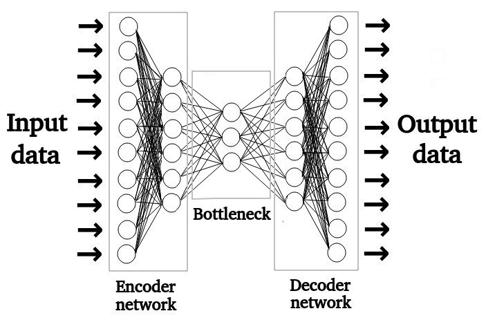
The encoder network is composed of fully-connected layers that are responsible for processing an input dataset by performing nonlinear transformations of the input data into a compressed representation. This is achieved by decreasing the number of nodes in the fully-connected layers as the size of the encoder network increases. The compression is maximised within the bottleneck, where the number of nodes in the bottleneck determines the amount of compression. The underlying objective of the bottleneck is to obtain the lowest dimensional representation of the data that captures the most generalisable aspects about the data. From which, the compressed data is then passed to the decoder network for reconstruction. This involves decompressing the compressed data back into its original input dimensionality by increasing the number of nodes in the fully-connected layers as the size of the decoder network increases. If the AE is properly trained, the reconstructed feature values should closely resemble the feature values of the input data. Overall, an AE can be considered as a type of dimensionality reduction-based algorithm since it focuses on reducing the dimensionality of the input data. However, we reconfigure its functionality from a dimensionality reduction-based algorithm into an outlier detection algorithm by also examining the differences between the reconstructed outputs and the input data. We note that the decoder network has the same but reversed architecture to the encoder network, where the number of nodes in the fully-connected layers increases rather than decreases as the size increases.
In order to train the AE to generate accurate reconstructions, we used the mean squared error as our loss function. This measured the similarity between all of the input and reconstructed feature values of galaxies via the following equation:
| (1) |
where is the number of input features, is the input feature values and is the reconstructed feature values.
We set the batch size, learning rate, optimiser algorithm99 9 We recommend the reader to refer to Ruder 2016 for an overview of different optimiser algorithms. and architecture layout1010 10 We considered the number of nodes in the bottleneck to be the most significant component of an AE’s architecture since it is influential in the amount of generalization learned. We decided that the number of nodes in the bottleneck should be a tunable hyper-parameter whilst the number of nodes for the hidden layers in the encoder and decoder networks would remain fixed. to be tunable hyper-parameters, where the full hyper-parameter search space is shown in Table 2.
| Tunable hyper-parameter name | Hyper-parameter search space |
|---|---|
| Batch size | 256 or 512 or 1024 or 2048 |
| Learning rate | 0.0001 or 0.001 or 0.01 or 0.1 |
| Optimiser algorithm | Adaptive Moment Estimation (Adam) or Adaptive Delta (Adadelta) or Adaptive Gradient Optimiser (Adagrad) or Adam Based On The Infinity Norm (Adamax) or Adam With Nesterov Momentum (Nadam) or Stochastic Gradient Descent (SGD) or Root Mean Squared Propagation (RMSprop) |
| Architecture layout (number of nodes and hidden layers in the encoder network and bottleneck) | 1 (13 nodes in first hidden layer, 11 nodes in second hidden layer, 9 nodes in third hidden layer, 7 nodes in the fourth hidden layer and 1 node in the bottleneck) or 2 (13 nodes in first hidden layer, 11 nodes in second hidden layer, 9 nodes in third hidden layer, 7 nodes in the fourth hidden layer and 3 nodes in the bottleneck) or 3 (13 nodes in first hidden layer, 11 nodes in second hidden layer, 9 nodes in third hidden layer, 7 nodes in the fourth hidden layer and 5 nodes in the bottleneck) |
We employed a separate machine learning algorithm, known as logistic regression (see Morgan & Teachman 1988 for further details), as the second stage of our background subtraction model. This served to convert the outputs of the AE into class predictions. In particular, we used the known class labels as the target variable and the mean squared error between the input and reconstructed feature values as the input variable, where if an input was poorly reconstructed by the AE then the corresponding mean squared error will be large too. From which, the logistic regression algorithm determines whether a galaxy should be classified as a cluster or field galaxy (i.e. the galaxy class with the higher predicted probability) when given the mean squared error of each galaxy. In this work, we decided to use the defaulted hyper-parameter values for the logistic regression algorithm (N.B. without regularisation) in the Scikit-Learn (Pedregosa et al. 2011) machine learning library since we primarily wanted to examine the influence of the AE in our background subtraction model. We expect that tuning the hyper-parameters for the logistic regression algorithm may slightly improve the overall predictive performance of our background subtraction model but this can be explored further in future work. It should be noted that the logistic regression algorithm minimised the following loss function during its training:
| (2) |
where is the number of inputs, is the true class value (i.e. either or ) and is the predicted probability (i.e. between and ) of being a galaxy class. This loss function measured the difference between predicted probability and true class value of galaxies.
We utilised a random search (see Bergstra & Bengio 2012 for further details) strategy to examine the predictive performance of our background subtraction model with different hyper-parameter combinations, where random search is a computationally efficient approach that does not need to examine every hyper-parameter combination. Instead, it considers that hyper-parameter optimization can be characterised by a Gaussian process, such that only a minority of hyper-parameter combinations are actually important. For example, we can assume that a randomly selected hyper-parameter combination has a ninety-five per cent probability of being situated within the top five per cent of all possible hyper-parameter combinations from the optimum after conducting only sixty iterations of random search. At the same time, we employed a Monte Carlo cross-validation (see Morgan & Teachman 1988 for further details) strategy to examine the variability of the predictive performance of our background subtraction model with different weight initialisations and dataset compositions. This involved repeated random sampling of new training, validation and test sets over ten iterations to measure the average predictive performance across the ten iterations. Ideally, we aimed to select a hyper-parameter combination that offered consistency and good predictive performance.
To determine the optimal hyper-parameter combination of our background subtraction model, we utilised the trapezium rule to compute the area under a precision-recall curve (AUCPR, Boyd et al. 2013) for each hyper-parameter combination, which is based on the following set of equations:
| (3) |
| (4) |
| (5) |
where TP is the number of correctly classified ‘actual’ cluster galaxies, FP is the number of incorrectly classified ‘actual’ cluster galaxies and FN is the number of incorrectly classified ‘actual’ field galaxies. Briefly, this metric measured the proportion of predictions that were predicted as cluster galaxies as well as the proportion of ‘actual’ cluster galaxies that were recovered across all class probability thresholds. It is ideal for assessing the predictive performance of a model that focuses on correctly identifying ‘rare’ instances (i.e. when there is a class imbalance). The optimal hyper-parameter combination would maximise the AUCPR for galaxies in our validation set.
Next, we determined the corresponding optimal class probability threshold when using the optimal hyper-parameter combination. This involved comparing the F1 score (Lipton et al. 2014) yielded for each class probability threshold (i.e. from to with class probability threshold step sizes of ) via the following equation:
| (6) |
This metric was similar to AUCPR in functionality except it only considered the predictive performance at a specific class probability threshold. The optimal class probability threshold would maximise the F1 score for galaxies in our validation set.
Lastly, we determined the overall classification accuracy of our background subtraction model at distinguishing between cluster and field galaxies in our test set. This involved computing the balanced accuracy (Brodersen et al. 2010) when using the optimal class probability threshold and optimal hyper-parameter combination via the following equation:
| (7) |
where TP is the number of correctly classified ‘actual’ cluster galaxies, TN is the number of correctly classified ‘actual’ field galaxies, FP is the number of incorrectly classified ‘actual’ cluster galaxies and FN is the number of incorrectly classified ‘actual’ field galaxies. The primary advantage of using balanced accuracy rather than conventional classification accuracy is that balanced accuracy takes into account class imbalance whereas conventional classification accuracy assumes equal class sizes when measuring the predictive performance of a binary classification model.
2.3 Establishing a scaling relation to estimate
It is beneficial to measure the richness of clusters within a characteristic radius (e.g. , , ) because it enables a more straightforward comparison of cluster richness across different cluster catalogues. We decided to establish a scaling relation that predicts values for the characteristic radius of cross-matched WH15 and redMaPPer clusters from §§2.1. We note that WH15 used a friend-of-friend grouping algorithm on galaxies with known spectroscopic or photometric redshifts to identify clusters in the Sloan Digital Sky Survey Data Release 12 (SDSS-III DR12, Alam et al. 2015) whilst redMaPPer used a red-sequence fitting algorithm on galaxies within colour-magnitude space to identify clusters in the Sloan Digital Sky Survey Data Release 8 (SDSS-III DR8, Aihara et al. 2011). Subsequently, we obtained a total of cross-matched WH15 and redMaPPer clusters between a redshift range of . We decided to use these clusters because they were found via two conventional approaches for cluster detection. This enabled us to directly compare the consistency of richness estimates from using our novel cluster galaxy identification technique versus other cluster galaxy identification techniques. In this proof-of-concept study, we choose to employ only a subsample of cross-matched WH15 and redMaPPer clusters when creating our scaling relation for time efficiency.
We also decided to use as our characteristic radius since the cluster galaxies in our training and test sets from the AMF11 catalogue were originally sampled within . In particular, we utilised values that were estimated by WH15 as the dependent variable in our scaling relation, where their estimates were computed via a scaling relation between measurements from X-ray/weak lensing observations and total luminosity in the band of all the identified cluster galaxies. For this work, we assumed that these values can be considered as ‘actual’ values. In Figure S5 (available online), we noticed that there was a strong linear relationship between WH151111 11 We refer to the variable from the WH15 catalogue as WH15 richness, where they computed cluster richness by measuring the total luminosity of identified galaxy members as a function of the typical luminosity of galaxies in the filter. and redMapper richness1212 12 We refer to the variable from the redMaPPer catalogue as redMaPPer richness, where they computed cluster richness by determining an expected richness which would yield the observed projected density, filter magnitudes and multiple colour indices of the identified red-sequence galaxies.. This means that we can directly compare our predicted richnesses with the richness estimates of redMaPPer. Furthermore, we noticed that there was a non-linear relationship between and both WH15 and redMaPPer richnesses which was in accordance with the empirical richness-size relation observed in Hansen et al. 2005, where our ‘actual’ values appeared to have greater variability at lower richnesses. As such, we expected that our scaling relation would have greater variability in at lower richnesses too.
We then partitioned the cross-matched WH15 and redMaPPer clusters into a training set and test set. We nominally referred to these sets as the CMWR (i.e. cross-matched WH15 and redMaPPer) training and test sets to avoid confusion with the training and test sets created in §§2.1. The purpose of having the CMWR training set was to determine the best fit coefficients of our scaling relation whilst the purpose of having the CMWR test set was to measure the predictive performance of our learned scaling relation. Since we knew the spectroscopic redshift of the CMWR clusters, we segmented them into fixed redshift bin sizes of . This ensured that our training and test sets contained clusters from across the redshift scale via stratified sampling1313 13 Stratified sampling is a strategy that minimises selection bias by splitting a dataset into new distributions that approximately resemble the original distribution.. This involved randomly allocating approximately half of the clusters within each redshift bin into both sets, which resulted in our CMWR training and test sets containing clusters each. The spectroscopic redshift and richness distributions of clusters in our CMWR training and test sets can be seen in Figure 8.


Next, we applied a search radius of Mpc at each cluster’s spectroscopic redshift as well as reapplying the same observing flags mentioned in §§2.1 to acquire galaxies from SDSS-IV DR16. This gave us a total of galaxies, where our CMWR training set consisted of galaxies and our CMWR test set consisted of galaxies. We then applied our background subtraction model and colour-magnitude boundaries to count the number of cluster galaxies within each cluster. We established a linear scaling relation that was based on the number of identified cluster galaxies as an independent variable and as the dependent variable. This involved learning the best fit coefficients by minimising the residual sum of squares between the dependent and independent variables in a linear regression algorithm from the Scikit-Learn machine learning library, where we again used the defaulted hyper-parameter values for the linear regression algorithm. We note that our cross-matched WH15 and redMaPPer cluster sample contained many clusters with low richness but only a few clusters with high richness. As such, we decided to assign the WH15 richness of each cluster as individual weights in the linear regression algorithm to minimise the effect of overfitting to potential outliers from clusters with low richness.
2.4 Preparation of a photometric dataset to estimate individual cluster richnesses
In order to measure richness within of individual clusters, we first approximated for clusters in our CMWR training and test sets using the learned scaling relation from §§2.3 to reacquire galaxies within from SDSS-IV DR16. We nominally referred to these new sets as the CMWR- training and test sets to avoid confusion with the CMWR training and test sets created in §§2.3. Similar to before, the purpose of having the CMWR- training set was to determine the best fit coefficients of a luminosity distribution fitting function whilst the purpose of having the CMWR- test set was to measure the predictive performance of the learned luminosity distribution fitting function. We obtained a total of galaxies in our CMWR- training set and galaxies in our CMWR- test set. The resultant color-magnitude diagrams of galaxies in our CMWR- training and test sets is shown in Figure 9.


2.5 Using a luminosity distribution fitting function to estimate individual cluster richnesses within
We adopted a similar approach to the methodology described in Schechter 1976 to estimate the richness of individual clusters. Schechter 1976 showed that it was possible to use a luminosity distribution fitting function (i.e. the Schechter function) to do this. Briefly, this involved fitting the function to a composite luminosity distribution of cluster galaxies in order to determine best fit parameter values of the function. Then Schechter 1976 assumed that the best fit parameter values for and can be applied universally to the luminosity distribution of individual clusters to locally fit for and thus estimate cluster richness. The Schechter function is expressed via the following equation:
| (8) |
where is absolute magnitude, is the number of galaxies per unit magnitude, is the ‘characteristic’ magnitude at which the distributions of faint and bright galaxies rapidly changes and is the faint end slope parameter that describes the distribution of galaxies fainter than . We note that and directly influence the steepness of the bright and faint ends in the Schechter function whilst varies based on the observed number of galaxies within magnitude bins.
Firstly, we applied our background subtraction model and colour-magnitude boundaries to identify cluster galaxies from the CMWR- training set. We then performed Chi-squared fitting1414 14 We used the curve fit function from the SciPy Python library (Virtanen et al. 2020) to perform Chi-squared fitting of the Schechter function, which returned the best fit parameter values that minimised the Chi-squared fitting error and also returned an estimated covariance matrix of the best fit parameter values. with initialisation bounds for (i.e. between and ), (i.e. between and positive infinity) and (i.e. between and ) when fitting the Schechter function to a composite luminosity distribution that consisted of a subsample of identified cluster galaxies which appeared to have high completeness (i.e. greater than per cent when using a base-10 logarithmic scale for the counts) between a restricted filter absolute magnitude (i.e. between and ) and redshift (i.e. between and ) range. At the same time, we also explored various filter absolute magnitude bin sizes (i.e. from to with step sizes of ) to obtain an optimal filter absolute magnitude bin size that minimised the Chi-squared fitting error and yielded galaxies across five or more filter absolute magnitude bins. Furthermore, we approximated the uncertainty in the number of identified cluster galaxies within each magnitude bin by assuming that the uncertainty followed a Poisson sampling hypothesis1515 15 A Poisson sampling hypothesis assumed that the distribution of galaxies is dictated by a Poisson process, such that the standard deviation of the counts within each magnitude bin was based on the square root of the count (Schechter 1976). when fitting the Schechter function. From which, we determined an optimal absolute magnitude bin size and best fit parameter values for , and , where we also assumed that the best fit parameter values for and can be applied universally to the luminosity distribution of individual clusters.
We remind the reader that our background subtraction model had not yet been corrected for the incompleteness of faint galaxies from observing limitations. This meant that we had to derive completeness corrections for the luminosity distribution (i.e. using filter absolute magnitudes) of individual clusters at different redshifts. Initially, we grouped the identified cluster galaxies from the CMWR- training set into redshift intervals of that were centered in redshift bins from to with step sizes of , where identified cluster galaxies from different redshifts can go into multiple bins. Next, we fitted a per cent completeness line across adjacent filter apparent magnitude bins1616 16 We used an filter apparent magnitude bin size that corresponded to the optimal filter absolute magnitude bin size. In addition, when working with the luminosity distribution of individual clusters we only considered cluster galaxies within an filter absolute magnitude range of to , where was the filter absolute magnitude limit that was used to determine WH15 richness in Wen & Han 2015. that were on the bright side of the peak and within the completeness limit of the AMF11 catalogue for each redshift interval. We then approximated the completeness fraction of the faintest filter apparent magnitude bin (N.B. we considered the two faintest magnitude bins on the bright side of the peak beyond and three faintest magnitude bins on the bright side of the peak beyond as the incompleteness of galaxies became more visibly noticeable for more magnitude bins at higher redshifts) by calculating the fraction in the expected number of cluster galaxies (i.e. based on the per cent completeness line) to the observed number of cluster galaxies (i.e. identified by our background subtraction model).
We applied these completeness fractions to the luminosity distribution of individual clusters by multiplying the observed count of the faintest (N.B. we again considered the two faintest magnitude bins on the bright side of the peak beyond and three faintest magnitude bins on the bright side of the peak beyond ) filter absolute magnitude bin1717 17 Since our completeness fractions were measured in filter apparent magnitudes, we had to convert between filter apparent magnitudes and filter absolute magnitudes to determine the relevant completeness fraction. on the bright side of the peak by the completeness fraction of the corresponding filter apparent magnitude bin within the nearest redshift interval. We then replaced the uncertainty range of the observed count in the magnitude bin with this computed completeness correction value as the new lower and upper uncertainty limits when performing Chi-square fitting. This ensured that the Schechter function did not fit to incomplete filter absolute magnitude bins.
Finally, we estimated cluster richnesses within by integrating1818 18 We utilised the incomplete Gamma function (see Equation in Schechter 1976) to compute the integral. the locally fit Schechter function. This gave us the expected number of cluster galaxies within that had an filter absolute magnitude brighter than . We also compared our estimated cluster richnesses with WH15 richnesses, spectroscopic redshift, ‘actual’ and redMaPPer richnesses in order to examine the predictive performance of the optimal filter absolute magnitude bin size and best fit parameters for and in the Schechter function. We note that WH15 richness was specific to whereas redMaPPer richness was specific to redMaPPer’s own scaling radius rather than . This meant that we could directly quantify the error between our estimated cluster richnesses and WH15 richnessses by using root mean squared error as a metric.
3 Results
3.1 Model tuning analyses
3.1.1 Analysis of our trained background subtraction model
We conducted ten iterations of Monte Carlo cross-validation to measure the variability of the predictive performance of our background subtraction model, as well as conducting sixty iterations of random search on the tunable hyper-parameters of our background subtraction model, to determine an optimal hyper-parameter combination that maximised the AUCPR of galaxies in our validation set. It can be seen in Table S1 (available online) that the optimum hyper-parameter combination was as follows: optimal batch size = ; optimal learning rate = ; optimal optimiser algorithm = RMSprop and optimal architecture layout = . This optimum hyper-parameter combination yielded a mean AUCPR value of per cent with a standard deviation of per cent for galaxies in our validation set. Furthermore, it can be seen in Table S2 (available online) that the optimum class probability threshold was , when using the optimum hyper-parameter combination. This optimum class probability threshold yielded a F1 score of per cent for galaxies in our validation set.
3.1.2 Analysis of our established scaling relation to estimate
We constructed a scaling relation using clusters in our CMWR training set to estimate the of each cluster when given the number of cluster galaxies identified by our background subtraction model as an input. The best fit coefficients of our scaling relation were determined by minimising the weighted residual sum of squares between the independent and dependent variables, where our scaling relation is defined via the following equation:
| (9) |
where is the predicted , is the number of cluster galaxies identified within a Mpc search radius at each cluster’s spectroscopic redshift and the uncertainty represents the standard error of the parameter estimates. In Figure 10, it can be seen that there was a larger drop in the number of cluster galaxies identified by our background subtraction model at higher redshifts (i.e. ) when compared to the number of identified cluster galaxies at lower redshifts with the same ‘actual’ values. This was likely due to cluster galaxies at higher redshifts having larger observed photometric errors, which made it more difficult for our background subtraction model to identify these cluster galaxies. We note that we obtained a Pearson correlation coefficient value of between the number of identified cluster galaxies and ‘actual’ variables. We also observed that both WH15 and redMaPPer richnesses appeared to somewhat linearly increase with ‘actual’ and the number of identified cluster galaxies. Furthermore, in Figure 11, we compared the predictive performance of our predicted with the ‘actual’ , where we found that our predicted was quite comparable to the ‘actual’ across all cluster sizes. Although, we noticed there was greater variability in the predicted at lower cluster richnesses, where we obtained a root mean squared error of and a median absolute percentage error of per cent between our predicted and ‘actual’ values.


3.1.3 Analysis of the best fit parameters for a luminosity distribution fitting function to estimate individual cluster richnesses Within
We used a Chi-squared fitting approach to determine the best fit parameters of the Schechter function when fitting to a composite luminosity distribution that consisted of a subsample of identified cluster galaxies from our CMWR training set with high completeness. We also simultaneously determined an optimal filter absolute magnitude bin size that minimised the Chi-squared fitting error and yielded galaxies across five or more filter absolute magnitude bins. In Table S3 (available online), we identified an optimal filter absolute magnitude bin size of that had corresponding best fit parameter values of = with a standard deviation of ; = with a standard deviation of and = with a standard deviation of . In Figure 12, we display the composite luminosity distribution and fitted Schechter function using the optimal filter absolute magnitude bin size and best fit parameter values.

We then used the optimal filter absolute magnitude bin size and best fit parameter values for and to fit the Schechter function to the luminosity distribution of individual clusters from our CMWR- training set. This enabled us to estimate individual cluster richnesses by integrating the locally fit Schechter function. Subsequently, we obtained a root mean squared error of and a median absolute percentage error of per cent between our estimated cluster richnesses and WH15 richnesses within . In Figure 13, we noticed that WH15 richnesses had a strong linear correlation with our estimated cluster richnesses. We also observed that spectroscopic redshifts seemed to have no distinguishable correlation with our estimated cluster richnesses. In addition, we noticed that there was a strong linear correlation between ‘actual’ , redMaPPer richnesses and our estimated cluster richnesses. These results confirmed that our approach to estimate individual cluster richnesses was appropriate since we did not train any of our models to minimise cluster richness prediction error but we still obtained strong correlations with WH15 and redMaPPer richnesses. Furthermore, we were aware that our CMWR- training set contained clusters that were not truly unseen, as we had utilised these clusters before to create our scaling relation. Although, it was still interesting to test our methodology on clusters that were seen and unseen to compare differences in predictive performance.

3.2 Overall performance analyses with test sets
We further assessed our entire methodology on clusters belonging to our various test sets to obtain an unbiased evaluation of the true predictive performance of our models. Firstly, we applied our background subtraction model to cluster and field galaxies in our test set. This yielded a F1 score of per cent and a balanced accuracy of per cent when using the optimal hyper-parameter combination and optimal class probability threshold for our background subtraction model. In Figure 14, we display a direct comparison of the ‘actual’ and predicted cluster and field galaxies. It can be seen that our background subtraction model learned to correctly classify almost all of the field galaxies surrounding the cluster galaxies but it made more incorrect classifications in regions where the ‘actual’ cluster and field galaxies had greater overlap within colour-magnitude space. Meanwhile, in Figure 15, we compared the number of cluster and field galaxies identified by our subtraction model across redshift bin sizes of . At lower redshifts (i.e. ), we noticed that our background subtraction model slightly underestimated (i.e. misclassified ‘actual’ field galaxies as cluster galaxies or misclassified ‘actual’ cluster galaxies as field galaxies) the overall number of ‘actual’ cluster and field galaxies. In particular, we noticed a larger drop in the number of identified ‘actual’ cluster galaxies between , which was similar to our observation in Figure 10. Correspondingly, at higher redshifts (i.e. ), we found that our background subtraction model correctly classified almost all of the galaxies. In Figures 16 and 17, we compared the number of cluster and field galaxies identified by our subtraction model across filter apparent and absolute magnitude bin sizes of respectively. In both magnitude distributions, we noticed that our background subtraction model slightly underestimated the overall number of ‘actual’ cluster galaxies at all magnitudes. We also noticed that our background subtraction model slightly underestimated the overall number of ‘actual’ field galaxies at intermediate brightnesses (i.e. between and in filter apparent magnitude and between and in filter absolute magnitude) but correctly classified almost all of the other fainter and brighter ‘actual’ field galaxies. Furthermore, in Figure 18 we examined the proportion of ‘red’ and ‘blue’ ‘actual’ cluster galaxies that were identified by our background subtraction model at different redshifts. We found that our background subtraction model identified per cent of ‘red’ ‘actual’ cluster galaxies and recovered per cent of ‘blue’ ‘actual’ cluster galaxies between a redshift range of . This indicated that our background subtraction model was more confident at identifying ‘red’ ‘actual’ cluster galaxies than ‘blue’ ‘actual’ cluster galaxies, which was likely due to the ‘blue’ ‘actual’ cluster galaxies having greater overlap with field galaxies within colour-magnitude space.


We then applied our learned scaling relation and colour-magnitude boundaries to clusters in our CMWR test set to approximate for each cluster. In Figure 19, we noticed that the number of identified cluster galaxies and ‘actual’ was relatively consistent with our learned scaling relation from Figure 10. From which, we obtained a Pearson correlation coefficient value of between the number of identified cluster galaxies and ‘actual’ variables in Figure 19. We also noticed that our predicted and ‘actual’ values in Figure 20 was similar to the overall trend observed in Figure 11, where we obtained a root mean squared error of and a median absolute percentage error of per cent between our predicted and ‘actual’ values in Figure 20.


Finally, we examined the predictive performance of the optimal filter absolute magnitude bin size and best fit parameter values for and in the Schechter function on individual clusters in our CMWR- test set. In Figure 21, we noticed that the overall trends between our estimated cluster richnesses and WH15 richnesses with spectroscopic redshifts, ‘actual’ and redMaPPer richnesses were again consistent with Figure 13, where our estimated cluster richnesses had no distinct correlation with spectroscopic redshifts and our estimated cluster richnesses linearly increased with ‘actual’ and redMaPPer richnesses. Subsequently, we obtained a root mean squared error of and a median absolute percentage error of per cent between our estimated cluster richnesses and WH15 richnesses within .

3.3 Examining the importance of input features to our background subtraction model
In Figure 22, we examined the importance of each input feature to our background subtraction model. This involved randomly shuffling the data of each input feature and then applying our background subtraction model on the dataset to observe how the shuffled feature impacted the predictive performance. This strategy is known as permutation feature importance testing (Breiman 2001), where the permutation scores were based on the number of ‘actual’ cluster galaxies identified by our background subtraction model. In particular, a lower permutation score for an input feature implied greater reliance of our background subtraction model on that specific input feature to provide good predictive performance, because randomly shuffling the data for an important input feature would result in fewer ‘actual’ cluster galaxies being identified. We applied this permutation feature importance test to galaxies in our test set, which originally contained cluster galaxies. Subsequently, we observed that , , , , , , and appeared to have greater significance to our background subtraction model whereas , , , , , and appeared to have lesser significance to our background subtraction model. Although, it is important to note that our background subtraction model had effectively utilised all the input features since the number of identified ‘actual’ cluster galaxies for each input feature was still only a fraction of the original number of ‘actual’ cluster galaxies.

4 Discussion
In Figure 5, we observed that the photometric redshift distribution of galaxies in our cluster galaxy sample was skewed towards higher redshifts, such that higher redshift cluster galaxies were overrepresented. To achieve a fair representation of cluster galaxies at different redshifts in our background subtraction model, we randomly sampled a fixed number of cluster galaxies within fixed redshift bin sizes of when creating our training, validation and test sets. This ensured that our background subtraction model was exposed to equal numbers of cluster galaxies at various redshifts within colour-magnitude space. We also exposed our background subtraction model to equal numbers of cluster and field galaxies during its training. This was to ensure a fair representation of the different galaxy classes in our background subtraction model.
We initially constrained our training sample to only spectroscopically confirmed cluster galaxies from the AMF11 catalogue but we quickly noticed that the training sample itself had a significant drop in the number of faint cluster galaxies across all redshifts when compared to the non-spectroscopically confirmed cluster galaxies. As such, we decided not to adopt this constraint when training our background subtraction model. Furthermore, we did not utilise spectroscopically confirmed field galaxies since it was difficult to acquire a sample that was representative of all potential foreground and background galaxies encountered within a random field. Although, in future work this may be possible since the number of spectroscopically confirmed cluster and field galaxies would naturally increase over time.
When constructing our scaling relation, we employed ‘actual’ values that were estimated from a scaling relation (see Equation in Wen et al. 2012) that was based on the total filter luminosity of identified cluster galaxies within a Mpc radius from the cluster center at each clusters redshift. This meant that the errors from their estimated values would have carried over into our estimated values too. In future work, we could instead consider employing values from X-ray cluster catalogues as X-ray emission measurements are not as significantly influenced by projection effects (Ebeling et al. 2010). This would improve the overall precision of our ‘actual’ values and thus improve the precision of our cluster richness estimates within . Furthermore, we can establish a scaling relation for any radii, not only , as long as we have sufficient data to enable the construction of a scaling relation for the radii.
In Figures 13 and 21 we did not observe any redshift biases in our estimated cluster richnesses after we applied completeness corrections to account for fewer observed galaxies at the faint end of the luminosity distribution of individual clusters. This indicated that incompleteness of our cluster galaxy sample from the AMF11 catalogue had a bigger impact on estimating cluster richnesses than incompleteness from misclassifications by our background subtraction model. Although, in Figures 10, 15 and 19 we observed a larger drop in the number of identified cluster galaxies at higher redshifts (i.e. ) when compared to the number of identified cluster galaxies at lower redshifts. We believed that this could be due to the cluster galaxies at higher redshifts having larger photometric errors than cluster galaxies at lower redshifts, which can be seen in Figure 18 by the increased scatter between data points as redshift increased. Naturally, this would make it more difficult for our background subtraction model to identify them. As such, we would expect there to be fewer cluster galaxies identified at higher redshifts, since we did not truly account for cluster galaxies having larger photometric errors at higher redshifts in our background subtraction model. In the future, it would be beneficial to obtain and utilise a larger cluster galaxy sample when training our background subtraction model, which would hopefully reduce this effect by exposing the model to more examples. It may also be beneficial to employ an algorithm that can learn to interpolate regions within colour-magnitude space in order to account for the larger photometric errors at higher redshifts, such as a variational autoencoder (Kingma & Welling 2013).
In this work, we used the Schechter function to fit to the luminosity distribution of identified cluster galaxies, where it was important to review the cluster membership status of each individual galaxy in order to minimise severe contamination from bright interloping field galaxies when fitting the Schechter function. Although, we were aware of alternative luminosity functions that could be used to fit to the luminosity distribution of cluster galaxies. Two other commonly used luminosity functions1919 19 We recommend the reader to refer to Sarazin 1986 for an overview of different luminosity functions. include the Zwicky function (Zwicky 1957) and Abell function (Abell 1975). Briefly, the Zwicky function is fitted by considering the difference in magnitude of each cluster galaxy from the brightest cluster galaxy whereas the Abell function is fitted by combining two separately fitted analytical functions. This means that the Zwicky function requires identifying the brightest cluster galaxy beforehand whereas the Abell function is not continuous at all luminosities. We decided to use the Schechter function over these other luminosity functions because the Schechter function did not have strict prerequisite conditions and offers continuity (i.e. it was composed of a power law and an exponential function) at all luminosities (Sarazin 1986).
We fitted the Schechter function to a composite luminosity distribution that consisted of a subsample of identified cluster galaxies with high completeness to obtain best fit parameter values of = with a standard deviation of ; = with a standard deviation of and = with a standard deviation of . We did not allow to be greater than or lesser than when performing Chi-squared fitting, as we assumed that it would be unphysical for the number of cluster galaxies to be decreasing or increasing rapidly at fainter magnitudes respectively. We also did not set any specific bounds for and , since these parameters were more dependent on the given data. We attempted to compare our best fit parameter values for and to the best fit parameter values of and found in the literature from cluster studies to determine whether our best fit parameter values for and were appropriate as ‘universal’ values. However, we found that the literature contained a wide range of values for and that depended on a variety of different factors (e.g. photometric system used, magnitude range examined, redshift range examined, cluster mass range examined, composition of galaxy types in cluster sample, background subtraction method used). Although, we noticed that some typical values obtained for and span approximately from to and to respectively (e.g. Oegerle et al. 1987; Oegerle & Hoessel 1989; Valotto et al. 1997; Rauzy et al. 1998; Paolillo et al. 2001; Popesso et al. 2005). This suggested that our assumptions for and were not unreasonable.
We remind the reader that our approach for estimating cluster richness was based only on the number of cluster galaxies identified by our background subtraction model within a defined magnitude range and given search area. This would be particularly beneficial for cosmological studies (Sarazin 1986), such as comparing simulated and observed halo mass functions (e.g. Castro et al. 2016; Yennapureddy & Melia 2019), since it would reduce the complexity of modeling an appropriate selection function to correct for biases from post-processing (e.g. incorrect star/galaxy classification, deblending/interpolation issues, misestimated photometric redshifts) or survey conditions (e.g. flux limitations, oversaturation by bright stars, different aperture sizes) (Melin et al. 2005). In addition, our background subtraction method provides robustness when estimating cluster richness along any line-of-sight environment since it assesses the cluster membership status of galaxies based only on their photometric measurements. This is not easily achievable when using simple statistical-based or colour-based background subtraction methods. Furthermore, our background subtraction method does not require us to make any assumptions about the properties of the cluster and field galaxies since these properties are self-learned by the AE algorithm. This means that our background subtraction method is not intrinsically biased towards selecting different galaxy types.
In future work, it would be interesting to examine the applicability of our background subtraction method on different usage cases. These include studying the properties and evolution of identified cluster galaxies or deciding spectroscopic follow-ups of potential galaxy members in clusters or measuring the observed radial density, luminosity and redshift profiles of clusters. We also aim to extend this current work by also establishing an empirical scaling relation between our richness estimates and cluster dark matter halo masses, that have been inferred via weak gravitational lensing, in order to construct an observed halo mass function for constraining cosmological parameters. In addition, we intend to integrate our background subtraction method with our own cluster finder model (Deep-CEE, Chan & Stott 2019) and photometric redshift estimator model (Z-Sequence, Chan & Stott 2021) to mask or remove interloping line-of-sight galaxies in image data or photometric catalogue data respectively to further minimise their model predictions errors.
We note that there are various other types of conventional machine learning algorithms2020 20 We recommend the reader to refer to https://pyod.readthedocs.io/en/latest/pyod.models.html for an extensive list of outlier detection algorithms (Zhao et al. 2019). available, aside from AE’s, which could be used for the task of performing background subtraction. These could include the K-nearest neighbours algorithm (Fix 1951), K-means algorithm (Macqueen 1967), isolation forest algorithm (Liu et al. 2008), support vector machine algorithm (Cortes & Vapnik 2009) and XGBoost algorithm (Chen & Guestrin 2016). The reason we chose to utilise an AE over other conventional machine learning algorithms was due to the fact that an AE is a deep neural network, which is capable of self-learning the importance of input features. On the other hand, most conventional machine learning algorithms require important features to be manually extracted in order to attain good predictive performance, which can be time-consuming and difficult to do when there are many complex features (Liang et al. 2017; Notley & Magdon-Ismail 2018; O’ Mahony et al. 2019; Liu et al. 2022).
When training our background subtraction model, we used a Monte Carlo cross-validation strategy to determine an optimal hyper-parameter combination that offered the best predictive performance possible across different weight initialisations by performing random subsampling of our training and validation sets. Although, this may have resulted in some galaxies not being utilised at all (i.e. if the galaxy was not randomly chosen to be in any of our training, validation or test sets), which is not maximising data efficiency. In future work, we could employ a k-fold cross-validation strategy (Bengio & Grandvalet 2004) for hyper-parameter tuning and model evaluation. This would improve data efficiency and model generalisation as our background subtraction model would be evenly examined across all available data during its training and testing phases.
We performed permutation feature importance testing to determine which input features were deemed as important by our background subtraction model when identifying ‘actual’ cluster galaxies. From which, we found that the following input features displayed high significance: , , , , , , and . This tells us that our background subtraction model had learned to utilise most of the available photometric information in high dimensional colour-magnitude space. This was more efficient than only utilising a two dimensional colour-magnitude diagram, which is typically used when attempting to detect cluster galaxies within colour-magnitude space (e.g. Yee et al. 1999; Gladders & Yee 2005; Stott et al. 2009; Valentinuzzi et al. 2011). We believe that these specific input features were important to our background subtraction model due to two main reasons. Firstly, in Figure 14 it can be seen that the majority of the cluster and field galaxy population can be distinguished via filter magnitudes within colour-magnitude space. This explained why our background subtraction model prioritised several filter magnitudes when performing background subtraction. Secondly, in Figure 14 it can also be seen that a minority of cluster galaxies overlapped with field galaxies within colour magnitude space. This explained why our background subtraction model also prioritised several colours in combination with the filter magnitudes to distinguish between these overlapping cluster and field galaxies. Based on these reasons, it is not unreasonable to assume that our background subtraction model can recognise the broad spectral features (e.g. break) and overall shape of the observed spectral energy distribution2121 21 We recommend the reader to refer to Kennicutt 1992 for further details on the observed spectral energy distribution of different galaxies. of cluster galaxies2222 22 Clusters typically have a majority population of elliptical and lenticular galaxies with a minority population of spiral galaxies (Dressler 1980). at different redshifts.
In future work, it would be interesting to examine the impact from including additional features such as galaxy sizes, morphology and surface brightness as inputs for our background subtraction model. However, we note that we cannot easily reapply our method to galaxy surveys that do not readily provide information for all our required input features. Furthermore, our background subtraction model is not provided with redshift information as an input feature when distinguishing between cluster and field galaxies. Instead, we wanted our background subtraction model to self-learn about the photometric properties of cluster galaxies belonging to different redshift intervals, which is similar to how photometric redshifts of individual galaxies are estimated by empirical algorithms.
5 Conclusion
We present a proof-of-concept study of AutoEnRichness, a hybrid empirical and analytical approach that uses a multi-stage machine learning algorithm and a conventional luminosity distribution fitting approach to perform background subtraction and estimate cluster richnesses respectively. We utilised photometric data from the SDSS-IV DR16 to train our background subtraction model, which learned to reconstruct the photometry of cluster galaxies in order to distinguish between cluster and field galaxies. We then examined the predictive performance of our background subtraction model at distinguishing between cluster and field galaxies in a test set, which resulted in a balanced accuracy of per cent. Subsequently, we constructed a scaling relation that estimated when given the number of cluster galaxies identified by our background subtraction model within a search radius of Mpc at each cluster’s spectroscopic redshift. We utilised this learned scaling relation to resample galaxies within an radius for each cluster. Next, we fitted the Schechter function to a composite luminosity distribution that consisted of a subsample of cluster galaxies identified by our background subtraction model within that had high completeness. We used a Chi-squared fitting approach to determine an optimal filter absolute magnitude bin size of and best fit parameter values of = with a standard deviation of ; = with a standard deviation of and = with a standard deviation of . We then used the optimal filter absolute magnitude bin size and best fit parameter values for and to fit the Schechter function to the luminosity distribution of individual clusters. We estimated cluster richnesses within by computing the integral of the locally fit Schechter function. Lastly, we applied the optimal filter absolute magnitude bin size and best fit parameter values for and to another test set of clusters to obtain a median absolute percentage error of per cent between our estimated cluster richnesses and WH15 richnesses within . We note that the only cluster prerequisites for AutoEnRichness were the astronomical coordinates of the approximate cluster location as well as an initial cluster redshift estimate for computing appropriate cluster radii. We intend for AutoEnRichness to be combined with the Deep-CEE (Chan & Stott 2019) and Z-Sequence (Chan & Stott 2021) algorithms to obtain the key measurements (i.e. position from cluster detection and distance from redshift estimation respectively) needed for conducting astrophysics and cosmology research. In future work, it would be beneficial to develop a data pipeline that integrates AutoEnRichness with these other methods into an end-to-end process in preparation for usage on upcoming large-scale galaxy surveys, such as the Legacy Survey of Space and Time (Ivezić et al. 2019) and (Laureijs et al. 2011; Euclid Collaboration et al. 2019).
Acknowledgements
We would like to thank the anonymous referee for their thorough feedback which has improved the clarity of our paper.
We gratefully acknowledge the support from the Science and Technologies Facilities Council studentship funding. We thank members of the XMM Cluster Survey for useful discussions. We would also like to thank the developers of Vizier (Ochsenbein et al. 2000), TOPCAT (Taylor 2020), James Schombert at the University of Oregon, Edward L. Wright at the University of California, Los Angeles (Wright 2006), Scikit-Learn (Pedregosa et al. 2011), SciPy (Virtanen et al. 2020) and TensorFlow (Abadi et al. 2015) for allowing the open distribution and free usage of their software for research.
Funding for the Sloan Digital Sky Survey IV has been provided by the Alfred P. Sloan Foundation, the U.S. Department of Energy Office of Science, and the Participating Institutions.
SDSS-IV acknowledges support and resources from the Center for High Performance Computing at the University of Utah. The SDSS website is www.sdss.org.
SDSS-IV is managed by the Astrophysical Research Consortium for the Participating Institutions of the SDSS Collaboration including the Brazilian Participation Group, the Carnegie Institution for Science, Carnegie Mellon University, Center for Astrophysics | Harvard & Smithsonian, the Chilean Participation Group, the French Participation Group, Instituto de Astrofísica de Canarias, The Johns Hopkins University, Kavli Institute for the Physics and Mathematics of the Universe (IPMU) / University of Tokyo, the Korean Participation Group, Lawrence Berkeley National Laboratory, Leibniz Institut für Astrophysik Potsdam (AIP), Max-Planck-Institut für Astronomie (MPIA Heidelberg), Max-Planck-Institut für Astrophysik (MPA Garching), Max-Planck-Institut für Extraterrestrische Physik (MPE), National Astronomical Observatories of China, New Mexico State University, New York University, University of Notre Dame, Observatário Nacional / MCTI, The Ohio State University, Pennsylvania State University, Shanghai Astronomical Observatory, United Kingdom Participation Group, Universidad Nacional Autónoma de México, University of Arizona, University of Colorado Boulder, University of Oxford, University of Portsmouth, University of Utah, University of Virginia, University of Washington, University of Wisconsin, Vanderbilt University, and Yale University.
Data Availability
The AMF11 catalogue (Szabo et al. 2011) of individual cluster galaxies is publicly available on Vizier via: http://vizier.u-strasbg.fr/viz-bin/VizieR-3?-source=J/ApJ/736/21/mg. The SDSS-IV DR16 (Ahumada et al. 2020) photometry data of individual galaxies is also publicly available on Vizier via: http://vizier.u-strasbg.fr/viz-bin/VizieR?-source=V/154. Furthermore, the WH15 (Wen & Han 2015) and redMaPPer v6.3 (Rykoff et al. 2014) cluster catalogues can be found publicly via: http://vizier.u-strasbg.fr/viz-bin/VizieR-3?-source=J/ApJ/807/178/table3 and http://risa.stanford.edu/redmapper/.
References
- Abadi et al. (2015) Abadi M., et al., 2015, TensorFlow: Large-Scale Machine Learning on Heterogeneous Systems, http://tensorflow.org/
- Abell (1958) Abell G. O., 1958, ApJS, 3, 211
- Abell (1975) Abell G. O., 1975, Stars and Stellar Systems IX: Galaxies and the Universe, p. 601
- Adelman-McCarthy et al. (2008) Adelman-McCarthy J. K., et al., 2008, ApJS, 175, 297
- Ahumada et al. (2020) Ahumada R., et al., 2020, ApJS, 249, 3
- Aihara et al. (2011) Aihara H., et al., 2011, ApJS, 193, 29
- Alam et al. (2015) Alam S., et al., 2015, ApJS, 219, 12
- Alpaslan et al. (2012) Alpaslan M., et al., 2012, MNRAS, 426, 2832
- Amodeo et al. (2016) Amodeo S., Ettori S., Capasso R., Sereno M., 2016, A&A, 590, A126
- Bahcall (1988) Bahcall N. A., 1988, ARA&A, 26, 631
- Balland & Blanchard (1995) Balland C., Blanchard A., 1995, arXiv e-prints, pp astro–ph/9510130
- Bengio & Grandvalet (2004) Bengio Y., Grandvalet Y., 2004, The Journal of Machine Learning Research, 5, 1089
- Bergstra & Bengio (2012) Bergstra J., Bengio Y., 2012, The Journal of Machine Learning Research, 13, 281
- Biviano & Girardi (2003) Biviano A., Girardi M., 2003, ApJ, 585, 205
- Boué et al. (2008) Boué G., Adami C., Durret F., Mamon G. A., Cayatte V., 2008, A&A, 479, 335
- Boyd et al. (2013) Boyd K., Eng K. H., Page C. D., 2013, in Proceedings of the 2013th European Conference on Machine Learning and Knowledge Discovery in Databases - Volume Part III. ECMLPKDD’13. Springer-Verlag, Berlin, Heidelberg, pp 451–466, doi:10.1007/978-3-642-40994-3_29, https://doi.org/10.1007/978-3-642-40994-3_29
- Breiman (2001) Breiman L., 2001, Machine Learning, 45, 5
- Brodersen et al. (2010) Brodersen K. H., Ong C. S., Stephan K. E., Buhmann J. M., 2010, in 2010 20th International Conference on Pattern Recognition. pp 3121–3124, doi:10.1109/ICPR.2010.764
- Bruzual & Charlot (2003) Bruzual G., Charlot S., 2003, MNRAS, 344, 1000
- Calvi et al. (2011) Calvi R., Poggianti B. M., Vulcani B., 2011, MNRAS, 416, 727
- Carlberg et al. (1997) Carlberg R. G., Yee H. K. C., Ellingson E., 1997, ApJ, 478, 462
- Carlberg et al. (2000) Carlberg R. G., Yee H. K. C., Morris S. L., Lin H., Hall P. B., Patton D., Sawicki M., Shepherd C. W., 2000, ApJ, 542, 57
- Carlstrom et al. (2002) Carlstrom J. E., Holder G. P., Reese E. D., 2002, ARA&A, 40, 643
- Castander et al. (1995) Castander F. J., et al., 1995, Nature, 377, 39
- Castro et al. (2016) Castro T., Marra V., Quartin M., 2016, MNRAS, 463, 1666
- Chan & Stott (2019) Chan M. C., Stott J. P., 2019, MNRAS, 490, 5770
- Chan & Stott (2021) Chan M. C., Stott J. P., 2021, MNRAS, 503, 6078
- Chen & Guestrin (2016) Chen T., Guestrin C., 2016, in Proceedings of the 22nd ACM SIGKDD International Conference on Knowledge Discovery and Data Mining. KDD ’16. Association for Computing Machinery, New York, NY, USA, pp 785–794, doi:10.1145/2939672.2939785, https://doi.org/10.1145/2939672.2939785
- Chollet et al. (2015) Chollet F., et al., 2015, Keras, https://keras.io
- Cohn & Battaglia (2019) Cohn J. D., Battaglia N., 2019, MNRAS, 491, 1575
- Cohn & White (2005) Cohn J. D., White M., 2005, Astroparticle Physics, 24, 316
- Cortes & Vapnik (2009) Cortes C., Vapnik V., 2009, Chem. Biol. Drug Des., 297, 273
- Costanzi et al. (2018) Costanzi M., et al., 2018, MNRAS, 482, 490
- Csabai et al. (2007) Csabai I., Dobos L., Trencséni M., Herczegh G., Józsa P., Purger N., Budavári T., Szalay A. S., 2007, Astronomische Nachrichten, 328, 852
- Dannerbauer et al. (2019) Dannerbauer H., et al., 2019, BAAS, 51, 293
- Davis et al. (1982) Davis M., Huchra J., Latham D. W., Tonry J., 1982, ApJ, 253, 423
- Davis et al. (1985) Davis M., Efstathiou G., Frenk C. S., White S. D. M., 1985, ApJ, 292, 371
- Diaferio & Geller (1997) Diaferio A., Geller M. J., 1997, ApJ, 481, 633
- Diaferio et al. (2005) Diaferio A., Geller M. J., Rines K. J., 2005, ApJ, 628, L97
- Dong et al. (2008) Dong F., Pierpaoli E., Gunn J. E., Wechsler R. H., 2008, ApJ, 676, 868
- Dressler (1980) Dressler A., 1980, ApJ, 236, 351
- Ebeling et al. (2010) Ebeling H., Edge A. C., Mantz A., Barrett E., Henry J. P., Ma C. J., van Speybroeck L., 2010, MNRAS, 407, 83
- Ettori et al. (2013) Ettori S., Donnarumma A., Pointecouteau E., Reiprich T. H., Giodini S., Lovisari L., Schmidt R. W., 2013, Space Sci. Rev., 177, 119
- Euclid Collaboration et al. (2019) Euclid Collaboration et al., 2019, A&A, 627, A23
- Farrens et al. (2011) Farrens S., Abdalla F. B., Cypriano E. S., Sabiu C., Blake C., 2011, MNRAS, 417, 1402
- Fix (1951) Fix E., 1951, Technical report, Discriminatory analysis: nonparametric discrimination, consistency properties. Randolph Field, Texas, USA
- Frenk et al. (1990) Frenk C. S., White S. D. M., Efstathiou G., Davis M., 1990, ApJ, 351, 10
- Geller et al. (1999) Geller M. J., Diaferio A., Kurtz M. J., 1999, ApJ, 517, L23
- Gladders & Yee (2005) Gladders M. D., Yee H. K. C., 2005, ApJS, 157, 1
- Glorot & Bengio (2010) Glorot X., Bengio Y., 2010, in Teh Y. W., Titterington M., eds, Proceedings of Machine Learning Research Vol. 9, Proceedings of the Thirteenth International Conference on Artificial Intelligence and Statistics. PMLR, Chia Laguna Resort, Sardinia, Italy, pp 249–256, https://proceedings.mlr.press/v9/glorot10a.html
- Goto et al. (2003) Goto T., et al., 2003, PASJ, 55, 739
- Gupta & Reichardt (2020) Gupta N., Reichardt C. L., 2020, ApJ, 900, 110
- Hansen et al. (2005) Hansen S. M., McKay T. A., Wechsler R. H., Annis J., Sheldon E. S., Kimball A., 2005, ApJ, 633, 122
- He et al. (2015) He K., Zhang X., Ren S., Sun J., 2015, in 2015 IEEE International Conference on Computer Vision (ICCV). pp 1026–1034, doi:10.1109/ICCV.2015.123
- Ho et al. (2019) Ho M., Rau M. M., Ntampaka M., Farahi A., Trac H., Póczos B., 2019, ApJ, 887, 25
- Hoekstra et al. (2013) Hoekstra H., Bartelmann M., Dahle H., Israel H., Limousin M., Meneghetti M., 2013, Space Sci. Rev., 177, 75
- Huchra & Geller (1982) Huchra J. P., Geller M. J., 1982, ApJ, 257, 423
- Huss et al. (1999) Huss A., Jain B., Steinmetz M., 1999, MNRAS, 308, 1011
- Ivezić et al. (2019) Ivezić Ž., et al., 2019, ApJ, 873, 111
- Johnston et al. (2007) Johnston D. E., Sheldon E. S., Tasitsiomi A., Frieman J. A., Wechsler R. H., McKay T. A., 2007, ApJ, 656, 27
- Kennicutt (1992) Kennicutt Robert C. J., 1992, ApJS, 79, 255
- Kepner et al. (1999) Kepner J., Fan X., Bahcall N., Gunn J., Lupton R., Xu G., 1999, ApJ, 517, 78
- Kingma & Welling (2013) Kingma D. P., Welling M., 2013, arXiv e-prints, p. arXiv:1312.6114
- Kneissl et al. (2001) Kneissl R., Jones M. E., Saunders R., Eke V. R., Lasenby A. N., Grainge K., Cotter G., 2001, MNRAS, 328, 783
- Kodama et al. (2001) Kodama T., Smail I., Nakata F., Okamura S., Bower R. G., 2001, ApJ, 562, L9
- Koester et al. (2007) Koester B. P., et al., 2007, ApJ, 660, 221
- Kravtsov & Borgani (2012) Kravtsov A. V., Borgani S., 2012, ARA&A, 50, 353
- Laureijs et al. (2011) Laureijs R., et al., 2011, arXiv e-prints, p. arXiv:1110.3193
- Liang et al. (2017) Liang H., Sun X., Yunlei S., Gao Y., 2017, EURASIP Journal on Wireless Communications and Networking, 2017
- Lin et al. (2022) Lin S.-C., Su Y., Liang G., Zhang Y., Jacobs N., Zhang Y., 2022, MNRAS, 512, 3885
- Lipton et al. (2014) Lipton Z. C., Elkan C., Narayanaswamy B., 2014, arXiv preprint arXiv:1402.1892
- Liu et al. (2008) Liu F. T., Ting K. M., Zhou Z.-H., 2008, in 2008 Eighth IEEE International Conference on Data Mining. pp 413–422, doi:10.1109/ICDM.2008.17
- Liu et al. (2022) Liu Q., Zhang J., Liu J., Yang Z., 2022, International Journal of Machine Learning and Cybernetics, 13, 1685
- Macqueen (1967) Macqueen J., 1967, in In 5-th Berkeley Symposium on Mathematical Statistics and Probability. University of California Press, Oakland, California, USA, pp 281–297
- McClintock et al. (2019) McClintock T., et al., 2019, MNRAS, 482, 1352
- Melin et al. (2005) Melin J. B., Bartlett J. G., Delabrouille J., 2005, A&A, 429, 417
- Morgan & Teachman (1988) Morgan S. P., Teachman J. D., 1988, Journal of Marriage and Family, 50, 929
- Nair & Hinton (2010) Nair V., Hinton G. E., 2010, in Proceedings of the 27th International Conference on International Conference on Machine Learning. ICML’10. Omnipress, Madison, WI, USA, pp 807–814
- Notley & Magdon-Ismail (2018) Notley S., Magdon-Ismail M., 2018, arXiv e-prints, p. arXiv:1805.02294
- Ntampaka et al. (2019) Ntampaka M., et al., 2019, ApJ, 876, 82
- O’ Mahony et al. (2019) O’ Mahony N., Campbell S., Carvalho A., Harapanahalli S., Velasco-Hernandez G., Krpalkova L., Riordan D., Walsh J., 2019, arXiv e-prints, p. arXiv:1910.13796
- Ochsenbein et al. (2000) Ochsenbein F., Bauer P., Marcout J., 2000, A&AS, 143, 23
- Oegerle & Hoessel (1989) Oegerle W. R., Hoessel J. G., 1989, AJ, 98, 1523
- Oegerle et al. (1987) Oegerle W. R., Hoessel J. G., Jewison M. S., 1987, AJ, 93, 519
- Owers et al. (2017) Owers M. S., et al., 2017, MNRAS, 468, 1824
- Paolillo et al. (2001) Paolillo M., Andreon S., Longo G., Puddu E., Gal R. R., Scaramella R., Djorgovski S. G., de Carvalho R., 2001, A&A, 367, 59
- Pedregosa et al. (2011) Pedregosa F., et al., 2011, The Journal of Machine Learning Research, 12, 2825
- Planck Collaboration et al. (2014) Planck Collaboration et al., 2014, A&A, 571, A17
- Pointecouteau et al. (2005) Pointecouteau E., Arnaud M., Pratt G. W., 2005, A&A, 435, 1
- Popesso et al. (2004) Popesso P., Böhringer H., Brinkmann J., Voges W., York D. G., 2004, A&A, 423, 449
- Popesso et al. (2005) Popesso P., Böhringer H., Romaniello M., Voges W., 2005, A&A, 433, 415
- Postman et al. (1996) Postman M., Lubin L. M., Gunn J. E., Oke J. B., Hoessel J. G., Schneider D. P., Christensen J. A., 1996, AJ, 111, 615
- Rauzy et al. (1998) Rauzy S., Adami C., Mazure A., 1998, A&A, 337, 31
- Reblinsky & Bartelmann (1999) Reblinsky K., Bartelmann M., 1999, A&A, 345, 1
- Refregier (2003) Refregier A., 2003, ARA&A, 41, 645
- Rines et al. (2013) Rines K., Geller M. J., Diaferio A., Kurtz M. J., 2013, ApJ, 767, 15
- Rodriguez & Merchán (2020) Rodriguez F., Merchán M., 2020, A&A, 636, A61
- Ruder (2016) Ruder S., 2016, arXiv e-prints, p. arXiv:1609.04747
- Rumelhart et al. (1985) Rumelhart D., Hinton G., Williams R., 1985, Learning Internal Representations by Error Propagation. Institute for Cognitive Science, University of California, San Diego
- Rykoff et al. (2014) Rykoff E. S., et al., 2014, ApJ, 785, 104
- Sanderson & Ponman (2010) Sanderson A. J. R., Ponman T. J., 2010, MNRAS, 402, 65
- Sarazin (1986) Sarazin C. L., 1986, Reviews of Modern Physics, 58, 1
- Schechter (1976) Schechter P., 1976, ApJ, 203, 297
- Schlafly & Finkbeiner (2011) Schlafly E. F., Finkbeiner D. P., 2011, ApJ, 737, 103
- Schlegel et al. (1998) Schlegel D. J., Finkbeiner D. P., Davis M., 1998, ApJ, 500, 525
- Stott et al. (2007) Stott J. P., Smail I., Edge A. C., Ebeling H., Smith G. P., Kneib J.-P., Pimbblet K. A., 2007, ApJ, 661, 95
- Stott et al. (2009) Stott J. P., Pimbblet K. A., Edge A. C., Smith G. P., Wardlow J. L., 2009, MNRAS, 394, 2098
- Strazzullo et al. (2019) Strazzullo V., et al., 2019, A&A, 622, A117
- Sunayama et al. (2020) Sunayama T., et al., 2020, MNRAS, 496, 4468
- Szabo et al. (2011) Szabo T., Pierpaoli E., Dong F., Pipino A., Gunn J., 2011, ApJ, 736, 21
- Taylor (2020) Taylor M. B., 2020, in Ballester P., Ibsen J., Solar M., Shortridge K., eds, Astronomical Society of the Pacific Conference Series Vol. 522, Astronomical Data Analysis Software and Systems XXVII. p. 67
- Tempel et al. (2016) Tempel E., Kipper R., Tamm A., Gramann M., Einasto M., Sepp T., Tuvikene T., 2016, A&A, 588, A14
- Tsai & Buote (1996) Tsai J. C., Buote D. A., 1996, MNRAS, 282, 77
- Umetsu et al. (2011) Umetsu K., Broadhurst T., Zitrin A., Medezinski E., Coe D., Postman M., 2011, ApJ, 738, 41
- Valentinuzzi et al. (2011) Valentinuzzi T., et al., 2011, A&A, 536, A34
- Valotto et al. (1997) Valotto C. A., Nicotra M. A., Muriel H., Lambas D. G., 1997, ApJ, 479, 90
- Van Waerbeke et al. (2013) Van Waerbeke L., et al., 2013, MNRAS, 433, 3373
- Virtanen et al. (2020) Virtanen P., et al., 2020, Nature Methods, 17, 261
- Voigt & Fabian (2006) Voigt L. M., Fabian A. C., 2006, MNRAS, 368, 518
- Weinberg (2005) Weinberg D. H., 2005, Science, 309, 564
- Wen & Han (2015) Wen Z. L., Han J. L., 2015, ApJ, 807, 178
- Wen et al. (2009) Wen Z. L., Han J. L., Liu F. S., 2009, ApJS, 183, 197
- Wen et al. (2012) Wen Z. L., Han J. L., Liu F. S., 2012, ApJS, 199, 34
- Wilson (2003) Wilson G., 2003, ApJ, 585, 191
- Wright (2006) Wright E. L., 2006, PASP, 118, 1711
- Wylezalek et al. (2014) Wylezalek D., et al., 2014, ApJ, 786, 17
- Yan et al. (2020) Yan Z., Mead A., Van Waerbeke L., Hinshaw G., McCarthy I., 2020, MNRAS, 499, 3445
- Yang et al. (2005) Yang X., Mo H. J., van den Bosch F. C., Jing Y. P., 2005, MNRAS, 356, 1293
- Yee et al. (1999) Yee H. K. C., Gladders M. D., López-Cruz O., 1999, in Weymann R., Storrie-Lombardi L., Sawicki M., Brunner R., eds, Astronomical Society of the Pacific Conference Series Vol. 191, Photometric Redshifts and the Detection of High Redshift Galaxies. p. 166 (arXiv:astro-ph/9908001)
- Yennapureddy & Melia (2019) Yennapureddy M. K., Melia F., 2019, European Physical Journal C, 79, 571
- Zhao et al. (2019) Zhao Y., Nasrullah Z., Li Z., 2019, The Journal of Machine Learning Research, 20, 1
- Zwicky (1957) Zwicky F., 1957, Morphological Astronomy. Springer Verlag
- Zwicky et al. (1961) Zwicky F., Herzog E., Wild P., Karpowicz M., Kowal C. T., 1961, Catalogue of galaxies and of clusters of galaxies, Vol. I. California Institute of Technology, Pasadena, California, USA
- de Andres et al. (2022) de Andres D., et al., 2022, in EPJ Web of Conferences. p. 00013
- de Lapparent (1994) de Lapparent V., 1994, in MacGillivray H. T., ed., Vol. 161, Astronomy from Wide-Field Imaging. p. 669
- van Haarlem (1996) van Haarlem M. P., 1996, in Coles P., Martinez V., Pons-Borderia M.-J., eds, Astronomical Society of the Pacific Conference Series Vol. 94, Mapping, Measuring, and Modelling the Universe. p. 191 (arXiv:astro-ph/9601081)
- van Haarlem et al. (1997) van Haarlem M. P., Frenk C. S., White S. D. M., 1997, MNRAS, 287, 817
- van Uitert et al. (2016) van Uitert E., Gilbank D. G., Hoekstra H., Semboloni E., Gladders M. D., Yee H. K. C., 2016, A&A, 586, A43 See pages 1 of supplementary_material.pdf See pages 0 of supplementary_material.pdf