Gravitational waves from bubble collisions and fluid motion
in strongly supercooled phase transitions
Abstract
We estimate the gravitational wave spectra generated in strongly supercooled phase transitions by bubble collisions and fluid motion. We derive analytically in the thin-wall approximation the efficiency factor that determines the share of the energy released in the transition between the scalar field and the fluid. We perform numerical simulations including the efficiency factor as a function of bubble radius separately for all points on the bubble surfaces to take into account their different collision times. We find that the efficiency factor does not significantly change the gravitational wave spectra and show that the result can be approximated by multiplying the spectrum obtained without the efficiency factor by its value at the radius , where is the approximate inverse duration of the transition. We also provide updated fits for the gravitational wave spectra produced in strongly supercooled transitions from both bubble collisions and fluid motion depending on the behaviour of the sources after the collision.
I Introduction
The first observations of gravitational waves (GWs) by LIGO/Virgo signified the beginning of a new era in astrophysics and cosmology. While up to now all observed events were produced by compact object binaries Abbott et al. 2019; Abbott et al. 2021a; Abbott et al. 2021b; Abbott et al. 2021c, this new messenger brings hope also for detection of primordial signals in the form of stochastic GW backgrounds. Given the tremendous advancements in sensitivity that are expected throughout a broad frequency spectrum with the upcoming experiments Punturo et al. 2010; Hild et al. 2011; Janssen et al. 2015; Graham et al. 2016; Amaro-Seoane et al. 2017; Graham et al. 2017; Badurina et al. 2020; El-Neaj et al. 2020; Bertoldi et al. 2021; Alonso et al. 2022; Badurina et al. 2021, the prospects for probing the early Universe processes are great even though the compact object binaries that will contribute to the stochastic GW background make the detection of its primordial components more difficult Lewicki and Vaskonen 2021a. Interestingly, the recent pulsar timing observations Arzoumanian et al. 2020; Goncharov et al. 2021; Chen et al. 2021; Antoniadis et al. 2022 feature a common spectrum-process which could be an early indication of the upcoming first detection of a stochastic GW background, potentially of primordial origin Ellis and Lewicki 2021; Blasi et al. 2021; Vaskonen and Veermäe 2021; De Luca et al. 2021; Nakai et al. 2021; Ratzinger and Schwaller 2021; Kohri and Terada 2021; Vagnozzi 2021; Neronov et al. 2021; Blanco-Pillado et al. 2021; Wang 2022; Roper Pol et al. 2022a; Ferreira et al. 2022.
Many high-energy processes, including phase transitions Caprini et al. 2016; Caprini et al. 2020, cosmic strings Auclair et al. 2020 and inflation Bartolo et al. 2016, occurring in the early Universe may generate a detectable stochastic GW background. In this paper we focus on cosmological first-order phase transitions featured in various particle physics models. They are intensive processes where bubbles of the new phase nucleate, expand and eventually convert the whole Universe in the true vacuum phase Coleman 1977. Interactions between the expanding bubble walls and the surrounding fluid cause motion and inhomogeneities in the fluid, and both the collisions of the bubble walls and the motion of fluid inhomogeneities source GWs Kosowsky and Turner 1993; Kamionkowski et al. 1994. The resulting GW spectra from these components have been extensively studied with numerical and semi-analytical methods (see e.g. Hindmarsh and Hijazi 2019; Cutting et al. 2020; Lewicki and Vaskonen 2020; Lewicki and Vaskonen 2021b; Jinno et al. 2021; Dahl et al. 2022; Cutting et al. 2022 for recent progress). These studies indicate that different sources active during the transition can produce different GW spectra.
In order to determine the GW spectrum generated in a phase transition in a given particle physics model, we need to estimate how much each of the GW sources contributes to the final GW spectrum. The vacuum energy released in the transition is split between the gradient energy of the scalar field bubble wall and motion in the fluid. How the total released energy is split depends on the strength of the interactions between the wall and the particles in the fluid, and on the strength of the transition.
In strongly supercooled phase transitions it is possible that the interactions of the bubble wall with fluid do not stop the wall from accelerating before it collides with other bubbles. In this case most of the released energy is in the bubble walls and the bubble collisions give the dominant contribution to the GW spectrum. This can happen in particular in quasi-conformal models Jinno and Takimoto 2017; Iso et al. 2017; Marzola et al. 2017; Prokopec et al. 2019; Marzo et al. 2019; Baratella et al. 2019; Von Harling et al. 2020; Aoki and Kubo 2020; Delle Rose et al. 2020; Wang et al. 2020; Ellis et al. 2020; Baldes et al. 2021; Baldes et al. 2022; Lewicki et al. 2021. If the interactions instead are sufficiently strong, the bubble wall reaches a terminal velocity before the collisions and majority of the released energy goes into fluid motion. This is the typical case in extensions of the Standard Model featuring polynomial scalar potentials Grojean and Servant 2007; Dorsch et al. 2014; Huang et al. 2016; Artymowski et al. 2017; Vaskonen 2017; Dorsch et al. 2017; Ellis et al. 2019a; Beniwal et al. 2019; Fairbairn et al. 2019; Ellis et al. 2019b; Lewicki et al. 2022a.
In this paper we derive analytically an efficiency factor that determines how large is the contribution from each of the GW sources. We perform numerical simulations of the phase transition, describing both of the GW sources, bubble walls and fluid motion, in the thin-wall limit, to show how the efficiency factor affects the final GW spectrum. Moreover, we derive analytically the probability density function for the radius at which a given point on the surface of a bubble collides with another bubble and verify the results against our numerical simulations. Finally we also provide updated fits to the spectral shapes of the GW signals that can be produced by all sources active in very strong phase transitions.
II Energy budget
We estimate how the energy released in the bubble expansion is shared between the scalar field gradients and the fluid motion in strongly supercooled phase transitions by studying the bubble expansion under the influence of pressure terms caused by the interactions of the wall with the ambient fluid. We perform the computation consistently in the thin-wall limit, which gives a good description of the system if the bubble reaches ultra-relativistic velocities. The following analysis improves earlier approximations used in the literature Ellis et al. 2019b; Ellis et al. 2020; Cai and Wang 2021.
In the thin-wall limit the energy carried by the bubble walls can be modeled using a simple analytical prescription. This assumes that the bubble walls are spherical shells with a certain surface energy density and the interactions of the walls with the ambient fluid are local. In this limit, neglecting the expansion of the Universe,11 1 The assumption of neglecting the expansion of the Universe is in the end related to the nucleation rate of bubbles, and it is valid if the bubble radius at collision moment is much smaller than the Hubble radius, , which translates to the requirement that (see Sec. III.) the evolution of the bubble radius can be described by the equation of motion Lewicki et al. 2022b
| (1) |
that arises from energy conservation of the coupled system of fluid and the scalar field bubble. Here denotes the pressure difference across the bubble wall and is the surface tension of the wall. The latter is defined through the scalar potential as Coleman 1977
| (2) |
where denotes the field value at which the potential energy is the the same as in the false vacuum that lies at the origin, .
In terms of the Lorentz factor of the bubble wall, , the equation of motion (1) is given by
| (3) |
The bubble nucleates at rest, , , with an initial radius . By Eq. (3) we can relate the wall tension to the initial radius as , where . For a constant pressure difference, , the solution of the equation of motion is
| (4) |
g
The total pressure difference across the bubble wall, accounting for scatterings and splittings at the bubble wall, is given by
| (5) |
where denotes the potential energy difference between the minima. The pressure arising from scatterings quickly reaches a constant value in the relativistic limit Bodeker and Moore 2009; Lewicki et al. 2022b. Subsequently, the dependence of the total pressure difference arises only from , for which we consider two forms. The first one, suggested in Bodeker and Moore 2017; Azatov and Vanvlasselaer 2021; Gouttenoire et al. 2022 is linear in the Lorentz factor , and the second one, suggested in Höche et al. 2021; Barroso Mancha et al. 2021, is quadratic in the Lorentz factor, In both cases is a constant.
By plugging into (3), we can easily solve as a function of . When the solution can be approximated by Eq. (4). Assuming in addition that , the Lorentz factor grows linearly with the radius, . Eventually, as the bubble wall accelerates, becomes large enough for the splittings to be important, , after which it asymptotically reaches the value
| (6) |
where depending on the scaling of the pressure, . The change from the linear growth to asymptotically constant behaviour occurs when the radius reaches
| (7) |
The solution , in the limit , can be approximated by a simple broken power-law
| (8) |
In Fig. 1 we show the full solution for different values of for both (solid) and (dashed) together with the above approximation shown by the dotted black curves. In both cases the transition from linear growth, to the constant value is quite fast, and the difference between the two cases is small. The main effect of the scaling of is that it changes and .
We define the efficiency factor as the fraction of the total released energy within a unit solid angle that goes into the bubble wall energy,
| (9) |
The rest of the released energy, , goes into fluid motion. This is a good approximation for strongly supercooled transitions. In weaker transitions one also needs to keep in mind that some of the energy going into the fluid will be lost on its heating which will reduce the overall GW signal from the fluid motion Espinosa et al. 2010; Ellis et al. 2019b.
Using the approximation (8), we can express the efficiency factor as
| (10) |
where
| (11) |
is a constant, . The parameters and are defined by scaling with the radiation energy density as and (see Ellis et al. 2019b for more details). Typically for strongly supercooled transitions . As shown in the right panel of Fig. 1, the efficiency factor remains constant at and decreases as at . In the same way as for , the difference between the cases and is small.
III Bubble nucleation and collisions
Soon after the bubble has nucleated, we can neglect its initial radius, and, if the friction terms are sufficiently small (), we can approximate that the bubble radius grows as , where denotes the nucleation time of the bubble. Moreover, assuming that the bubbles are much smaller than the Hubble horizon, we can neglect the expansion of the Universe. The expected number of bubbles reaching a given point is then given by
| (12) |
where denotes the bubble nucleation rate per unit time and volume, and the probability that the given point still is in the false vacuum at time is
| (13) |
Let us consider a bubble nucleation rate . Around the time when the transition proceeds, we can expand to get , where and . As the transition is not an instantaneous process, the choice of includes some ambiguity. It is convenient to choose by requiring that , which gives , and .
Next, let us consider a point on the surface of a bubble that nucleated at time . If the point is still in the false vacuum when the radius of the bubble is , then it has stayed in the false vacuum for the whole time . The probability for this is . So, the probability that a bubble nucleated within time in a volume , and that a point on its surface is still in the false vacuum at radius , is given by . By integrating this over the nucleation time we get the probability density function for the radius at which a bubble surface element collides with the surface of another bubble,
| (14) |
which we normalize to unity, . For the exponential bubble nucleation rate, , this gives (independently of the prefactor )22 2 This agrees with the distribution on the bubble lifetime derived in Ref. Hindmarsh and Hijazi 2019. Our result can be generalized to wall velocities simply by dividing by in the exponent.
| (15) |
The above result provides a good cross-check for the numerical simulations that we will use for the GW computation. In Fig. 2 the solid curve and the gray band indicate the mean and variance of the distribution obtained from 90 simulations with simulation volume and each of the simulation including at least 70 bubbles. In these simulations we nucleate thin-wall bubbles according to the exponential rate inside a cubic box with periodic boundary conditions, evolve them according to , discretise the bubble surfaces, and find the radius at which each of the points on the bubble surface collide with a wall of another bubble using the cosine rule. We label the bubbles with index and denote the position vectors of the bubble centers by . Consider a point defined by the angles and on the surface of the bubble . The radius at which that point collides with a surface of another bubble is given by
| (16) |
where the minimum is taken over all bubbles, is the distance between the bubble nucleation centers, is the time between their nucleation, and is the angle between the vector and the vector corresponding to the angles and . As shown in Fig. 2, the simulation result agrees well with the analytical result (15).
A widely used approximation for the bubble radius upon collision comes from the bubble number density which leads to . From we can calculate moments of the bubble radius when a bubble surface element collides with the surface of another bubble, . For the exponential bubble nucleation rate this gives
| (17) |
Given that the released energy scales with the radius to the third power, this leads to a different estimate of the average bubble radius more appropriate for computation of the GW spectrum.
IV Gravitational waves
The energy released in the bubble expansion is divided between the bubble wall and the fluid shell that follows right behind the wall. Both the bubble walls and the fluid shells source GWs. We model these sources in the thin-wall limit and calculate the GW spectrum accounting for the efficiency factor for the bubble collisions and for the fluid motion. The modeling of the fluid motion in the thin-wall limit is based on the assumption that the released energy going to fluid motion is strongly localized in a thin shell. Before collision this fluid shell is right behind the bubble wall and after the collision it propagates to the same direction as before the collision,however , depending on how strong the interaction are between the fluid and the scalar field, it’s velocity can slow down to the speed of sound.
We calculate the GW spectrum as e.g. in Refs. Lewicki and Vaskonen 2020; Lewicki and Vaskonen 2021b assuming that, as in the previous section, the bubble nucleation follows exponential rate per unit volume, . Each of the contributions (bubbles, fluid) to the resulting energy spectrum of GWs can be expressed as
| (18) |
where
| (19) |
encodes the spectral shape of the signal. The integral is over the wavevector directions, and the integrand is if the volume over which we average the GW energy spectrum is sufficiently big.
Using the thin-wall limit, the functions and in the direction , can be expressed as
| (20) | ||||
The sum runs over all the bubbles nucleated in the volume , is the time of nucleation of the bubble , is the coordinate of its center, and , where is the bubble wall/fluid shell velocity, denotes the radius of the bubble/fluid shell at time . For the bubble walls we use both before and after the collision, whereas for the fluid shells we use before the collision and after the collision we consider two cases: and . The former is appropriate for very strong transitions Jinno et al. 2019, whereas the latter is realized for weaker transitions Jinno et al. 2021. The functions read and .
The function encodes the scaling of the GW source Lewicki and Vaskonen 2021b. For the bubble collisions contribution, we follow the results of lattice simulations Lewicki and Vaskonen 2020; Lewicki and Vaskonen 2021b, which showed that the maximum of the stress-energy tensor scales as after the collision. The power in general depends on the underlying particle physics model. In particular, it was shown in Lewicki and Vaskonen 2020 that breaking of a global symmetry corresponds to while in Lewicki and Vaskonen 2021b it was shown that in models where the phase transition breaks a gauge symmetry correspond to . Accounting also for the efficiency factor , the function for bubble collisions is given by
| (21) |
where denotes the bubble radius at the moment of collision, . In contrast with Refs. Lewicki and Vaskonen 2020; Lewicki and Vaskonen 2021b, where was determined numerically by the bisection method, we find using Eq. (16).
Also for the fluid motion we assume that the maximum of the stress-energy tensor scales as after the collision. The function for fluid motion then reads
| (22) |
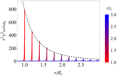
In the perfect fluid description, that assumes the fluid to remain in local equilibrium at all times, the transverse-traceless part of the stress energy tensor of the fluid reads , where is the fluid velocity and is its enthalpy density. By the interactions of the fluid with the wall, an overdense fluid shell with radial velocity builds up around the bubble wall. If the wall reaches a terminal velocity, the fluid shell settles into a self-similar profile Espinosa et al. 2010. We expect that this shell continues to propagate after the bubble wall collides with the wall of another bubble without changing its shape significantly in the collision. This behaviour was first observed for weaker transitions, , in lattice simulations Hindmarsh et al. 2017; Hindmarsh et al. 2015. For our case of very strong transitions, , we used a simplified simulation involving only the fluid and assuming extra symmetry of the system to retain only one spatial dimension as in Jinno et al. 2021.33 3 We use the integration scheme devised in Kurganov and Tadmor 2000 in order to reduce the numerical diffusion. The parameters used in the simulations are for the step in radius and a tenth of that in time. We also verified reducing the step sizes by an order of magnitude does not modify the results. We begun with simulating collisions of two planar shells and verified that they are not significantly modified and instead simply propagate onward. We next simulated the evolution of spherically symmetric fluid shells after the collision. Fig. 3 shows an illustrative example of our results. We find that the maximum of the component of the stress energy tensor scales as . This matches to the same scaling found in Jinno et al. 2021 for weak transitions and motivates us to consider for the scaling of the fluid related GW source. For comparison, we consider also which corresponds to the bulk flow model Konstandin 2018.
In principle, after the GW generation through relativistic fluid shells finishes, one would expect to enter the period of sound waves Hindmarsh et al. 2015; Hindmarsh 2018; Hindmarsh et al. 2017; Hindmarsh and Hijazi 2019 and perhaps also turbulence Roper Pol et al. 2020; Kahniashvili et al. 2021; Roper Pol et al. 2022b; Auclair et al. 2022. However, in the very strong transitions, that are our primary interest, we expect that the fluid will remain in the relativistic shells for a long time after the transition (at least until the shell radius has grown by factor). The energy carried by the inhomogeneities has then significantly diluted once the sound wave and turbulence periods begin and, therefore, we expect the main contribution on the GW spectrum in very strong transitions to arise from the relativistic fluid shells or the scalar field bubbles themselves. Thus, in the present analysis we neglect the periods of sound waves and turbulence.
| Bubbles | Fluid | ||||||
| envelope | |||||||
For certain simple forms of the function the time integral in Eq. (20) can be done analytically, which makes the simulation significantly faster. In particular, it can be done analytically if is a broken power-law with integer powers. We consider the form (10) for the efficiency factor with . Strictly speaking our results then hold for the case that . However, since the difference in for and is very small, our results give a good approximation also of the case . The pressure mainly just determines the asymptotic radius through Eqs. (7) and (6). In our simulations is an input parameter, and we perform the numerical simulations for several values of . We also assume that , which typically holds for strongly supercooled transitions, so that
| (23) |
V Results
We perform 90 simulations with simulation volume , each including at least 70 bubbles, for a range of values including both signals due to bubble walls and the surrounding fluid in each of the cases described in the previous section. From the simulations we compute the spectral shape function (19). In each case we fit the data combined from the 90 simulations with a broken power-law spectrum of the form
| (24) |
where determine the low and high frequency power-law tails of the spectrum, the width of the transition between these power-laws, while and the peak frequency and amplitude of the spectrum respectively. The resulting GW spectra are shown in Fig. 4 with the solid curves. The color coding indicates different values of .
For the solid curves in Fig. 4 the efficiency factor is directly included in the simulation as in Eqs. (21) and (22). A commonly used approximation for the effect of the efficiency factor on the GW spectrum is to multiply the spectra obtained for bubble collisions and fluid motion without any efficiency factor by and by , respectively. To check this, we have computed the amplitude of the GW spectrum in each case relative to the case that gives the largest amplitude and fitted . The data points and resulting fits for all cases are shown in Fig. 5 and the corresponding fitted values of in the last line of Table 1. We find that the effect of the efficiency factor is almost independent of the behaviour of the GW source after the collisions. In all cases our results give , showing that the often used approximation with slightly underestimates . Moreover, the results of applying the fitted efficiency factor are shown in Fig. 4 by the dashed curves. For these curves we have used the mean values given in Table 1 that are obtained by averaging over the fits with different equilibrium radius, except for the amplitude for which we use the strongest signal for each source. We see that the dashed curves agree very well with the fully numerical results shown by the solid curves. This shows that the efficiency factor does not change the shape of the GW spectrum but gives only an overall suppression factor.
To summarize, we have shown that for very strong transitions, , the GW spectrum from bubble collisions and from fluid motion, accounting for the distribution of energy between these sources, is given by
| (25) |
where the efficiency factor is given by Eq. (23). The fitted values of the parameters and are given in Table 1. For weaker transitions, , also the prefactor , given in Eq. (11), needs to be accounted for, as well as the suppression arising from heating of the fluid around the bubble wall Espinosa et al. 2010. In the limit of large wall velocity appropriate for strong transitions this reduction takes a simple form Ellis et al. 2019b
| (26) |
where .
The GW spectrum today can be obtained from (25) by accounting for the scaling of the amplitude and frequency with the scale factor Lewicki and Vaskonen 2020:44 4 Here for simplicity while red-shifting we assumed radiation dominated expansion from the transition time up to the matter-radiation equality. For a review of alternative scenarios and their impact on the spectra see Ref. Allahverdi et al. 2020.
| (27) | ||||
where denotes the dimensionless Hubble constant, Aghanim et al. 2020, and the inverse Hubble time at the transition redshifted to its value today
| (28) |
Here denotes the temperature after the transition (including reheating) and the effective number of relativistic degrees of freedom at that temperature. At scales larger than the horizon scale at the time of the transition the source is not coherent and, consequently, in standard radiation domination the slope of the spectrum changes to for Caprini et al. 2009; Cai et al. 2020.55 5 The low frequency slope is also changed by possible modifications of the expansion rate Barenboim and Park 2016; Hook et al. 2021; Gouttenoire et al. 2021 although the only scenario in which the signal is not diminished is when the modification in question is itself caused by the transition for instance through slow decay of the scalar field leading to a period of matter domination Ellis et al. 2020.
VI Conclusions
In this paper we have revisited the energy budget of strong first-order phase transitions to verify its impact on the produced gravitational wave spectra. We have gone beyond the current state-of-art by including the efficiency as a function of radius of the bubble accounting for the collision time of each point on the bubble surface. We have utilised numerical simulations randomly nucleating bubbles in a three dimensional box with periodic boundaries and used these to compute the GW spectra. This has allowed us to confirm that a simplified treatment of simply scaling entire spectra with an efficiency factor computed at some characteristic radius is accurate as the spectral shapes do not change due to the efficiency factor significantly. We did, however, find that in order to accurately describe the results the characteristic radius used in the simplified calculation should be around rather than the usually employed average bubble separation .
In each simulation we have also took into account the scaling of the GW sources after the collision in order to provide new fits for the resulting spectra from strongly supercooled transitions. The results are shown in Table 1 and, starting from strongest transitions, include bubble collision spectra for both , appropriate for gauge symmetry breaking, and , appropriate for global symmetry breaking. Going towards slightly weaker transitions, we have provided the spectrum generated by fluid motion with the scaling and assuming the fluid remains in the form of relativistic shocks after the transition. For transitions which are not extremely strong, we have show results closer to the sound wave picture in which the velocity of the fluid quickly relaxes to the speed of sound , again assuming the scaling . Finally, for illustration, we also provide fluid spectra assuming the scaling .
Taking into account that for very relativistic walls the fluid profiles are extremely peaked, we have thus show that the final GW spectrum will be indistinguishable from an even stronger transition where bubble collisions would be the main source. Only for weaker transitions where the hydrodynamical effects change the propagation speed of the fluid shells, the spectrum diverges from the spectrum arising from bubble collisions.
Acknowledgements.
This work was supported by the Spanish MINECO grants FPA2017-88915-P and SEV-2016-0588, the Spanish MICINN grants IJC2019-041533-I and PID2020-115845GB-I00/AEI/10.13039/501100011033, the grant 2017-SGR-1069 from the Generalitat de Catalunya, the Polish National Science Center grant 2018/31/D/ST2/02048, and the Polish National Agency for Academic Exchange within Polish Returns Programme under agreement PPN/PPO/2020/1/00013/U/00001. IFAE is partially funded by the CERCA program of the Generalitat de Catalunya.References
- Abbott et al. (2019) B. P. Abbott et al. (LIGO Scientific, Virgo), GWTC-1: A Gravitational-Wave Transient Catalog of Compact Binary Mergers Observed by LIGO and Virgo during the First and Second Observing Runs, Phys. Rev. X 9, 031040 (2019), arXiv:1811.12907 [astro-ph.HE] .
- Abbott et al. (2021a) R. Abbott et al. (LIGO Scientific, Virgo), GWTC-2: Compact Binary Coalescences Observed by LIGO and Virgo During the First Half of the Third Observing Run, Phys. Rev. X 11, 021053 (2021a), arXiv:2010.14527 [gr-qc] .
- Abbott et al. (2021b) R. Abbott et al. (LIGO Scientific, VIRGO), GWTC-2.1: Deep Extended Catalog of Compact Binary Coalescences Observed by LIGO and Virgo During the First Half of the Third Observing Run, (2021b), arXiv:2108.01045 [gr-qc] .
- Abbott et al. (2021c) R. Abbott et al. (LIGO Scientific, VIRGO, KAGRA), GWTC-3: Compact Binary Coalescences Observed by LIGO and Virgo During the Second Part of the Third Observing Run, (2021c), arXiv:2111.03606 [gr-qc] .
- Punturo et al. (2010) M. Punturo et al., The Einstein Telescope: A third-generation gravitational wave observatory, Class. Quant. Grav. 27, 194002 (2010).
- Hild et al. (2011) S. Hild et al., Sensitivity Studies for Third-Generation Gravitational Wave Observatories, Class. Quant. Grav. 28, 094013 (2011), arXiv:1012.0908 [gr-qc] .
- Janssen et al. (2015) G. Janssen et al., Gravitational wave astronomy with the SKA, PoS AASKA14, 037 (2015), arXiv:1501.00127 [astro-ph.IM] .
- Graham et al. (2016) P. W. Graham, J. M. Hogan, M. A. Kasevich, and S. Rajendran, Resonant mode for gravitational wave detectors based on atom interferometry, Phys. Rev. D 94, 104022 (2016), arXiv:1606.01860 [physics.atom-ph] .
- Amaro-Seoane et al. (2017) P. Amaro-Seoane et al. (LISA), Laser Interferometer Space Antenna, (2017), arXiv:1702.00786 [astro-ph.IM] .
- Graham et al. (2017) P. W. Graham, J. M. Hogan, M. A. Kasevich, S. Rajendran, and R. W. Romani (MAGIS), Mid-band gravitational wave detection with precision atomic sensors, (2017), arXiv:1711.02225 [astro-ph.IM] .
- Badurina et al. (2020) L. Badurina et al., AION: An Atom Interferometer Observatory and Network, JCAP 05, 011, arXiv:1911.11755 [astro-ph.CO] .
- El-Neaj et al. (2020) Y. A. El-Neaj et al. (AEDGE), AEDGE: Atomic Experiment for Dark Matter and Gravity Exploration in Space, EPJ Quant. Technol. 7, 6 (2020), arXiv:1908.00802 [gr-qc] .
- Bertoldi et al. (2021) A. Bertoldi et al., AEDGE: Atomic experiment for dark matter and gravity exploration in space, Exper. Astron. 51, 1417 (2021).
- Alonso et al. (2022) I. Alonso et al., Cold atoms in space: community workshop summary and proposed road-map, EPJ Quant. Technol. 9, 30 (2022), arXiv:2201.07789 [astro-ph.IM] .
- Badurina et al. (2021) L. Badurina, O. Buchmueller, J. Ellis, M. Lewicki, C. McCabe, and V. Vaskonen, Prospective sensitivities of atom interferometers to gravitational waves and ultralight dark matter, Phil. Trans. A. Math. Phys. Eng. Sci. 380, 20210060 (2021), arXiv:2108.02468 [gr-qc] .
- Lewicki and Vaskonen (2021a) M. Lewicki and V. Vaskonen, Impact of LIGO-Virgo binaries on gravitational wave background searches, (2021a), arXiv:2111.05847 [astro-ph.CO] .
- Arzoumanian et al. (2020) Z. Arzoumanian et al. (NANOGrav), The NANOGrav 12.5 yr Data Set: Search for an Isotropic Stochastic Gravitational-wave Background, Astrophys. J. Lett. 905, L34 (2020), arXiv:2009.04496 [astro-ph.HE] .
- Goncharov et al. (2021) B. Goncharov et al., On the Evidence for a Common-spectrum Process in the Search for the Nanohertz Gravitational-wave Background with the Parkes Pulsar Timing Array, Astrophys. J. Lett. 917, L19 (2021), arXiv:2107.12112 [astro-ph.HE] .
- Chen et al. (2021) S. Chen et al., Common-red-signal analysis with 24-yr high-precision timing of the European Pulsar Timing Array: inferences in the stochastic gravitational-wave background search, Mon. Not. Roy. Astron. Soc. 508, 4970 (2021), arXiv:2110.13184 [astro-ph.HE] .
- Antoniadis et al. (2022) J. Antoniadis et al., The International Pulsar Timing Array second data release: Search for an isotropic gravitational wave background, Mon. Not. Roy. Astron. Soc. 510, 4873 (2022), arXiv:2201.03980 [astro-ph.HE] .
- Ellis and Lewicki (2021) J. Ellis and M. Lewicki, Cosmic String Interpretation of NANOGrav Pulsar Timing Data, Phys. Rev. Lett. 126, 041304 (2021), arXiv:2009.06555 [astro-ph.CO] .
- Blasi et al. (2021) S. Blasi, V. Brdar, and K. Schmitz, Has NANOGrav found first evidence for cosmic strings?, Phys. Rev. Lett. 126, 041305 (2021), arXiv:2009.06607 [astro-ph.CO] .
- Vaskonen and Veermäe (2021) V. Vaskonen and H. Veermäe, Did NANOGrav see a signal from primordial black hole formation?, Phys. Rev. Lett. 126, 051303 (2021), arXiv:2009.07832 [astro-ph.CO] .
- De Luca et al. (2021) V. De Luca, G. Franciolini, and A. Riotto, NANOGrav Data Hints at Primordial Black Holes as Dark Matter, Phys. Rev. Lett. 126, 041303 (2021), arXiv:2009.08268 [astro-ph.CO] .
- Nakai et al. (2021) Y. Nakai, M. Suzuki, F. Takahashi, and M. Yamada, Gravitational Waves and Dark Radiation from Dark Phase Transition: Connecting NANOGrav Pulsar Timing Data and Hubble Tension, Phys. Lett. B 816, 136238 (2021), arXiv:2009.09754 [astro-ph.CO] .
- Ratzinger and Schwaller (2021) W. Ratzinger and P. Schwaller, Whispers from the dark side: Confronting light new physics with NANOGrav data, SciPost Phys. 10, 047 (2021), arXiv:2009.11875 [astro-ph.CO] .
- Kohri and Terada (2021) K. Kohri and T. Terada, Solar-Mass Primordial Black Holes Explain NANOGrav Hint of Gravitational Waves, Phys. Lett. B 813, 136040 (2021), arXiv:2009.11853 [astro-ph.CO] .
- Vagnozzi (2021) S. Vagnozzi, Implications of the NANOGrav results for inflation, Mon. Not. Roy. Astron. Soc. 502, L11 (2021), arXiv:2009.13432 [astro-ph.CO] .
- Neronov et al. (2021) A. Neronov, A. Roper Pol, C. Caprini, and D. Semikoz, NANOGrav signal from magnetohydrodynamic turbulence at the QCD phase transition in the early Universe, Phys. Rev. D 103, 041302 (2021), arXiv:2009.14174 [astro-ph.CO] .
- Blanco-Pillado et al. (2021) J. J. Blanco-Pillado, K. D. Olum, and J. M. Wachter, Comparison of cosmic string and superstring models to NANOGrav 12.5-year results, Phys. Rev. D 103, 103512 (2021), arXiv:2102.08194 [astro-ph.CO] .
- Wang (2022) D. Wang, Squeezing Cosmological Phase Transitions with International Pulsar Timing Array, (2022), arXiv:2201.09295 [astro-ph.CO] .
- Roper Pol et al. (2022a) A. Roper Pol, C. Caprini, A. Neronov, and D. Semikoz, Gravitational wave signal from primordial magnetic fields in the Pulsar Timing Array frequency band, Phys. Rev. D 105, 123502 (2022a), arXiv:2201.05630 [astro-ph.CO] .
- Ferreira et al. (2022) R. Z. Ferreira, A. Notari, O. Pujolas, and F. Rompineve, Gravitational Waves from Domain Walls in Pulsar Timing Array Datasets, (2022), arXiv:2204.04228 [astro-ph.CO] .
- Caprini et al. (2016) C. Caprini et al., Science with the space-based interferometer eLISA. II: Gravitational waves from cosmological phase transitions, JCAP 04, 001, arXiv:1512.06239 [astro-ph.CO] .
- Caprini et al. (2020) C. Caprini et al., Detecting gravitational waves from cosmological phase transitions with LISA: an update, JCAP 03, 024, arXiv:1910.13125 [astro-ph.CO] .
- Auclair et al. (2020) P. Auclair et al., Probing the gravitational wave background from cosmic strings with LISA, JCAP 04, 034, arXiv:1909.00819 [astro-ph.CO] .
- Bartolo et al. (2016) N. Bartolo et al., Science with the space-based interferometer LISA. IV: Probing inflation with gravitational waves, JCAP 12, 026, arXiv:1610.06481 [astro-ph.CO] .
- Coleman (1977) S. R. Coleman, The Fate of the False Vacuum. 1. Semiclassical Theory, Phys. Rev. D 15, 2929 (1977), [Erratum: Phys.Rev.D 16, 1248 (1977)].
- Kosowsky and Turner (1993) A. Kosowsky and M. S. Turner, Gravitational radiation from colliding vacuum bubbles: envelope approximation to many bubble collisions, Phys. Rev. D 47, 4372 (1993), arXiv:astro-ph/9211004 .
- Kamionkowski et al. (1994) M. Kamionkowski, A. Kosowsky, and M. S. Turner, Gravitational radiation from first order phase transitions, Phys. Rev. D 49, 2837 (1994), arXiv:astro-ph/9310044 .
- Hindmarsh and Hijazi (2019) M. Hindmarsh and M. Hijazi, Gravitational waves from first order cosmological phase transitions in the Sound Shell Model, JCAP 12, 062, arXiv:1909.10040 [astro-ph.CO] .
- Cutting et al. (2020) D. Cutting, M. Hindmarsh, and D. J. Weir, Vorticity, kinetic energy, and suppressed gravitational wave production in strong first order phase transitions, Phys. Rev. Lett. 125, 021302 (2020), arXiv:1906.00480 [hep-ph] .
- Lewicki and Vaskonen (2020) M. Lewicki and V. Vaskonen, Gravitational wave spectra from strongly supercooled phase transitions, Eur. Phys. J. C 80, 1003 (2020), arXiv:2007.04967 [astro-ph.CO] .
- Lewicki and Vaskonen (2021b) M. Lewicki and V. Vaskonen, Gravitational waves from colliding vacuum bubbles in gauge theories, Eur. Phys. J. C 81, 437 (2021b), [Erratum: Eur.Phys.J.C 81, 1077 (2021)], arXiv:2012.07826 [astro-ph.CO] .
- Jinno et al. (2021) R. Jinno, T. Konstandin, and H. Rubira, A hybrid simulation of gravitational wave production in first-order phase transitions, JCAP 04, 014, arXiv:2010.00971 [astro-ph.CO] .
- Dahl et al. (2022) J. Dahl, M. Hindmarsh, K. Rummukainen, and D. J. Weir, Decay of acoustic turbulence in two dimensions and implications for cosmological gravitational waves, Phys. Rev. D 106, 063511 (2022), arXiv:2112.12013 [gr-qc] .
- Cutting et al. (2022) D. Cutting, E. Vilhonen, and D. J. Weir, Droplet collapse during strongly supercooled transitions, Phys. Rev. D 106, 103524 (2022), arXiv:2204.03396 [astro-ph.CO] .
- Jinno and Takimoto (2017) R. Jinno and M. Takimoto, Probing a classically conformal B-L model with gravitational waves, Phys. Rev. D 95, 015020 (2017), arXiv:1604.05035 [hep-ph] .
- Iso et al. (2017) S. Iso, P. D. Serpico, and K. Shimada, QCD-Electroweak First-Order Phase Transition in a Supercooled Universe, Phys. Rev. Lett. 119, 141301 (2017), arXiv:1704.04955 [hep-ph] .
- Marzola et al. (2017) L. Marzola, A. Racioppi, and V. Vaskonen, Phase transition and gravitational wave phenomenology of scalar conformal extensions of the Standard Model, Eur. Phys. J. C 77, 484 (2017), arXiv:1704.01034 [hep-ph] .
- Prokopec et al. (2019) T. Prokopec, J. Rezacek, and B. Świeżewska, Gravitational waves from conformal symmetry breaking, JCAP 02, 009, arXiv:1809.11129 [hep-ph] .
- Marzo et al. (2019) C. Marzo, L. Marzola, and V. Vaskonen, Phase transition and vacuum stability in the classically conformal B–L model, Eur. Phys. J. C 79, 601 (2019), arXiv:1811.11169 [hep-ph] .
- Baratella et al. (2019) P. Baratella, A. Pomarol, and F. Rompineve, The Supercooled Universe, JHEP 03, 100, arXiv:1812.06996 [hep-ph] .
- Von Harling et al. (2020) B. Von Harling, A. Pomarol, O. Pujolàs, and F. Rompineve, Peccei-Quinn Phase Transition at LIGO, JHEP 04, 195, arXiv:1912.07587 [hep-ph] .
- Aoki and Kubo (2020) M. Aoki and J. Kubo, Gravitational waves from chiral phase transition in a conformally extended standard model, JCAP 04, 001, arXiv:1910.05025 [hep-ph] .
- Delle Rose et al. (2020) L. Delle Rose, G. Panico, M. Redi, and A. Tesi, Gravitational Waves from Supercool Axions, JHEP 04, 025, arXiv:1912.06139 [hep-ph] .
- Wang et al. (2020) X. Wang, F. P. Huang, and X. Zhang, Phase transition dynamics and gravitational wave spectra of strong first-order phase transition in supercooled universe, JCAP 05, 045, arXiv:2003.08892 [hep-ph] .
- Ellis et al. (2020) J. Ellis, M. Lewicki, and V. Vaskonen, Updated predictions for gravitational waves produced in a strongly supercooled phase transition, JCAP 11, 020, arXiv:2007.15586 [astro-ph.CO] .
- Baldes et al. (2021) I. Baldes, Y. Gouttenoire, and F. Sala, String Fragmentation in Supercooled Confinement and Implications for Dark Matter, JHEP 04, 278, arXiv:2007.08440 [hep-ph] .
- Baldes et al. (2022) I. Baldes, Y. Gouttenoire, F. Sala, and G. Servant, Supercool composite Dark Matter beyond 100 TeV, JHEP 07, 084, arXiv:2110.13926 [hep-ph] .
- Lewicki et al. (2021) M. Lewicki, O. Pujolàs, and V. Vaskonen, Escape from supercooling with or without bubbles: gravitational wave signatures, Eur. Phys. J. C 81, 857 (2021), arXiv:2106.09706 [astro-ph.CO] .
- Grojean and Servant (2007) C. Grojean and G. Servant, Gravitational Waves from Phase Transitions at the Electroweak Scale and Beyond, Phys. Rev. D 75, 043507 (2007), arXiv:hep-ph/0607107 .
- Dorsch et al. (2014) G. C. Dorsch, S. J. Huber, and J. M. No, Cosmological Signatures of a UV-Conformal Standard Model, Phys. Rev. Lett. 113, 121801 (2014), arXiv:1403.5583 [hep-ph] .
- Huang et al. (2016) P. Huang, A. J. Long, and L.-T. Wang, Probing the Electroweak Phase Transition with Higgs Factories and Gravitational Waves, Phys. Rev. D 94, 075008 (2016), arXiv:1608.06619 [hep-ph] .
- Artymowski et al. (2017) M. Artymowski, M. Lewicki, and J. D. Wells, Gravitational wave and collider implications of electroweak baryogenesis aided by non-standard cosmology, JHEP 03, 066, arXiv:1609.07143 [hep-ph] .
- Vaskonen (2017) V. Vaskonen, Electroweak baryogenesis and gravitational waves from a real scalar singlet, Phys. Rev. D 95, 123515 (2017), arXiv:1611.02073 [hep-ph] .
- Dorsch et al. (2017) G. C. Dorsch, S. J. Huber, T. Konstandin, and J. M. No, A Second Higgs Doublet in the Early Universe: Baryogenesis and Gravitational Waves, JCAP 05, 052, arXiv:1611.05874 [hep-ph] .
- Ellis et al. (2019a) J. Ellis, M. Lewicki, and J. M. No, On the Maximal Strength of a First-Order Electroweak Phase Transition and its Gravitational Wave Signal, JCAP 04, 003, arXiv:1809.08242 [hep-ph] .
- Beniwal et al. (2019) A. Beniwal, M. Lewicki, M. White, and A. G. Williams, Gravitational waves and electroweak baryogenesis in a global study of the extended scalar singlet model, JHEP 02, 183, arXiv:1810.02380 [hep-ph] .
- Fairbairn et al. (2019) M. Fairbairn, E. Hardy, and A. Wickens, Hearing without seeing: gravitational waves from hot and cold hidden sectors, JHEP 07, 044, arXiv:1901.11038 [hep-ph] .
- Ellis et al. (2019b) J. Ellis, M. Lewicki, J. M. No, and V. Vaskonen, Gravitational wave energy budget in strongly supercooled phase transitions, JCAP 06, 024, arXiv:1903.09642 [hep-ph] .
- Lewicki et al. (2022a) M. Lewicki, M. Merchand, and M. Zych, Electroweak bubble wall expansion: gravitational waves and baryogenesis in Standard Model-like thermal plasma, JHEP 02, 017, arXiv:2111.02393 [astro-ph.CO] .
- Cai and Wang (2021) R.-G. Cai and S.-J. Wang, Effective picture of bubble expansion, JCAP 03, 096, arXiv:2011.11451 [astro-ph.CO] .
- Lewicki et al. (2022b) M. Lewicki, V. Vaskonen, and H. Veermäe, Bubble dynamics in fluids with N-body simulations, Phys. Rev. D 106, 103501 (2022b), arXiv:2205.05667 [astro-ph.CO] .
- Bodeker and Moore (2009) D. Bodeker and G. D. Moore, Can electroweak bubble walls run away?, JCAP 05, 009, arXiv:0903.4099 [hep-ph] .
- Bodeker and Moore (2017) D. Bodeker and G. D. Moore, Electroweak Bubble Wall Speed Limit, JCAP 05, 025, arXiv:1703.08215 [hep-ph] .
- Azatov and Vanvlasselaer (2021) A. Azatov and M. Vanvlasselaer, Bubble wall velocity: heavy physics effects, JCAP 01, 058, arXiv:2010.02590 [hep-ph] .
- Gouttenoire et al. (2022) Y. Gouttenoire, R. Jinno, and F. Sala, Friction pressure on relativistic bubble walls, JHEP 05, 004, arXiv:2112.07686 [hep-ph] .
- Höche et al. (2021) S. Höche, J. Kozaczuk, A. J. Long, J. Turner, and Y. Wang, Towards an all-orders calculation of the electroweak bubble wall velocity, JCAP 03, 009, arXiv:2007.10343 [hep-ph] .
- Barroso Mancha et al. (2021) M. Barroso Mancha, T. Prokopec, and B. Swiezewska, Field-theoretic derivation of bubble-wall force, JHEP 01, 070, arXiv:2005.10875 [hep-th] .
- Espinosa et al. (2010) J. R. Espinosa, T. Konstandin, J. M. No, and G. Servant, Energy Budget of Cosmological First-order Phase Transitions, JCAP 06, 028, arXiv:1004.4187 [hep-ph] .
- Jinno et al. (2019) R. Jinno, H. Seong, M. Takimoto, and C. M. Um, Gravitational waves from first-order phase transitions: Ultra-supercooled transitions and the fate of relativistic shocks, JCAP 10, 033, arXiv:1905.00899 [astro-ph.CO] .
- Hindmarsh et al. (2017) M. Hindmarsh, S. J. Huber, K. Rummukainen, and D. J. Weir, Shape of the acoustic gravitational wave power spectrum from a first order phase transition, Phys. Rev. D 96, 103520 (2017), [Erratum: Phys.Rev.D 101, 089902 (2020)], arXiv:1704.05871 [astro-ph.CO] .
- Hindmarsh et al. (2015) M. Hindmarsh, S. J. Huber, K. Rummukainen, and D. J. Weir, Numerical simulations of acoustically generated gravitational waves at a first order phase transition, Phys. Rev. D 92, 123009 (2015), arXiv:1504.03291 [astro-ph.CO] .
- Kurganov and Tadmor (2000) A. Kurganov and E. Tadmor, New high-resolution central schemes for nonlinear conservation laws and convection–diffusion equations, Journal of Computational Physics 160, 241 (2000).
- Konstandin (2018) T. Konstandin, Gravitational radiation from a bulk flow model, JCAP 03, 047, arXiv:1712.06869 [astro-ph.CO] .
- Hindmarsh (2018) M. Hindmarsh, Sound shell model for acoustic gravitational wave production at a first-order phase transition in the early Universe, Phys. Rev. Lett. 120, 071301 (2018), arXiv:1608.04735 [astro-ph.CO] .
- Roper Pol et al. (2020) A. Roper Pol, S. Mandal, A. Brandenburg, T. Kahniashvili, and A. Kosowsky, Numerical simulations of gravitational waves from early-universe turbulence, Phys. Rev. D 102, 083512 (2020), arXiv:1903.08585 [astro-ph.CO] .
- Kahniashvili et al. (2021) T. Kahniashvili, A. Brandenburg, G. Gogoberidze, S. Mandal, and A. Roper Pol, Circular polarization of gravitational waves from early-Universe helical turbulence, Phys. Rev. Res. 3, 013193 (2021), arXiv:2011.05556 [astro-ph.CO] .
- Roper Pol et al. (2022b) A. Roper Pol, S. Mandal, A. Brandenburg, and T. Kahniashvili, Polarization of gravitational waves from helical MHD turbulent sources, JCAP 04 (04), 019, arXiv:2107.05356 [gr-qc] .
- Auclair et al. (2022) P. Auclair, C. Caprini, D. Cutting, M. Hindmarsh, K. Rummukainen, D. A. Steer, and D. J. Weir, Generation of gravitational waves from freely decaying turbulence, JCAP 09, 029, arXiv:2205.02588 [astro-ph.CO] .
- Allahverdi et al. (2020) R. Allahverdi et al., The First Three Seconds: a Review of Possible Expansion Histories of the Early Universe 10.21105/astro.2006.16182 (2020), arXiv:2006.16182 [astro-ph.CO] .
- Aghanim et al. (2020) N. Aghanim et al. (Planck), Planck 2018 results. VI. Cosmological parameters, Astron. Astrophys. 641, A6 (2020), [Erratum: Astron.Astrophys. 652, C4 (2021)], arXiv:1807.06209 [astro-ph.CO] .
- Caprini et al. (2009) C. Caprini, R. Durrer, T. Konstandin, and G. Servant, General Properties of the Gravitational Wave Spectrum from Phase Transitions, Phys. Rev. D 79, 083519 (2009), arXiv:0901.1661 [astro-ph.CO] .
- Cai et al. (2020) R.-G. Cai, S. Pi, and M. Sasaki, Universal infrared scaling of gravitational wave background spectra, Phys. Rev. D 102, 083528 (2020), arXiv:1909.13728 [astro-ph.CO] .
- Barenboim and Park (2016) G. Barenboim and W.-I. Park, Gravitational waves from first order phase transitions as a probe of an early matter domination era and its inverse problem, Phys. Lett. B 759, 430 (2016), arXiv:1605.03781 [astro-ph.CO] .
- Hook et al. (2021) A. Hook, G. Marques-Tavares, and D. Racco, Causal gravitational waves as a probe of free streaming particles and the expansion of the Universe, JHEP 02, 117, arXiv:2010.03568 [hep-ph] .
- Gouttenoire et al. (2021) Y. Gouttenoire, G. Servant, and P. Simakachorn, Kination cosmology from scalar fields and gravitational-wave signatures, (2021), arXiv:2111.01150 [hep-ph] .