Analysis of adiabatic trapping phenomena for quasi-integrable area-preserving maps in the presence of time-dependent exciters
Abstract
In this paper, new results concerning the phenomenon of adiabatic trapping into resonance for a class of quasi-integrable maps with a time-dependent exciter are presented and discussed in detail. The applicability of the results about trapping efficiency for Hamiltonian systems to the maps considered is proven by using perturbation theory. This allows determining explicit scaling laws for the trapping properties. These findings represent a generalization of previous results obtained for the case of quasi-integrable maps with parametric modulation as well as an extension of the work by Neishtadt et al. on a restricted class of quasi-integrable systems with time-dependent exciters.
1 Introduction
The adiabatic theory for Hamiltonian systems is a key breakthrough towards an understanding of the effects of slow parametric modulation on the dynamics. The concept of adiabatic invariant allows the long-term evolution of the system to be predicted and the fundamental properties of the action variables to be highlighted upon averaging over the fast variables [1, 2]. The theory has been well developed for systems with one degree of freedom [3, 4, 5, 6, 7], but the extension of some analytical results to multi-dimensional systems or to symplectic maps [8] has to cope with the issues generated by small denominators and the ubiquitous presence of resonances in phase space [9, 10]. For these reasons, such an extension is still an open problem.
Recently, the possibility of a controlled manipulation of the phase space by means of an adiabatic change of a parameter opened the road-map to new applications in accelerator and plasma physics [11, 12, 13, 14, 15, 16]. In particular, the adiabatic transport performed by means of nonlinear resonance trapping allows to manipulate a charged particle distribution so to minimize the particle losses during the beam extraction process in a circular accelerator. Furthermore, the control of the beam emittance can be obtained by a similar approach [17, 18, 19]. The experimental procedures [17, 18, 19] require a very precise control of the efficiency of the adiabatic trapping into resonances [7, 20, 21], as well as of the phase-space change during the adiabatic transport when the parametric modulation is introduced by means of an external perturbation. All these processes can be represented by multi-dimensional Hamiltonian systems or symplectic maps [22].
In this paper, we consider the problem of obtaining an accurate estimate of the resonance-trapping efficiency and of the phase-space transport for a given distribution of initial conditions in the case of polynomial symplectic maps when a time-dependent periodic perturbation is present. The perturbation frequency and amplitude are adiabatically changed. We show that the concept of interpolating Hamiltonian can be applied to derive the scaling laws of the main parameters of the map, i.e. the perturbation amplitude, and the nonlinearity coefficients. In this way, we obtain explicit analytical estimates for the trapping and transport efficiencies, thus generalizing the analytical results obtained for Hamiltonian systems. The accuracy of the proposed estimates has been verified by means of extensive numerical simulations of different study cases. Furthermore, we study the limits of the adiabatic approximation for the observed phenomena, and of the validity of our results. Note that the modulation of the external perturbation parameters is realized according to procedures that could open the way to new applications in the field of accelerator physics, in view of devising novel beam manipulations.
The paper is organized as follows: in Section 2 we recall some theoretical results of the adiabatic theory that are needed to measure the resonance-trapping phenomenon, and we introduce the map models. In Section 3 we perform a detailed analysis of the phase-space evolution during the trapping process, whereas in Section 4 we discuss the results of detailed numerical simulations about the evolution of a particle distribution, comparing the dynamics of the interpolating Hamiltonian with that of the corresponding symplectic maps. In section 5, a more complex model is presented and discussed to show that in spite of its features, the theory works well in generic systems. Finally, some conclusions are drawn in Section 6, and some detailed computations of the the perturbation-theory calculations for a Hamiltonian system with a time-dependent exciter and the minimum action for which trapping occurs are reported in Appendix A, and B, respectively.
2 Theory
2.1 Generalities
Phenomena occurring when a Hamiltonian system is slowly modulated have been widely studied in the framework of adiabatic theory [23, 4]. As the modulation of the Hamiltonian changes the shape of the separatrices in phase space, the trajectories can cross separatrices and enter into different stable regions that are associated with nonlinear resonances. The probability of the separatrix crossing, which is described by a random process in the adiabatic limit, can be computed as well as the change of adiabatic invariant due to the crossing [23, 4].
Let us consider a Hamiltonian , where the parameter is slowly modulated and whose phase space is sketched in Fig. 1. If we consider an initial condition that lies in Region , the transition probability into Region or of phase space is given by [23]
| (1) |
where
| (2) |
with the area of the region , the boundary of region , and the value of when the separatrix is crossed. We remark that in case , then is set to zero, whereas when then is set to unity.
When a separatrix is crossed, the adiabatic invariant is expected to change according to the area difference between the two regions at the crossing time, so that just after the crossing into a region of area , we have . However, this value is exact only if the modulation is perfectly adiabatic, i.e. it is infinitely slow. A correction to the value of the new action can be found following [4], and it is a random value, whose distribution depends on the random variable , being the difference between the energy of a particle and that of the separatrix. The value of can be considered a random variable in the adiabatic limit, due to its extreme sensitivity to the initial condition of the action.
The adiabatic trapping into resonances has been studied in various works [23, 24] to show the possibility of transport in phase space when some system’s parameters are slowly modulated. This phenomenon suggests possible applications in different fields and, in particular, in accelerator physics where the Multi-Turn Extraction has been proposed [25] and successfully made an operational beam manipulation at the CERN Proton Synchrotron [26, 17]. In this case, an extension of the results of adiabatic theory to quasi-integrable area-preserving maps has been considered, and analogous probabilities (1) to be captured in a resonance can be computed [22] when the Poincaré–Birkhoff theorem [27] can be applied to prove the existence of stable islands in phase space. The properties of such resonance islands for polynomial Hénon-like maps [28] have been studied in [29] and the possibility of performing an adiabatic trapping into a resonance has been studied by modulating the linear frequency at the elliptic fixed point [22]. In this paper we extend the previous results by considering the adiabatic trapping in area-preserving maps when we introduce a time-modulated external sinusoidal term in the dynamics, with amplitude proportional to , and whose frequency is adiabatically changed to cross a resonance with the unperturbed frequency of the system. This external forcing is particularly relevant for applications, as it mimics the effect of a transverse kicker on the charged particle dynamics in a circular accelerator (see, e.g. [30, 31, 32, 33, 34, 35] and references therein). Furthermore, it would allow extending the possibility to perform an efficient beam trapping into stable islands even when the unperturbed frequencies of the system cannot be modulated. This might be the case e.g. in a circular particle accelerator in the presence of space charge effects that impose a special choice of linear tunes.
2.2 The models used
We consider a Hénon-like symplectic map of the form
| (3) |
where is a rotation matrix of an angle , is the iteration number, , and the dynamics is perturbed by a modulated kick of amplitude whose frequency is close to a resonance condition . We remark that when , the fixed point at the origin of the unperturbed system becomes an elliptic periodic orbit of period , and the linearized frequencies depend on the perturbation strength, so that they are adiabatically modulated. This is not the case when , which is also interesting for applications. We shall consider explicitly these two cases.
The Birkhoff Normal Form theory allows a relationship between the map of Eq. (3) and the Hamiltonian [29]
| (4) |
to be established.
In particular, from Eq. (3) we can derive the Normal Form Hamiltonian
| (5) |
where are detuning terms, obtained from the non-resonant Normal Form, while is the Fourier component of the th harmonic, which is the only one remaining when . We remark that the dependence of on the is in the form of a polynomial, and the scaling laws have been derived in [29]. For instance, in the case of one has , where
| (6) |
If the Hamiltonian (4) is averaged on the resonance, one obtains an expression of the same form as Eq. (5), i.e.
| (7) |
where we have the same Fourier coefficient that appears from the expansion of on the resonant harmonic, and is a polynomial function of the .
From these two expressions, it is possible to evaluate the relation between the corresponding parameters, i.e. and , which enables applying the analytical results valid for the Hamiltonian system to the corresponding polynomial symplectic map of the form (3).
Let be the action-angle variables for the map defined by the perturbation series. The frequency of the angle dynamics can be written in the form [29]
| (8) |
while from the Hamiltonian (4), which is expressed in terms of the action-angle variables , we obtain
| (9) |
where stands for the average over the variable .
If a single detuning term of order is considered and a single term is present in the system under study, and (and similarly for ), then one can assume that and only the action variables need to be re-scaled to ensure the same frequency variation with action for the two systems under consideration. If , then from the expression
| (10) |
we derive
| (11) |
In the more general case in which several detuning terms are considered, but a single term is present, we have (and similarly for ). The approach consists of re-scaling instead of the action, which would then give the solution
| (12) |
thus making the frequency variation the same for both systems also in this case.
For and , the outlined approach gives
| (13) |
and we still need to match the strength of the time-dependent perturbation, which is proportional to , so that
| (14) |
In the numerical simulations, we set and , finding from the computation of the Fourier coefficient by means of the perturbation theory, which is found in Appendix A).
Performing analogous computations for and (see Appendix A), the coefficient can be computed and by comparing it with the corresponding coefficient for the case one determines the different scale of the perturbation strength in the two cases, namely
| (15) |
According to the parameters used in the simulations ( and ) we obtain , and the values of are the same order of magnitude for the two cases. We thus expect comparable results for the resonance-trapping phenomenon.
3 Analysis of the trapping process
The numerical studies carried out to analyze the phenomenology of the trapping process have been performed with the map model of Eq. (3) as well as the Hamiltonian of Eq. (4) in order to establish conditions under which the adiabatic resonance trapping for the modulated symplectic map can be described by the analytical results for Hamiltonian systems in a neighborhood of the elliptic fixed point.

The main aspect relevant for applications is to investigate which initial conditions are trapped in the resonance and transported in phase space. For this purpose, we determine whether a trajectory is in the resonance islands of the frozen map, relying on the result that the main Fourier component of an orbit in a resonance island corresponds to the resonant tune . We used high-accuracy algorithms for the computation of the main Fourier component [36, 37] to perform the correct identification of the trapped orbits. In Fig. 2 (top) we show an example of the main frequency for a set of orbits with initial conditions of the form whose evolution under the Hamiltonian model (4) is evaluated by freezing the time dependence of the system parameters (the corresponding phase-space portrait is shown in the bottom plot of Fig. 2). A dependence of the main frequency as a function of is clearly visible. Note also that the region of constant frequency corresponds to the so-called phase-locking, which occurs when the dynamics is inside a stable island. A sudden jump in frequency can be observed at , which corresponds to an initial condition on the hyperbolic fixed point.
In the following, the concept of trapping fraction will be used in view of studying and qualifying the efficiency of trapping protocols. Given a distribution of initial conditions, the trapping fraction is defined as the ratio of the trapped particles to those in the initial distribution. It is clear that the definition depends on the distribution selected for the initial conditions. For our analysis, it is important to record the original and final regions of the particles: this is made by defining the symbol , where stands for the region (or regions) from which the initial conditions are taken and stands for the region in which they are trapped. We remark that the definition of the region from which particles are taken or trapped is based on the phase space topology (such as that visible in Fig. 2), at the end of the first stage of the trapping protocol described in the next section.
3.1 Hamiltonian models
To study the phase space of the Hamiltonian of Eq. (4), it is convenient to use the Poincaré map (see the bottom plot of Fig. 2 for an example of phase-space portrait). When either or are changed, the separatrices move in phase space changing the enclosed area, while keeping the same topology for sufficiently small and sufficiently close to the resonance. To describe the phenomenology, the third-order resonance is selected, but the concepts used can be generalized to any resonance order.
According to [23], when the system parameters are adiabatically modulated, the trapping of the orbits into the stable islands and the adiabatic transport are possible. To optimize the trapping probability, we propose a protocol divided into two steps. In the first one, the perturbation frequency is kept constant at a value , near the th-order resonance, while the exciter is slowly switched on, increasing its strength from to the final value . In the second stage, the exciter strength is kept fixed at , and the frequency is modulated from to . Both modulations are performed by means of a linear variation in time steps.
In the first step, as increases, the area of the resonance islands increases, thus trapping all orbits that cross the separatrix according to Eq. (1). The phase space can be divided in three regions (see Fig. 2, bottom): the inner region (Region I) encloses the origin and is limited by the inner part of the separatrices, the resonance region (Region II) made of the stable islands, and the outer region (Region III) from the outer part of the separatrix to infinity. The areas of Region I and II are shown in Fig. 3 as a function of the exciter strength (top) and the distance from the resonance (bottom).
We remark that is always decreasing with , whereas is increasing up to . Therefore, since has a maximum at , the Region III area is increasing when .
In the case of an ensemble of initial conditions chosen in Region I, for adiabatic theory ensures that every orbit crossing the inner separatrix is trapped in the resonance, i.e. in Region II. When , as both Region II and III areas are increasing, a fraction of orbits will enter into Region III according to Eq. (1). These observations are essential for engineering the variation of the system parameters in order to control the trapping and transport phenomena, which is essential for devising successful applications. An example of the behavior described above is shown in Fig. 4 in which the evolution of a set of initial conditions under the dynamics generated by using the protocol for trapping and transport described above is shown.
Both rows show the evolution of an ensemble of initial conditions under the same dynamics generated by and the colors are used to indicate which region the initial conditions are trapped into. The trapping and transport phenomena are clearly visible, thus indicating that the proposed protocol works efficiently. Between the two rows, the distribution of initial conditions is changed. In the top row, the larger amplitude of the initial conditions is such that an annulus exists in which initial conditions can be trapped either in Region I or II. On the other hand, the smaller extent of the initial distribution in the bottom row removes this phenomenon and there is a clear separation between particles that will be trapped in Region I or II. We remark also that the initial conditions at large amplitude in the top row contribute to a larger surface of the transported islands and core.
According to adiabatic theory [23], all particles whose orbit encloses an area at the end of the first stage satisfying will be trapped in the resonance, whereas the particles with will remain in Region I. Furthermore, assuming that the orbits in the excluded region are very close to the origin, we can estimate the average distance from the origin at which the resonance trapping occurs by . Fig. 5 shows the remarkable agreement between the minimum enclosed area of the trapped orbits and the final area as function of .
If , the particles that enclose an area satisfying will be found in the external Region III at the end of the first stage. Therefore, the distribution of initial conditions around the origin can be divided in three parts: the part close to the origin that remains in Region I, the part trapped in the resonance i.e. in Region II, and the part that is or enters into Region III.
During the second phase, the exciter frequency is varied to move the resonance in phase space and thus performing the adiabatic transport of the trapped initial conditions. As shown in Fig. 3 (bottom), both Region I and II increase their area so that no further trapping of orbits close to the origin nor any detrapping from the resonance region are expected. Conversely, the orbits in Region III will enter either Region II or I according to the probabilities (see Eq. (1)) that are calculated at the time when the separatrix crossing occurs [23].
We remark that for the systems under consideration, the dependence of on the system parameters is so smooth that approximating the derivatives of at the time of the actual separatrix crossing, which is needed to compute the trapping probabilities, with a finite difference is an excellent approximation.
The situation is radically different when one considers as it can be seen in Fig. 6, where the areas of the center (Region I) and of the islands (Region II) are shown as a function of .
Indeed, in this case, is decreasing only for a small interval of around zero, and then it increases, while increases monotonically, similarly to the sum of the two areas. This implies that there is no possibility for trapping in Region III. Furthermore, the initial conditions in Region III will be trapped either in Region I or II according to Eq. (1).
3.2 Map models
To investigate the same phenomena using the map (3) we need to provide an appropriate framework that allows determining the areas of the various regions as done for the Hamiltonian models.
We remark that , inspected for different models follows the scaling laws and outlined in [29]. In fact, if we assume that close to a hyperbolic fixed point with action-angle coordinates , we can approximate the motion using the pendulum-like Hamiltonian
| (16) |
where is proportional to , , and reads
| (17) |
and since , we obtain
| (18) |
and this scaling law is shown in Fig. 7, where the numerical evaluation of is compared with the scaling law (18) as a function of (top) and (bottom).
Figure 7 (top) shows clearly that the fit fails for large values of for . We remark that the Hamiltonian of Eq. (16) is approximated, hence a better estimate of can be found by starting from the following Hamiltonian i.e.
| (19) |
and approximating the coefficient of the resonant term with the first-order series expansion in , which gives
| (20) |
The area enclosed by the separatrix is then given by the integral
| (21) |
where is the value of given in Eq. (17), while , i.e. . The expansion of (21) reads [38]
| (22) |
which corresponds to a dependence, in
| (23) |
where , and can be determined via a fitting process. This estimate, shown in Fig. 7 (top) as “improved fit”, is in good agreement with the data.
In Fig. 5, we see the excellent agreement between the minimum radius for which the trapping occurs, and the area of Region I at the end of the first phase of the modulation for the map model, which is a further indication of the validity of the proposed approach. This is also confirmed by the results shown in Fig. 8, where the fraction of particles trapped in Region from Region is shown for different models as a function of . The predictions from Eq. (1) are also shown and a very good agreement is observed. Moreover, in Fig. 5 we show that a fit function of the form fits well the data for , where is a form factor that tends to a constant value for large values of , and that reads
| (24) |
and this model is fully consistent with the analysis of the minimum trapping action presented in Appendix B. We remark that the approach presented in the Appendix finds, as estimate of the minimum trapping action, the action of the hyperbolic fixed point. This is proportional to the area of the central region only when it is small i.e. at large values of the perturbation parameter . For smaller values, the relationship between action of the fixed point and area of the central region is no longer linear, which explains the form of the fit function used.
4 Comparison of Hamiltonian and map models
Extensive numerical simulations have been performed to evaluate the fraction of initial conditions trapped into islands as a function of various parameters both for the map and Hamiltonian models, for various types of exciters and resonances. The sets of initial conditions are uniformly distributed and are characterized by a maximum radius , i.e. with a p.d.f.
| (25) |
4.1 Case
We compare the Hamiltonian dynamics generated by , whose equations of motion are numerically integrated via the th-order symplectic Candy algorithm [39], and the map , for the same scenario where perturbation amplitude and frequency are changed one at a time. For all our simulations, , . For simplicity, the same number of iterations has been selected to increase linearly the strength of the exciter and its frequency during the modulation stages. The process is implemented with and . When not differently stated, we set the number of integration time steps for the Hamiltonian at , as this value ensures that the modulation is slow enough to achieve adiabatic conditions.
In Fig. 9 we show the dependence of trapping on the adiabatic parameter , where is the number of iterations of the map, for the and models. For the Hamiltonian case, the number of time steps has been rescaled according to , where is the number of time steps, for , needed to rotate an initial condition by an angle in phase space.
There is a visible excellent agreement in terms of trapping fraction for the map and Hamiltonian models in the adiabatic regime, i.e. when , with a slight worsening when increases.
In Fig. 10 we plot the trapping fraction as a function of for the Hamiltonian model and for the map, both for a uniform circular initial distribution with . The two models can be compared in re-scaling the two perturbation strengths via the ratio according to Eq. (14). The graphs describing the evolution of the trapping function are showing the same function dependence on the strength of the exciter, with only an offset between the two curves.
4.2 Case
Similar studies have been carried out using a quadratic perturbation in the Hamiltonian, namely
| (26) |
and the corresponding map
| (27) |
In this case the mechanism of adiabatic trapping is the same, but the behavior of the areas of phase space regions are quite different (as discussed previously) so that there are important consequences for applications.
In Fig. 11 the dependence of the trapping fraction on is shown for two values of the radius of the initial uniform distribution. The impact on the trapping fraction is clearly visible. Indeed, if is not too small, and are both increasing. Hence, if the radius of the initial distribution is reduced, the fraction of particles that remains in Region I is high. Moreover, after the central area starts growing, trapping into resonance is not possible anymore, and the trapping fraction saturates. The saturation value depends on the radius of the initial distribution and increases for larger values of . Conversely, when is small, since the resonance islands are created at the origin, an initial distribution with larger radius will place more initial conditions outside of the area swept by the island structure, which prevents them from being trapped. This explains why, for lower values of , we observe a better trapping efficiency for smaller initial distributions. In the same Figure, we show that the map model presents a qualitatively similar behavior (the scaling of the perturbation strength allows to compare the two models), with a good quantitative agreement observed in the saturation region.
We have performed numerical studies of the trapping efficiency as a function of for a set of initial conditions, selected in Region I and II, whose distribution is given by with . In Fig. 12 we present a comparison between the trapping fraction computed by means of numerical simulations and the models derived for expressing the surface of Region I and II, i.e.
| (28) |
where , the factor having been introduced in Eq. (24), and . Note that the model presented in Eq. (28) is only valid for a uniform initial distribution. For a different radial initial distribution with p.d.f. (the angular distribution is assumed to be uniform) we would have
| (29) |
where , .
5 A more complex model
As a last point, we have considered a more complex model in which an additional parameter has been added, namely a term in the Hamiltonian of Eq. (4) as well as in the map of Eq. (3).
The reason for considering this case is that the phase-space topology changes considerably for different values of , as can be seen in Fig. 13, where three phase-space portraits are shown, corresponding to three values of .
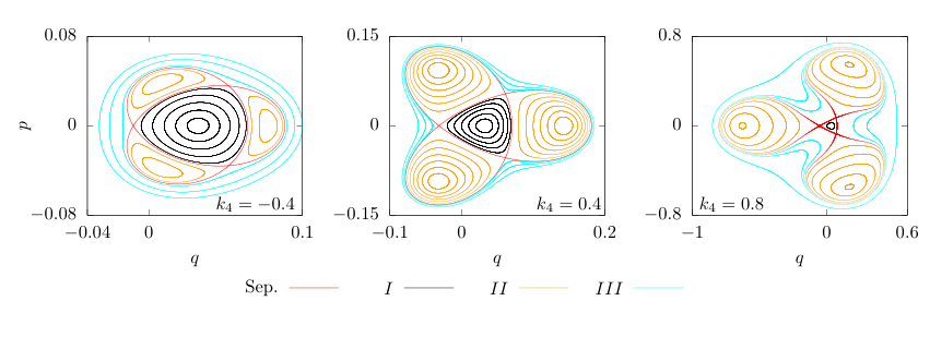
Although the global topology is equivalent for all three cases, the detail is not, implying that the surface variation with time of the resonance islands might be rather different between the three cases considered. This would have an important impact on the trapping and transport phenomena.
The impact of the term on the trapping fraction has been studied by means of numerical simulations that have been performed on a model of type and a second one of type to assess the behavior for different types of time-dependent perturbations. The results are shown in Fig. 14, for the (top) and the (bottom) cases.
For the model, three cases corresponding to different values of have been considered. A strong dependence of the trapping fraction on is clearly visible, with being also a parameter with a strong impact on trapping.
For the model, a mild dependence of the trapping fraction on is observed. However, the two cases corresponding to different values of behave differently as a function of . For the two cases feature equal values of the trapping fraction, whereas for differences are visible.
It is worth stressing that even for this more complex model, which shows peculiar features, the trapping and transport processes have been designed using the criteria presented and discussed for the simpler models. This is an indication that the theory, developed for the basic models can also be used to interpret more general cases.
6 Conclusions
In this paper, a class of dynamical systems has been considered, in which nonlinear effects are combined with a time-dependent external exciter. This class of systems has been studied both in terms of Hamiltonian as well as using a nonlinear symplectic map. The goals of our analyses were to assess the possibility of deriving effective scaling laws for the efficiency of resonance trapping for adiabatically perturbed symplectic maps using the analytical results of adiabatic theory for Hamiltonian systems, and to identify the application of this class of systems to perform trapping and transport in phase space. Both aspects have been successfully carried out.
The comparison between Hamiltonian and symplectic map systems has been considered in detail. It has been shown that the adiabatic theory for Hamiltonian systems provides the appropriate framework to describe the trapping and transport phenomena for nonlinear symplectic maps, too. We have shown that adiabatic trapping into stable resonance islands while modulating a periodic, time-dependent perturbation, is an efficient mechanism for phase-space particle transport. A protocol to vary the two system parameters, namely, the strength and frequency of the time-dependent perturbation, has been proposed, which successfully addresses this aspect. The dynamic mechanisms occurring during the separatrix change in phase space have been understood for different models, highlighting the phase-space structure, and comparing the results of the numerical simulations with the theoretical predictions. Several scaling laws have been studied, and extensive simulations have been performed to probe the dependence of trapping and transport features as a function of the systems’ parameters.
The extension of these results to realistic models, as required by physical applications, implies considering multidimensional systems, for which the theory still needs to be fully developed. Nonetheless, the results presented in this paper open a road-map for a feasibility study to apply the resonance trapping induced by an external periodic perturbation in the field of particle accelerators, as a possible improvement of the novel beam manipulations that have been developed to trap beams of charged particles in a circular accelerator.
Acknowledgments
We are indebted to Prof. A. Neishtadt for several discussions and useful suggestions. One of the authors (A.B.) would like to thank the CERN Beams Department for the hospitality during the preparation of this work.
Appendix A Perturbative analysis of an Hamiltonian system with a time-dependent exciter
It is convenient to introduce the linear action-angle variables using , , and the Hamiltonian (4) reads
| (30) |
We denote by the action-angle variables of the unperturbed Hamiltonian, i.e. for , and turns out to be the adiabatic invariant of the system when no resonance condition is fulfilled.
To study the adiabatic trapping, we compute the parametric dependence of from the nonlinear terms using a perturbative approach [40]. We apply the Lie transformation using a generating function
| (31) |
and we obtain a Normal Form Hamiltonian
| (32) |
The perturbative equation for reads
| (33) |
and it can be integrated, yielding
| (34) |
At first order, the change of variables reads
| (35) | ||||
and the coefficient of the Normal Form Hamiltonian is the average value
| (36) |
The strength of the th-order resonance, , is given by the th Fourier coefficient of , i.e.
| (37) |
so that to study the third-order resonance () with a linear forcing (), we can truncate the expansion at , because higher-order terms in will not have a projection on the Fourier coefficient of .
The perturbation term is proportional to and setting and expanding up to , we obtain
| (38) | ||||
The coefficient of the term reads
| (39) |
and its Fourier coefficient of order 3 is
| (40) |
Performing analogous computations for the case and , the term can be written in the form
| (41) | ||||
and the Fourier coefficient of is given by
| (42) |
By comparing the coefficient with the corresponding coefficient , one determines the different scale of the perturbation strength in the two cases, namely
| (43) |
Finally, we observe that the expansion of starts at , whereas the one of starts at . In general, given a perturbation, the lowest-order term is given by . This means that resonances with are excited by higher-order perturbation terms, so that the expected relevance for applications is considerably reduced.
We remark, that the Hamiltonian (30) can be analyzed using a different approach. In the new variables one obtains an approximate Hamiltonian of the form
| (44) |
and we can introduce the slow phase via a time-dependent generating function . Setting as the distance from the resonance, we have
| (45) |
and defining the parameters
| (46) |
one obtains by rescaling the Hamiltonian
| (47) |
The dynamics generated by this Hamiltonian can be studied, for what concerns trapping via separatrix crossing, with the methods exposed in [23, 24]. Its phase space, in fact, features, depending on and , an hyperbolic point at the crossing of separatrices, which enclose an inner and an outer region.
Appendix B Analysis of the minimum trapping action
From the observations reported in the main body of the article, for any value of or the phase-space islands appear at some amplitude, which determines the smallest radius for which particles are trapped into the islands. A simplified approach to determine an estimate for the minimum action starts from the Hamiltonian
| (48) |
that corresponds to a forced nonlinear oscillator with a resonance condition
| (49) |
that defines the resonant action (when it is real). Note that it is always possible to introduce the angle and the re-scaling of the action , so that the Hamiltonian reads
| (50) |
The resonant phase can be introduced by using the generating function
| (51) |
and one obtains the pendulum-like system
| (52) |
To study the nonlinear resonance crossing, we assume
| (53) |
so that the resonance amplitude in phase space is given by
| (54) |
We can further reduce the Hamiltonian to that of a forced pendulum by using the generating function
| (55) |
and the new Hamiltonian has the form
| (56) |
where () and . The condition for the existence of fixed points is
| (57) |
The first equation provides the resonance position in phase space, whereas the second one provides a condition on the existence of the resonance since we obtain
| (58) |
and . We observe that for (adiabatic parameter) we have the existence of the resonance for small values of the actions . However, for fixed ratio we obtain a condition for the resonance as
| (59) |
where is a suitable constant, which means the existence of a minimal trapping action that scales as
| (60) |
and, e.g. for then .
References
- [1] V. I. Arnol’d, V. Kozlov, and A. Neishtadt. Mathematical Aspects of Classical and Celestial Mechanics. Springer, 2006.
- [2] B. V. Chirikov and V. V. Vecheslavov. Adiabatic Invariance and Separatrix: Single Separatrix Crossing. Journal of Experimental and Theoretical Physics, 90-3:562, 2000.
- [3] A. Neishtadt. Passage through a separatrix in a resonance problem with a slowly-varying parameter. J. Appl. Math. Mech., 39:594, 1976.
- [4] A. Neishtadt. Change of an adiabatic invariant at a separatrix. Sov. J. Plasma Phys., 12:568, 1986.
- [5] A. Neishtadt. Scattering by resonances. Celestial Mechanics and Dynamical Astronomy, 65:1, 1997.
- [6] D. Vainchtein and I. Mezić. Capture into Resonance: A Method for Efficient Control. Phys. Rev. Lett., 93:084301, 2004.
- [7] A. Neishtadt. Capture into resonance and scattering on resonances in two-frequency systems. Proceedings of the Steklov Institute of Mathematics, 250:183, 2005.
- [8] A. Bazzani, F. Brini, and G. Turchetti. Diffusion of the Adiabatic Invariant for Modulated Symplectic Maps. AIP Conf. Proc. 395, 129, 1997.
- [9] V. I. Arnol’d. On the behavior of adiabatic invariants under a slow periodic change of the Hamiltonian function. Doklady, 142:758, 1962.
- [10] V. I. Arnol’d. Conditions of the applicability and an estimate of the mistake of the averaging method for systems, which goes through the resonances during the evolution process. Doklady, 161:9, 1965.
- [11] A. Neishtadt. Jumps in the adiabatic invariant on crossing the separatrix and the origin of the 3:1 Kirkwood gap. Sov. Phys. Dokl., 32:571, 1987.
- [12] S. Sridhart and J. Touma. Adiabatic evolution and capture into resonance: vertical heating of a growing stellar disc. Mon. Not. R Astron. Soc., 279:1263, 1996.
- [13] V. Chirikov. Particle confinement and adiabatic invariance. Proc. Royal Soc. London A, 413:145, 1987.
- [14] D.F. Escande. Contributions of plasma physics to chaos and nonlinear dynamics. Plasma Physics and Controlled Fusion, 58-11, 2016.
- [15] R. Cappi and M. Giovannozzi. Novel Method for Multiturn Extraction: Trapping Charged Particles in Islands of Phase Space. Phys. Rev. Lett., 88:104801, 2002.
- [16] R. Cappi and M. Giovannozzi. Multiturn extraction and injection by means of adiabatic capture in stable islands of phase space. Phys. Rev. ST Accel. Beams, 7:024001, 2004.
- [17] A. Huschauer, A. Blas, J. Borburgh, S. Damjanovic, S. Gilardoni, M. Giovannozzi, M. Hourican, K. Kahle, G. Le Godec, O. Michels, G. Sterbini, and C. Hernalsteens. Transverse beam splitting made operational: Key features of the multiturn extraction at the cern proton synchrotron. Phys. Rev. Accel. Beams, 20:061001, Jun 2017.
- [18] S. Gilardoni, M. Giovannozzi, M. Martini, E. Métral, P. Scaramuzzi, R. Steerenberg, and A.-S. Müller. Experimental evidence of adiabatic splitting of charged particle beams using stable islands of transverse phase space. Phys. Rev. ST Accel. Beams, 9:104001, 2006.
- [19] A. Franchi, S. Gilardoni, and M. Giovannozzi. Progresses in the studies of adiabatic splitting of charged particle beams by crossing nonlinear resonances. Phys. Rev. ST Accel. Beams, 12:014001, 2009.
- [20] A. Neishtadt, A. A. Vasiliev, and A. Itin. Captures into resonance and scattering on resonance in dynamics of a charged relativistic particle in magnetic field and electrostatic wave. Physica D, 141:281, 2000.
- [21] A. N. Vasil’ev and M. A. Guzev. Particle capture by a slowly varying potential. Theor. Math. Phys., 68:907, 1986.
- [22] A Bazzani, C Frye, M Giovannozzi, and C Hernalsteens. Analysis of adiabatic trapping for quasi-integrable area-preserving maps. Phys. Rev. E, 89(CERN-ACC-2014-0042):042915. 22 p, Apr 2014.
- [23] A. I. Neishtadt. Passage through a separatrix in a resonance problem with a slowly-varying parameter. Journal of Applied Mathematics and Mechanics, 39(4):594 — 605, 1975.
- [24] A. I. Neishtadt, A. A. Vasil’ev, and A. V. Artem’ev. Capture into resonance and escape from it in a forced nonlinear pendulum. Regular and Chaotic Dynamics, 18(6):686–696, Nov 2013.
- [25] R. Cappi and M. Giovannozzi. Novel method for multiturn extraction: Trapping charged particles in islands of phase space. Physical Review Letters, 88:104801, Feb 2002.
- [26] J. Borburgh, S. Damjanovic, S. Gilardoni, M. Giovannozzi, C. Hernalsteens, M. Hourican, A. Huschauer, K. Kahle, G. Le Godec, O. Michels, and G. Sterbini. First implementation of transversely split proton beams in the CERN Proton Synchrotron for the fixed-target physics programme. EPL, 113(3):34001. 6 p, 2016.
- [27] V. I. Arnold and A Avez. Problèmes Ergodiques de la Mécanique Classique. Gauthier-Villars, Paris, 1967.
- [28] M. Hénon. Numerical study of quadratic area-preserving mappings. Q. Appl. Math., 27:291, 1969.
- [29] Armando Bazzani, G Servizi, Ezio Todesco, and G Turchetti. A normal form approach to the theory of nonlinear betatronic motion. CERN Yellow Reports: Monographs. CERN, Geneva, 1994.
- [30] R. Tomás. Normal form of particle motion under the influence of an ac dipole. Phys. Rev. ST Accel. Beams, 5:054001, May 2002.
- [31] R. Tomás, M. Bai, R. Calaga, W. Fischer, A. Franchi, and G. Rumolo. Measurement of global and local resonance terms. Phys. Rev. ST Accel. Beams, 8:024001, Feb 2005.
- [32] R. Tomás. Adiabaticity of the ramping process of an ac dipole. Phys. Rev. ST Accel. Beams, 8:024401, Feb 2005.
- [33] R. Miyamoto, S. E. Kopp, A. Jansson, and M. J. Syphers. Parametrization of the driven betatron oscillation. Phys. Rev. ST Accel. Beams, 11:084002, Aug 2008.
- [34] S. White, E. Maclean, and R. Tomás. Direct amplitude detuning measurement with ac dipole. Phys. Rev. ST Accel. Beams, 16:071002, Jul 2013.
- [35] N. Biancacci and R. Tomás. Using ac dipoles to localize sources of beam coupling impedance. Phys. Rev. Accel. Beams, 19:054001, May 2016.
- [36] R. Bartolini, M. Giovannozzi, A. Bazzani, W. Scandale, and E. Todesco. Algorithms for a precise determination of the betatron tune. In S. Myers, editor, EPAC 96, pages 1329–1334. IOP, 1996.
- [37] J. Laskar. Introduction to frequency map analysis. In Carles Simó, editor, Hamiltonian Systems with Three or More Degrees of Freedom, pages 134 — 150, Dordrecht, 1999. Springer, Springer.
- [38] Maxim, https://math.stackexchange.com/users/491644/maxim. Asymptotic expansion of as . Mathematics Stack Exchange, https://math.stackexchange.com/questions/4167778/asymptotic-expansion-of-int-02-pi-mathrmd-theta-sqrtk2-cos2-theta#comment8640217_4167778, 2021. Accessed: 2021-06-10.
- [39] J. Candy and W. Rozmus. A symplectic integration algorithm for separable hamiltonian functions. Journal of Computational Physics, 92(1):230 — 256, 1991.
- [40] Giorgio Turchetti. Dinamica classica dei sistemi fisici. Zanichelli, Bologna, 1998.