An Online, Dynamic Amplitude-Correcting Gradient Estimation Technique to Align X-ray Focusing Optics

The definition below is assembled similarly to that seen in Definition 1, but coordinates all sampling according to a uniformly-discretized time series. A example diagram is provided in Figure 2. If the sampling distance $\delta>0$ remains uniform, it is assumed that the time required to visit each point within the sequence is uniform. While this isn’t a necessary limitation in practice, this assumption simplifies the analysis provded in A.

If we use the following short-hand for the standard central-differencing stencil (in spatial coordinates), directional derivatives can be written

Our convention of selecting antipodal points in sequence allows us to utilize these directional derivative stencils directly. Since each observation of $G({\bf x},t)$ results in an independent noise term $\varsigma$, combining like-terms results in

Rosenbrock’s Valley Rosenbrock is a polynomial on $\mathbb{R}^{2}$ defined as

This polynomial has a global minimum value of $f(1,1)=0$, and is locally convex around that point. However, the downward slope along the minimal ridge is quite low in the parabolic valley. It is this feature that made Rosenbrock’s Valley a popular benchmark, since many steepest descent algorithms tend to reach the ridge quite quickly, but struggle to reach the optimal answer due to the oscillations spurred from the large values of $|\nabla f(x,y)|$ for $(x,y)$ not precisely on the ridge path. In the interest of clarity, we will refer to these as spatial oscillations.

The classic benchmark nonlinear programming problem is typically presented as

We complicate matters by including the amplitude function $T(t)$ such that

where

Again, for the sake of clarity, we shall refer to oscillations caused by a dynamic amplitudes like (5) as temporal oscillations.

In our first experiment, we attempt to solve our temporally oscillating problem (4) with the standard gradient descent method (Algorithm 1.) We initialize at ${\bf x}_{0}=(-1.2,1)$, fix $\alpha_{i}=\delta=1/500$, $\beta=0$, enforce a step-size maximum $||{\bf x}_{i+1}-{\bf x}_{i}||\leq 1/4$, and a maximum iteration count of $i_{\text{max}}=1200$. The gradient is computed by a uniform sampling of $N=15$ antipodal pairs. In Figure 3, we see that the gradient estimates are erroneous far beyond what can be tolerated by the standard algorithm. The figure only depicts steps up to $i_{200}$, since the full path eventually diverges. Increasing the momentum value $\beta$ has no appreciable impact on this outcome.

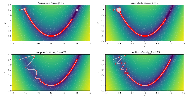
In the second experiment, we seek to demonstrate that our amplitude correcting gradient estimate is effective in overcoming the temporal oscillations imposed by (5). We accomplish this by comparing the performance of Algorithm 2, which utilizes the dynamic amplitude correction, on the temporally-oscillating problem (4) to the performance of classic gradient descent method in Algorithm 1 on the non temporally-oscillating problem in (3). For each execution we initialize at ${\bf x}_{0}=(-1.2,1)$, selecting $\alpha_{i}=\delta=1/500$, $\beta=0$, enforce a step-size maximum $||{\bf x}_{i+1}-{\bf x}_{i}||\leq 1/4$, and a maximum iteration count of $i_{\text{max}}=1200$. The gradient is computed by a uniform sampling of $N=15$ antipodal pairs. In the temporally oscillating problem, we prescribe a time-step of $h=1/16$. We provide comparisons with, and without momentum in Figure 4.

In the first row of Figure 4 we see that without momentum ($\beta=0$) neither implementation manages to overcome the spatial oscillations. By iteration count $i_{\text{max}}=1200$, both executions seem to terminate in roughly the same position. In the second row, we see that when momentum is included, both methods overcome the spatial oscillations and reach the global minimum position. When considering the apparent qualitative similarity between these outcomes, in conjunction with the failure demonstrated in Figure 3, we posit that the amplitude corrections are effective in mitigating the temporal oscillations imposed on (4).

The following theorem provides conditions sufficient for the convergence of the standard differencing gradient in SGD (Algorithm 1), as well as an error estimate. Proof can be found in Nguyen2019.

The following result presents convergence of the stochastic gradient descent method in terms of the error seen in the gradient estimates of the cost function.

We now look to numerically verify the convergence of Algorithm 2 on the problem:

where the cost function

with $\mathbf{\Sigma}$ given by

We proceed by first demonstrating that an a priori accuracy of the SGD algorithm can be written in terms of the asymptotic error of our gradient estimate developed in Theorem 2.2. This allows us to formalize a parameterization of the error developed in Algorithm 2 as a function of $\delta,h,\sigma,$ and $N,$ and to test the error rates. As before, the additive noise term $\varsigma(t)$ is i.i.d. and $\mathcal{N}(0,\sigma)$. The asymptotic error of the dynamic amplitude-correcting gradient estimates of $G$ are given, in expectation, in Corollary 2. Proof of the following comes directly from Theorems 2.1, 2.2, and Young’s inequality.

These error estimates are verified in a series of Monte Carlo studies. For each parametrization, we repeat and store the results from 30 executions of Algorithm 2, storing the results in

In the first experiment, we fix $\delta$, $\sigma$, and $N$ such that their contributions to the error in (8) are several orders of magnitude below our choices for $h$. We further assume that $L\approx||\mathbf{\Sigma}||_{2}=2+\sqrt{2}/2,$ which gives for $h$ sufficiently small, that our critical algorithm step $\tau$ is $\mathcal{O}(h^{-2}).$ Selecting a fixed step-size $\alpha_{i}=\delta$, with a fixed stopping point, trivially satisfies the convergence requirements of Theorem 3.1. In addition, given our estimate of $\tau$, and the minimum travel distance required, selecting $N=5$, and $\delta=$1/100, we find a choice of $i_{\text{max}}=500$ to be appropriate. The results of this test confirm the a priori rate estimate of $\mathcal{O}(h^{2})$, and are presented in terms of the average result over the 30 simulations in Table 1.

We proceed similarly in the second experiment. We fix $h=1/1024$, $N=10$, and $\delta=1/100$, varying $\sigma$. Noting that smallest choice for $\sigma=1/2560$, we again estimate the critical time-step as $\tau=$ 500. The optimal rates are observed and presented in Table 2.

For the third, we fix $N$=256, $\sigma$ = 1/2048, and $h$ = 1/2048, varying $\delta.$ We maintain our choice of $i_{\text{max}}$ = 500, presenting the results in Table 3. We see rates comparable to the $\mathcal{O}(\delta^{4})$ rate.

In our final experiment, we test the linear convergence rate of the sampling count parameter $N.$ Fixing $h$ = 1/1024, $\delta$ = 1/100, and $\sigma$ = 0.64, varying $N$. We select $i_{\text{max}}=500$. In Table 4 we see convergence at a rate slightly better than the expected $\mathcal{O}(N^{-1})$ rate.

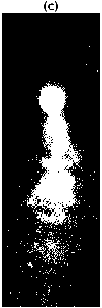
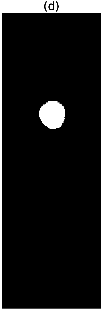
Let $\Omega_{max}\subset\mathbb{R}^{4}$ denote the travel limits for the four stepper motors that determine the orientation of the CRL. For a given orientation ${\bf x}=(x,y,r_{x},r_{y})\in\Omega$, let the resulting image deposited on the detector panel be denoted as $I({\bf x}),$ or simply $I$ when convenient; see Figure 1. Further, we describe position of a given pixel by its indices $I_{i,j}.$ Example detector images are shown in Figures 5(a) and (b).

Let $\xi(I)$, $\mu(I)$ and $\sigma(I)$ denote the median, mean, and standard deviation, respectively, of the pixel values of the image $I$. We then constrain $I$ to a selected region of interest (ROI) defined as

where $M>0$ is a user-selected threshold parameter. In practice, we found $M=2$ to be a good choice. Figure 5 (c) and (d) highlight the corresponding ROIs, $\hat{I}_{M}.$

In the synchrotron experiments performed at the Advanced Photon Source in Breckling2021, a set of coordinates found by manual alignment were defined as the ground-truth to provide the “well-aligned” position of the CRL. We denote that position as ${\bf x}^{*}=(x^{*},y^{*},r_{x}^{*},r_{y}^{*})$. This ground truth served two purposes. First, we were then able to define a feature scaling such that our metric of X-ray transmission, in terms of CRL orientation,

had a maximal value of 1. Second, the ground-truth position allowed us to establish a four-dimensional rectangular region $\hat{\Omega}\subset\Omega_{max}$ around the best point that contained the support of $f$ above the noise floor. With this ground-truth and 4D window, we then collected several raster scans of $f(\hat{\Omega};M=2)$. We make use of a full four-dimensional scan, and two high-resolution, independent, 2-dimensional raster scans of $\hat{\Omega}$.

Assuming a steady beam amplitude, it follows from the model developed by Simons et al. that an idealized transmission function $f:\mathbb{R}^{4}\rightarrow\mathbb{R}^{+}$ is given by a 4-variate Gaussian distribution simons17. We generalize that model as

where $a,b\in\mathbb{R}$, the matrix $\mathbf{A}\in\mathbb{R}^{4\times 4}$ is symmetric, and $\hat{{\bf x}}\in\mathbb{R}^{4}$ is the position associated with optimal lateral alignment. Fitting the four-dimensional raster scan data $f(\hat{\Omega};M=2)$ to Simons’ model (10) gives the idealized X-ray transmission $f_{\text{Simons}}^{*}({\bf x})$. We present two, two-dimensional slice views of $f_{\text{Simons}}^{*}({\bf x})$ in Figure 7.

To model the noise functions that are characteristic to the XFEL light sources, we include additive measurement noise as $\varsigma_{\Omega}(t)$. Let $\text{diam}(\hat{\Omega})$ denote the maximal diameter of the set $\hat{\Omega}$. We collected a sampling $\mathcal{S}=\{{\bf x}_{i}\}_{i=1}^{500}$ such that for every orientation ${\bf x}_{i}$, $||{\bf x}_{i}-{\bf x}^{*}||>\text{diam}(\hat{\Omega})$. We found that $\sigma(f(\mathcal{S};M=2))\approx 4.5\times 10^{-3}.$ We then model the time-series of additive noise $\varsigma_{\Omega}(t)$ as i.i.d. and $\mathcal{N}(0,4.5\times 10^{-3})$.

We additionally consider fluctuations that occur because of pointing jitter (from the SASE generation scheme) kang2017hard. We assume the position and direction of the beam may randomly fluctuate as a function of the beam’s divergence profile, which was estimated at the APS to be 6.5$\times 10^{-3}$ Radians. We account for jitter in our model as random perturbations of the orientation vector ${\bf x}$ in the $r_{x}$ and $r_{y}$ directions. Further, we expect that the beam will jitter randomly within 10% of the beam-divergence. In doing so, we define

where $\theta_{x}$ and $\theta_{y}$ are respectively i.i.d and $\mathcal{N}(0,6.5\times 10^{-4})$.

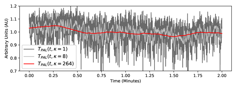
We lastly introduce the fluctuating intensity of the beam over time. To this end, we utilize the measured shot-to-shot intensity values recorded at the PAL-XFEL facility, which was recorded using a quadrant beam position monitor (QBPM) at 30 Hz DresselhausMarais2020. We feature-scale the raw pulse-to-pulse time-series data by normalizing the full signal against the mean recorded value. This scaled signal is written as $T_{\text{PAL}}(t,\kappa)$ where $\kappa$ determines the number of pulses averaged during a data collection event. In Figure 8 we show $T_{\text{PAL}}(t,1)$ in dark gray, $T_{\text{PAL}}(t,8)$ in light gray, and $T_{\text{PAL}}(t,264)$ in red. The mollified signals at $\kappa=8$ and $\kappa=264$ respectively represent the average beam intensity over a sampling interval, and the amount of time required to collect all samples necessary to compute the amplitude-correcting gradient.

Our full cost function model is hence written and evaluated as

We now endeavor to study the performance of Algorithm 2 on our model of the CRL alignment problem

Our goal is to identify a range of nominal parameter choices for Algorithm 2 that can be implemented as a starting point at an XFEL facility.

We begin by noting that when sampling (11) to estimate $\nabla f_{\text{Simons}}^{*}({\bf x})$ as per Definition 2, we consider $N=8$ quasi-uniformly distributed antipodal pairs in our differencing stencil. We select our effective integration time interval for the camera to be $h_{\text{cam}}=8/30$ seconds, and establish the full time interval required to complete the scheme as $\mathcal{T}_{h,N}:=[t_{0},(4N+1)h+t_{0}].$ Further, we make use of the estimate

where $t_{0}$ is the moment we began estimating the gradient.

For each execution of Algorithm 2 that follows, the stopping condition is established to be a maximal iteration count $i_{\text{max}}.$ No other stopping conditions are considered. Additionally, we conceptualize our initial gradient sphere radius $\alpha_{0}$ as some multiple $Cr,$ where $r=||{\bf x}_{0}-\hat{{\bf x}}||,$ though we don’t expect users to know what $r$ is a priori. At each step $i$, the gradient sampling radius $\alpha_{0}$ is scaled by a cooling factor such that

where $\gamma>0$ and fixed. Further, we enforce a maximum step size $||{\bf x}_{i}-{\bf x}_{i-1}||\leq\delta_{i}=\alpha_{i}.$ Given that the true distance $r$ is unknown upon initialization, the executions that follow are intended to identify a performance relationship between $\alpha_{0}$ with respect to $r$, $\gamma$, and the stopping condition.

We demonstrate a single execution of Algorithm 2 with an initial position ${\bf x}_{0}$ selected randomly a distance of $r=0.4$ from $\hat{{\bf x}}.$ We note that this Euclidean distance is significantly further away from $\hat{{\bf x}}$ than the positions selected during the manually-tuned rough alignments completed during data collections at the more stable synchrotron source at APS Breckling2021. We fix $\gamma=0.3$, select $\alpha_{0}$ according to the distance scalar $C=3.0$, assign a momentum term $\beta=0.15,$ and set the stopping condition to $i_{\text{max}}=100$ iterations. In addition to the time required to collect the image data from the camera sensor $h_{\text{cam}}$, we need to include an estimate of the time required to move the four stepper motors, and process the data. We assume $h_{\text{move}}=5/30s$. Given the full time interval time interval $h_{\text{total}}=h_{\text{cam}}+h_{\text{move}}=13/30s$, the total execution time assumed necessary to reach 100 iterations is

or 23.8 minutes. A figure depicting the particular route taken is presented in the 2D projections shown in Figure 9.

Next, we present the result of three Monte Carlo experiments. We maintain the parameter choices established in the execution above, varying only the stopping condition $i_{\text{max}}=50,100,$ and $200$. Each Monte Carlo executes Algorithm 2 to completion 100 times, varying the initial position randomly on $\partial\mathcal{B}_{r}({\bf x}_{0})$ where $r=0.4.$ The results depicted in Figure 10 demonstrate the expected convergence behavior for those well-selected parameters.

What remains to be assessed is performance as a function of the user’s choice of step size, and cooling parameter. We consider two values for the cooling parameter $\gamma$, five initial step-size scales $C$, and six stopping conditions $i_{\text{max}}.$ For each particular set of parameters, Algorithm 2 is executed 100 times, where the starting position ${\bf x}_{0}$ is again sampled randomly from $\partial\mathcal{B}_{r}(\hat{{\bf x}})$. These regions demonstrate a collection of parameters that tend to reliably converge under an hour ($i_{\text{max}}<200$ iterations.)

While additional parameters remain to be thoroughly studied, namely the momentum term $\beta,$ we found that choices of $\beta>0.15$ tended to perform poorly over longer periods of computation time. In particular, when $i_{\text{max}}>50$ we saw no apparent improvement to performance. Given that the settings identified above demonstrate convergence that tends to improve with additional computation, an attractive behavior for an unsupervised optimization method, we advise being conservative with $\beta.$ We additionally note that our choice to equate the maximal step-size with the gradient diameter was born out of observation. Choices of $\alpha_{i}$ substantially larger than $\delta_{i}$ frequently resulted in failure over longer time intervals. Lastly, we observed that selecting $\gamma$ too large tended to collapse $\alpha_{i}$ too quickly, which was also detrimental to long-time performance. Conversely, selecting $\gamma$ too small tends to result in slow convergence.

References

- (1) B. Lengeler, C. Schroer, J. TuÈmmler, B. Benner, M. Richwin, A. Snigirev, I. Snigireva, M. Drakopoulos, Imaging by parabolic refractive lenses in the hard x-ray range, J. Synchrotron Radiat. 6(6), 1153 (1999)
- (2) C.G. Schroer, O. Kurapova, J. Patommel, P. Boye, J. Feldkamp, B. Lengeler, M. Burghammer, C. Riekel, L. Vincze, A. van der Hart, et al., Hard X-ray nanoprobe based on refractive x-ray lenses, Appl. Phys. Lett. 87(12), 124103 (2005)
- (3) G.B.M. Vaughan, J.P. Wright, A. Bytchkov, M. Rossat, H. Gleyzolle, I. Snigireva, A. Snigirev, X-ray transfocators: focusing devices based on compound refractive lenses, J. Synchrotron Radiat. 18(2), 125 (2011)
- (4) M. Yabashi, H. Tanaka, The next ten years of X-ray science, Nature Photonics 11(1), 12 (2017)
- (5) P. Emma, R. Akre, J. Arthur, R. Bionta, C. Bostedt, J. Bozek, A. Brachmann, P. Bucksbaum, R. Coffee, F.J. Decker, Y. Ding, D. Dowell, S. Edstrom, A. Fisher, J. Frisch, S. Gilevich, J. Hastings, G. Hays, P. Hering, Z. Huang, R. Iverson, H. Loos, M. Messerschmidt, A. Miahnahri, S. Moeller, H.D. Nuhn, G. Pile, D. Ratner, J. Rzepiela, D. Schultz, T. Smith, P. Stefan, H. Tompkins, J. Turner, J. Welch, W. White, J. Wu, G. Yocky, J. Galayda, First lasing and operation of an ångstrom-wavelength free-electron laser, Nature Photonics 4(9), 641 (2010)
- (6) E. Schneidmiller, M. Yurkov, in Proceedings of the 7th International Particle Accelerator Conference (IPAC 2016), Busan, Korea (2016)
- (7) H. Simons, S.R. Ahl, H.F. Poulsen, C. Detlefs, Simulating and optimizing compound refractive lens-based X-ray microscopes, J. Synchrotron Radiat. 24(2), 392 (2017)
- (8) S. Breckling, B. Kozioziemski, L. Dresselhaus-Marais, P. Chow, A. Gonzalez, H. Simons, A. Williams, M. Howard, An automated approach to the alignment of compound refractive lenses (Draft Under Peer Review), Journal of Synchrotron Radiation (JoSR) (2021)
- (9) M. Belen’kii, J. Barchers, E. Berg, D. Bruns, D. Fung, R. Gallant, C. Kirk, H. Runyeon, V. Rye, J. Voass, in Atmospheric Optics: Models, Measurements, and Target-in-the-Loop Propagation, vol. 6708 (International Society for Optics and Photonics, 2007), vol. 6708, p. 67080I
- (10) A. Arockia Bazil Raj, J. Arputha Vijaya Selvi, S. Raghavan, in 2010 International Conference on Wireless Communication and Sensor Computing (ICWCSC) (2010), pp. 1–5
- (11) M. Li, X. Liu, A. Zhang, X. H., Testing of the stochastic parallel gradient descent algorithm for the alignment of a two-mirror telescope, J. Opt. Technol. 87(5), 276 (2020)
- (12) J. Spall, Introduction to Stochastic Search and Optimization, 1st edn. (Wiley, USA, 2003)
- (13) Y. Nesterov, Lectures on Convex Optimization, 2nd edn. Springer Optimization and Its Applications, 137 (Springer International Publishing : Imprint: Springer, 2018)
- (14) H.H. Rosenbrock, An automatic method for finding the greatest or least value of a function, Comput. J. 3(3), 175 (1960)
- (15) L. Nguyen, P. Nguyen, P. Richtárik, K. Scheinberg, M. Takáč, M. van Dijk, New convergence aspects of stochastic gradient algorithms, J. Mach. Learn. Res. 20 (2019)
- (16) H. Kang, C. Min, H. Heo, C. Kim, H. Yang, G. Kim, I. Nam, S.Y. Baek, H. Choi, G. Mun, B.R. Park, Hard x-ray free-electron laser with femtosecond-scale timing jitter, Nature Photonics 11(11), 708 (2017)
- (17) L.E. Dresselhaus-Cooper. PAL experimental report form (2020)
- (18) R. Vershynin, High-Dimensional Probability: An Introduction with Applications in Data Science. Cambridge Series in Statistical and Probabilistic Mathematics (Cambridge University Press, 2018)
- (19) M. Wainwright, High-Dimensional Statistics: A Non-Asymptotic Viewpoint. Cambridge Series in Statistical and Probabilistic Mathematics (Cambridge University Press, 2019)
Appendix A Accuracy Estimates
Below we have appended error estimates of the amplitude-correcting gradient tool presented in this manuscript. Accuracy is discussed in terms of both spatial and temporal discretizations, as well as the case where Gaussian, i.i.d. noise is present.
Lemma 1 (Error Estimate of a Single Directional-Derivative Stencil on Smooth Functions)
Proof.
We proceed by showing that our differencing stencil reduces to the central difference scheme with additional error sources to consider. Assemble the finite differences, and replace each term with its separated counterparts:
Add and subtract and to the right-hand side. When we combine like terms we see