Enhancement Encoding: A Novel Imbalanced Classification Approach via Encoding the Training Labels
Abstract
Class imbalance, which is also called long-tailed distribution, is a common problem in classification tasks based on machine learning. If it happens, the minority data will be overwhelmed by the majority, which presents quite a challenge for data science. To address the class imbalance problem, researchers have proposed lots of methods: some people make the data set balanced (SMOTE [6]), some others refine the loss function (Focal Loss [33]), and even someone has noticed the value of labels influences class-imbalanced learning (Yang and Xu. Rethinking the value of labels for improving class-imbalanced learning. In NeurIPS 2020 [48]), but no one changes the way to encode the labels of data yet. Nowadays, the most prevailing technique to encode labels is the one-hot encoding due to its nice performance in the general situation. However, it is not a good choice for imbalanced data, because the classifier will treat majority and minority samples equally. In this paper, we innovatively propose the enhancement encoding technique, which is specially designed for the imbalanced classification. The enhancement encoding combines re-weighting and cost-sensitiveness, which can reflect the difference between hard and easy (or minority and majority) classes. To reduce the number of validation samples and the computation cost, we also replace the confusion matrix with a novel soft-confusion matrix which works better with a small validation set. In the experiments, we evaluate the enhancement encoding with three different types of loss. And the results show that enhancement encoding is very effective to improve the performance of the network trained with imbalanced data. Particularly, the performance on minority classes is much better.
1 Introduction
1.1 Class Imbalance Problem
Today, it is widely accepted that the quantity and quality of training data are of great importance for machine learning (ML) [10, 30, 41, 42]. A balanced data set helps a lot for ML, but in quite a few cases, researchers are obliged to process class-imbalanced samples [20, 45]. Class imbalance describes the phenomenon that data of different classes is not uniformly distributed, i.e. instances in some classes are plentiful but others are lacking [17, 5]. When learning from a class-imbalanced training set, the general classifiers try to minimize loss or maximize accuracy on the imbalanced data. It may make the learner overfit the majority classes and underfit the minorities [38, 36]. At inference time, the classifiers will prefer that an unknown instance belongs to the majorities [2, 5], which declines the test accuracy of minority data.
1.2 One-Hot Encoding
One-hot encoding is one of the most prevailing techniques to encode labels or features now [27, 1, 13, 26]. Compared with directly using the index of class as the label, the one-hot encoding technique expresses the label with a vector instead of a number. Suppose there is an instance belonging to class . Its one-hot label can be described as:
where is the total number of classes. Note that the indices of classes start at and end at .
There are some significant advantages of one-hot encoding. Firstly, the label of any one class is “equally” different from all the other ones. More specifically, the Euclidean distance between any pair of different labels is always and the Hemming distance is always . Secondly, one-hot labels work very well with some other fashionable techniques such as Softmax output activation, cross-entropy loss, etc. That’s why one-hot encoding is so popular in classification.
Nevertheless, one-hot encoding is not everything. There are still some problems:
- •
Sparsity: The one-hot labels are too sparse. They are filled with plenty of “0”s and a few “1”s. Too much redundancy of information will eat up memory of the computer.
- •
Unfriendly to imbalanced data: There are always some samples which are more difficult to be classified than others, but one-hot labels can not reflect this difference. This problem is particularly prominent when the data is class-imbalanced.
So, a new encoding technique for labels is demanded.
1.3 Our Work
We have studied how to make full use of one-hot labels’ redundancy to improve the performance of imbalanced classification, and in this paper, we innovatively propose the enhancement encoding technique. In contrast to some other methods for addressing the class imbalance problem (such as oversampling, re-weighting, etc.), it is not compulsory to learn about the distribution of training data for enhancement encoding. That means our method will be very effective when the data is not only imbalanced but also from a stream.
In our algorithm, calculating the confusion matrix on the validation set is a necessary step. Meanwhile, enough validation instances per class are significant for an effective confusion matrix. Unfortunately, it conflicts with the lack of minority data. So, we propose the soft-confusion matrix to replace the confusion matrix. Soft-confusion matrix can work pretty well with a small validation set.
If you want to implement the enhancement encoding in your algorithm, you don’t have to change the structure of your neural network or complicate the backpropagation (BP) too much. Re-encoding labels of the training set is all you need. Thanks to the soft-confusion matrix and fewer validation instances, a little bit of extra computation is just enough.
2 Proposed Approach
2.1 Soft-Confusion Matrix
The confusion matrix is one of the most prevailing metrics in machine learning [47, 50, 23, 46]. If there are classes in the classification, the confusion matrix denoted by is an matrix (). Its element denotes the number of instances belonging to class but classified into class . The greater the diagonal elements, the better the classifier performs.
The confusion matrix is pretty handy in classification, but there are still some shortcomings, such as working poorly when the data is insufficient. To improve the effect and make the most of data, we propose the soft-confusion matrix . is the same size as (), and its elements can be described as:
| (3) |
where denotes the prediction probability that instance belongs to class , is a subset of the data set, which contains all instances belonging to class . That is “” means instance belongs to class . An essential difference between the confusion matrix and the soft-confusion matrix is that the former counts the number of instances and the latter calculates the sum of probability. And obviously, the confusion matrix (without normalization) only contains integers, and the elements of the soft-confusion matrix can be non-integers.
Certainly, the soft-confusion matrix can be calculated by nested loops, but there is a more efficient method via matrix multiplication:
| (4) |
where contains outputs of the classifier and contains one-hot encoded labels. More specifically, the element of is equal to and the element of can be “0” (when instance does not belong to class ) or “1” (when instance belongs to class ). That is:
| (5) |
2.2 The Basic Idea of Enhancement Encoding
As discussed in Section 1.2, one-hot encoding is not a good choice for imbalanced learning. In an imbalanced classification task, identifying a minority instance is much more difficult than identifying a majority one, so it should be better to let the classifier pay more attention to learning from the minority data.
The enhancement encoding is an improved method adapted from the one-hot encoding. The graphical explanation for its basic idea is shown in Figure 1. Because of circumscribed by the output layer’s activation function (such as Softmax and Sigmoid), the elements of the output vector are all less than “1”, greater than “0” and their sum is “1”:
| (9) |
That means points representing outputs are always on the solid line in Figure 1. Meanwhile, enhancement encoding moves the label of minority class from to the location on the dashed line. The process of training can be regarded as making the output and the label closer and closer together. The distance between them is related to the loss. So the new encoding method enhances the part of loss caused by minority samples while training.
The BP algorithm with enhancement encoding
2.3 The Implementation of Enhancement Encoding
In linear block code theory, the generator matrix is usually utilized to encode the information:
| (10) |
where is the message, and is the channel code. Note that and in Equation (10) are row vectors. In this way, the labels can be encoded again to implement the enhancement encoding:
| (11) |
where denotes the one-hot label of instance and denotes the enhancement label. It should be noted that the matrix multiplication in Equation (10) is defined over , but multiplication in Equation (11) is defined over the real number field. An advantage of the label generator matrix is the convenience to express enhancement encoding of multiple instances:
| (12) |
However, how to get the generator matrix is still a question. There are some properties we wish the generator matrix to possess:
- 1.
To re-weight the classes, the diagonal elements should be greater than “1”.
- 2.
To make the labels cost-sensitive, the non-diagonal elements should be less than “0”.
- 3.
To constrain the labels and the classifier outputs in the same hyperplane, as shown in Figure 1, the sum of elements in the same row should be “1”.
That is:
| (13) | |||
| (14) | |||
| (15) |
In consideration of these conditions, we design an algorithm to calculate and update the generator matrix dynamically based on the soft-confusion matrix.
We add some extra steps before a training epoch. Firstly, compute the soft-confusion matrix of the network on the validation set and normalize it. The normalization can be described as follows:
| (16) |
where is the number of instances belonging to class in the validation set. The normalization is to rescale the value into the interval and avoid the trouble of class imbalance in the validation set. Then, calculate the cost matrix :
| (17) |
where denotes the identity matrix. The diagonal of can be negative, which is different from the general cost matrix:
| (18) | |||
| (19) |
Next, update the generator matrix of labels:
| (20) |
where the updating rate and the enhancement rate are two hyper-parameters, is the old generator matrix before updating. When updating , the residual value (i.e. ) is to make the training process more stable. It can be proved easily that the properties described by Expression (13), (14), and (15) are attached to the generator matrix in Equation (20). Lastly, encode the labels of instances in the training set:
| (21) |
where contains the one-hot labels of training instances. The whole BP algorithm can be briefly described as Algorithm 1.
Note that some details are omitted in Algorithm 1, such as adjusting the learning rate dynamically, or regularization, etc. You can add them by yourself if you need to.
The mathematical derivation of enhancement encoding, which proves its effectiveness, is shown in the Appendices.
3 Experiments
In this section, we do some experiments to evaluate the performance of enhancement encoding and report the results in the end.
3.1 Experimental Setup
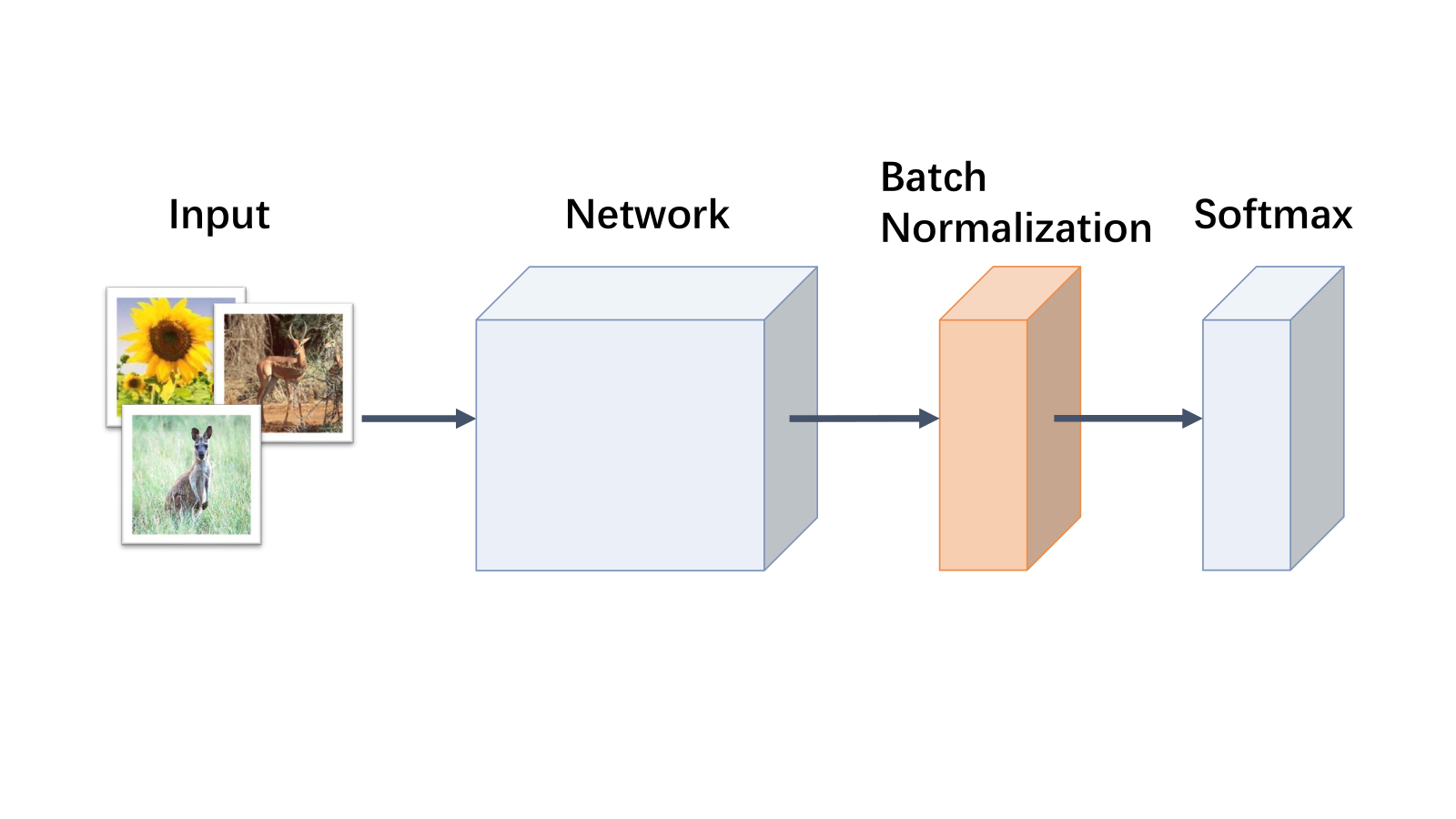
In every experiment, we add a Batch Normalization layer [24] before the output activation function (i.e. Softmax), as shown in Figure 2. The Batch Normalization layer is very helpful to improve the performance of the enhancement encoding. When it is applied, the enhancement rate can be set as a higher value.
MNIST: MNIST [32] is a fairly basic standard data set, which is usually chosen to be the start for learning computer vision. It contains 7,000 handwriting digit images, 6,000 of which are for training and the rest are for tests. The original data set is balanced. To evaluate our algorithm, we manually unbalance the data in two ways: “10% of even classes” and “long-tailed distribution” (see the Appendices). For the first way (10% of even classes), we refer to the data distribution created by Khan et al. [28]. We choose LeNet-5 [32] as the backbone net and make some alterations. We utilize ReLU [15] as the hidden layers’ activation function, utilize Softmax as the output activation function, and replace the original Gaussian connection layer with a fully connected layer.
CIFAR-10-LT: The standard CIFAR-10 [29] is a balanced data set with 10 classes in total. There are 5,000 images for training and 1,000 images for tests per class. We choose its long-tailed version (CIFAR-10-LT) [9] with the imbalance factor of 100 to evaluate our approach. The imbalance factor [9] describes the imbalance degree of the data set. It can be computed by , where denotes the number of instances belonging to class . We randomly select 5 instances per class as the validation set. We choose the ResNet-32 [21] as the backbone net.
Caltech 101: Caltech 101 [14] is an originally imbalanced data set. It contains 8,677 images belonging to 101 classes (exclude the class named “BACKGROUND_Google”). There are about 30800 images per class and the imbalance factor of Caltech 101 is 25.81 (). We randomly split the data set into three parts: a validation set containing 5 images per class, a test set containing 20 images per class, and a training set containing the rest of the data. The resolution of these images is roughly 300200 and we resize them to 224224. The backbone net is ResNet-34.
We compare the performances of enhancement encoding and one-hot encoding in three different situations (cross-entropy loss, mean square error, and focal loss [33]). Focal loss of instance can be expressed as:
| (22) |
where denotes the class weight and denotes the focusing parameter. Because the enhancement labels re-weight the instances of different classes, we set all class weights () as “”.
As mentioned in (13) and (14), the enhancement encoding technique attaches both re-weighting and cost-sensitiveness to the training process. So we also evaluate the incomplete enhancement labels by setting the non-diagonal elements of generation matrix (see Section 2.3) as “0” (marked with “re-weighting”) or setting the diagonal elements as “1” (marked with “cost-sensitiveness”).
| Imbalance Settings | Losses | Baseline (One- Hot Encoding) | Re- Weighting | Cost- Sensitiveness | Enhancement Encoding |
| 10% of Even Classes | MSE | 97.820.03 | 97.92 | 97.89 | 97.990.06 |
| CE | 97.750.04 | 97.85 | 97.91 | 98.000.03 | |
| FL (, ) | 98.060.04 | 98.21 | 98.32 | 98.540.13 | |
| Long-Taile Distribution | MSE | 92.120.56 | 92.56 | 92.61 | 92.780.26 |
| CE | 89.140.13 | 90.95 | 90.65 | 91.430.27 | |
| FL (, ) | 91.560.32 | 91.80 | 91.87 | 93.340.61 |
3.2 Results
| Losses | Methods | Top-1 Accuracy | Minority Accuracy |
| MSE | Baseline (One-Hot Encoding) | 67.150.48 | 49.841.01 |
| Re-Weighting | 67.20 | 50.62 | |
| Cost-Sensitiveness | 67.39 | 50.22 | |
| Enhancement Encoding | 67.890.58 | 51.591.17 | |
| CE | Baseline (One-Hot Encoding) | 65.230.75 | 47.341.56 |
| Re-Weighting | 69.55 | 52.38 | |
| Cost-Sensitiveness | 65.98 | 49.48 | |
| Enhancement Encoding | 69.890.89 | 55.751.73 | |
| FL ( ) | Baseline (One-Hot Encoding) | 67.330.35 | 50.340.78 |
| Re-Weighting | 68.10 | 51.54 | |
| Cost-Sensitiveness | 69.49 | 55.18 | |
| Enhancement Encoding | 69.940.79 | 56.381.24 |
We define the test minority accuracy as the top-1 accuracy evaluated on test instances belonging to minority classes. We regard the minority classes as the classes with the fewest instances in the training set.
For MNIST, we report the top-1 accuracy in Table 1. For CIFA-10-LT, we report the top-1 accuracy and the minority accuracy () in Table 2. And for Caltech 101, top-1 accuracy, top-5 accuracy, and minority accuracy () are shown in Table 3. Obviously, with any one of the three losses, the enhancement encoding always performs better than the one-hot encoding. Particularly, the minority accuracy of enhancement encoding is much higher in all experiments. As shown by the soft-confusion matrices in Figure 3, our method may decline the performance on some majority classes (class 0 and class 1) a little bit, but it improves the performance on minority classes (class 5-9) a lot. In Figure 4, we show the t-SNE visualization [44] of the network’s outputs. It can be found that enhancement encoding makes samples with the same prediction result more concentrated. We run the programs of baseline and enhancement encoding 5 times per situation and report the error bars (MeanSD) in Table 1, Table 2, and Table 3.
Ablation Studies: We evaluate the two incomplete enhancement encoding methods (re-weighting and cost-sensitive) and show the results in Table 1, Table 2, and Table 3. It can be observed that the two types of encoding also perform better than the baseline in most situations. Note the four elements located at the bottom left corner of the normalized soft-confusion matrices (, , , and ) in Figure 3, the cost-sensitiveness is lower, overall. It illustrates that the cost-sensitiveness part of our method is very helpful to mitigate the adverse impact that the majority data overwhelms the minority.


Encoding


| Losses | Methods | Top-1 Accuracy | Top-5 Accuracy | Minority Accuracy |
| MSE | Baseline (One-Hot Encoding) | 54.660.48 | 73.550.37 | 37.320.33 |
| Re-Weighting | 57.03 | 75.05 | 41.10 | |
| Cost-Sensitiveness | 54.75 | 73.22 | 38.60 | |
| Enhancement Encoding | 57.160.87 | 75.820.86 | 41.281.22 | |
| CE | Baseline (One-Hot Encoding) | 58.300.93 | 77.451.56 | 43.140.81 |
| Re-Weighting | 60.50 | 80.15 | 46.90 | |
| Cost-Sensitiveness | 58.81 | 78.42 | 42.70 | |
| Enhancement Encoding | 61.481.07 | 79.500.41 | 47.541.69 | |
| FL ( ) | Baseline (One-Hot Encoding) | 57.281.38 | 77.460.52 | 42.341.61 |
| Re-Weighting | 58.17 | 76.44 | 42.70 | |
| Cost-Sensitiveness | 59.85 | 78.86 | 46.10 | |
| Enhancement Encoding | 60.271.11 | 78.800.88 | 46.821.43 |
4 Related Work
Researches on imbalanced learning can be divided into two categories: data-level methods and algorithm-level methods [3]. The former is to change the distribution of the training data and the latter is to change the strategy of training.
4.1 Data-Level Methods
Data-level methods include oversampling and undersampling.
Oversampling: This kind of method refers to increasing the number of minority instances to balance the data set. The simplest approach is to repeat the minority data during training, but in this way, the decision region of the minority class may be shrunk, which goes against the expectation [6]. Another idea for oversampling is to artificially produce new instances. Ha and Bunke [18] adjusted the original data slightly to get new training data. A more representative method is SMOTE, which is proposed by Chawla et al. [6]. SMOTE is to linearly synthesize instances between a sample and its neighbors with a little random perturbation. Based on the research of [6], some verities of SMOTE have been proposed, such as SMOTEBoost (Chawla et al. [7]), borderline-SMOTE (Han et al. [19]), k-means SMOTE (Last [31]), etc.
Undersampling: In contrast to oversampling, undersampling means deleting some majority instances to keep the training set balanced. It is generally believed that undersampling is not a good option for imbalanced learning because it strips out some information from the training set, but Drummond and Holte [12] found that undersampling may perform better than oversampling in some cases. There are some undersampling methods: Tomek [43] removed all the Tomek Links during training, Zhang and Mani [49] designed the NearMiss algorithm, and Liu et al. [34] proposed EasyEnsemble.
4.2 Algorithm-Level Methods
There are three kinds of algorithm-level methods for imbalanced classification. Note that these methods are not in conflict and sometimes they can work together.
Thresholding: In most classification tasks, the decision result is the class whose prediction probability is the highest (multi-classification) or higher than the threshold (binary classification). Thresholding is to adjust the decision threshold or rescale the prediction probability. Hernández-Orallo et al. [22] systematically compared several threshold choice methods with different metrics and described how to pick one. Sheng and Ling [40] implemented cost-sensitiveness via thresholding. Collell et al. [8] combined thresholding and the bagging algorithm (PT-bagging).
Cost-Sensitive Learning: Unlike general machine learning algorithms aiming to minimize classification error, cost-sensitive learning minimizes the cost of misclassification. With the larger cost of classifying a minority instance into a majority class, the classifier can reduce the misclassification of the minority data. Masnadi-Shirazi and Vasconcelos [35] combined the SVM and cost-sensitive learning. Khan et al. [28] altered the loss functions to make neural network cost-sensitive. Menon et al. [37] proposed a very similar approach. The main difference is that the cost in the former is learned from the data and the latter is based on the prior probability.
Re-weighting: This kind of method can be considered as setting different weights of loss function for the majority or minority data. Lin et al. [33] designed Focal Loss (see Equation (22)), which calculates the classification weights with outputs of the network. Cui et al. [9] re-weighted instances belonging to different classes based on the effective number. Cao et al. [4] proposed the Label-Distribution-Aware Margin Loss. Ren et al. [39] and Jamal et al. [25] separately designed two meta-learning algorithms to get the class weights.
5 Conclusion and Future Work
In this paper, we introduce a novel enhancement encoding, which combines re-weighting and cost-sensitiveness. It provides an entirely new idea to address the class imbalance problem by changing the way to encode training labels. We also present the soft-confusion matrix, which reduces the validation data and extra computation for enhancement encoding. We evaluate the performances of enhancement encoding and separately study the effects of re-weighting and cost-sensitive. The results show that the enhancement encoding of labels effectively improves the performances of the neural network on the imbalanced classification, especially for the minority data.
At present, there are still some limitations of our approach and we hope to settle them in the future work. Firstly, We evaluate the enhancement encoding with some classic networks (LeNet-5 [32] and ResNet [21]). Experiments on emerging models (ViT [11], External Attention Transformer [16], etc.) are lacking. How much the enhancement encoding improves the performance of these new methods is still not clear. Secondly, we at present find the enhancement rate and the updating rate (see Equation (20)) by comparing the validation accuracy, which takes too much time and energy. Next, we are going to find a more efficient way to fine-tune the two hyper-parameters and explore if the hyper-parameters can be dynamic during training.
References
- [1] Will C. Anderson, Kevin Carey, Eric M. Sturzinger, and Christopher J. Lowrance. Autonomous navigation via a deep q network with one-hot image encoding. In 2019 IEEE International Symposium on Measurement and Control in Robotics (ISMCR), pages A2–2–1–A2–2–6, 2019.
- [2] Gustavo E. A. P. A. Batista, Ronaldo C. Prati, and Maria C. Monard. Balancing strategies and class overlapping. In Advances in Intelligent Data Analysis VI, pages 24–35, 2005.
- [3] Mateusz Buda, Atsuto Maki, and Maciej A. Mazurowski. A systematic study of the class imbalance problem in convolutional neural networks. Neural Networks, 106:249–259, 2018.
- [4] Kaidi Cao, Colin Wei, Adrien Gaidon, Nikos Arechiga, and Tengyu Ma. Learning imbalanced datasets with label-distribution-aware margin loss. In Advances in Neural Information Processing Systems, volume 32, pages 1565–1576, 2019.
- [5] Nitesh V. Chawla. C4.5 and imbalanced data sets: investigating the effect of sampling method, probabilistic estimate, and decision tree structure. In ICML 2003 Workshop on Learning from Imbalanced Datasets II, 2003.
- [6] Nitesh V. Chawla, Kevin W. Bowyer, Lawrence O. Hall, and W. Philip Kegelmeyer. SMOTE: Synthetic minority over-sampling technique. Journal of Artificial Intelligence Research, 16:321–357, 2002.
- [7] Nitesh V. Chawla, Aleksandar Lazarevic, Lawrence O. Hall, and Kevin W. Bowyer. SMOTEBoost: Improving prediction of the minority class in boosting. In Knowledge Discovery in Databases: PKDD 2003, pages 107–119, 2003.
- [8] Guillem Collell, Drazen Prelec, and Kaustubh R. Patil. A simple plug-in bagging ensemble based on threshold-moving for classifying binary and multiclass imbalanced data. Neurocomputing, 275:330–340, 2018.
- [9] Yin Cui, Menglin Jia, Tsung-Yi Lin, Yang Song, and Serge Belongie. Class-balanced loss based on effective number of samples. In 2019 IEEE/CVF Conference on Computer Vision and Pattern Recognition, pages 9260–9269, 2019.
- [10] Jia Deng, Wei Dong, Richard Socher, Li-Jia Li, Kai Li, and Li Fei-Fei. Imagenet: A large-scale hierarchical image database. In IEEE Conference on Computer Vision and Pattern Recognition, pages 248–255, 2009.
- [11] Alexey Dosovitskiy, Lucas Beyer, Alexander Kolesnikov, Dirk Weissenborn, Xiaohua Zhai, Thomas Unterthiner, Mostafa Dehghani, Matthias Minderer, Georg Heigold, Sylvain Gelly, Jakob Uszkoreit, and Neil Houlsby. An image is worth 16x16 words: Transformers for image recognition at scale. In International Conference on Learning Representations, 2021.
- [12] Chris Drummond and Robert C. Holte. C4.5, class imbalance, and cost sensitivity: Why under-sampling beats over-sampling. In ICML 2003 Workshop on Learning from Imbalanced Datasets II, 2003.
- [13] Mohammed A. El Affendi and K. H. S. Al Rajhi. Text encoding for deep learning neural networks: A reversible base 64 (tetrasexagesimal) integer transformation (rit64) alternative to one hot encoding with applications to arabic morphology. In The Sixth International Conference on Digital Information, Networking, and Wireless Communications (DINWC2018), pages 70–74, 2018.
- [14] Li Fei-Fei, R. Fergus, and P. Perona. Learning generative visual models from few training examples: An incremental Bayesian approach tested on 101 object categories. In 2004 IEEE Computer Society Conference on Computer Vision and Pattern Recognition Workshops (CVPRW’04), volume 12, 2004.
- [15] Xavier Glorot, Antoine Bordes, and Yoshua Bengio. Deep sparse rectifier neural networks. In Proceedings of the 14th International Conference on Artificial Intelligence and Statistics, volume 15 of Proceedings of Machine Learning Research, pages 315–323, 2011.
- [16] Meng-Hao Guo, Zheng-Ning Liu, Tai-Jiang Mu, and Shi-Min Hu. Beyond self-attention: External attention using two linear layers for visual tasks. arXiv preprint arXiv:2105.02358, 2021.
- [17] Xinjian Guo, Yilong Yin, Cailing Dong, Gongping Yang, and Guangtong Zhou. On the class imbalance problem. In Fourth International Conference on Natural Computation, volume 4, pages 192–201, 2008.
- [18] Thien M. Ha and Horst Bunke. Off-line, handwritten numeral recognition by perturbation method. IEEE Transactions on Pattern Analysis and Machine Intelligence, 19(5):535–539, 1997.
- [19] Hui Han, Wen-Yuan Wang, and Bing-Huan Mao. Borderline-SMOTE: A new over-sampling method in imbalanced data sets learning. In Advances in Intelligent Computing, pages 878–887, 2005.
- [20] Haibo He and Edwardo A. Garcia. Learning from imbalanced data. IEEE Transactions on Knowledge and Data Engineering, 21(9):1263–1284, 2009.
- [21] Kaiming He, Xiangyu Zhang, Shaoqing Ren, and Jian Sun. Deep residual learning for image recognition. In 29th IEEE Conference on Computer Vision and Pattern Recognition (CVPR), pages 770–778, 2016.
- [22] José Hernández-Orallo, Peter Flach, and Cèsar Ferri. A unified view of performance metrics: Translating threshold choice into expected classification loss. Journal of Machine Learning Research, 13(91):2813–2869, 2012.
- [23] Loretta Ichim and Dan Popescu. Retinal image segmentation based on weighted local detectors and confusion matrix. In 2017 40th International Conference on Telecommunications and Signal Processing (TSP), pages 654–658, 2017.
- [24] Sergey Ioffe and Christian Szegedy. Batch normalization: Accelerating deep network training by reducing internal covariate shift. In Proceedings of the 32nd International Conference on Machine Learning, volume 37 of Proceedings of Machine Learning Research, pages 448–456, 2015.
- [25] Muhammad Abdullah Jamal, Matthew Brown, Ming-Hsuan Yang, Liqiang Wang, and Boqing Gong. Rethinking class-balanced methods for long-tailed visual recognition from a domain adaptation perspective. In 2020 IEEE/CVF Conference on Computer Vision and Pattern Recognition, pages 7607–7616, 2020.
- [26] Justin M. Johnson and Taghi M. Khoshgoftaar. Encoding techniques for high-cardinality features and ensemble learners. In 2021 IEEE 22nd International Conference on Information Reuse and Integration for Data Science, pages 355–361, 2021.
- [27] R. Karthiga, G. Usha, N. Raju, and K. Narasimhan. Transfer learning based breast cancer classification using one-hot encoding technique. In 2021 International Conference on Artificial Intelligence and Smart Systems (ICAIS), pages 115–120, 2021.
- [28] Salman H. Khan, Munawar Hayat, Mohammed Bennamoun, Ferdous A. Sohel, and Roberto Togneri. Cost-sensitive learning of deep feature representations from imbalanced data. IEEE Transactions on Neural Networks and Learning Systems, 29(8):3573–3587, 2018.
- [29] Alex Krizhevsky. Learning multiple layers of features from tiny images. Technical report, University of Toronto, 2009.
- [30] Alex Krizhevsky, Ilya Sutskever, and Geoffrey E. Hinton. Imagenet classification with deep convolutional neural networks. In Advances in Neural Information Processing Systems, volume 25, pages 1097–1105, 2012.
- [31] Felix Last. Oversampling for imbalanced learning based on K-Means and SMOTE. Master’s thesis, Universidade NOVA de Lisboa, 2018.
- [32] Yan LeCun, Léon. Bottou, Yoshua Bengio, and Patrick Haffner. Gradient-based learning applied to document recognition. Proceedings of the IEEE, 86(11):2278–2324, 1998.
- [33] Tsung-Yi Lin, Priya Goyal, Ross Girshick, Kaiming He, and Piotr Dollár. Focal loss for dense object detection. IEEE Transactions on Pattern Analysis and Machine Intelligence, 42(2):318–327, 2020.
- [34] Xu-Ying Liu, Jianxin Wu, and Zhi-Hua Zhou. Exploratory undersampling for class-imbalance learning. IEEE Transactions on Systems, Man, and Cybernetics, Part B (Cybernetics), 39(2):539–550, 2009.
- [35] Hamed Masnadi-Shirazi and Nuno Vasconcelos. Risk minimization, probability elicitation, and cost-sensitive SVMs. In Proceedings of the 27th International Conference on Machine Learning, 2010.
- [36] Fadel M. Megahed, Ying-Ju Chen, Aly Megahed, Yuya Ong, Naomi Altman, and Martin Krzywinski. The class imbalance problem. Nature Methods, 18(11):1270–1272, November 2021.
- [37] Aditya Krishna Menon, Sadeep Jayasumana, Ankit Singh Rawat, Himanshu Jain, Andreas Veit, and Sanjiv Kumar. Long-tail learning via logit adjustment. In International Conference on Learning Representations, 2021.
- [38] Albert Orriols and Ester Bernadó-Mansilla. The class imbalance problem in learning classifier systems: A preliminary study. In Proceedings of the 7th Annual Workshop on Genetic and Evolutionary Computation, pages 74–78, 2005.
- [39] Mengye Ren, Wenyuan Zeng, Bin Yang, and Raquel Urtasun. Learning to reweight examples for robust deep learning. In Proceedings of the 35th International Conference on Machine Learning, volume 80 of Proceedings of Machine Learning Research, pages 4334–4343, 2018.
- [40] Victor Sheng and Charles Ling. Thresholding for making classifiers cost sensitive. In Proceedings of the National Conference on Artificial Intelligence, volume 6, pages 476–481, 2006.
- [41] Karen Simonyan and Andrew Zisserman. Very deep convolutional networks for large-scale image recognition. In International Conference on Learning Representations, 2015.
- [42] Christian Szegedy, Wei Liu, Yangqing Jia, Pierre Sermanet, Scott Reed, Dragomir Anguelov, Dumitru Erhan, Vincent Vanhoucke, and Andrew Rabinovich. Going deeper with convolutions. In 2015 IEEE Conference on Computer Vision and Pattern Recognition (CVPR), pages 1–9, 2015.
- [43] Ivan Tomek. Two modifications of CNN. IEEE Transactions on Systems, Man, and Cybernetics, SMC-6(11):769–772, 1976.
- [44] Laurens van der Maaten and Geoffrey Hinton. Visualizing data using t-sne. Journal of Machine Learning Research, 9(86):2579–2605, 2008.
- [45] Sofia Visa and Anca Ralescu. Learning imbalanced and overlapping classes using fuzzy sets. In ICML 2003 Workshop on Learning from Imbalanced Datasets II, 2003.
- [46] Dirk B. Walther. Using confusion matrices to estimate mutual information between two categorical measurements. In 2013 3rd International Workshop on Pattern Recognition in Neuroimaging, pages 220–224, 2013.
- [47] Yunbo Xiong. Building text hierarchical structure by using confusion matrix. In 2012 5th International Conference on Biomedical Engineering and Informatics, pages 1250–1254, 2012.
- [48] Yuzhe Yang and Zhi Xu. Rethinking the value of labels for improving class-imbalanced learning. In Advances in Neural Information Processing Systems, volume 33, pages 19290–19301, 2020.
- [49] Jian-Ping Zhang and Inderjeet Mani. kNN approach to unbalanced data distributions: a case study involving information extraction. In ICML 2003 Workshop on Learning from Imbalanced Datasets II, 2003.
- [50] Xianzhe Zhou and Arturo Del Valle. Range based confusion matrix for imbalanced time series classification. In 2020 6th Conference on Data Science and Machine Learning Applications, pages 1–6, 2020.
Appendices
Appendix A Mathematical Derivation on BP with Enhancement Encoding
In this appendix, we are going to talk about how the enhancement encoding influences the BP algorithm and show how it works effectively for imbalanced learning with cross-entropy loss and mean square error loss.
A.1 Cost-sensitiveness and Re-weighting
According to Equation (5) and Equation (11), it can be inferred that if the instance belongs to class , the enhancement label of instance is equal to the -th row of generator matrix :
| (23) |
Then, some generator matrix elements’ properties described by Expression (13), (14), and (15) are also attached to the enhancement labels.
A.2 Situation with Cross-Entropy Loss
When dealing with classification, cross-entropy is usually utilized as the network’s loss function. It can be described as follows:
| (31) |
Let the base number of logarithms in Equation (31) be the natural constant “”, then the partial derivative of cross-entropy with respect to is:
| (32) |
The Softmax activation of the output layer is another critical function for analysis, whose expression is:
| (33) |
where denotes the weighted sum of the output layer’s inputs. Softmax activation can rescale the network’s outputs into the interval and let their sum be “”. This attribute of Softmax can make the network predict probability very well. The partial derivative is:
| (34) | ||||
Go further:
| (35) | ||||
Obviously, enhancement labels also satisfy Equation (31) and (32), so in Equation (35) can be replaced with :
| (36) | ||||
When updating the network’s parameters with gradient descent, the direction of updating vector on the loss surface is opposite to the gradient of :
| (37) |
Suppose instance belongs to class (), the difference between BPs with and without enhancement labels can be described by:
| (38) | ||||
Equation (38) means that compared with one-hot labels, the BP with enhancement labels makes increase more and () decrease more.
Suppose there is an instance belonging to a minority class () and an instance belonging to a majority class (). In general:
| (39) | |||
| (40) |
Then:
| (41) | |||
| (42) |
Expression (41) means increases more than and Expression (42) means decreases more than . In other words, the minority classes are attached with heavier class weights and higher misclassification costs than the majority classes.
A.3 Situation with Mean Square Error Loss
Mean square error (MSE) loss is another useful loss function in machine learning. It can be described as follows:
| (43) |
The partial derivative of MSE with respect to is:
| (44) |
And the partial derivative of MSE with enhancement labels is:
| (45) |
When analyzing the network with MSE loss, Softmax activation can complicate the derivation. So, we define () with MSE based on partial derivative with respect to :
| (46) | ||||
So, there are two conclusions which are similar to Section A.2:
- 1.
Compared with one-hot label, enhancement label makes increase more and () decrease more.
- 2.
Suppose there is an instance belonging to a minority class () and an instance belonging to a majority class (), then:
(47) (48) And:
(49) (50) That means increases more than and decreases more than .
Appendix B The Imbalanced Setting of MNIST
The distributions of MNIST can be described as:
| (51) |
where denotes the number of training images belonging to class before adjustment and denotes the number after adjustment, denotes the number of validation samples per class. We adjust the data set in two ways:
| (52) | ||||
| (53) |
where denotes the index of class and note that . In the first one (10% of even classes), we refer to the data distribution created by Khan et al. [28]. Because Khan’s beginning index of class and ours are different, there are some statement differences. The distributions are shown in Figure 5.
Appendix C Potential Negative Societal Impacts
The imbalanced learning will help the minority groups get enough social attention, but it may also be used to identify them and cause discrimination (such as HIV patients). It’s necessary to make sure imbalanced classification methods (including the enhancement encoding) will not harm the legal rights of minority groups.
Appendix D Computational Resources
We train all models in this paper with the internal cluster and the GPU is NVIDIA Tesla V100S.