Hydrodynamic interactions hinder transport of flow-driven colloidal particles
Abstract
The flow-driven transport of interacting micron-sized particles occurs in many soft matter systems spanning from the translocation of proteins to moving emulsions in microfluidic devices. Here we combine experiments and theory to investigate the collective transport properties of colloidal particles along a rotating ring of optical traps. In the corotating reference frame, the particles are driven by a vortex flow of the surrounding fluid. When increasing the depth of the optical potential, we observe a jamming behavior that manifests itself in a strong reduction of the current with increasing particle density. We show that this jamming is caused by hydrodynamic interactions that enhance the energetic barriers between the optical traps. This leads to a transition from an over- to an under-critical tilting of the potential in the corotating frame. Based on analytical considerations, the enhancement effect is estimated to increase with increasing particle size or decreasing radius of the ring of traps. Measurements for different ring radii and Stokesian dynamics simulations for corresponding particle sizes confirm this. The enhancement of potential barriers in the flow-driven system is contrasted to the reduction of barriers in a force-driven one. This diverse behavior demonstrates that hydrodynamic interactions can have a very different impact on the collective dynamics of many-body systems. Applications to soft matter and biological systems require careful consideration of the driving mechanism and of the role of hydrodynamic interactions.
I Introduction
At the nano and micrometer scale, the dynamics of colloidal particles dispersed in a fluid occur at low Reynolds numbers, where viscous friction dominates over inertia. At high densities, the particles interact via long-range hydrodynamic interactions (HIs), which are mediated by the flow of the dispersing medium Happel and Brenner 1973; Dhont 1996; Hess and Klein 2006. These interactions play an important role in many biological and soft matter systems Lauga and Powers 2009. For example, they influence the organization of sperm cells Riedel et al. 2005 and of magnetotactic bacteria Pierce et al. 2018, modify the dynamics of bacteria propelling close to a surface Lauga et al. 2006; Berke et al. 2008; Di Leonardo et al. 2011 or they induce synchronization phenomena Reichert and Stark 2005; Vilfan and Jülicher 2006; Drescher et al. 2009; Uchida and Golestanian 2011; Brumley et al. 2012; Chakrabarti and Saintillan 2019.
Contrary to biological organisms such as bacteria exhibiting non-trivial shapes and interactions, spherical colloidal particles are a relatively simple model system allowing to investigate the impact of HIs on transport properties. Since the particle size is within the visible wavelength, digital video microscopy Crocker and Grier 1996; Baumgartl and Bechinger 2005 can be used to extract the particle trajectories, and measure how the dispersing medium influences the collective dynamics. In particular, the impact of HIs in passive, i.e. diffusing, colloidal particles has been the subject of long research to date Qiu et al. 1990; Zahn et al. 1997; Nägele and Baur 1997; Rinn et al. 1999; Härtl et al. 2000; Riese et al. 2000; Santana-Solano and Arauz-Lara 2001; Banchio et al. 2006. The effect of HIs has also been investigated in the context of particle sedimentation Segrè et al. 1997; Segré et al. 2001; Padding and Louis 2004, confinement Cui et al. 2002; Cui et al. 2004; Xu et al. 2005, pattern formation Grzybowski et al. 2000; Lenz et al. 2003 or crystallization kinetics Radu and Schilling 2014; Tateno et al. 2019.

In driven systems, when external forces are used to induce particle motion, HIs may profoundly affect the collective dynamics giving rise to unexpected effects Zahn et al. 1997; Rinn et al. 1999; Reichert and Stark 2004; Lutz et al. 2006; Beatus et al. 2007; Beatus et al. 2009; Grimm and Stark 2011; Malgaretti et al. 2012; Dobnikar et al. 2013; Nagar and Roichman 2014a; Martínez-Pedrero and Tierno 2018; Misiunas and Keyser 2019. For example, electrophoretically driven particles confined in a narrow, microfluidic channel display a speed-up effect at high densities Misiunas and Keyser 2019. In this context, optical tweezers represent powerful tools to trap particles and measure the effect of HIs between pairs Meiners and Quake 1999; Dufresne et al. 2000; Martin et al. 2006; Kotar et al. 2013; Kreiserman et al. 2019 or denser assemblies Ladavac and Grier 2005; Polin et al. 2006.
While the impact of HIs on particle transport has been studied in detail for force-driven systems Reichert and Stark 2004; Lutz et al. 2006, the impact on flow-driven systems has not been much investigated yet. These systems are important also, for example, when considering the blood flow in organisms or the flow in microfluidic devices.
In this article we combine experiments and numerical simulations to investigate a flow-driven system. In the experiments, micron-sized polystyrene particles are confined along a ring via time-shared optical tweezers, which create a controlled number of optical potential wells. These traps are rotated at a fixed angular frequency and drag the particles along with them. In the co-rotating reference frame, each particle is driven by a vortex flow field. This can be understood by considering an observer at the ring center rotating clockwise with the optical traps. For this observer, the traps would stay at fixed positions and the fluid would flow counterclockwise, corresponding to a vortex flow. In addition, the motion of one particle is influenced by the flow fields generated by the motion of the other particles, i.e. by the HIs.
To explore the impact of the HIs in this system, we perform Stokesian dynamics simulations, where the HIs are taken into account in the Langevin equations with mobility tensors depending on the position of all particles. These simulations allow us to understand the experimentally observed slowdown of the particle transport with increasing density for deep optical traps, which reflects a jamming behavior. This work aims at extending previous results Cereceda-López et al. 2021 by providing a more detailed description of our findings and explanations. Further, we experimentally analyze different situations by varying both the radius of the optical ring and the strength of the potential wells. We provide also more details on the experimental setup, a description on how the time-dependent traveling wave like potential in the experiment was extracted from video-recorded single-particle trajectories. Based on the mobility method for HIs Kim and Karrila 1991, we also explore the impact of the HI when instead of the flow driving, a force driving of analogous type and with equal strength is present. This allows us to compare the impact of HIs on flow- and force-driven systems. Remarkably, we find huge differences. While under flow-driving, the particle transport is mitigated, it is facilitated under force driving. We discuss the origins of this strikingly different behavior.
The manuscript is organized as follows. In section II we give a detailed description of the experimental setup. In Sec. III we show that the arrangement of optical traps along the ring generates a sinusoidal potential along the azimuthal direction. We describe a procedure for extracting the real potential shape from the experimental system. Application of this procedure yields a slight modulation of the sinusoidal potential. In Sec. IV, we explain why the dynamics in the corotating frame corresponds to that in a flow-driven system [see Eq. (22)]. We also describe the details of the Stokesian dynamics simulations. The impact of HIs on the collective transport properties is discussed in Sec. V. In addition we compare the particle transport under flow-driving with that under a corresponding force driving and analyze the origin of strong differences between these two forcing mechanisms in Sec. VI. Details of our implementation of HI are given in the Appendix.
II Experimental Setup
As shown in Figs. 1(a), 1(b), we experimentally realize a flow-driven model system by using colloidal particles trapped in a circular array of optical traps. The traps are created by a continous-wave infrared laser beam (manlight ML5-CW-P/TKS-OTS) with wavelength operating at a power of . The laser light passes through two acousto-optic deflectors (AOD) with two channels (AA Optoelectronics DTSXY-400-1064), which deflect the beam and their plane is conjugated to the back focal plane of a trapping microscope objective (40 Nikon water immersion, operating dry) such that it produces a trap at a position roughly proportional to the input frequency. The input frequency of the AOD ranges from to and it is generated by a two-channel radio frequency wave generator (DDSPA2X-D431b-34). The wave generator in turn is addressed by a digital output card (National Instruments cDAQ NI-9403) with a refresh frequency of . This card inputs a value of frequency to the wave generator at (3 steps are required: lock, set, unlock), and therefore, the AOD is capable of deflecting the beam to a different position every . For traps, this means that each position is visited once every , which is much faster than the self-diffusion time of the particles, effectively producing simultaneous traps.
A detailed scheme of the experimental setup with the principal optical components, and a small image as an inset is shown in Fig. 1(c). A conjugating pair of lenses is used to make all beams converging to the back focal plane of the microscope objective. A constant fraction of the light is redirected using a different set of conjugating pair lenses to an optical power meter. The latter is directly connected to the laser source via a feedback loop, which allows to monitor the output power in order to keep it constant.
To build a sample, we place polystyrene beads of radius (CML Molecular Probes) in a closed fluid cell, realized with two coverslips, and sealed with parafilm and a vacuum grease. The sample is placed on a custom-built inverted optical microscope, equipped with a second observation objective (Nikon plan apo) and a CMOS camera (Ximea MQ003MG-CM) to record video at . White light emitted from a LED, see Fig. 1(c), is sent to the experimental chamber passing through a dichroic mirror (DMSP950R Thorlabs, cutoff wavelength). Video recording and the AOD driving are all done with free LabVIEW software available from GitHub.
The advantage of our circular geometry is that it mimics periodic boundary conditions. However, applying a flow to drive the particles over the circular potential would require a vortex generated at the center of the ring. We found a much simpler solution, which is to rotate the potential at a constant uniform angular velocity . This approach differs from the previously described force-driving Nagar and Roichman 2014b; Sassa et al. 2012. Particles are not subjected to a constant optical force, but to a time-dependent torque, as detailed in Sec. III [see Eq. (12)].
III Optical potential landscape
III.1 Expected shape of the potential
The potential of a single optical trap positioned at in Fig. 1(b) can be described by the Gaussian profile
| (1) |
where is the width of a trap and its depth that is controlled by the laser power. For describing the circular arrangement of the traps in Figs. 1(a) and (b), we use polar coordinates, where and the trap center positions are at , with . Here is the ring radius.
The static potential of all optical traps is
| (2) | ||||
Due to the strong radial confinement of the particles, displacements of the colloidal particles from in the radial directions are almost negligible.11
1
Videos demonstrating the negligible particle motion in radial direction can be found at
doi:10.1103/PhysRevLett.127.214501.
Hence, we can set , leading to the potential
| (3) |
that depends on the azimuthal angle only.
This potential has the period , . Expanding it in a Fourier series, we obtain
| (4) |
where
| (5) | ||||
In going from the first to the second line in Eq. (5), we have kept only the summand for when inserting from Eq. (3). This is allowed because of the large ratio in the experiments, which means that the summands for are negligible in the integration interval. Likewise, we can set in Eq. (5) and extend the limits of the integration to . The resulting Gaussian integral gives
| (6) |
Since , the Fourier coefficients decay quickly. The ratio is already of the order , which allows a truncation of the Fourier series after , leading to a sinusoidal form of
| (7) |
with potential barrier
| (8) |
A similar derivation of this result has been given in Ref. Juniper et al. 2016, and a sinusoidal form of the potential resulting from a periodic arrangement of Gaussian optical traps has been seen before also in the analysis of experiments Juniper et al. 2012. For the radii studied in our experiments, the relative deviation between the from Eq. (3) and the approximate sinusoidal potential (7) is less than 0.15% for all .
The rotation of the traps along the ring with angular frequency leads to the time-dependent potential
| (9) |
in the laboratory frame. In a corotating reference frame, this traveling-wave type potential reduces to .
III.2 Extracting potential shape from experimental data
In experiments, the potential can be evaluated by analyzing the single-particle dynamics. For the kinematic viscosity of water and azimuthal velocity , the Reynolds number is , i.e. much smaller than one. The velocity correlation time for the polystyrene beads is much smaller than the characteristic diffusion time (, : densities of polystyrene and water). Under these conditions, inertia effects can be neglected and a single-particle performs an overdamped Brownian motion described by the Langevin equation
| (10) |
where is the potential of the optical forces, is the mobility, and is a Gaussian white noise with and ; is the diffusion coefficient.
As we explained after Eq. (2), we need to consider particle displacements in the azimuthal direction only. The Langevin equation (10) then simplifies to
| (11) |
where , , and
| (12) |
is the torque excerted on the particle. According to Eq. (9), this is expected to be a travelling wave in the laboratory frame.
In the corotating frame with the angle variable , Eq. (11) becomes
| (13) |
where is a time-independent torque. This would be the ideal mathematical form, but one cannot expect the experimental setup to generate this in a perfect manner.
The real torque in the corotating frame can have a time dependence, , which for our experimental setup must be periodic,
| (14) |
To determine , we divide the periodicity intervals and of into (ten per wavelength of the optical potential) and bins of identical widths and , respectively. These numbers ensure that we obtain a good resolution along the azimuthal direction and in time, while having sufficient statistical accuracy. The bin intervals are , , and , and have the midpoints and . The torque is obtained by the first Kramers-Moyal coefficient Risken 1985,
| (15) | ||||
where is a single-particle trajectory in the corotating frame, measured with a time resolution . The means an average over many times in the measurement under the condition that is in the bin interval and the time in the bin interval . When applying Eq. (15), the angle and the time are first mapped to the intervals and .
III.3 Real potential
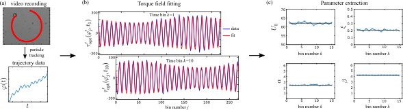
In the experiments, we placed a single particle on the ring and recorded a video for 30 min at a time resolution of 30 frames per second (). The video is analyzed by a particle tracking algorithm that outputs a two-dimensional trajectory. After conversion to polar coordinates, we obtain two time series and . Because of the strong radial confinement, we proceed by only analyzing . After transforming to the corotating frame,
| (16) |
we determined from Eq. (15).
The mobility in Eq. (15) was obtained independently from measurements of the time-dependent mean-square displacements in the absence of the optical force fields, which yielded the diffusion coefficient .
Figure 2(a) illustrates the particle tracking and Figure 2(b) shows representative results for the torque at two different times in the corotating frame, see the blue lines in the graph for and . The data show a deviation from the ideal travelling wave form, i.e. the sinus function for the torque in the corotating frame.
This deviation is likely caused by a non-flat amplitude response of the AOD in the deflection space. Such an imperfection can destroy the -periodicity of the optical potential but the potential must still be -periodic with respect to . Considering the potential barrier to be a general -periodic function of , we may take the first term of a Fourier expansion to describe the modified potential shape. This gives
| (17) |
in the laboratory frame, and
| (18) |
in the corotating frame. According to Eq. (17), the barrier height is modulated with a strength , and thus represents a mean barrier height.
For comparison with the torque data in Fig. 2, we must consider phase shifts and for both the periodic trap arrangement and the amplitude modulation. Taking the time instant , the shift accounts for the phase difference between the maxima of the function and an arbitrary but fixed zero point of along the ring in Fig. 1(b). Likewise, the shift accounts for the phase difference between the maximum of the barrier height modulation and the zero point. In the corotating frame we then have
| (19) |
and
| (20) | ||||
To determine the yet unknown parameters , , and , we fitted Eq. (20) to the experimental data for each time bin. The results are shown in Fig. 2(c). For all parameters we obtain constant values up to very small numerical uncertainties, which demonstrates that the functional form (19) is accurately representing the optical potential.
We critically checked the procedure of determining the optical potential by generating simulated data replacing the experimental ones. The corresponding simulations were performed for the Brownian dynamics of a single particle in the potential (19) with the parameters estimated from the measured trajectories in Fig. 2(c). Particle trajectories in these simulations were recorded with the same time resolution as in the experiment, and the procedure described above was applied to evaluate the potential parameters.
We found that all parameters agreed with the ones estimated from the experimental trajectories except of , which was underestimated by a few precent. The reason for this underestimation is that the time resolution in the experiment was not fully sufficient ( a bit too large). When using a higher time resolution in the generation of the data, the procedure for determining the potential parameters was giving the correct value for also. Figure 3 shows that the simulated (solid line) agree well with the measured ones (symbols).
IV Stokesian dynamics simulations
The driven Brownian motion of the colloidal particles can be described by the Langevin equations
| (21) |
where is a vector describing Gaussian white noise processes with zero mean and covariance matrix in accordance with the fluctuation-dissipation theorem, i.e. . The mobility tensor describes the force on particle mediated by the flow fields generated by the other particles as well as flow-effects mediated by the coverslip surface. It depends on the positions of the other particles and the distance from the surface.
For point particles and a flat surface with no-slip boundary conditions, is given by the Blake tensor Blake 1971. The entrainment of the fluid due to the finite size of the colloidal particles can be accounted for by a multipole expansion. Its truncation at the second order yields the Rotne-Prager level of the Blake tensor von Hansen et al. 2011. The respective formulas for are given in the Appendix.
In a reference frame corotating with the optical traps, the particles are dragged by the surrounding fluid and their Brownian dynamics become flow-driven. To see this, let us transform Eq. (21) into the corotating frame, where we denote the particle positions by . The transformation of the positions between laboratory and comoving frame is given by . Accordingly, we obtain
| (22) | ||||
where the prime in means to take the derivative with respect to the primed coordinates, , and are the elements of the mobility tensors as functions of the primed coordinates in the corotating frame. The first term on the right hand side of the equations corresponds to a vortex fluid field driving the particles in the azimuthal direction.
With the expression for the mobility tensor given in Appendix A, its divergence reduces to a simple derivative with respect to the distance of the particles from the coverslip surface. The equations of motions (21) thus become
| (23) |
In the experiments, we found that the particles are at a distance from the coverslip surface with only small fluctuations in the -direction. Here
| (24) |
is the distance between neighboring optical traps, that is the wavelength of the optical potential. In the simulations, we fixed for all , implying that the second term on the right hand side of Eq. (23) does not influence the dynamics.
As we can neglect the motion in radial direction also, see the discussion after Eq. (2), we project Eq. (23) onto the azimuthal direction, i.e. onto the axis given by the unit vector . We thus obtain the following equations of motions for the azimuthal angles,
| (25) |
The total force given by the sum in this equation is evaluated from the particle positions in the -plane at . Note that for weaker confining potentials in the radial direction, a HI induced particle pairing was reported, where the two particles forming pairs align almost along the radial direction Sokolov et al. 2011. However, in our experiments we did not observe any indication of such pairing, see also the videos referred to in Sec. III.1 after Eq. (2).
In the corotating frame, Eq. (25) becomes, with [ is the unit vector in -direction, see Fig. 1(b)],
| (26) |
The hard-sphere interaction implies that the distances between neighboring particles cannot be smaller than and that the particles keep their order (single-file transport). These constraints are taken into account in the simulation by the procedure proposed by Scala et al. Scala et al. 2007 and adopted to periodic potentials Ryabov et al. 2019.
V HI induced enhancement of barriers and implications for jamming
Simulations for the system with radius were carried out with and without consideration of HI. Figure 4 shows current-density relations obtained from these simulations for various barrier heights in a range investigated in the experiments. The density is given by the filling factor of the traps,
| (27) |
The currents were obtained from particle trajectories in the many-body system by first determining azimuthal velocities over time for all particles (same in experiments). After averaging, we obtain the mean velocity in azimuthal direction and the current . We normalized these currents with respect to
| (28) |
which is the single-particle current times the number of traps; is the mean single-particle velocity shown in Fig. 3. The multiplication with implies that for independent particles. Accordingly, the simulated currents in Fig. 4 approach the solid black line with slope one for small .
It is important to note that the currents in Fig. 4 are the ones in the corotating frame, i.e. the currents were determined based on Eq. (26). In particular, this means that in the absence of the optical potential, the particles would rotate counterclockwise with an angular velocity . For an optical potential with very high barriers, where the particles are carried along with the rotating traps, the current would be zero.
Comparing the results with and without HI shows that the presence of the HI is decisive for a suppression of the current at high particle densities to occur, as it is seen also in the experiments, see Fig. 4. In the absence of HI, the currents increase with density at large , which can be attributed to a cluster speed-up effects discussed in Refs. Antonov et al. 2022a; Antonov et al. 2022b; Lips et al. 2021.
How can we understand that HIs lead to a slowing down of the particle transport and a jamming behavior for large at high densities? To answer this question, we estimate how the HI modifies the motion for a particle that is typically close to the minimum of an optical trap and that has two neighbors at a distance of about , i.e. close to the trap minima next to it. As the mobilities in Eq. (25) decrease with distance, we consider the sum of HI induced forces to be dominated by the contribution of these neighboring particles. Also, we neglect the relatively weak flow effects caused by the coverslip surface, i.e. we use the mobility tensors at the Rotne-Prager level with components
| (29) |
Here , and the non-diagonal term follows from Eq. (A8) when taking into account according to Stokes friction law ( is the dynamic viscosity).
The particle and the two neighboring ones at distance are located essentially along a line (for neighboring traps, the curvature of the ring can be neglected) and the optical forces exerted on them are almost in the direction of this line. We thus approximate the sum in Eq. (25) by considering a one-dimensional geometry in a direction , yielding
| (30a) | ||||
| (30b) | ||||
When going from the second to the third line we used that the particles have mutual distances and that the optical potential is -periodic. As depends only on the distance between particles, we used also . Inserting the diagonal element of from Eq. (29), we obtain
| (31) |
In the absence of HI, only the first term equal to the one in the bracket on the right hand side of Eq. (31) would be present. For our estimate based on the Rotne-Prager expression for the mobility tensor, the particle radius should be significantly smaller than . In this regime, the additional two terms in the bracket give an additional contribution larger than zero. For the radius , we have , and the bracket gives a value of about two. This means that the optical potential has an effectively higher mean barrier height . It is intuitively clear that such barrier enhancement should slow down the motion but it is not immediately evident why it leads to the jamming behavior.
The jamming like behavior can be understood from the effective mean external potential in the azimuthal direction in the corotating frame. In the absence of the driving, this potential is given by from Eq. (7) with an HI-enhanced barrier height (and we set the irrelevant constant ). The flow-driving given by in Eq. (22) corresponds to a constant torque . Accordingly, becomes tilted in -direction, i.e.
| (32) |
For a given tilt, as in our experiment, this potential exhibits minima only for sufficiently large barrier heights, i.e. in the regime commonly referred to as undercritical tilting. In that case, potential wells exist that, when occupied by a particle, form an obstacle for the motion of nearby particles (blocking effect) and lead to jamming at high particle densities.
Figure 5 shows the transition from over- to undercritical tilting for the potential in Eq. (32). For smaller than a critical , the particles can slide down in the -direction, while for they have to surmount potential barriers in thermally activated rare events. The critical barrier for passing from over- to undercritical tilting with increasing is . Accordingly, due to the HI-enhanced barrier height, the regime of undercritical tilting can occur already for much smaller than the critical value, and this leads to jamming at large for comparatively small barrier heights, see Fig. 4.
According to the estimate in Eq. (31), the barrier enhancement should increase with the ratio for , see the inset of Fig. 5, where we show . As a consequence, we expect the transition from over- to undercritical tilting to shift towards smaller barrier heights with decreasing or decreasing ring radius [see Eq. (24)].
To test this, we have carried out other experiments and corresponding simulations for two other radii and . To keep the tilting in Eq. (32) and hence the drag torque on the particles constant, we adjusted for each radius such that remains constant. The results for the current-density relations (fundamental diagrams) for all three studied radii are shown in Fig. 6. In the upper row, the experimental results are displayed. For all three radii, a jamming behavior is seen at large and sufficiently strong barrier height . When comparing curves for similar barrier heights, one notices that the jamming becomes more pronounced for smaller radii or larger ratios . The corresponding simulated results in Fig. 6 show an analogous behavior.
In particular, the onset of the jamming behavior is shifted in agreement with our expectation: For () it occurs at a barrier height of about , while for () it is at a higher . The shift given by the term in parentheses on the right-hand side of Eq. (31) would be smaller than this, but we should not expect to obtain a quantitative agreement from our simple estimate.
When comparing experimental and simulated data for the same values, we see also that there is no quantitative match. This can be due to the simplifications in our modeling, where we have considered the particle motion to be perfectly confined along the azimuthal direction, and where we treated the HIs approximately by the Blake tensor at the Rotne-Prager level.
VI Flow-driven versus force-driven systems
As mentioned in the introduction, previous findings reported on a barrier reduction effect induced by HIs. These findings were obtained for force-driven systems. For our setup, we have performed simulations also when the particles are driven by a force instead of a flow. In these simulations, we have also switched off the amplitude modulation, which is not a crucial factor for our results reported above. The fundamental diagrams obtained from these simulations are shown in Fig. 7. In the flow-driven system, the jamming behavior is seen in the presence of HI. In the absence of HI, we obtain even a current enhancement compared to at larger particle densities. This can be explained by the fact that the effective potential in Eq. (32) has steep slopes (large driving forces) in certain regions. When increasing the density , these regions with large driving forces become more strongly populated, leading to the enhancement of the current.
In the force-driven system by contrast, the results in Fig. 7 do not reflect a jamming behavior in the presence of HI and the currents are much larger. Why are the currents so much different compared to a flow-driven system?
In the force-driven case, we have a drag force acting on particle . The equations of motion (22) then become
| (33) |
For the comparison with the flow-driven system, we can ignore the experimental way of generating the flow-driving, i.e. disregard the prime on the coordinates in Eq. (22). The effect of the mobility tensors on these drag forces would then be the same as on the forces of the optical potential, implying that both the barrier height and the drag force amplitude are enhanced by a factor as estimated in Eq. (31). This means that no transition between the regimes of over- and undercritical is occuring with increasing . Instead, the system stays in the regime of overcritical tilting and the density dependence of the current is almost unaffected when changing .
The much higher currents in the force-driven system compared to the flow-driven one can be understood from the fact that the mean barrier height and drag force amplitude are enhanced by HI in the same manner. When neglecting the divergences of the mobility tensors and when taking into account that the experimental conditions refer to a situation of low noise (), the enhancement amounts to a mere speeding-up of all velocities by the same factor. This is not the case in the flow- driven system, where the amplitudes of the optical forces are HI-enhanced but not that of the flow-driving forces .
VII Summary and conclusions
Transport over potential barriers is omnipresent in nature. Here we have reported experimental and theoretical results on the question how HIs influence such transport in the case of Brownian motion of hard spheres in a periodic potential.
In our experiments we designed a setup of rotating optical traps that allowed us to study the particle transport under a vortex flow-field. For deep optical traps, we found that the currents strongly decrease with the particle density, reflecting a jamming behavior. Stokesian dynamics simulations of the setup showed that this behavior is caused by HIs. We interpreted this finding by an effective HI-induced enhancement of the barriers between the optical traps, which leads to a transition from an overcritical to an undercritical tilting of the optical potential. The enhancement is contrary to what has been reported for the impact of HI on potential barriers in force-driven systems. Comparison of flow- to force-driving in our setup also shows striking differences. They are caused by an effective enhancement of the force amplitude going along with the barrier increase. As a consequence, no transition of the tilting characteristics is induced by the HI and the currents are only weakly affected by the depths of the optical traps.
Our interpretation for the jamming as a consequence of a HI-induced transition from over- to undercritical tilting of the optical potential provides an understanding of the observed behavior. The formula (31) derived for estimating the HI- induced barrier enhancement, however, should not be considered as giving quantitative predictions. To this end, the theoretical treatment needs to be improved.
One possible improvement concerns the consideration of fluctuations in particle positions and of particles at distances beyond neighboring potential wells. Another concerns the Rotne-Prager level of description, even when taking into account the additional terms in the Blake tensor to account for the flow effects from the coverslip surface. Not considered yet are in particular effects when particles come close to each other, which would require to take into account terms of higher order in the multipole expansion of mobilities and lubrication effects associated with a rotational motion of the particles. This can be done based on the mobility method by using the expressions derived in Ref. Durlofsky et al. 1987 for lubrication forces between the particles, and in Ref. Swan and Brady 2007 to take into account lubrication effects of the particles with the coverslip. Another possible approach is to resort to large-scale simulation methods with explicit modeling of fluid flows in multiparticle collision dynamics Howard et al. 2019.
From the experimental side, the explored system can be extended in various ways. For example, the present work is centered on the flow-driven properties of monodisperse systems. One could ask how the collective dynamics and the reported jamming effect are altered in polydisperse systems with particles of different sizes. The simplest case would be to include one or few differently sized particles within the ring and investigate how these inclusions behave by varying their relative fraction and the depth of the potential wells. Smaller or larger particles will see a different potential well than their neighbors, and this will affect their jumping over the potential barriers.
Further, modern colloid science allows to prepare monodisperse particles with a shape that departs from the spherical one, such as ellipsoids Champion et al. 2007 or even cubes Rossi et al. 2010. Using anisotropic colloids will increase the complexity of the system when considering the generated HIs but, on the other hand, will allow one to extract experimentally also the relative orientation of the particles within the ring. This further piece of information could be used to determine whether, in the steady state, such particles synchronize their rotational motion due to HIs under the driving.
The nature of the particles can also be changed, for example by using monodisperse paramagnetic colloids, which could be easily manipulated via magnetic fields in this geometry Ortiz-Ambriz et al. 2018; Gerloff et al. 2020. One could increase the density of particles to induce jamming, but use a rotating field Tierno et al. 2007; Martinez-Pedrero et al. 2015 with opposite chirality to apply a torque which would un-jam the system.
Finally, instead of changing the particles, the AOD can be programmed in such a way to introduce a controlled degree of spatial or temporal disorder in the potential landscape, for example by reducing or increasing the time that the laser beam visits one trap. One can also design more complex optical paths than the circular one, like elliptical or square where the presence of sharp corners could induce earlier the jamming behavior or could act as a sink of particles to be later released at high angular speed.
Exploring these interesting options will foster our understanding of HI effects in natural systems and could open ways towards their exploitation in technological applications.
Acknowledgements
We sincerely thank G. Nägele and H. Stark for advice on the treatment of hydrodynamic interactions. This project has received funding from the European Research Council (ERC) under the European Union’s Horizon 2020 research and innovation program (grant agreement no. 811234). P.T. acknowledges support from the Generalitat de Catalunya under Program “ICREA Acadèmia”. A.R. and P.M. gratefully acknowledge financial support by the Czech Science Foundation (Project No. 20-24748J) and the Deutsche Forschungsgemeinschaft (Project Nos. 397157593, 355031190). We sincerely thank the members of the DFG Research Unit FOR 2692 for fruitful discussions.
APPENDIX
Appendix A Blake tensor at the
Rotne-Prager level von Hansen et al. 2011
The Blake tensor at the Rotne-Prager level decomposes into a self and an interaction part,
| (A1) |
The self part depends only on the distance of a particle from the coverslip surface,
| (A2) |
| (A3a) | |||
| (A3b) |
The interaction part is given by the “curvature correction” (second order term of multipole expansion) of the Blake tensor,
| (A4) |
The Blake tensor is
| (A5) |
where , and is the Oseen tensor, the Stokes doublet, and the source doublet. These tensors are given by
| (A6a) | ||||
| (A6b) | ||||
| (A6c) | ||||
where , , and is the dynamic viscosity ( in the experiment with the kinematic viscosity of water).
The explicit expression for is
| (A7) |
where
| (A8) |
| and has diagonal components () | |||
| (A9a) | |||
| (A9b) | |||
| and off-diagonal elements (, ) | |||
| (A9c) | |||
| (A9d) | |||
| (A9e) | |||
References
- Happel and Brenner (1973) J. Happel and H. Brenner, Low Reynolds Number Hydrodynamics (Noordhoff, Leiden, Noordhoff, 1973).
- Dhont (1996) J. K. G. Dhont, An Introduction to Dynamics of Colloids (Elsevier, Amster- dam, Boston, 1996).
- Hess and Klein (2006) W. Hess and R. Klein, Generalized hydrodynamics of systems of Brownian particles, Rep. Prog. Phys. 71, 173 (2006).
- Lauga and Powers (2009) E. Lauga and T. R. Powers, The hydrodynamics of swimming microorganisms, Rep. Prog. Phys. 72, 096601 (2009).
- Riedel et al. (2005) I. H. Riedel, K. Kruse, and J. Howard, A self-organized vortex array of hydrodynamically entrained sperm cells., Science 309, 300 (2005).
- Pierce et al. (2018) C. J. Pierce, H. Wijesinghe, E. Mumper, B. H. Lower, S. K. Lower, and R. Sooryakumar, Hydrodynamic interactions, hidden order, and emergent collective behavior in an active bacterial suspension, Phys. Rev. Lett. 121, 188001 (2018).
- Lauga et al. (2006) E. Lauga, W. R. DiLuzio, G. M. Whitesides, and H. A. Stone, Swimming in circles: Motion of bacteria near solid boundaries., Biophys. J. 90, 400 (2006).
- Berke et al. (2008) A. P. Berke, L. Turner, H. C. Berg, and E. Lauga, Hydrodynamic attraction of swimming microorganisms by surfaces, Phys. Rev. Lett. 101, 038102 (2008).
- Di Leonardo et al. (2011) R. Di Leonardo, D. Dell’Arciprete, L. Angelani, and V. Iebba, Swimming with an image, Phys. Rev. Lett. 106, 038101 (2011).
- Reichert and Stark (2005) M. Reichert and H. Stark, Synchronization of rotating helices by hydrodynamic interactions, Eur. Phys. J. E 17, 493 (2005).
- Vilfan and Jülicher (2006) A. Vilfan and F. Jülicher, Hydrodynamic flow patterns and synchronization of beating cilia, Phys. Rev. Lett. 96, 058102 (2006).
- Drescher et al. (2009) K. Drescher, K. C. Leptos, I. Tuval, T. Ishikawa, T. J. Pedley, and R. E. Goldstein, Dancing volvox: Hydrodynamic bound states of swimming algae, Phys. Rev. Lett. 102, 168101 (2009).
- Uchida and Golestanian (2011) N. Uchida and R. Golestanian, Generic conditions for hydrodynamic synchronization, Phys. Rev. Lett. 106, 058104 (2011).
- Brumley et al. (2012) D. R. Brumley, M. Polin, T. J. Pedley, and R. E. Goldstein, Hydrodynamic synchronization and metachronal waves on the surface of the colonial alga volvox carteri, Phys. Rev. Lett. 109, 268102 (2012).
- Chakrabarti and Saintillan (2019) B. Chakrabarti and D. Saintillan, Hydrodynamic synchronization of spontaneously beating filaments, Phys. Rev. Lett. 123, 208101 (2019).
- Crocker and Grier (1996) C. Crocker and D. G. Grier, Methods of digital video microscopy for colloidal studies, J. Coll. Int. Sci. 179, 298 (1996).
- Baumgartl and Bechinger (2005) J. Baumgartl and C. Bechinger, On the limits of digital video microscopy, Europhys. Lett. 71, 487 (2005).
- Qiu et al. (1990) X. Qiu, X. L. Wu, J. Z. Xue, D. J. Pine, D. A. Weitz, and P. M. Chaikin, Hydrodynamic interactions in concentrated suspensions, Phys. Rev. Lett. 65, 516 (1990).
- Zahn et al. (1997) K. Zahn, J. M. Méndez-Alcaraz, and G. Maret, Hydrodynamic Interactions May Enhance the Self-Diffusion of Colloidal Particles, Phys. Rev. Lett. 79, 175 (1997).
- Nägele and Baur (1997) G. Nägele and P. Baur, Influence of hydrodynamic interactions on long-time diffusion in charge-stabilized colloids, Europhys. Lett. 38, 557 (1997).
- Rinn et al. (1999) B. Rinn, K. Zahn, P. Maass, and G. Maret, Influence of hydrodynamic interactions on the dynamics of long-range interacting colloidal particles, Europhys. Lett. (EPL) 46, 537 (1999).
- Härtl et al. (2000) W. Härtl, J. Wagner, C. Beck, F. Gierschner, and R. Hempelmann, Self-diffusion and hydrodynamic interactions in highly charged colloids, J. Phys.: Condens. Matter 12, 287 (2000).
- Riese et al. (2000) D. O. Riese, G. H. Wegdam, W. L. Vos, R. Sprik, D. Fenistein, J. H. H. Bongaerts, and G. Grübel, Effective screening of hydrodynamic interactions in charged colloidal suspensions, Phys. Rev. Lett. 85, 5460 (2000).
- Santana-Solano and Arauz-Lara (2001) J. Santana-Solano and J. L. Arauz-Lara, Hydrodynamic interactions in quasi-two-dimensional colloidal suspensions, Phys. Rev. Lett. 87, 038302 (2001).
- Banchio et al. (2006) A. J. Banchio, J. Gapinski, A. Patkowski, W. Häußler, A. Fluerasu, S. Sacanna, P. Holmqvist, G. Meier, M. P. Lettinga, and G. Nägele, Many-body hydrodynamic interactions in charge-stabilized suspensions, Phys. Rev. Lett. 96, 138303 (2006).
- Segrè et al. (1997) P. N. Segrè, E. Herbolzheimer, and P. M. Chaikin, Long-range correlations in sedimentation, Phys. Rev. Lett. 79, 2574 (1997).
- Segré et al. (2001) P. N. Segré, F. Liu, P. Umbanhowar, and D. A. Weitz, An effective gravitational temperature for sedimentation, Nature 409, 594 (2001).
- Padding and Louis (2004) J. T. Padding and A. A. Louis, Hydrodynamic and Brownian fluctuations in sedimenting suspensions, Phys. Rev. Lett. 93, 220601 (2004).
- Cui et al. (2002) B. Cui, H. Diamant, and B. Lin, Screened hydrodynamic interaction in a narrow channel, Phys. Rev. Lett. 89, 188302 (2002).
- Cui et al. (2004) B. Cui, H. Diamant, B. Lin, and S. A. Rice, Anomalous hydrodynamic interaction in a quasi-two-dimensional suspension, Phys. Rev. Lett. 92, 258301 (2004).
- Xu et al. (2005) X. Xu, S. A. Rice, B. Lin, and H. Diamant, Influence of hydrodynamic coupling on pair diffusion in a quasi-one-dimensional colloid system, Phys. Rev. Lett. 95, 158301 (2005).
- Grzybowski et al. (2000) B. A. Grzybowski, H. A. Stone, and G. M. Whitesides, Dynamic self-assembly of magnetized, millimetre-sized objects rotating at a liquid-air interface, Nature 405, 1033 (2000).
- Lenz et al. (2003) P. Lenz, J.-F. m. c. Joanny, F. Jülicher, and J. Prost, Membranes with rotating motors, Phys. Rev. Lett. 91, 108104 (2003).
- Radu and Schilling (2014) M. Radu and T. Schilling, Solvent hydrodynamics speed up crystal nucleation in suspensions of hard spheres, Europhys. Lett. 105, 26001 (2014).
- Tateno et al. (2019) M. Tateno, T. Yanagishima, J. Russo, and H. Tanaka, Influence of hydrodynamic interactions on colloidal crystallization, Phys. Rev. Lett. 123, 258002 (2019).
- Reichert and Stark (2004) M. Reichert and H. Stark, Circling particles and drafting in optical vortices, J. Phys.: Condens. Matter 16, S4085 (2004).
- Lutz et al. (2006) C. Lutz, M. Reichert, H. Stark, and C. Bechinger, Surmounting barriers: The benefit of hydrodynamic interactions, EPL 74, 719 (2006).
- Beatus et al. (2007) T. Beatus, R. Bar-Ziv, and T. Tlusty, Anomalous microfluidic phonons induced by the interplay of hydrodynamic screening and incompressibility, Phys. Rev. Lett. 99, 124502 (2007).
- Beatus et al. (2009) T. Beatus, T. Tlusty, and R. Bar-Ziv, Burgers shock waves and sound in a 2D microfluidic droplets ensemble, Phys. Rev. Lett. 103, 114502 (2009).
- Grimm and Stark (2011) A. Grimm and H. Stark, Hydrodynamic interactions enhance the performance of Brownian ratchets, Soft Matter 7, 3219 (2011).
- Malgaretti et al. (2012) P. Malgaretti, I. Pagonabarraga, and D. Frenkel, Running faster together: Huge speed up of thermal ratchets due to hydrodynamic coupling, Phys. Rev. Lett. 109, 168101 (2012).
- Dobnikar et al. (2013) J. Dobnikar, A. Snezhko, and A. Yethiraj, Emergent colloidal dynamics in electromagnetic fields, Soft Matter 9, 3693 (2013).
- Nagar and Roichman (2014a) H. Nagar and Y. Roichman, Collective excitations of hydrodynamically coupled driven colloidal particles, Phys. Rev. E 90, 042302 (2014a).
- Martínez-Pedrero and Tierno (2018) F. Martínez-Pedrero and P. Tierno, Advances in colloidal manipulation and transport via hydrodynamic interactions, J. Colloid Interface Sci. 519, 296 (2018).
- Misiunas and Keyser (2019) K. Misiunas and U. F. Keyser, Density-dependent speed-up of particle transport in channels, Phys. Rev. Lett. 122, 214501 (2019).
- Meiners and Quake (1999) J.-C. Meiners and S. R. Quake, Direct measurement of hydrodynamic cross correlations between two particles in an external potential, Phys. Rev. Lett. 82, 2211 (1999).
- Dufresne et al. (2000) E. R. Dufresne, T. M. Squires, M. P. Brenner, and D. G. Grier, Hydrodynamic coupling of two Brownian spheres to a planar surface, Phys. Rev. Lett. 85, 3317 (2000).
- Martin et al. (2006) S. Martin, M. Reichert, H. Stark, and T. Gisler, Direct observation of hydrodynamic rotation-translation coupling between two colloidal spheres, Phys. Rev. Lett. 97, 248301 (2006).
- Kotar et al. (2013) J. Kotar, L. Debono, N. Bruot, S. Box, D. Phillips, S. Simpson, S. Hanna, and P. Cicuta, Optimal hydrodynamic synchronization of colloidal rotors, Phys. Rev. Lett. 111, 228103 (2013).
- Kreiserman et al. (2019) R. Kreiserman, O. Malik, and A. Kaplan, Decoupling conservative forces and hydrodynamic interactions between optically trapped spheres, Phys. Rev. E 99, 012611 (2019).
- Ladavac and Grier (2005) K. Ladavac and D. G. Grier, Colloidal hydrodynamic coupling in concentric optical vortices, Europhys. Lett. 70, 548 (2005).
- Polin et al. (2006) M. Polin, D. G. Grier, and S. R. Quake, Anomalous vibrational dispersion in holographically trapped colloidal arrays, Phys. Rev. Lett. 96, 088101 (2006).
- Cereceda-López et al. (2021) E. Cereceda-López, D. Lips, A. Ortiz-Ambriz, A. Ryabov, P. Maass, and P. Tierno, Hydrodynamic interactions can induce jamming in flow-driven systems, Phys. Rev. Lett. 127, 214501 (2021).
- Kim and Karrila (1991) S. Kim and S. J. Karrila, Microhydrodynamics: Principles and Selected Appliacations (Butterworth-Heinemann, Boston, 1991).
- Nagar and Roichman (2014b) H. Nagar and Y. Roichman, Collective excitations of hydrodynamically coupled driven colloidal particles, Phys. Rev. E 90, 042302 (2014b).
- Sassa et al. (2012) Y. Sassa, S. Shibata, Y. Iwashita, and Y. Kimura, Hydrodynamically induced rhythmic motion of optically driven colloidal particles on a ring, Phys. Rev. E 85, 061402 (2012).
- (57) Videos demonstrating the negligible particle motion in radial direction can be found at doi:10.1103/PhysRevLett.127.214501.
- Juniper et al. (2016) M. P. N. Juniper, A. V. Straube, D. G. A. L. Aarts, and R. P. A. Dullens, Colloidal particles driven across periodic optical-potential-energy landscapes, Phys. Rev. E 93, 012608 (2016).
- Juniper et al. (2012) M. P. N. Juniper, R. Besseling, D. G. A. L. Aarts, and R. P. A. Dullens, Acousto-optically generated potential energy landscapes: Potential mapping using colloids under flow, Opt. Express 20, 28707 (2012).
- Risken (1985) H. Risken, The Fokker-Planck Equation: Methods of Solution and Applications (Springer-Verlag Berlin, 1985).
- Blake (1971) J. R. Blake, A note on the image system for a stokeslet in a no-slip boundary, Math. Proc. Camb. Philos. Soc. 70, 303 (1971).
- von Hansen et al. (2011) Y. von Hansen, M. Hinczewski, and R. R. Netz, Hydrodynamic screening near planar boundaries: Effects on semiflexible polymer dynamics, J. Chem. Phys. 134, 235102 (2011).
- Sokolov et al. (2011) Y. Sokolov, D. Frydel, D. G. Grier, H. Diamant, and Y. Roichman, Hydrodynamic pair attractions between driven colloidal particles, Phys. Rev. Lett. 107, 158302 (2011).
- Scala et al. (2007) A. Scala, T. Voigtmann, and C. De Michele, Event-driven Brownian dynamics for hard spheres, J. Chem. Phys. 126, 134109 (2007).
- Ryabov et al. (2019) A. Ryabov, D. Lips, and P. Maass, Counterintuitive short uphill transitions in single-file diffusion, J. Phys. Chem. C 123, 5714 (2019).
- Antonov et al. (2022a) A. P. Antonov, A. Ryabov, and P. Maass, Solitons in overdamped Brownian dynamics, Phys. Rev. Lett. 129, 080601 (2022a).
- Antonov et al. (2022b) A. P. Antonov, D. Voráč, A. Ryabov, and P. Maass, Collective excitations in jammed states: ultrafast defect propagation and finite-size scaling, New J. Phys. 24, 093020 (2022b).
- Lips et al. (2021) D. Lips, R. L. Stoop, P. Maass, and P. Tierno, Emergent colloidal currents across ordered and disordered landscapes, Commun. Phys. 4, 224 (2021).
- Durlofsky et al. (1987) L. Durlofsky, J. F. Brady, and G. Bossis, Dynamic simulation of hydrodynamically interacting particles, J. Fluid Dyn. 180, 21 (1987).
- Swan and Brady (2007) J. W. Swan and J. F. Brady, Simulation of hydrodynamically interacting particles near a no-slip boundary, Phys. Fluids 19, 113306 (2007).
- Howard et al. (2019) M. P. Howard, A. Nikoubashman, and J. C. Palmer, Modeling hydrodynamic interactions in soft materials with multiparticle collision dynamics, Curr. Opin. Chem. Eng. 23, 34 (2019).
- Champion et al. (2007) J. A. Champion, Y. K. Katare, and S. Mitragotri, Making polymeric micro- and nanoparticles of complex shapes, Proc. Natl. Acad. Sci. U. S.A. 104, 11901 (2007).
- Rossi et al. (2010) L. Rossi, S. Sacanna, W. T. M. Irvine, P. M. Chaikin, D. J. Pine, and A. P. Philipse, Cubic crystals from cubic colloids, Soft Matter 7, 4139 (2010).
- Ortiz-Ambriz et al. (2018) A. Ortiz-Ambriz, S. Gerloff, S. H. L. Klapp, J. Ortín, and P. Tierno, Laning, thinning and thickening of sheared colloids in a two-dimensional Taylor–Couette geometry, Soft Matter 14, 5121 (2018).
- Gerloff et al. (2020) S. Gerloff, A. Ortiz-Ambriz, P. Tierno, and S. H. L. Klapp, Dynamical modes of sheared confined microscale matter, Soft Matter 16, 9423 (2020).
- Tierno et al. (2007) P. Tierno, R. Muruganathan, and T. M. Fischer, Viscoelasticity of dynamically self-assembled paramagnetic colloidal clusters, Phys. Rev. Lett. 98, 028301 (2007).
- Martinez-Pedrero et al. (2015) F. Martinez-Pedrero, A. Ortiz-Ambriz, I. Pagonabarraga, and P. Tierno, Colloidal microworms propelling via a cooperative hydrodynamic conveyor belt, Phys. Rev. Lett. 115, 138301 (2015).