A Two-phase On-line Joint Scheduling for Welfare Maximization of Charging Station
Abstract
The large adoption of EVs brings practical interest to the operation optimization of the charging station. The joint scheduling of pricing and charging control will achieve a win-win situation both for the charging station and EV drivers, thus enhancing the operational capability of the station. We consider this important problem in this paper and make the following contributions. First, a joint scheduling model of pricing and charging control is developed to maximize the expected social welfare of the charging station considering the Quality of Service and the price fluctuation sensitivity of EV drivers. It is formulated as a Markov decision process with variance criterion to capture uncertainties during operation. Second, a two-phase on-line policy learning algorithm is proposed to solve this joint scheduling problem. In the first phase, it implements event-based policy iteration to find the optimal pricing scheme, while in the second phase, it implements scenario-based model predictive control for smart charging under the updated pricing scheme. Third, by leveraging the performance difference theory, the optimality of the proposed algorithm is theoretically analyzed. Numerical experiments for a charging station with distributed generation and energy storage demonstrate the effectiveness of the proposed method and the improved social welfare of the charging station.
Index Terms:
Electric vehicle, Markov decision process, discrete event dynamic systems, event-based optimization.I Introduction
Acting as the main hinge between transportation sector and power sector, electric vehicles (EVs) attract more and more attention in recent years. On one hand, the EVs will largely reduce the carbon emission of the transportation sector if they are supplied by clean energy, such as wind power, solar power, etc. On the other hand, the EVs can be used as mobile storage to increase the demand elasticity in the power sector. Due to these reasons, many countries have made incentive policy to stimulate the EV market. For example, as the world’s largest EV market, several cities in China, such as Beijing, Shenzhen, are subsidizing to accelerate the shift to electric taxi and it is estimated that there will be over 300 thousand electric taxies until 2020[1].
The main influential factors for the popularization of EVs lie in two aspects. The first is the charging price which is the main focus of the EV drivers, especially for electric taxi drivers. The current unsustainable low price for EV charging comes from various incentive subsidies comparing with relatively expensive oil price [2]. Another is the charging control which is the main focus of the charging station. Existing literatures have shown that disorderly charging will incur increased operation cost of the charging station and may bring in damages to the power grid [3]. Luckily, these factors can also be controlled by the charging station. Therefore, it is of great practical interest for the charging station to optimize the charging price and implement smart charging control for the EVs in order to achieve a win-win situation for both the charging station and EV drivers.
However, this problem usually faces the following challenges. First, the uncertainties in the charging behavior of EV drivers. The charging price scheme will influence the EV driver’s decision to enter for charging and each driver has different response to the charging price scheme. Furthermore, the arrival time, required charging energy and parking time of EVs are all uncertain before parking to charge. Second, the tradeoff between maximizing operation profit and minimizing the charging cost. The low charging price will attract more EVs to enter for charging, however the operation profit may be reduced for the charging station. On the contrary, the high charging price may gain the high unit profit per EV, but the total operation profit may be low as the service number will be reduced due to high charging price. Third, the price fluctuation sensitivity of EV drivers. The EV drivers are serious and sensitive to the price fluctuation. Although the large price fluctuation of the charging station may increase the operation profit, it will also bring in uncertainties and variation of charging cost for the EV drivers. This may incur reduced preference to choose this charging station for EV drivers. Fourth, the multi-stage coupled relationship between pricing and charging control. The current charging price will influence the number of EVs to be charged and further influence the charging control in the future considering the relative long charging time. The pricing and charging control should be jointly considered in a multi-stage decision fashion.
Based on the discussions above, we study the joint scheduling of pricing and charging control for the charging station in this paper. Compared with the published literature, the main contributions of this paper are as follows:
-
A joint scheduling model of pricing and charging control is developed to maximize the expected social welfare of the charging station considering the Quality of Service (QoS), the price fluctuation sensitivity of drivers and uncertain charging behaviors. This model is formulated as a Markov decision process (MDP) with variance criterion to capture uncertainties during operation.
-
A two-phase online policy learning method is proposed to solve this joint scheduling problem. In the first phase, an event-based policy iteration which alleviates the burden of large state/action space is developed to find the optimal pricing scheme. In the second phase, the scenario-based model predictive control (MPC) is developed to achieve smart charging under the updated pricing scheme.
-
The optimality of the proposed method is theoretically analyzed by leveraging performance difference theory. Numerical results for a typical charging station with distributed generation and energy storage demonstrate the effectiveness of the proposed optimization method and the improved social welfare of the charging station.
The rest of this paper is organized as follows. We briefly review the related literature in Section II, formulate the problem in Section III, present the solution methodology in Section IV, discuss the numerical results in Section V, and briefly conclude in Section VI.
II Literature Review
The charging control of EVs has attracted a lot of attention in recent years. In most of works, the charging price is assumed to be known and uncontrollable[4, 5, 6]. In this case, various charging control methods are proposed for charging process optimization, such as mixed-integer programming[7], model predictive control[8], reinforcement learning[9], etc. However, besides the charging process optimization, the pricing is another important control mechanism for the charging station to maximum its operation profit. The EV drivers and charging station will further benefit from the joint scheduling of pricing and charging control.
One of the traditional pricing mechanisms is to use price elastic matrix (PEM) to evaluate the charging demand response[10, 11]. The PEM is defined as the ratio of the change in charging demand to the base charging demand over the change in price to the base price. The optimal pricing scheme can be obtained by evaluating the pricing effect under the PEM criterion. However, the individual response to the price is neglected for each EV driver in this method. The individual response will influence the number of EVs which enter into the charging station and further influence the charging control of EVs.
Another important pricing mechanism is to use queue theory to implement dynamic/static pricing control[12, 13]. In [14], a M/M/C queue model is proposed to determine the discounted charging price to provide charging service deferral for charging demand shifting. In [15], an optimal pricing scheme is designed by formulating the dual-mode charging station as a queue network with multiple servers and heterogeneous service rate. In most of works, the arrival rate of EVs is assumed to be constant. As the drivers are price-sensitive, they may choose other charging stations when observing unsatisfactory charging price. In this way, the arrival rate of EVs will be time-varying.
The game theory is also a natural candidate for the pricing of EVs. In [16], the bi-level pricing scheme is obtained by formulating the competition among EV owners, the aggregator and the distribution system operator as the Stackelberg game. In [17], it considers the price competition problem among multiple charging stations as a game with incomplete information of the market environment. In [18], it introduces a game-theoretic algorithm to find a charging rate-dependent pricing mechanism which meets the charging demand at the minimum price. However, few consider the uncertainties in the charging behaviors of EVs. Furthermore, the game-based pricing method requires iterative computations to achieve Nash equilibrium which is time-consuming.
In conclusion, few existing literatures consider the individual response of EV drivers to the price and its impact to the charging control of EVs. Furthermore, to the best of the authors’ knowledge, the existing literatures have not considered the price fluctuation sensitivity of the EV drivers which affects the drivers’ satisfactory to the charging station. Also, most works do not consider the multi-stage coupled relationship between pricing and charging control with uncertain charging behaviors of EVs. Therefore, we will consider these in this paper.
III Problem Formulation
III-A System Description
We consider a charging station equipped with several charging piles, distributed renewable energy and energy storage as depicted in Fig. 1. The energy operator in the charging station is responsible to determine the pricing scheme and control the charging process of parked EVs. At each decision stage, the energy operator will announce the charging price to EVs based on the distributed energy generation prediction, the status of storage and parked EVs. Then, EVs will determine whether enter into this charging station to charge or not. If accept this charging price, the EVs will enter into the charging station and report their charging requests to the energy operator. Meanwhile, the energy operator should implement smart control for the parked EVs, distributed renewable energy and storage considering the distributed energy generation prediction, the status of storage and parked EVs. The energy operator can also procure electricity from the power grid in case of insufficient supply.
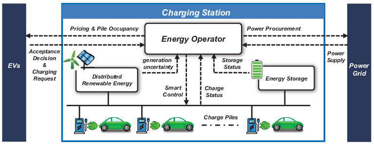
Considering this operation mechanism, the energy operator should jointly implement pricing and charging control of EVs to maximize its social welfare, including the operation profit, QoS and the price fluctuation. As there exists uncertainties in the charging behaviors of EV drivers and the generation of the distributed renewable energy, this problem is a multi-stage stochastic programming problem. In the following, we will use MDP to formulate this problem as it is an effective tool for sequential multi-objective decision-making problem under uncertainty[19]. To simplify the discussions, the fixed charging power is considered to prolong the battery life of EV.
III-B System Model
We consider this joint scheduling problem over the discretized horizon where denotes the decision epoch and denotes the decision interval. There are charging piles in the charging station. The MDP model of this joint scheduling problem is shown below.
1) System States: The system state at time is defined as where and denote the generation of the distributed wind energy and solar power, denotes the State of Charge (SOC) of storage, and denote the remaining required charging energy and remaining parking time of the EV in the th charging pile where and denotes the state space. When the th charging pile is unoccupied, there are and .
2) Actions: The control action at stage is defined as where denotes the charging price, denotes the power output of storage, is the control decision for the th charging pile and denotes the action space. denotes that the th charging pile will charge its connected EV, otherwise .
Motivated by [14], in order to encourage the EV drivers to join in the smart charging, the charging station will offer a charging price discount for the arrival EVs based on their charging elasticity, i.e., for the th charging pile which has newly arrival EV at stage , there is
| (1) |
where denotes the charging price for the EV which connected to the th charging pile from to , denotes the discount coefficient, denotes the charging elasticity of the connected EV, denotes its charging power and denotes the charging efficiency. It can be seen that the longer parking time and less required charging energy means the larger elasticity. Therefore, the charging price is cheaper. Note that each EV will decide whether enter into the charging station based on its time-invariant discounted price . When is determined, the charging cost will be known by the EV owners by multiplying with the known required charging energy.
3) System Dynamics: For the charging station, there is the following relationship for the number of parked EVs, i.e.,
| (2) |
where denotes the number of parked EVs at stage , denotes the number of newly arrival EVs which decide to enter into the charging station and denotes the number of departure EVs due to the end of parking at stage .
Based on the observation, the charging station can obtain the probability distribution of the number of newly arrival EVs. Usually, it can be assumed to follow poisson distribution with mean arrival rate at stage [20]. Once arrival, the EV driver will decide whether enter into the charging station based on the announced charging price and the availability of unoccupied charging piles. As EV drivers express difference preferences over the charging price, let denotes the acceptance probability of the charging price. Then, the probability distribution of satisfies
| (3) |
Based on [21], the Bernoulli distribution can be used to represent the acceptance probability , i.e.,
| (4) |
where denotes the upper bound of the charging price. It can be seen that the larger the charging price, the smaller the acceptance probability. Note that the proposed method can also be applied when other representations of acceptance probability are used.
For the EV connected to the th charging pile a stage , there is
| (5) |
| (6) |
Note that for the current connected EVs, the values of and are known which will be provided by the drivers. For the future arrival EVs which enter into the charging station at stage where , the value of and can be estimated based on their probability distributions which can be obtained from statistical analysis of the real charging data.
For the generation of distributed renewable energy, based on [22], there is
| (7) |
| (8) |
where denotes the wind speed at stage , denotes the cut-in speed, denotes the cut-out speed, denotes the rated speed, and denote the wind capacity and solar capacity, denotes generation efficiency, and denote the current and standard solar radiation intensity.
For the system dynamics of energy storage, there is
| (9) |
where denotes the energy capacity of storage, denotes the discharge efficiency of storage and denotes the charge efficiency of storage. is the discharge power of storage if , otherwise is the charge power of storage.
4) Constraints: First, there is a upper and lower bound for the pricing of EV charging, i.e.,
| (10) |
Second, the actual utilization of the distributed renewable energy should not exceed the maximum generation, i.e.,
| (11) |
where and denote the actual utilization of the distributed wind energy and solar power. Third, the charging of EVs has the following constraints:
| (12) |
| (13) |
| (14) |
| (15) |
where constraint (12) denotes the number of parked EVs should not exceed the capacity of the charging station, constraint (13) regulates the charging action may happen only when there is a EV connected to the charging pile, constraint (14) guarantees each EV is charged with its requested energy, and constraint (15) denotes the total charging power of the charging station. Fourth, the storage has the following constraints:
| (16) |
| (17) |
where , and denotes the maximum charge/discharge power of storage. Constraint (16) denotes the upper and lower bound of SOC of storage and constraint (17) denotes the upper and lower bound of the output power of storage at stage .
5) Objective Function: The social welfare of the charging station is chosen as the one-step reward function,
| (18) |
where denotes the procure power from the power grid, denotes the number of arrival EVs which refuse to enter into the charging station, denotes the size of the time window, denotes the weighting parameter, and //// denote the unit cost. The first term in the right equation denotes the charging service earning of the charging station. The second term denotes the procure cost from the power grid in case of insufficient supply where . The third term denotes the operation cost of storage. The fourth and fifth terms denote the operation cost of distributed wind power and solar power. The sixth term denotes the QoS cost of the charging station where the number of EVs that refuse to enter into the charging station is used to denote the service dropping rate. The last term denotes the price fluctuation within a sliding window which is the main focus of the EV drivers.
As the prediction error increases with the time horizons[23], the expected total social welfare within a sliding time window is chosen as the objective function, i.e.,
| (19) |
where the initial state is , the scheduling policy is and . Finally, the joint scheduling of pricing and charging control can be summarized as follows which is described as problem P1. The objective is to find the scheduling policy that maximize the expected total social welfare defined in (19) while satisfying the constraints introduced above.
| (20) |
where is the policy space.
Motivated by model predictive control [24], the energy operator in the station will solve this multi-stage stochastic programming at each stage and only implement the current decision. Observing problem P1, it can be found that there exists a variance computation in the reward function. Due to the glimpse into the future in the one-step reward function (18), the traditional solution approaches, such as policy iteration and value iteration, can not be directly applied [25]. In the next section, we will explore a two-phase on-line event-based optimization approach to approximately solve the problem.
IV Solution Methodology
IV-A Event Definition and Performance Difference
In order to avoid the exponentially increasing state space with the increasing scale of charging station, the event-based optimization (EBO) framework is proposed to focus on the event-triggered decision rather than the state-triggered decision which can save computation overhead [26]. In EBO, the event is defined as the set of state transitions with certain common properties. Therefore, the density index of the charging station is represented as the common property and the event space is defined as follows
| (21) |
where
| (22) |
In (22), and denote the density of the charging station at stage is low and weak low, respectively. denotes the density is medium, while and denote the density is weak high and high, respectively. Note that the event space can consist of any number of events. We use five events for a proof of concept here. It can be seen that the event space is fixed and far smaller than the state space in problem P1.
With the definition of the event, we focus on the searching of the optimal event-based scheduling policy for the proposed problem, i.e., . However, the traditional dynamic programming method cannot be applied due to the aforementioned difficulty of glimpsing into the future in the one-step reward function. Therefore, we will next develop a event-based policy iteration method for problem P1.
Based on the theory of the sensitivity-based optimization [26], we first derive the performance difference for two event-based scheduling policies which will be used in the event-based policy iteration. For simplicity, the following denotations are used,
| (23) |
| (24) |
| (25) |
where (23) denotes the one-step reward at stage under event-based policy without considering the variance in (18), (24) denotes the current charging price under event-based policy and (25) denotes the average charging price within sliding window under event-based policy . Based on the above denotations, (18) under event-based policy can be rewritten as follows,
| (26) |
Let denotes the value function from stage to under event-based policy when observing , denotes the probability of occurrence for under , denotes the probability of occurrence for under when observing and denotes the state transition probability at stage under . Then, there is the following,
Lemma 1.
The performance difference of the event-based scheduling policies and satisfies
| (27) |
The proof is given in Appendix A. Based on the performance difference equation (27), we can further obtain the sufficient condition for policy improvement, i.e.,
Theorem 1.
and , if
| (28) |
, then there is . If there exists which the inequality strictly holds, there is .
The proof is given in Appendix B. Furthermore, the optimal event-based scheduling policy satisfies the following property,
Theorem 2.
For any policy and the current observed event , there is
| (29) |
The proof is given in Appendix C. Based on the above performance difference and the policy improvement property of the event-based scheduling policies, we will introduce a two-phase on-line joint scheduling algorithm in the next section.
IV-B Two-phase On-line Joint Scheduling Algorithm
The motivation of the two-phase on-line joint scheduling algorithm is to decompose the action to avoid large action space and handle the non-linear stochastic arrivals (3). At each time, the charging station will firstly update the pricing policy by generating the sample paths of future EV arrivals and choose the current optimal charging price (phase I). Then, the charging station will implement scenario-based MPC for the smart control of parked EVs and storage considering the updated pricing policy (phase II). The details are introduced below.
IV-B1 Phase I On-line Policy Iteration for Pricing
For current observed event and pricing policy at stage where denotes the iteration index, the charging station will update its pricing policy and obtain the improved policy by using the following mechanism,
| (30) |
Based on Theorem 1, it can be deduced that . In fact, equation (30) gives the on-line policy iteration formula for the finite-stage event-based optimization problem with variance criterion.
In order to solve (30), we propose a simulation-based method to estimate , and by using sample paths. For current stage and observed event , we can generate sample paths by using mixed policy for current action which needs to be evaluated. Each sample path is denoted as and its uncertain variables , and for the newly arrival EVs and / for distributed wind/solar power are sampled based on their probability distributions. Therefore, there are
| (31) |
| (32) |
| (33) |
where denotes the observed event in the th sample path at stage , denotes the indicator function and denotes the pricing action which needs to be evaluated at stage . Note that the sample paths before stage can be shared by all the actions to be evaluated and only depends on the policy series . Furthermore, the accumulated reward in (33) can be determined in phase II as shown below.
IV-B2 Phase II Scenario-based MPC for Smart Charging
After the charging station updates the pricing policy and posts the current charging price, the station should implement smart control for the EVs and storage. This control can be formulated as a multi-stage stochastic programming problem considering the limited battery capacity and uncertain EV arrivals in the future. Therefore, we propose a scenario-based MPC for the smart charging of EVs, i.e.
| (34) |
where the superscript denotes the index of the scenario in the rest of paper. Note that it is unnecessary to generate new scenarios for problem (34). For current action , we have already generated sample paths for action evaluation in phase I. Therefore, we can directly use these sample paths as scenarios for problem (34).
It can be found that problem (34) is actually a multi-stage determined programming problem. Furthermore, this problem can be transformed into a mixed integer programming problem by linearization. By introducing auxiliary variables / to denote the charging/discharging decisions for storage where , / to denote the charging/discharging power of storage and / to denote the temporary variables, the storage dynamic (9) can be replaced by the following linear expressions,
| (35) |
Similarly, the constraint (17) on the output power of storage can be linearized by introducing the temporary variables /,
| (36) |
For and in objective function (34), it can be linearized by introducing auxiliary variables / and /. There are
| (37) |
| (38) |
With these linearization mechanisms, the optimization problem in phase II can be transformed into a scenario-based mixed integer linear programming which can be solved by traditional solvers, such as Cplex, Gurobi, etc.
IV-C Algorithm Summary
The overall framework of the proposed two-phase on-line joint scheduling algorithm for the charging station is summarized in Algorithm 1.

Note that step 6 is used to compute the accumulated reward which is required for the estimation of . When implementing scenario-MPC in step 6, the sample paths which has occurrence of will be chosen as scenarios. Step 12 and step 16 are used during policy learning. The -greedy searching mechanism can help to improve the explore capability and avoid falling into local optimum. After learning, step 12 and step 16 can be removed in practice. In fact, the proposed algorithm can be considered as asynchronous policy iteration and the policy iteration happens only for observed events. Fig. 2 shows the flowchart of the proposed algorithm. In policy learning, it will iteratively find the optimal policy by simulation-based policy evaluation. In policy implementing, it will determine the price and the control scheme by using optimal policy and scenario-based MPC, respectively.
V Numerical Results
V-A Parameter Settings
We have investigated the capacity of 215 charging stations in Nanjing and the result is shown in Fig. 3. It can be found that most of charging stations have less than 20 charging piles. Therefore, we consider a charging station with 20 charging piles in the experiments.

In the charging station, the wind speed data and solar radiation intensity come from [27]. Based on the parameter settings of the distributed wind power and solar power in Table I, the predicted wind power and solar power are shown in Fig. 4. We assume the uncertainty of the wind/solar power follows normal distribution with the predicted value as the mean value and 10% of the mean value as the standard deviation. The parameters of storage in the charging station are also shown in Table I.
| Parameter | Setting | Parameter | Setting |
|---|---|---|---|
| 50kW | 50kW | ||
| 3.5m/s | 25m/s | ||
| 15m/s | 0.88 | ||
| 800 | 2 | ||
| 166.65kWh | 50kW | ||
| 0.82 | 10 | ||
| 3.6kW | 0.92 | ||
| 2.5CNY | 1/25 | ||
| / | 0.018CNY/kWh | 1.8396CNY | |
| 100 | 0.04CNY/kWh |

We assume that the parking duration of EVs which enter into the charging station follows random distribution within 6 hours. The required charging energy of these EVs are sampled based on the probability distribution of the trip distance and the electric drive efficiency as introduced in [28]. Other parameters considering the charging of EVs are shown in Table I.
| Price | Time |
|---|---|
| 0.3208RMB/kWh | 23:00:00-6:00 |
| 0.8145RMB/kWh | 7:00-9:00, 15:00-16:00, 21:00-22:00 |
| 1.3332RMB/kWh | 13:00-14:00, 17:00-18:00 |
| 1.4615RMB/kWh | 10:00-12:00, 19:00-20:00 |
We consider the joint scheduling problem on a daily basis with , hour and time window hours. The unit prices of distributed wind power, solar power and storage come from [29] and the detailed electricity price is shown in Table II. The initial policy where implements constant pricing scheme, i.e., CNY/kWh.
V-B Performance Comparison
Firstly, we compare our method with different existing scheduling methods in practice. For the pricing scheme, we consider a high pricing scheme (CNY/kWh), a low pricing scheme (CNY/kWh) and event-driven pricing strategy[30], respectively. For the charging control of EVs, we consider the greedy charging scheme and delayed charging scheme, respectively. The greedy charging scheme means that EVs will be charged as soon as possible, while the delayed charging means the charging process of EVs will be postponed as long as possible. In these two charging schemes, the discharging/charging of storage and the electricity procuring will be used in turn. In this way, the following scheduling policies will be studied,
: OptPrice+OptCharge. This is the proposed method in this paper.
: OptPrice+GreedyCharge. This means the on-line policy iteration for pricing is used as introduced in section IV.B and the greedy charging scheme is used.
: OptPrice+DelayCharge. This means the on-line policy iteration for pricing is used as introduced in section IV.B and the delayed charging scheme is used.
: HighPrice+OptCharge. This means the high pricing scheme is used and the scenario-based MPC for smart charging is used.
: HighPrice+GreedyCharge. This means the high pricing scheme is used and the greedy charging scheme is used.
: HighPrice+DelayCharge. This means the high pricing scheme is used and the delayed charging scheme is used.
: LowPrice+OptCharge. This means the low pricing scheme is used and the scenario-based MPC for smart charging is used as introduced in section IV.B.
: LowPrice+GreedyCharge. This means the low pricing scheme is used and the greedy charging scheme is used.
: LowPrice+DelayCharge. This means the low pricing scheme is used and the delayed charging scheme is used.
: EventPrice+OptCharge. The pricing strategy comes from [30] and the scenario-based MPC is applied to derive the optimal control scheme. This can be set as the benchmark.
The detailed performance of these policies are shown in Table III. The second column denotes the value of the objective function. The third and fourth columns denote the operation profit and earning of the charging station, respectively. The fifth column denotes the cost of power procurement from the grid. The sixth, seventh and eighth columns denote the operation cost of the storage, distributed wind power and solar power. The ninth column denotes the QoS cost of the charging station. The eleventh, twelfth and tenth columns represent the number of arrival EVs, the number of EVs which enter into the station and their ratio. The thirteenth column denotes the price fluctuation and the last column denotes the average charging cost per EV.
| Policy | Obj. | Profit | Earning | Procure | Storage Cost | Wind Cost | Solar Cost | QoS Cost | Service Ratio | Arrival Num. | Enter Num. | Price Std. | Avg. Cost |
|---|---|---|---|---|---|---|---|---|---|---|---|---|---|
| 395.63 | 660.90 | 772.72 | 102.10 | 2.11 | 2.94 | 4.67 | 265.27 | 0.41 | 243.4 | 99.2 | 0.24 | 7.79 | |
| 351.86 | 616.03 | 755.89 | 127.92 | 5.79 | 2.77 | 3.38 | 264.16 | 0.41 | 241.9 | 98.3 | 0.22 | 7.69 | |
| 329.95 | 599.08 | 731.79 | 120.63 | 5.92 | 2.68 | 3.48 | 269.13 | 0.40 | 244.1 | 97.8 | 0.22 | 7.48 | |
| -171.94 | 238.47 | 242.96 | 0.37 | 1.84 | 1.04 | 1.23 | 410.41 | 0.08 | 242.1 | 19 | 0 | 12.79 | |
| -170.27 | 232.78 | 237.37 | 0 | 2.95 | 0.98 | 0.65 | 403.05 | 0.08 | 237.8 | 18.7 | 0 | 12.69 | |
| -170.01 | 239.12 | 243.94 | 0 | 3.16 | 1.01 | 0.64 | 409.12 | 0.08 | 241.6 | 19.2 | 0 | 12.70 | |
| -197.03 | 8.08 | 204.55 | 187.18 | 1.42 | 2.98 | 4.89 | 205.11 | 0.53 | 238.6 | 127.1 | 0 | 1.61 | |
| -259.48 | -60.44 | 211.93 | 262.50 | 2.81 | 2.95 | 4.11 | 199.04 | 0.55 | 237.9 | 129.7 | 0 | 1.63 | |
| -247.70 | -43.14 | 202.58 | 235.14 | 3.70 | 2.92 | 3.96 | 204.56 | 0.54 | 239 | 127.8 | 0 | 1.58 | |
| 364.34 | 611.03 | 727.72 | 105.32 | 3.60 | 2.98 | 4.78 | 246.68 | 0.44 | 239.9 | 105.8 | 0.34 | 6.88 |
From Table III, it can be seen that comparing with all the policies, the proposed method achieves the highest performance in the aspects of objective function, operation profit and earning of the charging station. The policies , and are better than policies , and , while the latter policies are better than policies , and . This demonstrates the effectiveness of the price optimization and the high pricing scheme is better than the low pricing scheme in this experiment settings. As policies from to use constant pricing scheme, there is no pricing fluctuation during operation. Comparing with policies and , it shows that the operation profit can be largely increased which demonstrates the importance of the price optimization even when the smart charging is implemented. Furthermore, it can be found that the values of the objective function from policies to are negative. For policies , and , this is because the high charging price will incur the potential high QoS cost due to the unacceptance of the price and the departure of the arrival EVs. For policies , and , although their QoS costs are low, their operation profits are also very low due to the low pricing scheme. By comparing with policies and , it can be found that achieves the highest performance. Similar relationship happens for policy and policies and . This further demonstrates the effectiveness of the proposed on-line policy iteration for pricing even the control of EV charging and storage is heuristic.
By comparing policy with and , it can be seen that achieves the best performance. Similar relationship happens among (, , ) and (, ), respectively. This demonstrates the effectiveness of the proposed scenario-based MPC for smart charging. The joint scheduling of pricing and charging control will maximize the operation efficiency of the charging station. From Table III, it can be also found that the procure cost from the grid is highest for policies , and , while is lowest for policies , and . This is also caused by the pricing effect. The high price in policies , and attracts less EVs to enter into the charging station, i.e., low service ratio. Thus, the charging station can be self-sufficient by using distributed renewable energy and storage. On the contrary, the low price in policies , and attracts a large number of EVs to enter into the station, i.e., high service ratio. Thus, the charging demand is largely increased and the power procure cost is the highest. Based on the performance comparison of these policies, it can be seen that the optimal charging cost per EV is about 7.79CNY to attract EVs to enter into the station for charging.
By comparing policy with , it can be found that the performance of is better than the benchmark policy . In , the pricing strategy is derived in real-time and driven by event. In addition to these, policy continuously learns the optimal pricing strategy considering the impact of the uncertainties and the control scheme in the future. This brings in the improved profit and reduced operation cost comparing policy with . Furthermore, it can be seen that the price fluctuation of the policy is larger than policy due to no limitations on the price fluctuation in .
V-C Performance Analysis
Fig. 5 shows the pricing result by implementing policies with , and , respectively. The price gap for policy is 1.10CNY, i.e., the highest price minus the lowest price, while the price gap for policies and are 0.57CNY and 0.5CNY, respectively. Furthermore, the price fluctuation for is 0.51CNY, while the price fluctuation for policies and are 0.24CNY and 0.18CNY, respectively. Based on these results, it can be found that there exists large fluctuations for policy . The large fluctuation in pricing will reduce the charging willingness of the frequenters due to the uncertainties and variation of the charging cost for the EV drivers. Comparing policies and with , it demonstrates the necessity of the consideration of the last term in (18). Note that the price fluctuation will also influence the operation of the charging station. Therefore, it is suggested that the charging station obtain a suitable by balancing the driver’s preference and the operation efficiency.

Fig. 6 shows the detailed control for storage, power procurement, distritbuted renewable energy utilization (DRE) and EV charging in policy . Due to the relatively cheap price for electricity procurement, the total charging power at night is usually larger than the total charging power in the daytime. It can be found that the DRE utilization follows the trend of the total charging power most of time. The storage will charge during period (12:00-15:00) for the excess generation of the DRE, while begin to discharge during period (19:00-20:00) when the electricity price is the highest according to Table II. The electricity procurement from the grid happens when the EV charging station cannot be self-sufficient, such as during periods (2:00-6:00) and (20:00-24:00). Due to this orderly energy management, the operation efficiency of the charging station can be improved.

In order to analyze the convergence of the proposed method, the value of the objective function during on-line policy iteration for event at 8:00 is shown in Fig. 7. It can be seen that the objective function quickly improves at the beginning of the iteration and converges after about 450 iterations. Meanwhile, during policy learning, the computation time for each decision stage is about 15 seconds. This means the running time is acceptable for the joint scheduling of the charging station. These demonstrate the computation efficiency of the proposed method.

V-D Sensitivity Analysis
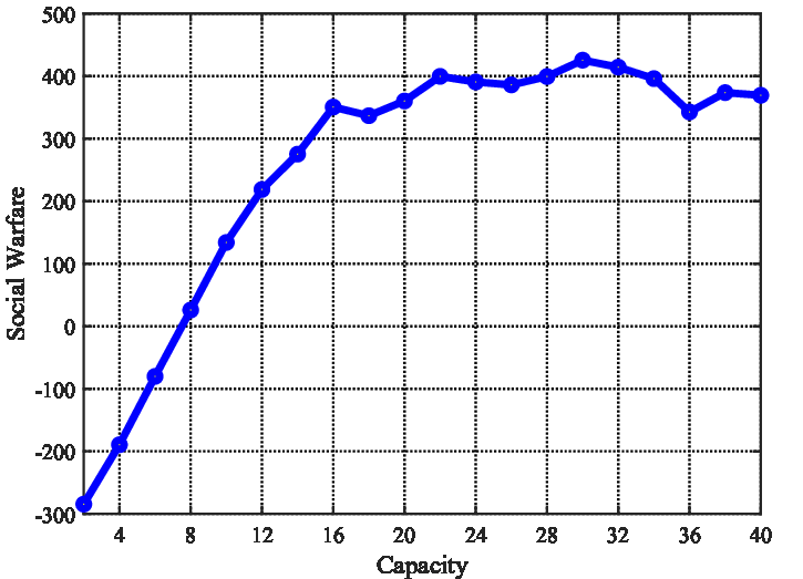

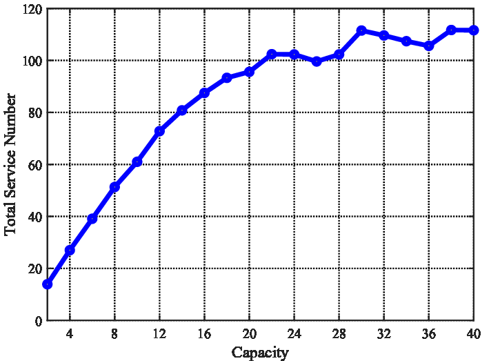


As the capacity of the charging piles and the arrival rate of EVs are critical to the operation of the charging station, we have also conducted sensitivity analysis to these factors by implementing policy . The result is shown in Fig. 8. From Fig. (a) to (c), it can be found that the social welfare, profit and the total service number of the charging station all increase with the capacity of the charging station increasing from 1 to 16. However, these curves appear to be steady when the capacity excesses 20. This is because the capacity of the charging station is enough to handle the current arrival rate of EVs in this case.
From Fig. (d) to (e), it can be seen that the social welfare firstly increases and then decreases with the increasing of the arrival rate. The optimal arrival rate for the charging station with capacity is about 14. This is because the increasing of the arrival rate will bring in the increasing service number of EVs as depicted in Fig. (f) which will improve the operation profit of the charging station as depicted in Fig. (d). However, when the arrival rate is too large, it will excess the service capacity of the charging station and incur the large QoS cost which makes the social welfare decreased. Similarly, due to the limited service capacity, the profit and the total service number also appear to be steady after the arrival rate excesses 20. These indicate it is necessary to investigate the EV traffic before planning the capacity of the charging station.
VI Conclusion
In this paper, the joint scheduling problem of pricing and charging control is studied to maximize the social welfare of the charging station considering the QoS and price fluctuation sensitivity of EVs. A two-phase online policy learning method is proposed to solve the formulated MDP model in the framework of event-based optimization. By utilizing performance difference theory, the performance improvement in each policy iteration is theoretically proved. Numerical results demonstrate the effectiveness of the proposed method and the operation improvement of the charging station.
Appendix A Proof of Lemma 1
Proof.
| (39) |
The first equation holds as the initial distribution is independent with policy or and the recursion is conducted. The third equation holds as there is . By using recursion for the last term in the third equation, Lemma 1 can be derived.
∎
Appendix B Proof of Theorem 1
Proof.
Based on Lemma 1, there is
| (40) |
Let . As and , there is
| (41) |
Substituting (41) into , we can derive
| (42) |
For (42), there is
| (43) |
Substituting (43) into (42) and using , there is
| (44) |
Substituting (44) into (40), we can derive
| (45) |
From (45), it can be seen that if the condition in theorem 1 is satisfied, there is . Furthermore, if there exists which the inequality strictly holds, there is . ∎
Appendix C Proof of Theorem 2
Proof.
We prove it by using contradiction. Suppose equation (29) does not hold for optimal policy . As the initial distribution is independent with the policies, we can at least find a action which has
| (46) |
where , and are the incurred values corresponding to . Therefore, a new policy can be constructed by the following mechanism,
| (47) |
Based on (45), we can derive . This means is not the optimal event-based scheduling policy which is contradictory. Thus, based on the above discussions, Theorem 2 is proven.
∎
References
- [1] A Guide for the Development of Electric Vehicle Charging Infrastructures (2015-2020) [online]. Available: http://www.nea.gov.cn/134828653_14478160183541n.pdf.
- [2] Z. Li and M. Ouyang, “The pricing of charging for electric vehicles in China-dilemma and solution,” Energy, vol. 36, no. 9, pp. 5765–5778, 2011.
- [3] H. S. Das, M. M. Rahman, S. Li, and C. Tan, “Electric vehicles standards, charging infrastructure, and impact on grid integration: A technological review,” Renewable and Sustainable Energy Reviews, vol. 120, p. 109618, 2020.
- [4] M. Moschella, P. Ferraro, E. Crisostomi, and R. Shorten, “Decentralized assignment of electric vehicles at charging stations based on personalized cost functions and distributed ledger technologies,” IEEE Internet Things J., vol. 8, no. 14, pp. 11 112–11 122, 2021.
- [5] J. Jin, L. Hao, Y. Xu, J. Wu, and Q.-S. Jia, “Joint scheduling of deferrable demand and storage with random supply and processing rate limits,” IEEE Trans. Autom. Control, vol. 66, no. 11, pp. 5506–5513, 2020.
- [6] Y. Cao, D. Li, Y. Zhang, and X. Chen, “Joint optimization of delay-tolerant autonomous electric vehicles charge scheduling and station battery degradation,” IEEE Internet Things J., vol. 7, no. 9, pp. 8590–8599, 2020.
- [7] A.-M. Koufakis, E. S. Rigas, N. Bassiliades, and S. D. Ramchurn, “Offline and online electric vehicle charging scheduling with V2V energy transfer,” IEEE Trans. Intell. Transp. Syst., vol. 21, no. 5, pp. 2128–2138, 2019.
- [8] Y. Yang, Q.-S. Jia, X. Guan, X. Zhang, Z. Qiu, and G. Deconinck, “Decentralized EV-based charging optimization with building integrated wind energy,” IEEE Trans. Autom. Sci. Eng., vol. 16, no. 3, pp. 1002–1017, 2018.
- [9] F. Zhang, Q. Yang, and D. An, “CDDPG: A deep-reinforcement-learning-based approach for electric vehicle charging control,” IEEE Internet Things J., vol. 8, no. 5, pp. 3075–3087, 2021.
- [10] V. S. Kasani, D. Tiwari, M. R. Khalghani, S. K. Solanki, and J. Solanki, “Optimal coordinated charging and routing scheme of electric vehicles in distribution grids: Real grid cases,” Sustainable Cities and Society, vol. 73, p. 103081, 2021.
- [11] C. R. Srivatsa, D. Rengarajan, and V. K. Tumuluru, “Modeling demand flexibility of electric vehicles,” in 2017 IEEE International Conference on Smart Grid Communications (SmartGridComm). IEEE, 2017, pp. 363–368.
- [12] L. Xia and S. Chen, “Dynamic pricing control for open queueing networks,” IEEE Trans. Autom. Control, vol. 63, no. 10, pp. 3290–3300, 2018.
- [13] Z. Zhao and C. K. Lee, “Dynamic pricing for EV charging stations: A deep reinforcement learning approach,” IEEE Trans. Transport. Electrific., 2021.
- [14] I. S. Bayram, M. Ismail, M. Abdallah, K. Qaraqe, and E. Serpedin, “A pricing-based load shifting framework for EV fast charging stations,” in 2014 IEEE International Conference on Smart Grid Communications (SmartGridComm). IEEE, 2014, pp. 680–685.
- [15] Y. Zhang, P. You, and L. Cai, “Optimal charging scheduling by pricing for EV charging station with dual charging modes,” IEEE Trans. Intell. Transp. Syst., vol. 20, no. 9, pp. 3386–3396, 2018.
- [16] A. Kapoor, V. Patel, A. Sharma, and A. Mohapatra, “Centralized and decentralized pricing strategies for optimal scheduling of electric vehicles,” IEEE Trans. Smart Grid, 2022.
- [17] T. Qian, C. Shao, X. Li, X. Wang, Z. Chen, and M. Shahidehpour, “Multi-agent deep reinforcement learning method for EV charging station game,” IEEE Trans. Power Syst., vol. 37, no. 3, pp. 1682–1694, 2021.
- [18] M. E. Kabir, C. Assi, M. H. K. Tushar, and J. Yan, “Optimal scheduling of EV charging at a solar power-based charging station,” IEEE Syst. J., vol. 14, no. 3, pp. 4221–4231, 2020.
- [19] M. L. Puterman, “Markov decision processes,” Handbooks in operations research and management science, vol. 2, pp. 331–434, 1990.
- [20] G. Li and X.-P. Zhang, “Modeling of plug-in hybrid electric vehicle charging demand in probabilistic power flow calculations,” IEEE Trans. Smart Grid, vol. 3, no. 1, pp. 492–499, 2012.
- [21] K. Jhala, B. Natarajan, A. Pahwa, and L. Erickson, “Real-time differential pricing scheme for active consumers with electric vehicles,” Electric Power Components and Systems, vol. 45, no. 14, pp. 1487–1497, 2017.
- [22] S. Sarkar and V. Ajjarapu, “MW resource assessment model for a hybrid energy conversion system with wind and solar resources,” IEEE Trans. Sustain. Energy, vol. 2, no. 4, pp. 383–391, 2011.
- [23] A. M. Foley, P. G. Leahy, A. Marvuglia, and E. J. McKeogh, “Current methods and advances in forecasting of wind power generation,” Renewable energy, vol. 37, no. 1, pp. 1–8, 2012.
- [24] M. Wytock, N. Moehle, and S. Boyd, “Dynamic energy management with scenario-based robust MPC,” in 2017 American Control Conference (ACC). IEEE, 2017, pp. 2042–2047.
- [25] L. Xia, “Risk-sensitive markov decision processes with combined metrics of mean and variance,” Production and Operations Management, vol. 29, no. 12, pp. 2808–2827, 2020.
- [26] X.-R. Cao, Stochastic Learning and Optimization: A Sensitivity-Based Approach. Springer, 2007.
- [27] NREL Solar Radiation Research Laboratory [online]. Available: https://midcdmz.nrel.gov/apps/sitehome.pl?site=BMS.
- [28] Q. Huang, Q.-S. Jia, and X. Guan, “A multi-timescale and bilevel coordination approach for matching uncertain wind supply with EV charging demand,” IEEE Trans. Autom. Sci. Eng., vol. 14, no. 2, pp. 694–704, 2017.
- [29] T. Long and Q.-S. Jia, “Joint optimization for coordinated charging control of commercial electric vehicles under distributed hydrogen energy supply,” IEEE Trans. Control Syst. Technol., vol. 30, no. 2, pp. 835–843, 2021.
- [30] Y. Xiang, J. Yang, X. Li, C. Gu, and S. Zhang, “Routing optimization of electric vehicles for charging with event-driven pricing strategy,” IEEE Trans. Autom. Sci. Eng., vol. 19, no. 1, pp. 7–20, 2021.