Infrared spectroscopy of the 2019 eruption of the recurrent nova V3890 Sgr: separation into equatorial and polar winds revealed2022Infrared spectroscopy of the 2019 eruption of the recurrent nova V3890 Sgr: separation into equatorial and polar winds revealed–References

A. Evans Thanks: E-mail:a.evans@keele.ac.uk Affiliation: Astrophysics Group, Lennard Jones Laboratory, Keele University, Keele, Staffordshire, ST5 5BG, UK T. R. Geballe Affiliation: Gemini Observatory/NSF’s NOIRLab, 670 N. Aohoku Place, Hilo, HI, 96720, USA C. E. Woodward Thanks: Visiting Astronomer at the Infrared Telescope Facility, which is operated by the University of Hawaii under contract 80HQTR19D0030 with the National Aeronautics and Space Administration. Affiliation: Minnesota Institute for Astrophysics, School of Physics & Astronomy, 116 Church Street SE, University of Minnesota,Minneapolis, MN 55455, USA D. P. K Banerjee Affiliation: Physical Research Laboratory, Navrangpura, Ahmedabad, Gujarat 380009, India R. D. Gehrz Affiliation: Minnesota Institute for Astrophysics, School of Physics & Astronomy, 116 Church Street SE, University of Minnesota,Minneapolis, MN 55455, USA S. Starrfield Affiliation: School of Earth and Space Exploration, Arizona State University, Box 871404, Tempe, AZ 85287-1404, USA M. Shahbandeh Affiliation: Department of Physics, Florida State University, 77 Chieftain Way, Tallahassee, FL 32306-4350, USA

Accepted XXX. Received YYY; in original form ZZZ

Abstract

We present infrared spectroscopy of the 2019 eruption of the recurrent nova V3890 Sgr, obtained over the period 5.1–46.3 days after the eruption. The spectrum of the red giant became more prominent as the flux declined, and by day 46.3 dominated the spectrum. Hydrogen and helium emission lines consisted of a narrow component superposed on a broad pedestal. The full width at half maximum of the narrow components declined with time $t$ as the eruption progressed, as ${t}^{-0.74}$ , whereas those of the broad components remained essentially constant. Conversely, the line fluxes of the narrow components of Pa $\beta$ remained roughly constant, while those of the broad components declined by a factor $\sim 30$ over a period of $\raisebox{-2.58334pt}{$\,\stackrel{{\scriptstyle\raisebox{-0.60275pt}{$\textstyle<$}}}{{\sim}}\,$}25$ days. The behaviour of the broad components is consistent with them arising in unencumbered fast-flowing ejecta perpendicular to the binary plane, in material that was ejected in a short $\sim 3.3$ -day burst. The narrow components arise in material that encounters the accumulated circumstellar material. The outburst spectra were rich in coronal lines. There were two coronal line phases, one that originated in gas ionised by supersoft X-ray source, the other in shocked gas. From the relative fluxes of silicon and sulphur coronal lines on day 23.4 – when the emitting gas was shocked – we deduce that the temperature of the coronal gas was $9.3\times 10^{5}$ K, and that the abundances are approximately solar.

Keywords:

shock waves — stars: individual: V3890 Sgr — novae, cataclysmic variables — infrared: stars

1 Introduction

Recurrent novae (RNe) are a subset of cataclysmic variables. They undergo thermonuclear runaway (TNR) eruptions but, unlike classical novae, their eruptions recur on timescales of $\sim 1-100$ years. The RNe can be sub-divided into those with short ( $\raisebox{-2.58334pt}{$\,\stackrel{{\scriptstyle\raisebox{-0.60275pt}{$\textstyle<$}}}{{\sim}}\,$}1$ day) and those with long ( $\sim 1$ yr) orbital periods (see Evans et al. 2008, for a review). As a consequence of the TNR, up to $10^{-6}$ M_⊙ of material, enhanced in heavy elements (particularly C, N, O, Mg, Al) is ejected at several 1000s of km s^-1 (Anupama 2008).

The long-orbital period RNe generally have red giant (RG) secondaries which, in common with field RGs, have winds. When a RN in a system with a RG secondary erupts, the ejected material collides with, and shocks, the RG wind, and a reverse shock is driven into the ejecta (Bode & Kahn 1985). This results in strong X-ray and radio emission, and coronal line emission in the UV, optical and infrared (IR). In addition, photoionisation is likely to play a part in the production of coronal line emission (Munari & Valisa 2022).

We present here a series of near IR (NIR) spectroscopic observations obtained during the 2019 eruption of the RN V3890 Sgr. Preliminary accounts have been given by Evans et al. 2019 and Woodward et al. 2019a; Woodward et al. 2019b. A description of various observations of V3890 Sgr obtained in quiescence is given by Kaminsky et al. 2022.

Refer to caption — Figure 1: $V$ -band light curve of V3890 Sgr; data from the AAVSO archive. Times of the observations reported here are indicated.

2 Properties of V3890 Sgr

2.1 The binary

V3890 Sgr underwent eruptions in 1962 and 1990 (Anupama 2008, e.g.). Its latest eruption was on 2019 Aug 27.87 (Pereira 2019, JD 2458723.37;). We take this to define our zero of time, $t=0$ . It has been reported to have an orbital period of $519.7\pm 0.3$ days and semi-major axis 362 R_⊙ (Schaefer 2009), but a more recent analysis, using extensive spectroscopic and photometric data (Mikołajewska et al. 2021), gives an orbital period of 747.6 days. Mikołajewska et al. 2021 give the mass of the white dwarf (WD) as $M_{\rm WD}\simeq 1.35\pm 0.13$ M_⊙, consistent with the view that the masses of the WD components in RNe are close to the Chandrasekhar limit (Starrfield et al. 1988; Anupama 2008).

The RG in V3890 Sgr has a mass $M_{\rm RG}\simeq 1.05\pm 0.11$ M_⊙, and a M5 III classification (Anupama 2008). This implies that, as in other examples of this sub-class of RNe, the material ejected during the TNR will encounter the RG wind, driving a shock into the wind, and a reverse shock into the ejecta (Bode & Kahn 1985). The orbital inclination is $\sim 67-69^{\circ}$ (Mikołajewska et al. 2021); we assume $68^{\circ}$ here.

The properties of V3890 Sgr in quiescence have been described in detail by Kaminsky et al. 2022. For the RG, they found small overabundances of both carbon and sodium relative to their solar values, while the abundances of oxygen and silicon are solar. The ¹²C/¹³C ratio was found to be $\sim 25$ , similar to that found in the RG components of other RNe.

Kaminsky et al. 2022 also found that a cool ( $\sim 400$ K) component is required to fit the continuum. This is clearly due to dust in the V3890 Sgr system. Silicate dust has been found in the environment of the RN RS Oph (Evans et al. 2007c; Woodward et al. 2008; Rushton et al. 2022), which is likely distributed in a torus around the binary; however there is no evidence for silicates in the environment of V3890 Sgr (Kaminsky et al. 2022).

Based on the pulsation of the RG, and on the assumption that the RG fills its Roche lobe, Mikołajewska et al. 2021 determined a distance of $D\simeq 9$ kpc.

2.2 Interstellar reddening

Munari & Walter 2019a measured the equivalent widths of interstellar Na i and K i absorption lines seen in high resolution optical spectra. They found $E(B-V)=0.56$ . They also noted that, as the intrinsic value of $(B-V)$ for novae 2 magnitudes from maximum is $(B-V)_{0}=0.02\pm 0.04$ (van den Bergh & Younger 1987), its early value of $(B-V)=0.67$ is consistent with $E(B-V)=0.67\pm 0.2$ . A thorough review of the reddening to V3890 Sgr was given by Page et al. 2020, who found values between $E(B-V)=0.48$ and 0.59. Kaminsky et al. 2022, in their anlysis of the IR spectrum, found that a value $E(B-V)=0.40$ gives the best fit. We take $E(B-V)=0.5$ here.

2.3 The 2019 eruption

The most recent RN eruption of V3890 Sgr was reported by Pereira 2019, and an optical spectrum was obtained within hours of outburst by Strader et al. 2019. Early NIR spectroscopy was reported by Rudy et al. 2019, who found that the emission lines were broad, with full widths at zero intensity (FWZI) of $\sim 10000$ km s^-1. Munari & Walter 2019b described the early optical emission lines as roughly triangular in profile, but containing a narrower ( $\sim 500$ km s^-1) component as the lines weakened; they also noted that the FWZI of H $\alpha$ was $\sim 8300$ km s^-1 on August 29 (close to visual maximum), and $\sim 7900$ km s^-1 on September 11 ( $\sim 14$ days after outburst), suggesting that little deceleration had taken place during that early interval. Munari & Walter 2019b also noted the presence of very sharp emission features, superimposed on the broad lines, which had disappeared by day 3.4. They suggested that these components arose in the flash-ionised RG wind, their disappearance being due to recombination, suggesting an electron density of $4\times 10^{7}$ cm^-3 in the wind. V3890 Sgr was detected in the radio (1.28 GHz) very early in the eruption by Nyamai et al. 2019.

Extensive X-ray observations of the 2019 eruption were described by Orio et al. 2020, Page et al. 2020 and Ness et al. 2022. Page et al. 2020 reported that the supersoft source (SSS) phase began around day 8.6, and persisted until day 26. They found that the temperature of the supersoft source rose to $T\sim 1.2\times 10^{6}$ K ( $kT\sim 100$ eV) between days 9.24 and 13.28, and that the spectrum steadily softened thereafter, up to day $\sim 26$ , when the effective blackbody temperature was $T\sim 4.6\times 10^{5}$ K ( $kT\simeq 40$ eV). The SSS phase in V3890 Sgr occurred much earlier in the eruption, and ended a much sooner, than was the case during either the 2006 or 2021 eruptions of the RN RS Oph (Orio et al. 2020; Page et al. 2020).

V3890 Sgr is one of the growing number of novae, both classical and recurrent, to have been detected in $\gamma$ -rays during eruption (Buson et al. 2019). In systems having RG secondaries, the observed high-energy $\gamma$ -rays probably arise as a result of collision between the RN ejecta and the RG wind, although in classical novae the most likely interpretation is shocks internal to the ejecta (see Chomiuk, Metzger & Shen 2021, for a thorough review; also Aydi et al. 2020).

The $V$ -band light curve from the AASVO archive¹¹ 1 https://www.aavso.org/ is shown in Fig. 1.

3 Observations

3.1 Gemini Observatory

NIR spectra of V3890 Sgr were obtained at both the Gemini South telescope (Eikenberry et al. 2012, with the facility spectrometer FLAMINGOS-2;) and the Frederick C. Gillett Gemini North telescope (Elias et al. 2006, with the facility spectrometer GNIRS;). Pertinent observational parameters are given in Table 1. All observations were obtained in the standard stare/nod-along-slit mode. Unlike most GNIRS cross-dispersed spectra, these GNIRS spectra were obtained with the $111\ell\,$ mm^-1 grating in order to obtain higher spectral resolution, and required three wavelength settings of that grating to cover the entire 0.8-2.5 $\,\mu$ m interval.

For the purpose of flux calibration and removal of telluric absorption lines, a nearby early A-type dwarf star was observed either immediately before or immediately after V3890 Sgr. The airmass difference between the science target and the telluric standard was in all cases $<0.13$ . Both V3890 Sgr and the telluric standards were observed with the slit oriented at the average parallactic angle.

Data reduction utilising both iraf²² 2 iraf is distributed by the National Optical Astronomy Observatories, which are operated by the Association of Universities for Research in Astronomy, Inc., under cooperative agreement with the National Science Foundation. (Tody 1986; Tody 1993) and figaro (Currie et al. 2014), employed standard procedures of spectrum extraction, spike removal, wavelength calibration (using spectra of argon arc lamps), removal of H i lines from the spectra of the standard star, cross correlating the spectra of V3890 Sgr and the telluric standard star and shifting the spectrum of the former to align it with the spectra of the standard star, and ratioing. The resolutions of the GNIRS spectra are roughly an order of magnitude higher than those of the FLAMINGOS-2 spectra. In the figures presented here the GNIRS spectra are sampled roughly an order of magnitude more finely than the FLAMINGOS-2 spectra (0.00010–0.00020 $\,\mu$ m versus 0.0010–0.0015 $\,\mu$ m).

3.2 IRTF

V3890 Sgr was observed with the NASA IRTF 3.2-m telescope on multiple epochs with the facility IR spectrograph SpeX (Rayner et al. 2003) in both SXD (short-crossed dispersed) and LXD (long-short crossed dispersed) modes, using slits matched to the seeing conditions, nodding the source at two positions (ABBA mode) in the slit set to the parallactic angle on the sky appropriate for the time of observations. Standard flat-field and calibration lamp (used to determine the wavelengths) spectra were obtained at the point position of the target. All spectra (V3890 Sgr and the associated telluric stars) were reduced using the IRTF IDL-based Spextool package (Cushing et al. 2004, version v4.1;) following standard IR techniques. Optimal point-source spectral extraction of the two-dimensional raw data frames was used. The aperture profiles were traced, and spectra extracted with parameters that typically used a Point Spread Function (PSF) radius and Aperture radius $=2\aas@@fstack{\prime\prime}2$ and $1\aas@@fstack{\prime\prime}0$ respectively. Background subtraction was enabled with the background sampling region starting at $2\aas@@fstack{\prime\prime}2$ (just outside the PSF radius) with a sampling width of $2\aas@@fstack{\prime\prime}0$ . The background was generated by a polynomial fit of degree $=1$ to data in the latter sampling region. The individual extracted spectra were then scaled (using order 3 for SXD and order 6 for LXD observations) and combined, after correcting the spectral shape of the orders, using a robust weighted mean technique with threshold value of 0.8 (Cushing et al. 2004, as described in). Flux calibration of the V3890 Sgr spectra was achieved using spectral type AOV telluric stars with known $B$ and $V$ magnitudes, following the methods described in Vacca et al. 2003. The deconvolution method was used for the SXD observations, using the hydrogen Pa $\gamma$ (1.09411 $\,\mu$ m) absorption feature in the continuum normalized spectra to construct the kernel relative to $\alpha$ Lyrae (Vega), with typical residuals having maximum deviations of $\raisebox{-2.58334pt}{$\,\stackrel{{\scriptstyle\raisebox{-0.60275pt}{$\textstyle<$}}}{{\sim}}\,$}3$ % and RMS deviation of $\raisebox{-2.58334pt}{$\,\stackrel{{\scriptstyle\raisebox{-0.60275pt}{$\textstyle<$}}}{{\sim}}\,$}1.6$ %. For the LXD observations, the convolution kernel was established from the arc lamp lines (Instrument Profile approach). Residual stellar H lines in the telluric spectra were removed through inspection and interpolation to produce telluric spectra containing only atmospheric absorption spectra. Lastly, each order was inspected to determine whether residual wavelength shifts were necessary to avoid introducing noise or artifacts when the V3890 Sgr spectra were divided by the telluric spectra.

Table 1 provides details of the Gemini and IRTF SpeX observations. The times of the IR spectroscopic observations are shown in Fig. 1.

4 Overview of the spectra

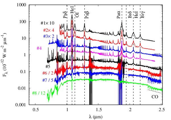
The entire dataset is displayed in Fig. 2. Some key features are summarised here, and are discussed in detail in the following subsections.

1.

The hydrogen and helium emission lines had narrow components, superposed on broad pedestals.
2.

By day 15.13, the first overtone CO bands, band-head at 2.29 $\,\mu$ m, were discernible in absorption; these must originate in the RG photosphere. They became progressively more prominent with time as the contribution from the ejected gas declined.
3.

Coronal lines were present from the earliest spectrum (day 5.11); unlike the H and He lines, they were narrow from the outset.
4.

On days 11.51 and 23.43 (when the spectra included wavelengths below 0.8 $\,\mu$ m), the Paschen (0.82 $\,\mu$ m) and Brackett (1.46 $\,\mu$ m) discontinuities were present and substantial, indicative of a relatively cool gas.

4.1 The continuum

As the continuum flux declined during the outbust, the contribution from the RG component became increasingly prominent. In order to facilitate the analysis of the nebular spectrum, the spectrum of the RG, obtained on 2020 May 20 (Kaminsky et al. 2022, day 266.66; described in), was subtracted from the data; there were no coronal lines on day 266.66. The spectrum from 2019 September 8 (day 11.51), dereddened and with the contribution from the RG removed, is shown in the left panel of Fig. 3; the continuum is fitted with a pure hydrogen nebular continuum at electron temperature $\sim 7000$ K and electron density $n_{e}=10^{7}$ cm^-3 (although the shape of the nebular continuum is not sensitive to $n_{e}$ ).

The right panel of this figure gives the same information, but for 2019 September 20 (day 23.43). In this case the fit, for a 6000 K nebular continuum, is not as good, but the large Paschen jump indicates a relatively low temperature gas. Such a low temperature is required to fit the Paschen and Brackett discontinuities at $\sim 0.82$ $\,\mu$ m and 1.46 $\,\mu$ m respectively.

As noted above, coronal lines, indicative of hot ( $\sim 10^{5}$ K), low density gas, are already present in the earliest spectrum. The cool (7000 K) gas observed on day 11.51 is unlikely to originate in the RG wind, flash-ionised by the ultraviolet pulse from the eruption, because the flash-ionised component had recombined by day 3.4 and had disappeared from the spectrum (Munari & Walter 2019b, see also Section 2.3). This flash-ionised component was not present in our first observation (day 5.11). However, with the spectral resolutions at our disposal at that time (see Table 1) our observations would not have detected such narrow features. The presence of substantial Paschen and Brackett discontinuities was recorded on day 11.81 of the 2006 eruption of the RN RS Oph (Evans et al. 2007a), but their explanation, in terms of flash-ionisation, may need reassessment.

Table 1: Log of infrared observations. “Day” is number of days since the start of the eruption on 2019 Aug 27.87 (JD 2458723.37).

UT Date	JD –	Day	Facility	Instrument	Airmass	Wavelength	Int.	Slit	Res’n	Telluric	Key to
YYYY-MM-DD.dd	2458000					range ( $\,\mu$ m)	time (s)	width (^′′)	$\lambda/\Delta\lambda$	standard	Fig. 2
2019-09-01.98	728.48	5.11	Gem-S	F-2 $J\!H$	1.03	0.89–2.40	8	0.36	200–1200	HIP97692	#1
				$H\!K$	1.02		8	0.36	300–1200	HIP97692	#1
2019-09-02.99	729.49	6.12	Gem-S	F-2 $J\!H$	1.03	0.89–2.40	8	0.18	200-1400	HD152602	#2
				$H\!K$	1.02		8	0.18	300–1500	HD152602	#2
2019-09-08.38	734.88	11.51	IRTF	SpeX	2.33	0.71–2.56	717		2000	HIP93901	#3
2019-09-12.00	738.50	15.13	Gem-S	F-2 $J\!H$	1.01	0.89–2.4	24	0.36	200–1200	HIP85607	#4
				F-2 $H\!K$	1.01		16	0.36	200–1200	HIP85607	#4
2019-09-20.30	746.80	23.43	IRTF	SpeX	1.74	0.69–2.56	20		2000	HIP93691	#5
2019-09-28.22	754.72	31.35	Gem-N	GNIRS	1.44	0.8–2.5	600	0.3	6000	HIP113673	#6
2019-10-13.22	769.72	46.35	Gem-N	GNIRS	1.57	0.8–2.5	600	0.3	6000	HIP94510	#7
2020-05-20.53	990.03	266.66	IRTF	SpeX	1.39	0.69–2.56	1618	0.8	750	HD168707	#8

4.2 Emission lines

4.2.1 H and He lines

Selected segments of the spectra, in the regions of particular emission lines, are shown in Fig. 4. It is evident from Figs 2 and 4 that some emission lines are broad on day 5.11, with narrow cores; the narrow components become progressively narrower with time. This is probably because ejected material is colliding with, and is decelerated by, the RG wind and any circumbinary material in the orbital plane that remains from previous eruptions and the common envelope phase. However, as discussed in Section 5, the picture is more complex than this.

The Pa $\alpha$ , Pa $\beta$ and Br $\gamma$ lines were isolated and uncomplicated by the presence of other features throughout our observations. We fitted these lines using two gaussian components, one for the narrow core, the other for the broad component. For some dates it was also possible to fit the He i lines at 1.083 $\,\mu$ m and 2.058 $\,\mu$ m. A typical fit is shown in the top panel of Fig. 5. We take the half width at half maximum (HWHM) of each component as an estimate of the velocity of the bulk of the ejecta, after deconvolving the instrumental resolution (also assumed to be gaussian).

The time-dependences of the HWHM velocities for the Pa $\alpha$ , Pa $\beta$ and Br $\gamma$ and He i lines, for both broad and narrow components, are shown in the middle panel of Fig. 5. There is a clear decline in the velocity widths of the narrow components, but little evidence of narrowing of the broad components. The expansion velocity as determined by the HWHMs of the narrow components of Pa $\beta$ (for which data exist for all seven dates) declines with time $t$ , roughly as $1840[\pm 490]\>\>t^{-0.75\pm 0.13}$ km s^-1, with $t$ in days. Furthermore, the narrow components of the He lines follow the trend shown by the H lines very well.

The behaviour of V3890 Sgr during its 2019 outburst closely resembled that of other RNe and nova systems containing a giant secondary. Deceleration of the ejecta is a common trait. This was seen in the eruptions of the RNe RS Oph (Das et al. 2006; Evans et al. 2007a; Pandey et al. 2022; Woodward et al. 2022) and V745 Sco (Banerjee et al. 2014), and in the symbiotic Nova Sco 2015 (Srivastava et al. 2015). It was also seen in the 2010 eruption of V407 Cyg, (Munari et al. 2011; Banerjee et al. 2014, their Fig. 3), a system that has a Mira secondary displaying $\sim 760$ d pulsations. Further, these systems (Srivastava et al. 2015, with the exception of Nova Sco 2015, which is probably too distant;) were detected as $\gamma$ -ray sources during outburst.

On the other hand, the expansion velocity of the material giving rise to the broad components seems relatively constant (Fig. 5); the mean HWHM velocity of the broad component of the H lines is $1740\pm 300$ km s^-1. The same behaviour is shown by the broad components of the He lines. For them the FWZIs of the broad components are $\sim 8000$ km s^-1, although for the He lines the FWZIs are less certain because of blends with other lines.

The time-dependence of the line fluxes $f$ , as typified by Pa $\beta$ , is shown in the bottom panel of Fig. 5. The fluxes from the narrow components decline relatively little over the course of our observations. The fluxes from the broad components, on the other hand, decline by a factor $\raisebox{-2.58334pt}{$\,\stackrel{{\scriptstyle\raisebox{-0.60275pt}{$\textstyle>$}}}{{\sim}}\,$}30$ over a period of $\raisebox{-2.58334pt}{$\,\stackrel{{\scriptstyle\raisebox{-0.60275pt}{$\textstyle<$}}}{{\sim}}\,$}25$ days, to such an extent that this component is hardly perceptible by day 46.35.

The general behaviour of the broad components may be understood in terms of a simple model in which the material is ejected into a cone over a brief time interval $\delta{t}$ , starting at $t=0$ , and disperses thereafter at constant velocity; we refer to this below as the “polar component”. For a given emission line (such as Pa $\beta$ ), the only variables in this model are the density of the emitting material, $N_{H}$ , and the electron density, $n_{e}$ , both of which we take to vary with distance $r$ as $r^{-2}$ . We assume that the electron temperature, mass-loss rate during ejection etc., remain constant. In these circumstances, the line flux $f$ follows a simple dependence on time:

	$\displaystyle f$	$\displaystyle\propto$	$\displaystyle\int_{R_{1}}^{R_{2}}\>\>n_{e}\>N_{H}\>\>r^{2}\>\>dr$		(1)
		$\displaystyle\propto$	$\displaystyle\frac{\delta{t}}{t(t-\delta{t})}\>\>.$		(1)

Here $R_{2}=Vt$ and $R_{1}=V(t-\delta{t})$ are the outer and inner radii of the ejecta respectively. A fit of this function to the data in the bottom panel of Fig. 5 shows a possible fit to the Pa $\beta$ data, with $\delta{t}=3.16\pm 0.48$ days. A similar result is obtained for Br $\gamma$ ( $\delta{t}=3.37\pm 0.41$ days). The fit for Pa $\alpha$ , with only four data points, is much poorer, $\delta{t}=1.71\pm 1.28$ days. The weighted mean for Pa $\beta$ and Br $\gamma$ gives $\delta{t}=3.3\pm 0.5$ days.

The behaviours of the H recombination and He i line profiles, together with those of a few other species, is further illustrated in Fig. 4. The top left panel of this figure shows the evolution of the spectrum at 2.0–2.2 $\,\mu$ m, which contains the He i 2.058 $\,\mu$ m and Br $\gamma$ lines. As the eruption progressed, the extrema of the broad components remained roughly at $\pm 4000$ km s^-1, while the narrow components became progressively narrower. The top right panel of this figure shows the evolution of the spectrum in the region of the He i 1.083 $\,\mu$ m and O i 1.129 $\,\mu$ m lines; again the widths of the broad pedestals in the He i and O i lines are constant. The middle and bottom left panels show the evolution of Pa $\beta$ and Pa $\alpha$ respectively; their behaviour is similar to that of Br $\gamma$ . The middle and bottom right panels show that the [Si x] 1.43 $\,\mu$ m and [S ix] 1.25 $\,\mu$ m coronal lines are narrow and essentially unresolved throughout, behaviour that is shared by all coronal lines.

4.2.2 Coronal lines

Coronal line fluxes.

The IR spectra contain a number of coronal lines (defined by Greenhouse et al. 1990, as emission lines “arising from ground-state fine-structure transitions in species with ionisation potential $>100$ eV”). These, together with their measured dereddened fluxes, are listed in Table 2; a representative spectrum (day 11.51) is shown in Fig. 6, which identifies H recombination and coronal lines. Many of these lines were present in the IR spectra of the 1985 and 2006 RN eruptions of RS Oph (Evans et al. 1988; Evans et al. 2007a; Evans et al. 2007b; Banerjee et al. 2009).

The most likely identification of the feature at 2.111 $\,\mu$ m (see Fig. 4) is He i (³S $-^{3}$ P), which is sometimes present in the NIR spectra of CNe (Naik, Banerjee & Ashok 2009; Raj et al. 2012; Raj et al. 2015, see, e.g.,). Its width is more comparable with those of other coronal lines (compare its width with that of He i 2.058 $\,\mu$ m in Fig. 4) suggesting that it too might be a coronal line, although it is weak so that any broad component might be lost in the noise. An alternative identification might be [Ca ix] (³P ${}_{2}-^{3}$ P₀) 2.111 $\,\mu$ m.

Fluxes of isolated coronal lines were mostly determined by fitting gaussians to the line profiles; where a coronal line is on the wing of a stronger feature, or where the continuum is evidently non-linear, a quadratic polynomial was fitted to the continuum, otherwise a linear continuum was used. In some cases the line sits on the wing of a much stronger line (e.g. [Al ix] 2.045 $\,\mu$ m on the blue wing of He i 2.058 $\,\mu$ m; see Fig. 4), making the line flux determination somewhat less reliable. In instances where the emission lines are crowded, the flux has been determined by trapezoidal integration between the FWZI points.

Temperature of the coronal gas.

The coronal line fluxes may be used to estimate the temperature of the gas in which the coronal lines originate, using

\frac{f(\mbox{A})}{f(\mbox{B})}=\frac{n\mbox{(A)}}{n\mbox{(B)}}\>\frac{\lambda_{\rm B}}{\lambda_{\rm A}}\>\frac{\Omega\mbox{(A)}}{\Omega\mbox{(B)}}\>\frac{g_{\rm B}}{g_{\rm A}}\>\>

(2)

(Greenhouse et al. 1990); here A and B are two ionic states from the same atomic species, the $f$ s are dereddened fluxes, the $n$ s are the number densities of the ions, the $\Omega$ s are effective collision strengths, and the $g$ values are the statistical weights of the lower levels. We take effective collision strengths from the IRON project³³ 3 http://cdsweb.u-strasbg.fr/tipbase/home.html (Hummer et al. 1993; Badnell et al. 2006). All ionisation fractions are from Arnaud & Rothenflug 1985, other than P xi, which is not listed in Arnaud & Rothenflug 1985; we take the value for $T=10^{6}$ K from Jain & Narain 1978 for P xi.

We assume an initial electron temperature $T$ , and calculate the effective collision strengths (which are $T$ -dependent); this gives a value for $n$ (A)/ $n$ (B). This in turn gives a new value of $T$ . The process is iterated until convergence occurs, which it does rather quickly. Where the Iron Project data do not extend to suffiently high temperatures (usually above $10^{5}$ K), we use the highest temperature available in the database (see Table 2 for these cases). Collision strengths and ionisation fractions are interpolated from tabulated values by fitting polynomials to the latter.

For two species we have spectral lines from three ionic states, namely Si ([Si vi], [Si vii] and [Si x]) and S ([S viii], [S ix] – two transitions – and [S xii]). We use the dereddended line fluxes for these species for day 23.43, when (a) there has been substantial deceleration of the ejecta (see Fig. 5) and (b) we expect photoionisation to be small towards the end of the SSS phase. Using Equation (2) for Si, we obtain $\log{T}$ values ( $T$ in K) of 5.69 ([Si vi] and [Si vii]) and 5.96 ([Si vii] and [Si x]). For S we get 5.95 ([S viii] and [S ix]) 6.17 ([S ix] and [S xii]) and 6.09 ([S viii] and [S xii]). Using these two species we find a mean $\log{T}=5.97\pm 0.11$ , or $T=9.3^{+2.7}_{-2.1}\times 10^{5}$ K on day 23.43. We assume $T=9.3\times 10^{5}$ K ( $kT=80$ eV) in what follows. The final values of $\Omega$ used are listed in Table 2.

Abundances in the coronal gas.

Further, by applying Equation (2), now with A and B representing different species (Greenhouse et al. 1990, see), we can determine the relative abundances of ionic species and, using the ionisation fraction as a function of temperature (Arnaud & Rothenflug 1985), the abundances of the elements themselves.

We have determined the abundances of each species X, by number, relative to Si, using ion pairs in the “matrix” of ions in Table 3. The abundance ratios as determined relative to [Si vii] and [Si x] are satisfyingly consistent for each ion — although there are differences between ions – while those determined using [Si vi] are consistently $\sim 1.4$ dex lower. For our present purposes, we take an overall mean, using all values for each species. These averaged abundance ratios, by number relative to Si, are given in the bottom row of Table 3.

The abundances are shown in Fig. 7, together with the corresponding solar (Asplund et al. 2021) and Arcturus (Peterson et al. 1993, K2III;) values, for comparison. Pavlenko et al. 2008; Pavlenko et al. 2020 and Kaminsky et al. 2022 have shown that the abundances of some of the light elements (specifically C, N, O, Si) differ from solar by less than one dex for the RG components of RNe, so the solar values provide a reasonable template. Also included in Fig. 7 are the expected abundance ratios for a TNR on the surface of a 1.35 M_⊙ WD, with 50:50 mixing of WD and accreted material (Starrfield et al. 2020); solar abundance has been assumed for Fe on the premise that Fe is not produced in a nova TNR.

Considering the crude nature of our abundance determination, the abundance ratios for V3890 Sgr are, with the exception of a deficiency of Al, surprisingly closer to the solar and Arcturus values than they are to the predictions of TNRs. However we should be mindful of the fact that V3890 Sgr, at $D=9$ kpc and close to the direction of the Galactic Centre (Galactic longitude $9\aas@@fstack{\circ}2$ ), is much closer to the Galactic Centre than either the Sun or Arcturus, and abundances in its RG component might also reflect metallicity gradients in the Milky Way (Maciel & Costa 2009, see, e.g..).

Coronal line “light curves”.

The time-dependences of the dereddened fluxes for some selected coronal lines (silicon, sulphur, calcium and aluminium) are shown in Fig. 8. There is a hint that some lines peak early in the eruption (e.g. [Al IX] 2.04 $\,\mu$ m), while others (e.g. [Si vii] 2.48 $\,\mu$ m, [Si x]) peak later ( $\,\stackrel{{\scriptstyle\raisebox{-0.60275pt}{$\textstyle>$}}}{{\sim}}\,$ 20 days).

Table 2: Coronal line fluxes. Fluxes, dereddened by

E(B-V)=0.5

, are in

10^{-17}

W m^-2; the flux for [P viii] (1.2784

\,\mu

m) includes contributions from both [P viii] and [Cr ix]. Upper limits are

3\sigma

. Wavelengths, from van Hoof (2018), are vacuum values. Ionisation potentials of the lower ionisation stage (IP; from the NIST Database^†) are in eV. Effective collision strengths

\Omega

are at

\log{T}\mbox{(K)}=5.97

unless otherwise specified; see text for details. Fluxes marked “*” denote lines in a crowded region of the spectrum, or lines that lie on the wing of a stronger line, and fluxes may not be completely reliable. A “—” denotes that the line was ouside the observed wavelength range.

Line identification			Day
ID	$\lambda$ ( $\mu$ m)	Transition $u-\ell$	IP	$\Omega$	5.11	6.12	11.51	15.13	23.43	31.35	46.35
[S xii]	0.7613	²P ${}_{3/2}-^{2}$ P_1/2	505	0.465	—	—	$95.8\pm 5.8$	—	$284.2\pm 3.0$	—	—
[Fe xi]	0.7894	²P ${}_{3/2}-^{2}$ P_1/2	262	0.887	—	—	$157.4\pm 5.3$	—	$408.6\pm 3.7$	—	—
[S ix]	0.9391	³P ${}_{0}-^{3}$ P₂	329	$0.264^{\ddagger}$	$294.6\pm 33.2^{*}$	$522\pm 20.5^{*}$	$261.9\pm 5.1$	$351.0\pm 26.6$	$64.6\pm 2.8$	$<6$	$4.9\pm 0.8^{*}$
[S viii]	0.9914	²P ${}_{1/2}-^{2}$ P_3/2	281	0.298	$<20$	$<46$	$211.1\pm 5.8$	$317.8\pm 16.1$	$82.4\pm 1.1$	$77.0\pm 0.7$	$28.7\pm 0.6$
[P xi]	1.0310	²P ${}_{3/2}-^{2}$ P_1/2	424	$0.543^{\ddagger}$	$191.8\pm 14.2^{*}$	$201.8\pm 24.1$	$82.9\pm 1.6$	$91.4\pm 8.0$	$21.4\pm 0.6$	$2.1\pm 0.2^{*}$	$<0.6$
[Fe xiii]	1.0750	³P ${}_{2}-^{3}$ P₁	331	2.638	$<290$	$<636$	$319.1\pm 11.9$	$<137$	$88.0\pm 4.6$	$18.2\pm 1.0^{*}$	$<1.9$
[S ix]	1.2523	³P ${}_{1}-^{3}$ P₂	329	$0.264^{\ddagger}$	$370.9\pm 46.1^{*}$	$350.5\pm 21.9^{*}$	$83.3\pm 2.8$	$202.2\pm 15.6$	$94.6\pm 1.1$	$46.2\pm 0.7$	$7.9\pm 0.8$
[P viii]	1.2784	²P ${}_{0}-^{2}$ P₂	264	—	$<19$	$<47$	$142.8\pm 4.6$	$<5.8$	$80.9\pm 3.4^{*}$	$19.9\pm 1.7^{*}$	$6.5\pm 0.9$
[Cr ix]	1.2786	³P ${}_{2}-^{3}$ P₁	185	—
[Si x]	1.4309	²P ${}_{3/2}-^{2}$ P_1/2	351	0.525	$<10$	$<17$	$34.4\pm 2.2$	$120.1\pm 13.8$	$127.8\pm 2.8$	$43.7\pm 2.3$	$<2$
[Si vi]	1.9650	²P ${}_{1/2}-^{2}$ P_3/2	167	0.380	$22.2\pm 1.9^{*}$	$12.6\pm 0.7^{*}$	$12.0\pm 1.7^{*}$	$<1.7$	$34.5\pm 2.2$	—	—
[Al ix]	2.0450^∗	²P ${}_{3/2}-^{2}$ P_1/2	285	0.604	$177.1\pm 18.0$	$207.2\pm 16.1$	$23.3\pm 1.4^{*}$	$16.7\pm 1.3^{*}$	$4.0\pm 0.6^{*}$	$<0.4$	$<0.6$
[Ca viii]	2.321	²P ${}^{o}_{3/2}-^{2}$ P ${}^{o}_{1/2}$	127	2.577	$15.5\pm 3.6^{*}$	$18.1\pm 2.6$	$21.3\pm 3.8$	$14.5\pm 1.1$	$8.7\pm 0.4$	$6.5\pm 0.7$	$<0.4$
[Si vii]	2.4833	³P ${}_{1}-^{3}$ P₂	205	0.695	—	—	$6.4\pm 0.6$	—	$33.3\pm 1.8$	$36.6\pm 1.6$	$27.8\pm 1.5$
^†https://www.nist.gov/.
^‡Value at $\log{T}\mbox{(K)}=5$ .

Table 3: Atomic abundances of X relative to Si,

\log

[

n

(X)/

n

(Si)], as determined from coronal lines. See text for details.

	[Al ix]	[P xi]	[S viii]	[S xi]	[S xi]	[S xii]	[Ca viii]	[Fe xi]	[Fe xiii]
$\lambda(\mbox{$\,\mu$m})=$	2.043	1.031	0.9914	0.9391	1.2523	0.7613	2.321	0.7894	1.0750
[Si vi]	–3.246	–2.834	–1.423	–1.397	–1.688	1.285	–1.305	–1.272	–0.412
[Si vii]	–1.914	–1.502	–0.091	–0.065	–0.356	2.617	0.027	0.060	0.920
[Si x]	–2.025	–1.613	–0.203	–0.177	–0.468	2.506	–0.085	–0.051	0.809
Adopted	Al	P	S				Ca	Fe
abundances	$-2.40\pm 0.43$	$-1.98\pm 0.43$	$0.05\pm 0.41$				$-0.46\pm 0.43$	$0.01\pm 0.32$

While we have no NIR data before day 5.11, spectra in the region of H $\alpha$ in the ARAS database⁴⁴ 4 http://www.astrosurf.com/aras/Aras_DataBase/DataBase.htm (Teyssier 2019) for $t\raisebox{-2.58334pt}{$\,\stackrel{{\scriptstyle\raisebox{-0.60275pt}{$\textstyle<$}}}{{\sim}}\,$}5$ days indicate that its narrow component was becoming narrower some time before our first NIR observation, possibly from outburst: clearly the ejecta were encountering significant resistance from near the time of outburst. Page et al. 2019a reported that the SSS phase of the 2019 eruption started on day 9.12, so that the gas would have been ionised by the early X-ray emission. The early coronal emission may therefore have arisen in a mix of shock-ionised and photoionised gas. The subsequent decline in the coronal line fluxes, with an $e$ -folding time of $\sim 15$ days (cf. Fig. 8), may correspond to the decline of the SSS phase; Page et al. 2019b; Page et al. 2020 report that the SSS phase in the 2019 eruption of V3890 Sgr had effectively ended by day 26. Fig. 8 (left and centre panels) suggests that the early-peaking coronal lines had also disappeared on this time-scale, suggesting that the coronal lines at the earlier times arose primarily in a photoionised gas, with shock ionisation also playing a role.

However, regarding the later ( $\raisebox{-2.58334pt}{$\,\stackrel{{\scriptstyle\raisebox{-0.60275pt}{$\textstyle>$}}}{{\sim}}\,$}23$ days) coronal emission, it is likely that the lines arise in a gas that is solely collisionally ionised and excited. As the ejecta encounter the RG wind, decelerate and are shocked, we expect a resurgence in the coronal line emission. We see in Fig. 8 that this results in the onset of emission in (for example) [Si x] 1.430 $\,\mu$ m, and the recovery of (for example) [Si vi] 1.96 $\,\mu$ m. It seems that the shock-origin for the coronal line emission sets in after $\sim 15-20$ days, just as the SSS-related coronal lines begin to fade.

Table 4: Critical electron density, determined as described in text, for coronal lines in Fig. 8.

ID	$\lambda$ ( $\mu$ m)	$A$ (s^-1)	$n_{\rm crit}$ (in cm^-3)
			at ${T}=9.3\times 10^{5}$ K
[S viii]	0.9914	18.64	$1.4\times 10^{10}$
[P xi]	1.0310	8.19	$6.8\times 10^{9}$
[Fe xiii]	1.0750	14.48	$3.1\times 10^{9}$
[Si x]	1.4309	3.15	$2.7\times 10^{9}$
[Si vi]	1.9650	2.38	$1.4\times 10^{9}$
[Al ix]	2.0450	1.07	$8.0\times 10^{8}$
[Ca viii]	2.321	0.70	$1.2\times 10^{8}$

There seems to be no obvious correlation of this behaviour with the IP values in Table 2. There is also no clear correlation with the critical electron density, $n_{\rm crit}$ , above which the upper level is collisionally, rather than radiatively, de-excited. The critical density at temperature $9.3\times 10^{5}$ K is (Osterbrock & Ferland 2006, see, e.g.,)

n_{\rm crit}=1.120\times 10^{8}\>\>\frac{A\>g_{2}}{\Omega(T)}

where $A$ is the Einstein coefficient for the transition, and $g_{2}$ is the statistical weight of the upper level. Einstein coefficients, where available, have been taken from van Hoof 2018. The resulting values of $n_{\rm crit}$ are given in Table 4. The high values of $n_{\rm crit}$ are a consequence of the high temperature of the coronal gas (as $n_{\rm crit}\propto{T}^{1/2}$ ). However the high values of critical density are consistent with the coronal lines arising in a relatively high density gas, such as that confined to the “equatorial” region, i.e. the region confined to the orbital plane (see below).

The fall and rise of some of the coronal line fluxes as the excitation mechanism switches from photionisation+shock, to shock only, is seen around day 15 in Fig. 8. A similar dip in coronal line fluxes, around day 70, was reported for the 2006 eruption of RS Oph by Evans et al. 2007b, who attributed this behaviour to the breakout of the ejecta from the RG wind. However the relative timescales of the SSS phase in V3890 Sgr and RS Oph ( $\sim 20$ days and $\sim 60$ days respectively) are similar to the times at which the “dips” occur in their respective coronal line light curves, suggesting that the duration of the SSS phase is a more likely explanation than breakout. This is consistent with a comparison of the distance travelled by the outer edge of the RG wind since the 1990 eruption to the distance travelled by the decelerating ejecta in the 2019 eruption. Kaminsky et al. 2022 suggest a wind velocity of 17 km s^-1 for the RG in V3890 Sgr; this is similar to that seen in field RGs (Wood, Müller & Harper 2016, see, e.g.,). The outer edge of the RG wind was therefore at $\sim 1.6\times 10^{15}$ cm at the time of our observations, while in time $t$ the 2019 ejecta will have travelled $\sim 8.6\times 10^{13}\,(t/5~\mbox{days})^{0.25}$ cm, assuming that the ejecta velocity varies as $t^{-0.75}$ (see Fig. 5). At the time of our last outburst observation ( $t=46.35$ days), this is $1.5\times 10^{14}$ cm. Clearly the ejecta were a long way from reaching the edge of the wind. The SSS hypothesis for the dips can obviously be tested when other RNe with RG secondaries erupt, in particular the 2021 eruption of RS Oph (Amorim, Muyllaert & Geary 2021) and the imminent eruption of T CrB (Luna et al. 2020).

5 Discussion

The usual paradigm for a nova eruption that occurs in a system containing a RG is that the ejected material collides with and collisionally shocks the RG wind. This is commonly evidenced by the appearance of coronal line emission in the optical and IR, X-ray emission and non-thermal radio emission, and the deceleration of the ejecta (see contributions in Evans et al. 2008, which reviews the 2006 eruption of RS Oph).

In the 2019 RN eruption of V3890 Sgr, all of these ingredients are present, but here we consider the implications of the NIR data. We summarise our findings as follows.

1.

On two dates (2019 September 8 and 20), there is evidence for a cool ( $\sim 7000$ K) gas that produced a free-free and free-bound continuum;
2.

the H recombination and He i lines consist of narrow components superposed on broad pedestals;
3.

the narrow components become progressively narrower in the H recombination lines, but the broad components remain stubbornly broad ( $\mbox{FWZI}\simeq 8000$ km s^-1) throughout our observations. Munari & Walter 2019b also noted that the width of the broad pedestals in optical emission lines had not changed during the first $\sim 15$ days. Both their data and ours imply that little deceleration of the material responsible for the broad pedestal emission occurred during this time;
4.

the narrow components of the H and He lines persist for the duration of our observations, although they weaken slightly with time;
5.

the fluxes in the broad components decline substantially over the period of our observations;
6.

coronal line emission is present from day 5.11; the coronal lines are narrow throughout the period of our observations;
7.

the temperature of the coronal gas, as determined from silicon and sulphur lines, is $\sim 9.3\times 10^{5}$ K;
8.

abundance ratios relative to Si of five elements, as determined from the coronal lines, are broadly similar to solar.

The progression of a nova eruption in a system containing a WD with an accretion disc, and a RG with a wind, has been considered in detail by Booth et al. 2016 in the context of the RN RS Oph, which superficially resembles V3890 Sgr in many ways. They find that, in the inter-eruption period, the interaction of the RG wind with the binary causes the majority of the wind to be confined to a circumbinary disc close to the orbital plane of the binary, and that the disc may be somewhat inclined to the binary plane (Theuns & Jorissen 1993, as discussed by). Observational evidence for enhanced density in the equatorial region for the case of RS Oph has been given by Ribeiro et al. 2009. Presumably the “old” silicate dust seen in the environment of RS Oph (Evans et al. 2007c; Woodward et al. 2008; Rushton et al. 2022), and the cool dust in V3890 Sgr (Kaminsky et al. 2022), reside in such a structure.

When the RN eruption occurs (see Booth et al. 2016, for details), the presence of the accretion disc restricts the flow in the orbital plane and imposes bipolar geometry on the nova ejecta: the ejected material escapes perpendicular to the orbital plane at $\sim 4000$ km s^-1. This is the same order of ejection velocity that we see in the broad emission line components in V3890 Sgr (the polar component). Our observed FWZI of $\sim 8000$ km s^-1 translates to an ejection velocity of $V=10700$ km s^-1 for an inclination of $68^{\circ}$ (Mikołajewska et al. 2021). Material ejected in the binary plane (the “equatorial” component) encounters the accumulated debris from the RG wind, previous eruptions and the common envelope phase.

As noted in subsection 4.2.2, there is evidence that the equatorial ejecta were encountering significant resistance from near the time of outburst. This behaviour is similar to that seen in the 2014 eruption of the RN V745 Sco, when the ejecta began sweeping up circumstellar material from the outset (Banerjee et al. 2014). The case of RS Oph is more complex, in that decelaration did not start until $\sim$ day 5 in the 2006 eruption (Das et al. 2006), but much earlier ( $\sim 3.9$ days) in its 2021 eruption (Pandey et al. 2022).

While we must be wary of extrapolating and of taking the fit too literally, it is intriguing that the $V\propto{t}^{-0.74}$ dependence for the velocities corresponding to the HWHM of the narrow components (see Section 4.2.1) extrapolates to $V\sim 10000$ km s^-1 at $t=0.1$ d, close to the velocity of the polar component. We might infer from this that all material was ejected at $\sim 10000$ km s^-1 in the TNR, ejecta in the polar direction moving without impediment, ejecta in the equatorial direction being severely decelerated from the outset, to $V\sim 100$ km s^-1.

The binary separation in V3890 Sgr is 2.2 AU (Mikołajewska et al. 2021). Material ejected in the 2019 eruption, decelerating as $V\propto{t}^{-0.75}$ , would reach the RG in $\sim 2$ hours. To a good approximation we may therefore suppose that the RN ejecta and the RG wind are co-centric, and that the ejecta run spherically symmetrically into the RG wind. We take the wind mass-loss from the RG to be $10^{-7}$ M_⊙ yr^-1 (Epsey & Crowley 2008; Banerjee et al. 2014, see, e.g.,), at velocity 17 km s^-1 (Kaminsky et al. 2022). The wind mass swept up by the ejecta in time $t$ , decelerating as discussed above, is $\simeq 1.2\times 10^{-7}\>{t}^{0.25}$ M_⊙, or $\simeq 1.8\times 10^{-7}$ M_⊙ in 5 days.

Under the assumptions that led to Equation (1), the ejected mass $M_{\rm ej}$ in the polar direction $M_{\rm ej}\propto\varpi{V}\delta{t}$ , where $\varpi$ is the solid angle of the cone into which the material is ejected. The ejected mass depends on $\varpi$ and $D$ as $M_{\rm ej}\propto\varpi^{1/2}D$ ; we assume that $D=9$ kpc (Mikołajewska et al. 2021). Using the dereddened fluxes of the broad components of the Pa $\alpha$ , Pa $\beta$ and Br $\gamma$ lines, we can estimate the ejected mass if we assume Case B, with an electron temperature of $T_{e}=2\times 10^{4}$ K. We take an arbitrary value of $\varpi$ corresponding to an apex angle for the conal ejection of $5^{\circ}$ , a highly collimated ejection.

The resuls are shown in Fig. 9, which includes the H mass in both polar components. Considering the simple

nature of the “model”, and the uncertainties in disentangling the broad and narrow line components, the individual masses are, with two exceptions (Br $\gamma$ on day 11.51 and Pa $\alpha$ on day 15.13), satisfyingly consistent. The mean value is $4.8[\pm 0.5]\times 10^{-6}$ M_⊙ and, as this is the mass in the form of H only, it represents a lower limit. The corresponding kinetic energy is $5.4\times 10^{38}$ J. While this is an estimate of the mass in the polar ejecta, we might suppose that the mass in the equatorial ejecta is not dissimilar, and if so, this mass is greater than our estimate of the RG wind mass swept up by the ejecta. Our estimated mass is similar to that ejected in other long-orbital period RNe (Anupama 2008, $3-4\times 10^{-6}$ M_⊙;).

With no complications arising from the RG wind, the line emission from the polar component should be determined by photoionisation only. For a TNR on the surface of a WD with mass close to the Chandrasekhar limit, the mass of helium in the ejecta is expected to be $\raisebox{-2.58334pt}{$\,\stackrel{{\scriptstyle\raisebox{-0.60275pt}{$\textstyle>$}}}{{\sim}}\,$}0.6$ times the mass of hydrogen depending on the degree of mixing of WD core and accreted material; see, e.g.,][]starrfield20, in contrast to the solar value of $\sim 0.3$ . To test this, we estimate the He/H ratio using the prescription of Krautter et al. 1984 which, for reasons discussed by those authors, gives a lower limit on $N(\mbox{He}^{+})/N(\mbox{H}^{+})$ . We use the measured fluxes in the broad components of the He i 2.058 $\,\mu$ m and Br $\gamma$ lines; the wavelengths are close enough that uncertainties in reddening and the need to deconvolve the lines from the instrumental resolution are not important. For days 5.11–31.34 (the broad components are too weak on day 46.35), we find a mean value for the lower limit on $N(\mbox{He}^{+})/N(\mbox{H}^{+})$ of $0.9\pm 0.2$ , implying that the He/H ratio by number is at least unity. This is an order of magnitude higher than the solar H/He ratio (Asplund et al. 2021, 0.082 by number;) and is consistent with the expectation for a TNR on a massive WD.

However the large wind mass close to the orbital plane, the accumulation of material lost by the RG wind over several orbits and possibly some material remaining from the common envelope phase, cause the nova ejecta to decelerate in this direction, to $\sim 100-200$ km s^-1; the ejecta sweep up the accumulated wind. In the $\sim 29$ years since the 1990 eruption, the accumulated wind in the circumstellar environment would have a mass $\sim 2.9\times 10^{-6}$ M_⊙ if the RG has mass-loss rate $\sim 10^{-7}$ M_⊙ yr^-1. This is comparable with the mass we estimated for the polar component (see above). Whereas the high velocity (polar) material is representative of material ejected in the TNR, the decelerated material, which encounters the RG wind, is expected to have a composition that is close to that of the RG (Booth et al. 2016). The coronal lines must arise in the equatorial component not yet reached by the RN ejecta, as they are persistently narrow and, unlike the H recombination lines, show no evidence of deceleration. The abundances we find in the coronal region (see Table 3), which must reside in the equatorial region, are approximatey solar; this is consistent with the scenario outlined by (Booth et al. 2016, but note our earlier caveat regarding Galactic abundance gradients).

The cool material, evidenced by the presence of the Paschen and Brackett discontinuities (see Fig. 3), presumably also lies in the equatorial region, but in a region where the electron density is $<4\times 10^{7}$ cm^-3 (Munari & Walter 2019b, see Section 2.3). Such a region is likely located on the outer edge of the equatorial region, where the electron density is likely to be lowest. This material was ionised during the eruption, but the 2019 ejecta have not yet reached it, and it has not recombined.

A cartoon of the likely circumbinary environment of V3890 Sgr during euption is shown in Fig. 10.

6 Conclusion

We have presented NIR spectroscopy of the 2019 eruption of the recurrent Nova V3890 Sgr. We conclude that

1.

the evolution of the emission lines suggest two distinct regions of ejected gas, one that results from the escape of ejecta at high velocity perpendicular to the binary plane (the polar component), and another that results from the interaction of both radiation from the nova and its high velocity ejecta with the accumulated wind of the RG and the detritus from previous RN eruptions (the equatorial component), resulting in rapid deceleration of the ejecta;
2.

the coronal line emission arises in the material that is confined to the equatorial component in the plane of the binary;
3.

the decline in the fluxes of the broad components of the H and He i emission lines suggests that the material was ejected in a brief pulse of about 3.3 days duration;
4.

the lower limit on the He/H ratio in the high-velocity material is consistent with the origin of this material in a TNR on the surface of a massive WD;
5.

the behaviour of the coronal line fluxes suggest that there were two coronal phases, an earlier phase when the coronal gas was both shock-ionised and photoionised, and a later phase when the coronal gas was truly coronal, in that the gas was collisionally heated and the transition upper levels were populated by electron impact;
6.

the temperature of the coronal gas was $9.3\times 10^{5}$ K;
7.

the metal abundances are consistent with solar and RG values, and inconsistent with those expected from a TNR on a massive WD.
8.

our data broadly support the scenario detailed by Booth et al. 2016.

Acknowledgements

We thank the referee for their comments which have helped to improve the paper.

The Gemini observations were made possible by awards of Director’s Discretionary Time for programmes GS-2019B-DD-102 and GN-2019B-DD-104. The international Gemini Observatory is a program of NSF’s NOIRLab, which is managed by the Association of Universities for Research in Astronomy (AURA) under a cooperative agreement with the National Science Foundation, on behalf of the Gemini Observatory partnership: the National Science Foundation (United States), National Research Council (Canada), Agencia Nacional de Investigación y Desarrollo (Chile), Ministerio de Ciencia, Tecnología e Innovación (Argentina), Ministério da Ciência, Tecnologia, Inovações e Comunicações (Brazil), and Korea Astronomy and Space Science Institute (Republic of Korea).

Additional data presented in this paper were obtained partly under IRTF programme 2020A-010. The Infrared Telescope Facility is operated by the University of Hawaii under contract 80HGTR19D0030 with the National Aeronautics and Space Administration.

CEW acknowledges partial support from NASA grant 80NSSC19K0868. DPKB is supported by a CSIR Emeritus Scientist grant-in-aid and is being hosted by the Physical Research Laboratory, Ahmedabad. RDG was supported by the United States Airforce.

We gratefully acknowledge the contributions of Terry Bolhsen and Umberto Sollecchia to the ARAS database.

We acknowledge with thanks the variable star observations from the AAVSO International Database contributed by observers worldwide and used in this research.

Data availability

The raw data in this paper are available from the Gemini Observatory Archive, https://archive.gemini.edu/, and from the IRTF archive, http://irtfweb.ifa.hawaii.edu/research/irtf_data_archive.php

References

Asplund et al. (2021) Asplund M., Amarsi A. M., Grevesse N., 2021, A&A, 653, A141
Amorim, Muyllaert & Geary (2021) Amorim A., Muyllaert E., Geary K., 2021, AAVSO Alert Notice 752
Anupama (2008) Anupama G. C., 2008, in RS Ophiuchi (2006) and the Recurrent Nova Phenomenon, Astronomical Society of the Pacific Conference Series, eds A. Evans, M. F. Bode, T. J. O’Brien, M. J. Darnley, vol. 401, p. 31, San Francisco
Arnaud & Rothenflug (1985) Arnaud M., Rothenflug R., 1985, A&AS, 60, 425
Aydi et al. (2020) Aydi E., et al., 2020, Nature Astronomy, 4, 776
Badnell et al. (2006) Badnell N. R., et al., 2006, in Planetary nebulae in our Galaxy and beyond, IAU Symposium 234, eds M. J. Barlow & R. H. Méndez, p. 211, Cambridge University Press, Cambridge
Banerjee et al. (2009) Banerjee D. P. K., Das R. K., Ashok N. M., 2009, MNRAS, 399, 357
Banerjee et al. (2014) Banerjee D. P. K., Joshi V., Venkataraman V., Ashok N. M., Marion G. H., Hsiao E. Y., Raj A., 2014, ApJ, 785, L11
Bode & Kahn (1985) Bode M. F., Kahn F. D., 1985, MNRAS, 217, 205
Booth et al. (2016) Booth R. A., Mohamed S., Podsiadlowski Ph., 2016, MNRAS, 457, 822
Buson et al. (2019) Buson S., Jean P., Cheung C. C., ATel 13114
Chomiuk, Metzger & Shen (2021) Chomiuk L., Metzger B. D., Shen K. J., 2021, ARA&A, 59, 391
Currie et al. (2014) Currie M. J., Berry D. S., Jenness, T., Gibb A. G., Bell G. S., Draper P. W., 2014, in Astronomical Data Analysis Software and Systems XXIII. eds N. Manset, P. Forshay, Astronomical Society of the Pacific Conference Series, vol. 485, p. 391, San Francisco
Cushing et al. (2004) Cushing M. C., Vacca W. D., Rayner J. T., 2004, PASP, 116, 362
Das et al. (2006) Das R., Banerjee D. P. K., Ashok N. M., 2006, ApJ, 653, L141
Eikenberry et al. (2012) Eikenberry S., et al., 2012, SPIE, 8446, 1
Elias et al. (2006) Elias J. H., Rodgers B., Joyce R. R., Lazo M., Doppmann G., Winge C., Rodriguez-Ardila A., in Ground-based and Airborne Instrumentation for Astronomy, eds. I. S. McLean and I. Masanori, 2006, SPIE, 6269, 36
Epsey & Crowley (2008) Espey B. R., Crowley C., 2008, in RS Ophiuchi (2006) and the Recurrent Nova Phenomenon, Astronomical Society of the Pacific Conference Series, eds A. Evans, M. F. Bode, T. J. O’Brien, M. J. Darnley, vol. 401, p. 166, San Francisco
Evans et al. (1988) Evans A. et al., 1988, MNRAS, 234, 755
Evans et al. (2007a) Evans A. et al., 2007a, MNRAS, 374, L1
Evans et al. (2007b) Evans A. et al., 2007b, ApJ, 663, L29
Evans et al. (2007c) Evans A. et al., 2007c, ApJ, 671, L157
Evans et al. (2008) Evans A., Bode M. F., O’Brien T. J., Darnley M. J., 2008, eds RS Ophiuchi (2006) and the Recurrent Nova Phenomenon, Astronomical Society of the Pacific Conference Series, vol. 401, San Francisco
Evans et al. (2019) Evans A., Banerjee D. P. K., Geballe T. R., Joshi V., Woodward C. E., Gehrz R. D., 2019, ATel 13088
Gehrz et al. (2007) Gehrz R. D., et al., 2007, Rev. Sci. Inst., 78, 011302
Greenhouse et al. (1990) Greenhouse M. A., Grasdalen G. L., Woodward C. E., Benson J., Gehrz R. D., Rosenthal E., Strutskie M. F., 1990, ApJ, 352, 307
Hummer et al. (1993) Hummer D. G., Berrington K. A., Eissner W., Anil K. P., Saraph H. E., Tully J. A., 1993, A&A, 279, 298
Jain & Narain (1978) Jain N. K., Narain U., 1978, A&AS, 31, 1
Kaminsky et al. (2022) Kaminsky B., et al., 2022, MNRAS, in press (arXiv:2207.14721)
Krautter et al. (1984) Krautter J., et al., 1984, A&A, 137, 307
Luna et al. (2020) Luna, G. J. M., Sokoloski, J. L., Mukai, K., Kuin, N. P. M., 2020, ApJ, 902, L14
Maciel & Costa (2009) Maciel W. J., Costa R. D. D., 2010, in Chemical Abundances in the Universe: Connecting the first stars to Planets, Proceedings of IAU Symposium 263, eds K. Cunha, M Spite, B. Barbuy, Cambridge University Press
Mikołajewska et al. (2021) Mikołajewska J., Iłkiewicz K., Gałan C., Monard B., Otulakowska-Hypka M., Sgara M. M., Udalski A., 2021, MNRAS, 504, 2122
Munari et al. (2011) Munari U., et al., 2011, MNRAS, 410, L52
Munari & Walter (2019a) Munari U, Walter F. M., 2019a, ATel 13069
Munari & Walter (2019b) Munari U, Walter F. M., 2019b, ATel 13099
Munari & Valisa (2022) Munari U., Valisa P., 2022, arXiv:2203.01378
Naik, Banerjee & Ashok (2009) Naik S., Banerjee D. P. K., Ashok N. M., 2009, MNRAS, 395, 1551
Ness et al. (2022) Ness J.-U., et al., 2022, A&A, 658, 169A
Nyamai et al. (2019) Nyamai M. M., Woudt P. A., Ribeiro V. A. R. M., Chomiuk L., 2019, ATel 13089
Osterbrock & Ferland (2006) Osterbrock D. E., Ferland G. J.,2006, Astrophysics of Gaseous Nebulae and Active Galactic Nuclei, second edition, University Science Books, Sausalito, California
Orio et al. (2020) Orio M., et al., 2020, ApJ, 895, 80
Page et al. (2019a) Page K. L., Beardmore A. P., Osborne J. P., Orio M., Sokolovsky K. V., Darnley M. J., 2019a, ATel 13084
Page et al. (2019b) Page K. L., Beardmore A. P., Osborne J. P., Kuin N. P. M., Ness J.-U., Orio M., Sokolovsky K. V., Starrfield S., 2019b, ATel 13137
Page et al. (2020) Page K. L., Kuin N. P. M., Beardmore A. P., Walter F. M., Osborne J. P., Markwardt C. B., Ness J.-U., Orio M., Sokolovsky K. V., 2020, MNRAS, 499, 4814
Pandey et al. (2022) Pandey R., Habtie G. R., Bandyopadhyay R., Das R., Teyssier F., Guarro Flo J., 2022, MNRAS, in press (arXiv:2207.10473)
Pavlenko et al. (2008) Pavlenko Y., Evans, A., Kerr T., Yakovina L., Woodward C. E., Lynch D., Rudy R., Pearson R. L., Russell R. W., 2008, A&A, 485, 541
Pavlenko et al. (2020) Pavlenko Y., Evans, A., Banerjee D. P. K., Geballe T. R., Munari U., Gehrz R. D., Woodward C. E., Starrfield S., 2020, MNRAS, 498, 4853
Pereira (2019) Pereira A., 2019, VSNET-ALERT 23506
Peterson et al. (1993) Peterson R. C., Dalle Ore C. M., Kurucz R. L., 1993, ApJ, 404, 333
Raj et al. (2012) Raj A., Ashok N. M., Banerjee D. P. K., Mundari U., Valisa P., Dallaporta S., 2012, MNRAS, 425, 2576
Raj et al. (2015) Raj A., Ashok N. M., Rudy R. J., Russell R. W., Lynch D. K., Woodward C. E., Sitko M., Day-Wilson A., Perry R. B., Kim S. C., Pak M., 2015, AJ, 149, 136
Rayner et al. (2003) Rayner J. T., Toomey D.W., Onaka P. M., Denault A. J., Stahlberger W. E.. Vacca W. D., Cushing M. C., Wang S., 2003, PASP, 115, 362
Ribeiro et al. (2009) Ribeiro, V. A. R. M., et al., 2009, ApJ, 703, 1955
Rudy et al. (2019) Rudy R., Subasavage J., Crawford Kirk., Gutierrez D., Russell R., Wiktorowicz S., 2019, ATel 13059
Rushton et al. (2022) Rushton M. T., Woodward C. E., Gehrz R. D., Evans A., Kaminsky B., Pavlenko Ya. V., Eyres S. P. S., 2022, MNRAS, submitted
Schaefer (2009) Schaefer B. E., 2009, ApJ, 697, 721
Srivastava et al. (2015) Srivastava M. K., Ashok N. M., Banerjee D. P. K., Sand D., 2015, MNRAS, 454, 1297
Starrfield et al. ( 1988) Starrfield S., Sparks W. M., Shaviv G., 1988, ApJ, 325, L35
Starrfield et al. (2020) Starrfield S., Bose M., Iliadis C., Hix W. R., Woodward C. E., Wagner R. M., 2020, ApJ, 895, 70
Strader et al. (2019) Strader J., et al., 2019, ATel 13047
Teyssier (2019) Teyssier F., 2019, Cont. Ast. Obs. Skalnaté Pleso, 49, 217
Theuns & Jorissen (1993) Theuns T., Jorissen A., 1993, MNRAS, 265, 946
Tody (1986) Tody D., 1986, in Proc. SPIE Instrumentation in Astronomy VI, ed. D.L. Crawford, 627, 733
Tody (1993) Tody D., in Astronomical Data Analysis Software and Systems II, Astronomical Society of the Pacific Conference Series, vol. 52, eds R. J. Hanisch, R. J. V. Brissenden, J. Barnes, 173, San Francisco
Vacca et al. (2003) Vacca W. D., Cushing M. C., Rayner J. T., PASP, 115, 390
van den Bergh & Younger (1987) van den Bergh S., Younger P. F., 1987, A&AS, 70, 125
van Hoof (2018) van Hoof P. A. M., 2018, Galaxies, 6, 63
Wood, Müller & Harper (2016) Wood B. E., Ml̈ler H.-R., Harper G. M., 2016, ApJ, 829, 74
Woodward et al. (2008) Woodward C. E. et al., 2008, in Evans A., Bode M. F., O’Brien T. J., Darnley M. J., eds, ASP Conf. Ser. Vol. 401, RS Ophiuchi (2006) and the Recurrent Nova Phenomenon. Astron. Soc. Pac., San Francisco, p. 260
Woodward et al. (2019a) Woodward C. E., Banerjee D. P. K., Evans A., Geballe T. R., Starrfield S., 2019a, ATel 13096
Woodward et al. (2019b) Woodward C. E., Banerjee D. P. K., Evans A., 2019b, ATel 13764
Woodward et al. (2022) Woodward C. E.,et al., 2022, in preparation