Electrical and Electronic Engineering \CSNameMartin Peter Neuenhofen \CSNameCover\CSname \CSNameTitleMartin Peter Neuenhofen \CSPositionPhD Student \CSDateAugust 11, 2026 \CSTitleQuadratic Integral Penalty Methods for Numerical Trajectory Optimization \CSSubTitleDissertation Thesis \CSKeyWordsNumerical Methods, Applied Mathematics, Optimal Control \CSCoverPictureimages/common/IC_LOGO.png \setThesisInfo
Chapter 0 Declaration of Originality
This work is – except for introduction and conclusion – a concatenation of other texts that the PhD student has written. The thesis consists of the following articles. They are listed in the order of appearance in the thesis:
- 1.
Martin P. Neuenhofen and Yuanbo Nie and Eric C. Kerrigan. Direct Quadrature Penalty Methods: Everywhere between Direct Integral Penalty and Direct Collocation Methods. Planned for publication.
- 2.
Martin P. Neuenhofen and Eric C. Kerrigan. A direct method for solving integral penalty transcription of optimal control problems. Proceedings of the IEEE Conference on Decision and Control 2020.
- 3.
Martin P. Neuenhofen and Eric C. Kerrigan. Dynamic Optimization with Convergence Guarantees. arXiv:1810.04059, 2018.
- 4.
Martin P. Neuenhofen and Eric C. Kerrigan. An integral penalty-barrier direct transcription method for optimal control. Proceedings of the IEEE Conference on Decision and Control 2020.
The majority of the thesis is based on the first item. The second and third item make Chapters 14–15. The fourth item is peer-reviewed published work that summarizes the method presented in the third item.
Yuanbo Nie has contributed to the numerical experiments in Section 4: We formulated the expressions of these problems so that they fit our format. He helped with generating interpolations from the interpolation data for the computed reference solutions in ICLOCS-II [98] that we used for validation. He also helped with the abstract and we had many valuable discussions on the design of figures and the line of presentation. This does not include the actual implementation of the experiments, of the solver, and the generation of data and figures.
In all items, Eric Kerrigan contributed to the theoretical analysis in the form of verification and modification of proofs, advice on the line of presentation, suitable formulations, and suggestions of references.
The independent contributions of the PhD student in all above listed items are the development and computational analysis, including the proof of convergence and of convergence rates, for all presented methods; further, the creation of figures and tables, design of examples, structure and organization of presentation, and most of the writing.
The following statement is provided by Imperial College London and confirmed by the student:
The work presented hereafter is based on research carried out by the author at the Imperial College London and it is all the author’s own work under supervisors’ supervision, except where otherwise acknowledged. Reuse of author’s own published works during the PhD degree program are also acknowledged according to publishers’ guidelines.
In reference to IEEE copyrighted material which is used with permission in this thesis, the IEEE does not endorse any of Imperial College London’s products or services. Internal or personal use of this material is permitted. If interested in reprinting/republishing IEEE copyrighted material for advertising or promotional purposes or for creating new collective works for resale or redistribution, please go to http://www.ieee.org/publications_standards/publications/rights/rights_link.html to learn how to obtain a License from RightsLink.
Martin Neuenhofen
London, March 2022
Chapter 1 Copyright Declaration
Students at Imperial College London must publish their PhD thesis under one of four possible licenses. The following states the license of this thesis and is a unique text defined by the selected license:
The copyright of this thesis rests with the author. Unless otherwise indicated, its contents are licensed under a Creative Commons Attribution-Non Commercial-No Derivatives 4.0 International Licence (CC BY-NC-ND). Link: https://creativecommons.org/licenses/by-nc-nd/4.0/
Under this licence, you may copy and redistribute the material in any medium or format on the condition that; you credit the author, do not use it for commercial purposes and do not distribute modified versions of the work.
When reusing or sharing this work, ensure you make the licence terms clear to others by naming the licence and linking to the licence text.
Please seek permission from the copyright holder for uses of this work that are not included in this licence or permitted under UK Copyright Law.
The below way of citation is suggested for this work:
Martin Peter Neuenhofen. Quadratic Integral Penalty Methods for Numerical Trajectory Optimization. PhD Thesis. Imperial College London. 2022.
Chapter 2 Abstract
This thesis presents new mathematical algorithms for the numerical solution of a mathematical problem class called dynamic optimization problems. These are mathematical optimization problems, i.e., problems in which numbers are sought that minimize an expression subject to obeying equality and inequality constraints. Dynamic optimization problems are distinct from non-dynamic problems in that the sought numbers may vary over one independent variable. This independent variable can be thought of as, e.g., time.
This thesis presents three methods, with emphasis on algorithms, convergence analysis, and computational demonstrations. The first method is a direct transcription method that is based on an integral quadratic penalty term. The purpose of this method is to avoid numerical artifacts such as ringing or erroneous/spurious solutions that may arise in direct collocation methods. The second method is a modified augmented Lagrangian method that leverages ideas from augmented Lagrangian methods for the solution of optimization problems with large quadratic penalty terms, such as they arise from the prior direct transcription method. Lastly, we present a direct transcription method with integral quadratic penalties and integral logarithmic barriers. All methods are motivated with applications and examples, analyzed with complete proofs for their convergence, and practically verified with numerical experiments.
Chapter 3 Acknowledgement
First and foremost, I would like to thank my supervisor, Prof. Eric Kerrigan, for the continuous support throughout this research program. The first time I got introduced to him was during my employment at Mercedes AMG Petronas Formula One. During my work there I came to notice that the methods we used to solve optimization problems did often fail to converge. I thus developed numerical methods and convergence analyses to fix these issues. When I searched for a PhD supervisor, I sent my drafts to Eric. After careful reading, he offered me supervision of my PhD thesis. He is a morally, fair, and very professional person. He never broke any agreements. He believed in my work from the start and gave me all possible freedom to do research on all kinds of methods related to optimal control. He was always interested and at most of the time had very good advice. I very much enjoyed working with him.
Special thanks go to Yuanbo Nie, who has introduced me to all the meta-subjects of PhD studies at Imperial. There are a lot of frustrating and unnecessary procedures. Yuanbo helped me a lot with the research, with the motivation, the work, the procedures, the LaTeX annoyances, the review frustrations, deep discussions, and also with practical help in uncountable instances. His wife and he offered me to stay at their apartment for three weeks and showed me the city when I came to visit London for the second time.
I would like to thank Chen Greif for everything he offered to me and for his huge financial support. I was introduced to Chen as a reviewer of a manuscript on next-generation Krylov methods. He was very interested and contributed eventually, and offered me a scholarship at UBC. As head of department, Chen was very busy at the time when I joined his group. Nonetheless, he was always very nice, supportive, went every extra mile that he could, and with Mstab we published a great piece of research.
Last but definitely not least, I thank my family. We build things together, share advice, go places, celebrate life, and enjoy every day.
Thanks to all of you!
Martin Neuenhofen
Mönchengladbach, March 2022
Chapter 4 Motivation of this Thesis and Overview of Presented Methods
As mentioned in the abstract, we present three numerical methods. All methods are either to directly transcribe dynamic optimization problems or to solve finite-dimensional nonlinear optimization problems that arise from the transcription.
Today, the state-of-the-art method for direct transcription is direct collocation. The motivation for the development and analysis of other methods stems from the fact that there are problems for which direct collocation fails to converge. Challenges are problems with singular arcs, with high-index differential-algebraic constraints, and problems with consistently over-determined constraints. This thesis is concerned with the development of numerical methods that can solve these problems in a black-box fashion reliably and efficiently to high accuracy.
In the following we give an abstract for each method. In Section 2 we explain how the thesis is structured and where each method is described in detail.
Method 1: Direct Quadrature Penalty Method
We present a quadrature penalty method as a competitive alternative to the popular method of direct collocation for solving optimal control problems with ordinary differential equations and differential-algebraic equations numerically.
There is consensus that direct collocation methods do not converge for some problems of practical interest. However, there is lack of practical means to assess the reasons behind these failures.
In this work, we aim to provide full transparency and accessibility to the numerical reasons behind the convergence of a generalization of direct collocation methods: quadrature penalty methods. A wealth of illustrated case studies, numerical experiments, and convergence theory demonstrates the practical benefits of quadrature penalty methods in terms of efficiency and robustness when compared to direct collocation.
To make the quadratic penalty method readily available for a wide audience, including readers who are new to optimal control, we include a full background to the origins, motivations, developments, and reasons behind the design of today’s optimal control methods. To improve accessibility, we refrained from sophisticated mathematics whenever it was possible to explain the same concept in a familiar but elaborate way. Familiarity with the following methods is sufficient: i) explicit Euler, ii) gradient-descent for local optimization, iii) Newton method for systems of equations, and iv) Gaussian quadrature.
Method 2: Modified Augmented Lagrangian Method
We present a numerical method for the minimization of constrained optimization problems where the objective is augmented with large quadratic penalties of inconsistent equality constraints. Such objectives arise from quadratic integral penalty methods for the direct transcription of optimal control problems.
The Augmented Lagrangian Method (ALM) has a number of advantages over the Quadratic Penalty Method (QPM). However, if the equality constraints are inconsistent, then ALM might not converge to a point that minimizes the bias of the objective and penalty term. Therefore, we present a modification of ALM that fits our purpose.
We prove convergence of the modified method and bound its local convergence rate by that of the unmodified method. Numerical experiments demonstrate that the modified ALM can minimize certain quadratic penalty-augmented functions faster than QPM, whereas the unmodified ALM converges to a minimizer of a significantly different problem.
Method 3: Penalty-Barrier Method with Quadratic Penalties and Logarithmic Barriers
We present a novel direct transcription method to solve optimization problems subject to nonlinear differential and inequality constraints.
We prove convergence of our numerical method under reasonably mild assumptions: boundedness and Lipschitz-continuity of the problem-defining functions. We do not require uniqueness, differentiability or constraint qualifications to hold and we avoid the use of Lagrange multipliers. Our approach differs fundamentally from well-known methods based on collocation; we follow a penalty-barrier approach, where we compute integral quadratic penalties on the equality path constraints and point constraints, and integral log-barriers on the inequality path constraints.
The resulting penalty-barrier functional can be minimized numerically using finite elements and penalty-barrier interior-point nonlinear programming solvers. Order of convergence results are derived, even if components of the solution are discontinuous.
Part 1 Introduction to Optimal Control
Chapter 5 Introduction to Optimal Control and Direct Transcription
In this first chapter, the concept of optimal control is introduced with three example applications. The first example considers the acceleration of an electric car. We will demonstrate how this optimal control problem can be solved by combining two familiar numerical methods. After laying out the general concepts, we describe in broad terms the contributions of this thesis. The subsequent Section 6 will introduce formal mathematical definitions.
1 From Optimization and Integration to Optimal Control
In the following two subsections, we recall two methods that are fundamental to applied mathematics. They will be combined later.
1 Explicit Euler Method
The explicit Euler method is attributed to Euler in 1768 [67]. This method solves initial value problems (IVPs) numerically. These take on the form: Given are initial values , a final time , and a flux-function . Find a function of that solves
| (1) |

Remark 1.1.
We use the symbol to abbreviate “for every” and to abbreviate “for almost every”. Other notations like “almost all (a.a.)” and “almost every (a.e.)” are commonly used for the same purpose in the context of differential equations in optimal control problems [86, 87, 64].
For example, the indicator function
is zero . Notice hence that
| (2) |
The reason for using in (1) is to accommodate cases where may be undefined at a countable infinite number of points (e.g., due to edges in ).
Figure 1 (a) shows an example of the explicit Euler method for the initial value problem
| (3) |
for various step-sizes .
2 Gradient-Descent Method
The gradient-descent method is a numerical method attributed to Cauchy in 1847 [32]. It solves optimization problems of the form: Given is an objective-function f. Find a local solution to
| (4) |
Remark 1.2.
We chose and f, which are unrelated, to keep standard notation of each sub-discipline and not opt for esoteric symbols. We write for the component of a vector x henceforth.
Figure 1 (b) shows an example of the gradient-descent method for minimizing
| (5) |
from the guess . A color-map visualizes values of f at coordinates . White lines illustrate contour lines of f. The method converges to the minimizer . We denote minimizers to optimization problems with a star superscript henceforth.
3 Integration + Optimization = Optimal Control
Optimal Control Problems are problems that combine the tasks of integrating functions and optimizing objectives. However, the optimization is not about finding optimal values of numbers. Instead, optimal shapes of functions must be found. Section 4 gives an example of what is meant by this.
Neither the explicit Euler method nor the gradient-descent method alone can optimize functions: The explicit Euler method can only integrate functions, while the gradient-descent method can only optimize numbers.
Figure 2 depicts the tasks of integration and optimization in a two-dimensional diagram. Traversal along the diagonal arrow requires one to integrate and optimize in a combined manner. For all practical purposes, optimal control problems are solved numerically with direct transcription. Direct transcription is a numerical method, just like explicit Euler method and gradient-descent method.
In the following subsections, we present and discuss an example of an optimal control problem: We formulate mathematically the application of an accelerating car as an optimal control problem. We then show how it can be solved with a numerical method. In-between, we give a brief subsection on terminology, notation, and symbols.
4 First Example of an Optimal Control Problem: Accelerating Car
Figure 3 illustrates an example of an optimal control problem. Suppose is the velocity of a vehicle at time . The car’s acceleration at time is modeled to depend on the throttle input and the present velocity , e.g. due to friction:
| (6) |
We wish to increase the car’s velocity from an initial value m/s to a final value m/s within a time limit of s. We wish to accelerate the vehicle such that the total wear and tear on energy storage, motors, and bearings is minimized. We model the wear as
| (7) |
There are many possible ways to transition from the initial velocity to the final velocity. Figure 3 illustrates three possible different ways in blue. Which way of transition leads to the least amount of wear and tear?
This question can be stated mathematically as
| (8) | ||||||
In this problem, we search functions for and such that passes through the initial and final values and satisfies the differential equation. The desired solution should minimize the wear from model (7).
5 Second Example: Maximizing Net Worth
We introduce a model from finance. This model is phrased into a mathematical problem. The problem is solved and gives an insight into finance.
Finance Model
Figure 4 presents a flow-chart from finance. Possession like solar panels or bitcoin farms produce revenue proportional to their value . This revenue is split into two purposes: A fraction is re-invested to buy more possession, whereas the rest is debited into savings . Net worth is the account balance of savings plus the resale price of the whole possession. At an initial time , we start with little possession and no savings: , . We seek to maximize net worth at the final time .
Mathematical Formulation
How should we design the split of revenue at each time in order to really become as rich as possible at ? Of course, initially we probably want to re-invest a lot whereas in the end it would not pay off anymore. But how do we arrive at an accurate answer?
The optimal profile of can be determined accurately by solving the following optimization problem:
| (9) |
Likewise, this can be posed as a minimization problem by minimizing the negative net worth.
Computational Solution
The solution to problem (9) are functions of time on the time-interval . Figure 5 presents the optimal solution: Final net worth is maximized when the revenue is fully re-invested into possession until and fully deposited into savings after . The optimal net worth is attained as .
6 Third Example: Economic Operation of a Commute Train
Suppose the following dynamic model for a commute train:
In these differential equations, is the position, the velocity, the acceleration, and the operational cost of the commute train. All physical units are SI units. Cost is in US Dollars. Cost is generated whenever the train moves and/or accelerates. For the purpose of this example, deceleration generates no cost, hence the max-expression in the last equation.
Figure 6 depicts the commute route: The train starts from Airport at time zero. At later time , the train is supposed to stop at Centre, which is at distance . For the example, we use and . As indicated in Figure 6, the conditions
are called boundary conditions. These just describe that the train stands still at both platforms, and that the train travels a distance of in time .
There are also bound constraints:
For the purpose of this example, these bounds arise from security policies and power limitations of the train.
We wish to find an optimal solution for such that the final cost is minimized. As depicted in Figure 6 in red and blue, multiple solutions for are possible that all yield the same traveled distance (area under the graph of ) and satisfy the boundary conditions.
The optimal solution is depicted in Figure 7: The optimal acceleration profile starts at the maximum value of and then steadily decays to zero. At about , the train will abruptly decelerate with maximum strength. Neither optimization alone nor integration alone could compute this solution.
7 Terminology of Optimization
In the next subsection, we show how problem (8) can be solved numerically. Before doing so, it is advantageous to agree on certain terms.
Classification
Figure 8 (a) shows an incomplete classification of optimization problems. These can be distinguished into finite and infinite optimization problems. Figure 1 (b) shows an example of a finite-dimensional optimization problem, because the solution is sought in the two-, i.e., finite-dimensional space . In contrast, optimal control problems belong into the class of infinite-dimensional optimization problems because continuous functions of cannot be represented as vectors in without loss of information.
Within the class of finite-dimensional optimization, problems can be distinguished into different categories: linear programming (LP), quadratic programming (QP), and nonlinear programming (NLP) [101]. This categorization is done because dedicated numerical solution software is available for problems of each category. NLP is the most general. Thus, numerical solution algorithms for NLP are also capable of solving LP and QP. Section 9 discusses NLP and numerical solution algorithms for NLP instances.
Sets
In contrast to format (4), most optimization problems feature constraints. Problem (8) is an example of a constrained optimization problem. Figure 8 (b) provides names of related sets: denotes the set of candidates. In problem (4), all candidates must live in , hence . In optimal control, the candidate spaces are so-called Sobolev spaces [109, 86, 87, 64], introduced later. When the optimization problem features constraints, we use the notation for the set of all candidates that are feasible w.r.t. satisfying the constraints. Among all feasible candidates, candidates that locally minimize the objective are called minimizers and are denoted with superscript .
8 Example of a Direct Transcription Method
In rare cases, optimal control problems can be solved with pen and paper. This is in fact the case for problem (8). The exact minimizer is , and . This minimizer is shown in the left of Figure 9. The figure also shows a numerical minimizer in the right. Engineers and other applied mathematicians are very interested in optimal control solutions because they provide critical insight into the efficient operation of assets. In the given example, the optimal control solution provides the counter-intuitive insight that it is most wear-economic to first decelerate before accelerating at a higher rate.
In practice, most optimal control problems can only be solved numerically. This section presents how (8) can be solved numerically for . The presentation uses a numerical method called direct transcription. In the example, the particular method used within the direct transcription is the explicit Euler method.
Direct methods are beneficial when numerical solutions must be found without detailed prior knowledge on what the solution might look like (in terms of, e.g., its shape or any properties). This thesis’ main focus is on direct methods. Section 1 will provide a literature review, where we also present and compare alternative methods for the numerical solution of optimal control problems.
Overview
Figure 8 shows the classes of optimal control in red and of NLP in blue. The key idea in direct transcription is to approximate the optimal control problem (8) with an NLP. The NLP in turn can be solved with methods like gradient-descent. The gradient-descent solution in turn can be used to construct . The following example guides the reader through this process. For the purpose of this example, we use the explicit Euler method. More sophisticated methods are used in practice. These are introduced later in Section 8.
Approximating the Optimal Control Problem with the Explicit Euler Method
The explicit Euler method uses a step-size for some to approximate differentials. Here, we do this for . The differentials in (6) are then approximated with the finite difference approximations
We use nodal approximations and . Inserting the finite difference approximations and nodal approximations, the differential equation (6) is replaced with
Transcription into NLP
Using the above explicit Euler approximation and left Riemann sums for the integral (7), the problem (8) reduces into:
| (10) |
This is an NLP (actually also a QP) with a solution . A local minimizer can be computed with numerical optimization algorithms. These algorithms are presented in Section 9. We denote the values in with .
Solving the Optimization Problem with the Gradient-Descent Method
For the purpose of this demonstration, we want to solve the NLP (10) with accessible methods. By eliminating the variables as follows,
we obtain an unconstrained minimization problem in the remaining two variables . Arranging these into a vector , the objective function becomes (5). Figure 1 (b) shows the minimization procedure of (5) with the gradient-descent method. Once we know , we can compute all the other values and construct the solution in the right of Figure 9. The interpolation of the values and is according to [16].
Accuracy of the Numerical Minimizer
Judging from Figure 9, the numerical solution is rather inaccurate. This is so because in this example is relatively large. We hope that for smaller values of the numerical solution converges to the exact minimizer . The following observation motivates this.
The exact control solution to problem 8 is , hence should solve the initial value problem (3) with . The explicit Euler solutions in Figure 1 (a) become more accurate as decreases. Likewise, the intention behind direct transcription is that the numerical minimizer converges to the exact minimizer as .
2 Scope of this Thesis
Figure 10 summarizes the previous section: Optimal control problems have exact minimizers that are often impractical to compute analytically. To find a solution numerically, we use a direct transcription method. This gives us an NLP, whose solution we can practically compute. The NLP’s solution gives us a numerical minimizer, which hopefully resembles the exact minimizer accurately. Different transcription methods result in different accuracies, and some methods do sometimes fail. Researchers and practitioners care about guarantees that can be given on the accuracy of a numerical solution for a given direct transcription method. Hence, this thesis is ultimately about the proposal of one particular direct transcription method that guarantees good accuracy under a large number of circumstances.
The direct transcription method that we propose is a quadrature penalty method, whereas the current state of the art in the literature are collocation methods. This is why the scope of this thesis is to great extent on these two classes of direct transcription methods: collocation, detailed in Section 8; and quadrature penalties, detailed in Section 11.
Quadrature penalty methods and collocation methods use different principles to accomplish the same tasks. These are:
- (a)
Approximating the time-dependent functions . As depicted in Figure 9, the explicit Euler method uses piecewise linear functions for and piecewise constant functions for .
- (b)
Relaxing the differential equations that were actually supposed to be satisfied . As apparent from the NLP (10) and Figure 1 (a), the explicit Euler solution is relaxed in the sense that it satisfies the differential equation only at the three points , , and . The relaxation is necessary because the solution to (6) is not piecewise linear.
Figure 11 illustrates the tasks of (a) approximation and (b) relaxation. The relaxation uses (i) a number of points in which the differential equations are solved to (ii) a certain accuracy. We will come back to this diagram in Section 2.
1 Direct Collocation Methods
Most direct transcription methods are generalizations of the explicit Euler method: They first (a) approximate with piecewise polynomial functions instead of piecewise linear functions. They then (b) relax the differential equations to be satisfied at only a (i) finite number of points in which they are solved (ii) exactly.
The principle of solving differential equations exactly at a finite number of points is called collocation. This principle is used in the explicit [86] and implicit Euler methods [87], in Runge-Kutta methods [64], in multi-step methods [62], in single [55] and multiple shooting [18] methods, and in a class of methods that is called collocation methods [16]. An overview of various numerical methods for optimal control is given in Section 7.
Today, direct collocation methods are considered as the state of the art for the numerical solution of optimal control problems. They will be presented in detail in Section 8.
As we discussed, the intention behind direct transcription methods is that the numerical minimizer converges to the exact minimizer as . Unfortunately, there are various practical kinds of optimal control problems for which the principle of collocation does not converge, including:
- •
nonlinear optimal control problems;
- •
consistently over-determined optimal control problems;
- •
singular-arc optimal control problems.
The lack of convergence in collocation methods for these classes of problems is analyzed in Section 10 and in Section 3.
2 Quadrature Penalty Methods
Coming back to Figure 11, all direct transcription methods (a) approximate with piecewise polynomial functions, just like collocation methods. However, there are different classes of direct transcription methods with respect to the (b) relaxation of the differential equations. These different classes can be located in a two-dimensional graph that answers the following two questions from Figure 11: (i) At how many points should we satisfy the differential equations? (ii) To which accuracy should we satisfy the differential equations at these points? The answers to these questions are opposed: Any approximation gives us a limited number of degrees of freedom. However, if we wish to satisfy the differential equations at more points then we cannot satisfy them as accurately at each of these points. Diagrams of meeting conflicting goals are called Pareto fronts.
Figure 12 presents this Pareto front for the above two questions: The choice of an (a) approximation determines a number of degrees of freedom. For example, the explicit Euler method with has degrees of freedom (DOF). As the red curve shows, we have to decide how to invest these DOF. We can either satisfy the differential equations at (i) only points but with (ii) exact accuracy — this is what collocation methods do. Alternatively, we can satisfy the differential equations at (i) many more points but to (ii) only moderate accuracy — this is what the so-called quadrature penalty methods do.
Quadrature penalty methods live between the extremes of collocation methods and integral penalty methods. Integral penalty methods are theoretical methods that satisfy the differential equations at (i) all points but to (ii) only low accuracy. Collocation methods and integral penalty methods are extreme in the sense that they live at the ends of the Pareto front: Collocation methods solve equations exactly, whereas integral penalty methods solve equations everywhere.
Collocation methods may fail to converge, and integral penalty methods may be impractical (e.g., when the exact solution to the integral cannot be found). The promise with quadrature penalty methods is that they meet both ends: they do converge and they are practical. When choosing many quadrature points, the quadrature penalty method approximates an integral penalty method. When choosing only a few quadrature points, the quadrature penalty method resembles a collocation method. This theoretically interesting because we can now understand the two extreme classes of methods as one class and unify their mathematical analysis. The practical interest for these methods is in their efficiency, as documented in Section 2, and in their reliability, as illustrated in Section 3. Convergence of high order (hence numerical efficiency) and under mild assumptions (hence numerical reliability) for this method is proven in Part 5.
3 Contributions
There are three main contributions in this thesis.
Quadrature Penalty Direct Transcription Method
Accessible Presentation
Our primary contribution is an accessible presentation of a reliable direct transcription method for the solution of a broad class of optimal control problems. This class are the direct quadrature penalty methods. As depicted in Figure 12, these methods generalize collocation methods and integral penalty methods. Part 3 presents these methods, illustrates their construction, and provides examples. We also discuss practical benefits in comparison to direct collocation methods. A wealth of numerical experiments demonstrate the practicality, performance, and robustness of quadrature penalty methods.
Convergence Analysis
Our second contribution is a complete convergence analysis for quadrature penalty methods. This analysis is given in Part 5 and is based on only three mild assumptions, given in Section 17. These are the mildest assumptions to date for a convergence proof of direct transcription methods, as confirmed through our extensive literature review.
Numerical Demonstration
Our third contribution is the detailed illustration and discussion of optimal control examples where popular direct transcription methods struggle. These examples are given in Section 10 and Section 3. These examples help motivate quadrature penalty methods and understand how they gain benefits in reliability. Prior to the presentation of quadrature penalty methods, we provide in Part 2 the necessary background on optimal control problems, on literature results, the context of different method classes and their relationships, in an accessible way.
Modified Augmented Lagrangian
The direct quadratic penalty transcriptions, that this thesis is focused on, result in NLP that have large quadratic penalty terms. In order to minimize these special NLP reliably in practice, a modification of the augmented Lagrangian method is proposed in Chapter 14 that works by solving a sequence of moderate penalty problems. Each of the moderate penalty problems can be solved reliably with general-purpose numerical optimization software. In contrast, solving one optimization problem with a large penalty term may cause general-purpose software to fail.
Integral Penalty-Barrier Direct Transcription Method
Large sparse NLPs are typically solved with interior-point methods (IPMs). More accurate transcription result in larger NLPs. It is often observed that larger NLPs require more computation cycles (i.e., iterations of the IPM) to converge. The penalty-barrier method seeks to avoid this effect: The penalty functional of the quadratic penalty direct transcription is replaced with a penalty-barrier functional. Minimizing said functional directly with a theoretical Newton/gradient-descent-type algorithm would result in a theoretical number of IPM iterations. Practical software on a transcription of finite dimensions may hopefully converge to this finite number of iterations as the dimension of the NLP grows. Again, as for the quadratic penalty method, the penalty-barrier method is presented in Chapter 15 with a full proof of convergence and order of convergence that work under still relatively mild assumptions.
Chapter 6 The Numerical Optimal Control Problem
This chapter provides a mathematically precise format for optimal control problems and introduces the necessary function spaces. Afterwards, in alignment with Figure 10, we discuss suitable measures for the assessment of the accuracy of a numerical solution.
1 Format of Optimal Control Problems
The electric vehicle problem (8) was just one very particular example of an optimal control problem. This section describes a more general format for optimal control problems. We first explain the solution format and then the problem format.
1 Solution Format
The solution of an optimal control problem consists of two functions . They are called states and controls, respectively. They must be of the following format:
The integers are the number of states and number of controls, respectively. In the electric vehicle problem (8), we had only state and control. This gives an informal description of the candidate space so that . A formal definition is in terms of Sobolev spaces and is given in Section 2.
Properties of States and Controls
In an optimal control problem, the state trajectories may have edges (in particular: an countable infinite number of discontinuities in the first derivative, as formalized in Section 4 below via the Lebesgue measure), but they must be continuous everywhere. This is so because differential equations like (6) demand that states evolve continuously over time. In contrast, controls may have discontinuities. This is to enable sudden control actions. An example of a discontinuous control is given in the lower right of Figure 9.
2 Problem Format
Many optimal control problems can be posed in Bolza form with fixed initial and final time [16]. In favour of less notation and ease of analysis, this thesis considers control problems in the following form:
| (1) |
Problem format (1) consists of four row-blocks, separated by vertical margins. In the first block, (1:M) states the objective . In the second block, (1:b) holds the boundary conditions . The third row-block consists of differential equations (1:f1) and algebraic equations (1:f2). The last block expresses left and right bound constraints on the states (1:y) and on the controls (1:u).
Remark 1.1.
The Bolza form has an additional so-called Lagrange term, i.e., an integral term in the objective. We saw such a term in example (8), where the objective was not only on but on an integral over . Such a term is missing in (1:M) for simplicity. A Lagrange term may be augmented to via the use of numerical quadrature (cf. first line in (10)) or via the techniques described in [16]. Algebraic inequality constraints can be embedded into (1:f2) and (1:u) via use of so-called slack controls [16].
Remark 1.2.
The differential and algebraic constraints may be violated at some points due to possible edges in and jumps in . This is formally taken care of by the notation. In contrast, for the bound constraints we can opt for the different notation . This helps avoiding ambiguity with the error measure in Section 3.
Remark 1.3.
There exist numerical algorithms and analyses for optimal control problems of more general formats. Some formats include partial differential equations, unknown parameters, and random variables in the boundary conditions or differential and algebraic constraints. The format of the problem can have dramatic impacts on the efficiency and thus suitable choice of a numerical algorithm. Therefor, any problem statement that cannot be expressed in terms of (1) is beyond the scope of this thesis.
Parameters and Functions in the Problem Format
In problem format (1), the numbers , are given parameters and
are given functions that must satisfy and , where is meant for each vector component.
3 Existence and Uniqueness of Solutions
Typical literature in numerical mathematics is structured in three steps: First, there is a section to present the problem statement. Second, there is a section verifying the “well-posedness” of the stated problem. Finally, a numerical method is presented and its convergence is analyzed. Well-posedness means that the solution to a problem changes mildly when the problem-defining functions and data are perturbed.
Basically, if a problem is not well-posed then it cannot be treated numerically in a meaningful way. This is because the numerical method, as well as the floating-point arithmetic, by itself induce perturbations that could radically change the solution unless the problem is well-posed. Nonetheless, the subject of well-posedness is generally a part of the convergence analysis: Namely, if a numerical method converges under particular assumptions then these assumptions must imply the well-posedness of the problem.
For the problem (1), which is the central problem statement of this thesis, it is clear that a solution might not exist. For instance, consider
Especially the theoretical realm of optimal control literature therefor considers rather restrictive problem statements, in order to enable the existence of clear conditions under which solutions exist and are well-posed. However, this has the disadvantage that practical optimal control problems are tedious to fit into the format of these literature’s problem statements.
As mentioned before, the analysis on well-posedness is implied in the analysis on convergence. For the quadrature penalty method proposed in this thesis, we obtain convergence to a local solution when:
- •
problem (1) has a global infimum;
- •
is feasible (needless to say);
- •
are point-wise local Hölder continuous in a neighborhood of ; and
- •
are bounded.
This does not mean that under these conditions is well-posed, i.e. would not change dramatically under small perturbations of . Rather, it means that the convergence measures (discussed below) of the numerical solution will not be affected significantly under small perturbations of –unless the four above conditions are not all met.
Essentially, in this thesis we wanted to avoid the discussion of well-posedness altogether because we consider it unhelpful for any problem in general (not limited to optimal control): The real world dictates problems in a natural problem statement. Numerics must make sense of these problem statements regardless; not by restricting them but by devising suitable metrics that are well-posed under all possible practical scenarios. The four bulleted conditions above are not a restriction but merely a characterization of what a practical scenario is. Therefor, no compromises had to be made in order to arrive at a problem statement that meets the two goals of generality and numerical practicality. The only peculiarity is now that we do not use the difference between exact and numerical solution as convergence metric because indeed this would usually result in ill-posedness. Instead, we are going to measure the optimality gap and a residual measure of the constraint violations.
2 Function Spaces in Optimal Control
In the terminology of Figure 8, the description of properties of states and controls from Section 1 above is an informal characterization of the candidate space . Formal definitions of candidate spaces in the literature use either Hölder spaces or the so-called Sobolev spaces. Sobolev spaces are based on Lebesgue spaces. For accessibility and because definitions of Lebesgue and Sobolev norms vary in the literature, this section reviews Hölder spaces, Lebesgue spaces, and Sobolev spaces. At the end we give a formal definition of the candidate space that we use in (1).
1 Hölder Spaces
Hölder spaces, Lebesgue spaces, and Sobolev spaces are function spaces; i.e., spaces that contain functions. We care in particular about functions of the form
for some dimension . The notation may be familiar to express that be times continuously differentiable.
A special form of continuity is Hölder continuity. We say is -Hölder continuous of constant on the interval if there is a constant such that
We use the typical notation for the space of functions whose first derivatives are -Hölder continuous on . The special case is the space of functions that are Lipschitz continuous, i.e. when . We use the short-hand for . In general, larger values of mean smoother functions. Hence, Hölder continuity is a milder condition than Lipschitz continuity.
2 Lebesgue Spaces
Hölder spaces are characterized by values of the function at individual points . Lebesgue spaces and Sobolev spaces are fundamentally different. They only depend on integral-norms over . We introduce Lebesgue spaces for as the spaces of all functions that are bounded in the norm
where for vectors . In the limit , the norms are
Like the supremum, the essential supremum always exists [43, p. 172]. The essential supremum induces the notion of essential boundedness. For instance, the indicator function is essentially bounded by zero. The space is a Hilbert space with scalar product
3 Sobolev Spaces
We introduce Sobolev spaces as the spaces of all times weakly differentiable functions that are bounded in the norm
| (3) |
Therein, denotes the weak derivative [23] of .11 1 For readers unfamiliar with a weak derivative, for simplicity, we can pretend that it is the conventional derivative and still follow the conceptual ideas. No emphasis on weak versus strong derivative is needed for the remainder of this thesis. We denote with the first weak derivative of . Hence, Sobolev spaces extend the idea of Lebesgue spaces to derivatives.
4 Candidate Space
In the Literature
Our Definition
The choice implies [23, Thm. 8.8], however may not be essentially bounded. This complicates the assumptions on the growth of , because may be unbounded at some points . To avoid this issue, we make use of the following space:
meaning that and are essentially bounded. We can hence formalize or space for equivalently in the following more insightful form:
| (4) |
In preparation for the convergence analysis, we also define the norm
| (5) |
where we mean the -norms for elements in by stacking into a vector:
| (6) |
3 Accuracy Measures
Figure 10 presents the flow chart of the conceptual idea behind direct transcription: By approximating the optimal control problem with an NLP, we obtain an approximate numerical minimizer to an exact minimizer . Accuracy measures can be used to quantify how good the numerical minimizer is in comparison to the exact one.
Connection between Optimality Conditions and Error Measures
A conventional analysis of optimal control would pose (1) in a format that is well-posed under some assumptions. The analysis would then establish a set of equations that are necessarily satisfied by every local solution of the optimal control problem. These equations are called Pontryagin equations (cf. Section 7). A numerical method is then devised to solve these equations approximately. The accuracy of this approximation is quantified and a bound of the deviation between numerical and exact solution is derived.
This thesis takes an entirely different approach. We do not use optimality conditions for the optimal control problem. Hence, we also do not care how the solution accuracy to such optimality conditions relates to the solution accuracy with respect to the optimal control problem. Furthermore, we do not use an error as a metric but instead we use a gap. This is explained and motivated in the following.
1 Motivation of Gap Measures
For optimization problems in general, we can use either of two metrics when measuring the accuracy of a numerical minimizer:
- 1.
Error: the distance between the numerical and the exact minimizer.
- 2.
Gap: the difference between the objective values of the numerical and the exact minimizer.
In optimization problems, and thus also in optimal control problems, the error does not necessarily converge. Hence, the gap may be the only suitable measure. To see why this is so, we provide some illustrations.
Illustration of Minimizers
Minimizers can be strict, non-strict, or unique [101, p. 13 & Lem 4.7 ii]. Figure 1 illustrates general challenges with minimizers of optimization problems: (a) Usually, problems can have several different exact minimizers. These can have different properties. (b) For instance, minimizers are called non-strict when the objective has a plateau. In the depicted example, all the points on the blue interval are local minimizers. (c) The existence of a unique minimizer can only be asserted under special circumstances, such as strict convexity. For instance, a sufficient condition for convexity in optimal control is called coercivity [86, 64, 65].
Most often, numerical algorithms can only compute local minimizers. As illustrated in (d), the numerical minimizer will converge to an exact local minimizer when that local minimizer is strict; thus the error converges. In contrast, in the case (e) of a non-strict minimizer, only the gap converges.
Consequences for Measurement
Because the error may not converge, we opted for the term accuracy measures instead of convergence measures. We will only consider the one-sided gap metric in (f): For a given exact minimizer under consideration, we measure the value of such that the objective of the numerical minimizer is bounded by . The possible locations of all sufficiently optimal numerical minimizers with respect to and are depicted in violet. Nothing prevents the numerical minimizer to converge to an even smaller local minimum than , which is beneficial.
2 Accuracy of Optimality
3 Accuracy of Feasibility to Equality Constraints
Consider the measure , that takes two functions and maps them onto a non-negative value:
| (8) |
where means the Euclidean norm of a vector in . Thus, quantifies: i) how well satisfy all the boundary constraints with at and ; ii) how well satisfy all the differential equations with and algebraic equations with for almost every , in the sense of . This is in analogy to how (2) is equivalent to .
A solution of problem (1) satisfies the constraints exactly because it is feasible. The numerical solution should hence be at least approximately feasible. Hence, the relation
| (9) |
should hold for a small equality residual .
4 Accuracy of Feasibility to Inequality Constraints
Of special importance to safety-critical applications, such as collision avoidance, is the property of numerical solutions to satisfy the left bounds and right bounds to high accuracy [112]. Hence, the relation
| (10a) | ||||||
| (10b) | ||||||
should hold for a small inequality residual .
5 Final Remarks
In Part 3 we present a direct transcription method for which we can prove that all three above measures converge to zero under mild assumptions. Part 5 provides the convergence proof.
A proof under mild assumptions is only possible because of the way how we formulate the convergence measures: We use the gap instead of the error. In addition to the gap, we use residual measures to assess the feasibility of a numerical minimizer.
Regarding these residuals, is an integral measure, whereas bounds violations in any point. This is a compromise for the numerics: We can, with very mild assumptions, assert that (10) is satisfiable numerically. In contrast, a property like would necessitate stronger assumptions on the smoothness of and of .
Part 2 Status Quo of Numerical Optimal Control
Chapter 7 Literature Review
Now that we have defined the problem statement and solution measures, it is natural to ask for the availability of numerical methods that are proven to converge for problem (1) under mild assumptions. A tabular literature overview of available convergence results is given at the end of this section. This will motivate our proof in Part 5, which works under favorable assumptions.
We first provide a broad overview of concepts and a historical survey of different developments. This is to answer two important questions: What is the state of research in the development of numerical algorithms for optimal control? Why do we only focus on direct transcription methods?
1 Overview of Concepts
Optimal control problems have several structural properties. Each property suggests a certain solution principle. Principles can be combined. To better explain these properties and principles, for the scope of this overview, we consider the following model problem:
| (1) |
In this model problem, we can suppose the control .
As far as known today, optimal control problems inherit four structural properties. These are depicted in Figure 1. We discuss them in order.
1 Optimal Subsolutions
Illustrated in Figure 1 (a), it holds that
because every minimizer of also minimizes the integrals over the sub-intervals and . Figure 1 (a) illustrates several non-optimal arcs in dashed besides the optimal arc in solid. The optimal arc over consists of the optimal arcs over and . Divide-and-conquer strategies use this property by dividing one optimal control problem into several smaller ones [107].
Example 1.1.
Direct transcription with the explicit Euler method divides into sub-intervals. is modelled piecewise linear on each sub-interval. The values at the red junction points are found by constrained optimization.
2 Overlapping Subproblems
As shown in Figure 1 (b), solutions of optimal control problems overlap. Figure 1 (b) plots the solutions of and . If we move both down just a little bit then their arcs lie on top of each other and match the solution of . Such strategy is used for example in the Schwarz predictor-corrector algorithm [91].
3 Greedy Substructures
Figure 1 (c) illustrates a greedy principle. Optimal substructures over an infinitesimal time-interval are straight lines. Hence, they can be computed greedily by forcing minimal. This provides a means for algorithms of the dynamic programming design paradigm: These propagate all optimal arcs backwards in time [12]. Afterwards, they select that particular arc that satisfies (dashed in the figure).
Example 1.2.
Bellman’s value function satisfies the hyperbolic end-value problem
| (2a) | ||||
| (2b) | ||||
The end-conditions are a function of and . In case there are no end-conditions , there holds that . This partial differential equation is known as the Hamilton-Jacobi-Bellman equation [12, 38]. Upon solution of , can be found as the solution of the initial value problem , .
4 Perturbability
Figure 1 (d) shows an optimal solution in black and perturbations of it in red. When a solution of is already optimal then the objective cannot be decreased any further via any of these perturbations. The red perturbation of shows an infinitesimal needle perturbation, whereas of shows a finite perturbation.
Direct Methods
Perturbations of finite length like result in so-called direct methods. These are methods that compose via splines such that an objective is minimized. Direct transcription with explicit Euler is an example of a direct method because the method constructs from piecewise linear functions such that is minimized.
Indirect Methods
By means of advanced calculus and limits of infinitely short needle perturbations, it is possible to derive the fact that exact minimizers of (1) must satisfy the following Euler-Lagrange conditions:
This is a so-called boundary value problem (BVP), in analogy to an initial value problem (IVP), because a differential equation must be solved subject to an initial and a final value. A generalization of the Euler-Lagrange conditions are the Pontryagin conditions [21]. These conditions also result in BVP. Methods that work via solving either of these boundary value problems are called indirect methods. Numerical methods for the solution of boundary value problems are introduced in Section 1.
Methods of perturbations are distinguished into direct methods and indirect methods because they reduce the optimal control problem into either of two different formats: direct methods result in NLP, whereas indirect methods result in boundary value problems.
5 Practicality
The greedy substructures face many technical issues, e.g., when cannot be determined uniquely or admits no classical solution [49]. Also, the back-propagation aspect and the spatial domain for in render dynamic programming algorithmic principles impractical due to memory-limitations when is large.
Predictor-corrector algorithms constitute a broad and blurry class. It is often not clear in which way to select a predictor-corrector algorithm in order to solve a particular optimal control problem.
Divide-and-conquer methods have been used widely in multiple direct/indirect shooting methods. These compute the subsolutions with direct/indirect methods and determine optimal values in a direct/indirect fashion. Mesh-refinement algorithms can also be considered as divide-and-conquer algorithms.
We now discuss methods based on perturbability. Indirect methods in this realm are unpopular for several reasons: Firstly, the boundary value problem resulting from the optimality conditions is often difficult to solve numerically [104, 62]. Numerical methods may diverge unless accurate initial guesses for the solution of the boundary value problem are given [25]. Secondly, for complicated optimal control problems it is difficult or impossible to determine the optimality conditions to begin with, hence there are problems which cannot be solved by indirect methods [20]. Even when possible, state-constrained problems require estimates of the intervals at which inequality constraints are active. Workarounds for state constraints, such as by saturation functions, have been proposed in [122]. Thirdly, for singular-arc problems, optimality conditions of higher order need to be used in order to determine a solution [83, Sec. 1.4]. Finally, the optimality conditions can have non-unique solutions.
In contrast, direct methods in this realm are very popular nowadays because they provide a direct means to discretizing the optimal control problem into an NLP. The NLP in turn can be solved with readily available solvers [101, 16, 80, 52]. However, this is the situation only since recently, as we depict in the following historical brief.
2 Historical Brief
Direct transcription methods are both a very recent and a very old class of methods. To understand how this is possible, we have to look into the historical developments of numerical methods for optimal control problems. Table 2 visualizes a timeline of different directions of development for numerical methods in optimal control. Revisiting these developments helps in assessing the maturity of each area and in identifying potential starting points for future research. We stress that the figure is not exhaustive and the depicted landmark contributions have certainly been inspired by fore-going research.
As the figure shows, computers existed only since 1930. However, today’s purpose of numerical methods and computers is that numerical methods solve mathematical problems on computers. This makes it fruitlessly debatable how early researchers would have intended their methods to be used on computers. For example, one could argue from Section 1 that direct collocation was invented by 1847: in Section 1 we construct a direct collocation method from the explicit Euler and the gradient-descent method. Both methods existed by 1847. However, the method of direct collocation is formally attributed to Hargraves et al. in 1987 [71]. We appreciate that attribution of contribution is an undecidable problem. Some methods, e.g., collocation and quadrature, are even so old that they cannot be clearly attributed to anyone.
The figure distinguishes several research directions: Analytic results mean equations and concepts that give analytic characterizations of solutions. Numerical methods provide formulas to generate approximations. Basic methods such as Newton’s method, quadrature, Euler’s method and gradient-descent form the origin of all modern numerical methods.
1 Euler-Lagrange Equations and Boundary Value Problems
The birth of optimal control is sometimes attributed to Johann Bernoulli for his discussion of the brachistochrone problem in 1697 [117]. In 1744, Euler identified the Euler-Lagrange differential equation as an analytic formula for how problems such as Bernoulli’s brachistochrone could be solved in a generic way [48]. The solution of optimal control problems via Euler-Lagrange equations results in boundary value problems.
Unlike initial value problems like (1), boundary value problems replace some conditions on the initial values with conditions on the end values . Methods for initial value problems are due to Euler in 1768 and have been generalized by Runge and Kutta in 1905. The first numerical method for boundary value problems however was the single shooting method. It was implemented on ENIAC, the first electrical and programmable computer, to calculate ballistic curves for the US military [89, 106]. Shooting methods work by iteratively guessing suitable initial values such that the solution of the initial value problem meets all conditions on the end values . The iterative scheme works via Newton’s method. This scheme was first described in the literature by Tifford only in 1951 [118].
As Figure 3 shows, there are multiple other ways than single shooting in terms of how Newton’s method can be combined with Runge-Kutta methods: (a) recalls the explicit Euler method as one example for a Runge-Kutta method. Euler’s method can be used to compute the blue nodes of from a given red initial value . (b) The single shooting method determines the initial value via Newton’s method such that a particular end condition is met. (c) Multiple shooting divides the interval into multiple (the figure shows two) sub-intervals. The initial values of each sub-interval are computed via Newton’s method such that the end-condition and finite-difference equations are satisfied. (d) Collocation methods include and solve all nodal values via Newton’s method.
The solutions of all three methods are algebraically equivalent, because they solve the exact same set of equations. However, methods with smaller propagation of perturbations of the red nodes (visualized in the figure in grey) result in better numerical conditioning and thus superior robustness for the Newton iteration. In addition, multiple shooting yields a smaller Newton system than collocation. Yet, multiple shooting may break when on any shooting interval the differential equation has a non-unique solution. This is so because any perturbation may result in switching between two different ODE solutions. Collocation avoids this issue altogether because the Newton system does not use ODE solutions but ODE residuals. Hence, collocation is preferred in practice.
Limitations of the Euler-Lagrange equations arise when the optimal control problem has inequality constraints. In this case, Pontryagin’s maximum principle (1956) provides a more general system of necessary conditions than the Euler-Lagrange equation [21]. In contrast to necessary conditions, the Bellman equation (1954) provides a constructional principle for globally optimal solutions to all local minimizers of optimal control problems [12]. The limitations to applying these analytic results for practical computations have been discussed in Section 5.
2 Direct Multiple Shooting and Direct Collocation
We saw in Figure 9 how the Euler method approximates with a piecewise linear function . However, doing so in the context of an optimization problem was first proposed by Ritz: To minimize, e.g., the functional
Ritz proposed approximating with a polynomial of fixed degree ; thus, resulting in a finite-dimensional optimization problem in for the coefficients of the polynomial. Implementations of Ritz methods typically use orthogonal polynomials due to numerical stability reasons; cf. (P1)–(P2) in [65]. Section 3 presents the the Ritz method on the above example in detail for .
Since Ritz, optimal control problems can be reduced directly into NLP. This is called direct transcription. Thus, optimization algorithms for NLP could be utilized for the numerical solution of optimal control problems. However, these algorithms had not been invented yet. Because of that, the NLP from Ritz method was solved via indirect methods, introduced by Galerkin. These are reviewed in Section 3. Modern direct solution methods for NLP are based on the equations derived by Karush in 1939 [79].
NLP can have equality and inequality constraints. The first widely used algorithm for inequality constrained optimization was Dantzig’s simplex method dated to 194711 1 There is no publication of Dantzig in this year. He invented it earlier and it was undisclosed in that year. [92]. This algorithm was only for LP, not NLP. The first method for NLP was the sequential quadratic programming (SQP) method by Wilson in 1963 [124]. However, at that time it would not have been possible to solve NLP that stem from the direct transcription of optimal control problems of relevant sizes. This is because these NLP are typically of large dimension, whereas computers at that time were slow and efficient data structures for large matrices did not yet exist.
It was only in 1971 that Wilkinson introduced the notion of a sparse matrix data structure. Collocation methods, multiple shooting methods, and Galerkin methods result in equation systems with large matrices that comprise mostly of zeros. A sparse matrix data structure avoids multiplications with and storage of zeros in these large matrices; thus making computations with the aforementioned methods possible at all. Algorithms with sparse matrix data structures emerged for solving equation systems and optimization problems of larger dimension; such as the Bunch-Kaufman factorization in 1977 [27] and a first practical interior-point algorithm by Karmarkar in 1984 [78].
The time at which optimization algorithms and practical optimization software became available explains why direct multiple shooting and direct collocation methods for solving optimal control problems entered the literature only by the 1980s. Before that point, it would have been difficult to propose such discretizations because there was no algorithm available to solve the resulting NLP. Due to similar reasons, as discussed along Figure 3, relating to conditioning and regularity, direct collocation is preferred over direct multiple shooting.
The constructional simplicity and practical success of direct collocation methods motivated research in convergence analysis. The first convergence proof for a direct collocation method is due to Malanowski et al. in 1997 [86]. They prove convergence of direct collocation with the explicit Euler method for optimal control problems where the dynamics are described as in (1), but with prescribed values for . This proof is very sophisticated as apparent from its assumptions. Earlier convergence results are available but consider significantly less general formats. More detailed convergence results are reviewed in Section 4.
3 Integral Penalty Methods and Quadrature Penalty Methods
Integral penalty methods were introduced by Courant in 1943 within a Rayleigh-Ritz method for partial differential equations [39]. This method uses quadratic penalization to enforce homogeneous Dirichlet boundary conditions. In the same manner that Galerkin generalized the necessary conditions of the Ritz method, as will be detailed in Section 3, Nitsche (1971) [100] generalized the necessary conditions of the quadratic integral penalty method.
Today, Nitsche methods are well-known and widely used for the solution [9] and optimal control [121, 119] of partial differential equations (PDE). For optimal control of nonlinear ordinary ODE and DAE however, collocation-type methods have been preferred over penalty-methods [15, 104]. This may be related to the fact that Runge-Kutta methods are usually preferred over finite element/volume/difference methods when solving ODE.
In [110], existence and convergence of solutions to two integral penalty functions of generic form were analyzed, but without a discretization scheme. Quadratic penalty functions of a less generic form, suiting optimal control problems with explicit initial conditions, were studied in [10]. The analysis focuses on the maximum principles that arise from the penalty function and their connection (under suitable assumptions on smoothness and uniqueness) to Pontryagin’s maximum principle, laying groundwork for an indirect solution to the penalty function. A numerical method is not proposed. In [74], the analysis is extended to inequality path constraints with a fractional barrier function. Using suitable smoothness and boundedness assumptions on the problem-defining functions, it is shown that the unconstrained minimizer converges from the interior to the original solution. As in [10], the analysis uses first-order necessary conditions. A numerical scheme on how to minimize the penalty functional is not presented. Limitations are in the smoothness assumptions.
In [42] the penalty function of [10] is used for problems with explicit initial conditions, linear dynamics and no path constraints. Under a local uniqueness assumption, convergence is proven for a direct discretization with piecewise constant functions for . The approach is extended in [63] to augmented Lagrangian methods with piecewise linear elements for the states. The analysis is mainly for linear-quadratic optimal control, which is used for approximately solving the inner iterations. The error in the outer iteration (augmented Lagrangian updates) contracts if the initial guess is sufficiently accurate [63, Lem. 3].
A convergence analysis for the use of integral penalties for equality constraints and integral geometric barriers for inequality constraints is given in [74]. This analysis shows that the constraint residuals and optimality gap of the penalty-barrier problem converge with respect to the original problem. The paper sketches how this analysis could be useful within a practical numerical scheme. The work in [97] provides a practical numerical method that uses quadratic penalties and logarithmic barriers instead of geometric barriers. Logarithmic barriers can be solved more efficiently in finite-dimensional optimization [52].
4 Final Remarks
Coming back to Table 2, research in numerical methods for optimal control accelerated with the advent and development of modern computers (beige). Today, it is possible to solve large sparse finite-dimensional optimization problems on affordable consumer computers.
Due to these developments, the most widely used class of numerical methods for solving optimal control problems today is direct transcription. The concepts of direct transcription methods are rooted in the Ritz method and orthogonal polynomials, highlighted in purple in Table 2. Among direct transcription methods, there are two classes of methods: Collocation methods are based on Runge-Kutta methods (red). Penalty methods are based on quadrature (blue).
3 Relation between Integral Penalty and Galerkin Methods
Integrals arise in integral penalty methods and in Galerkin methods. Both classes of methods are rarely used for the optimal control of ODE. Furthermore, Galerkin methods are a large class of non-trivial methods that may be unfamiliar to a wide readership in optimal control of ODE. Due to these reasons, this section reviews the conceptual ideas behind Galerkin methods and penalty methods in the context of optimal control problems. We use numerical examples to highlight differences and trade-offs between different methods.
A discussion of finite element methods, variational calculus, (bi-) linear forms, certain terminology and geometric interpretation (e.g., Galerkin-orthogonality) is avoided when possible because their introduction does not enhance accessibility. Interested readers are referred to [23, 119, 19].
Organization
Table 1 gives an organigram of three classes of methods for the solution of three classes of problems. The methods are: Ritz, Ritz-Galerkin, and weighted residual. The problems are: Unconstrained minimization, boundary value problems, and constrained minimization. Different methods may differ only in details, hence why the organigram works with three example problems that we crafted such that they are all mathematically equivalent. However, each numerical method yields a different numerical solution. In the following we explain each problem and method in the figure.
Equivalence of Problems
We show that the problems in Table 1 are equivalent. A suitable candidate space for the depicted unconstrained minimization problem is .
If we solve problem (4) in a subspace then the first-order necessary condition of optimality is:
In the above, is the directional derivative of f in the direction v. When then this is equivalent to .
Analogously, the necessary condition of optimality of
for any vector space is:
| (3) |
where
| (4) |
is the directional derivative.
The analytic solution of the unconstrained optimization problem and the boundary value problem is
Substituting , we see that the unconstrained and the constrained optimization problem in Table 1 are related. In the following, we discuss numerical methods for solving each of the three depicted problem classes in the figure.
1 Unconstrained Minimization
Ritz Method
In order to solve unconstrained optimization problems with readily available methods, Ritz (1909) proposed to replace the infinite-dimensional candidate space with a finite-dimensional ansatz space22 2 We use the terms candidate space and ansatz space to avoid the use of the term search space, which could be confused with either of the two. A candidate space is a property of the problem statement. An ansatz space is a property of a numerical method.. For the purpose of this example, we choose the space of cubic polynomials . This is a discretization of dimension . This gives us the ansatz
| (5) | ||||
which we can insert into the integral expression of :
The Ritz method is the minimization of in the ansatz space; hence an NLP of the form (5). We can compute a minimizer for with the gradient-descent method, resulting in . Thus, the solution of the Ritz method is
This is a very accurate numerical solution. Figure 4 shows the error between the Ritz solution and in blue. We see that the error is smaller than everywhere.
Ritz-Galerkin Method
The Ritz method minimizes directly in the ansatz space. Recalling the necessary optimality condition (3), solutions of the Ritz method must satisfy
| (6) |
The solution of equations of this form was first proposed by Galerkin in 1915 [54]. For the aforementioned reasons, this yields the same solution as the Ritz method; hence why this method is called the Ritz-Galerkin method. Inserting (4) and as stated in Table 1 under Weak Form, we may write (6) as
| (7) |
We explain later why it is called the Weak Form. Using the representations (5) and
the condition (7) can be represented as
| (8) |
which can be solved as linear system for x. The entries in the matrix and right-hand side vector are and , . When is nonlinear in then is nonlinear in x and one must resort to, e.g., Newton iterations.
2 Boundary Value Problems
The above formulation is called weak form because it only assumes that . In contrast, if we make the strong assumption that is well-defined then the directional derivative from (4) can be re-expressed by virtue of partial integration:
Apart from the partial integration, in the directional derivative we also replaced the symbol of a direction with a so-called test function in a suitable test space . If we want to satisfy independent of any values for , , and , then we must find that satisfies the boundary value problem in Table 1.
Weighted Residual Method
We can satisfy
by choosing the new approach
for . Thus, satisfies the boundary conditions naturally. We can then solve the boundary value problem numerically as depicted in Table 1 under Strong Form.
There are three common weighted residual methods. The Bubnov-Galerkin method uses , i.e. the same test space as ansatz space. The Galerkin Least-Squares method uses a space that depends on the differential equation at hand: The method forms the least-squares functional
The method then applies the Ritz-Galerkin method to the minimization of that functional. This results in the following equation:
Thus, the Galerkin Least-Squares method can be written in the same way as the Bubnov-Galerkin method in Table 1 by selecting . The Galerkin Least-Squares method always yields a symmetric linear system. In contrast, Petrov-Galerkin methods are methods where the system matrix is non-symmetric and . Lastly, there are collocation methods. These read: Find , such that
where is set of points; i.e., two points in our example.
Numerical Comparison
We now compare the methods of Ritz-Galerkin, Bubnov-Galerkin, Galerkin Least-Squares, and Collocation with numerically. Figure 4 plots the error of each method. Due to symmetry and overlap, the error vanishes at and at some other method-specific points. The figure confirms that indeed each method yields a different solution.
3 Constrained Minimization
Optimal control problems use mixed formulations [19]. These are problems that combine a Ritz or Ritz-Galerkin method for the ansatz space with a weighted residual method for the constraints. Table 1 color-indicates both portions of the problem. In the figure, is a place-holder for an arbitrary weighted residual method. There are at least three ways for numerically solving the constrained minimization problem.
Lagrange Method
Using a Lagrange multiplier , we can apply a Ritz method or Ritz-Galerkin method to find the stationary point of the Lagrangian functional. The directional derivatives are:
Setting them to zero for a given test space yields a symmetric linear system, just like (8). We introduce these systems in the next paragraph. However, the matrix of this linear system is often singular unless is chosen in a special way such that the Ladyzhenskaya–Babuska–Brezzi condition is satisfied [19]. Finding a suitable requires sophisticated functional analysis for each constrained minimization problem at hand.
Regularized Lagrange Method
It thus makes sense to regularize the Lagrangian via the purple term with a small regularization parameter . In the symmetric linear system this will yield a negative definite block in the lower right, shown in purple in Table 1 under Regularized Lagrangian, Ritz-Galerkin. This may help regularizing the linear system. On the flip-side, the magnitude of alters the numerical solution of . Also, the Lagrangian method necessitates a basis representation for ; cf. in (8). We will show different system matrices below in the numerical comparison. Equation systems of the above form have been proposed by Nitsche in 1971 [100].
Quadratic Penalty Method
Because of the hassle with a suitable basis for and regularization, it seems attractive to use an alternative method altogether. The quadratic penalty method (Courant, 1943) is such an alternative. The method works by forming
and solving the unconstrained minimization problem with a direct method (e.g., conjugate gradients). In the above, is a small penalty parameter.
Since the Ritz and the Ritz-Galerkin method both generate the same solution, we can now use the latter to derive an equation system. The directional derivatives are:
Hence, the Ritz-Galerkin method reads: Find , such that
| (9) |
If then we can substitute in the Ritz-Galerkin method for the regularized Lagrangian. Thus, under this special choice of , the quadratic penalty method and the regularized Lagrangian method are equivalent.
4 Comparison: Galerkin Least-Squares Method vs Quadratic Penalty Method
The quadratic penalty method may be confused with the Galerkin Least-Squares method. However, both methods are unrelated: The Galerkin Least-Squares method is a non-trivial choice of , whereas the quadratic penalty method is a method where is absent.
In the given example, because we suppose that the constraint uniquely determines from given values of , the Galerkin Least-Squares method reads
thus .
We numerically compare the linear systems of the aforementioned methods to clarify that they yield different numerical solutions. The linear systems are for
- •
The Ritz-Galerkin system for the regularized Lagrangian method with is
- •
The Ritz-Galerkin system for the quadratic penalty method is
where
The matrix B has rank , hence any regularized Lagrangian method with cannot be equivalent to the quadratic penalty method. Even then, it is non-trivial to find a space such that the reduced linear system matches the one with B.
5 Comparison: Galerkin vs Collocation
Galerkin methods are more complicated to implement and more computationally expensive than collocation methods, due to the quadrature. However, Galerkin methods may yield more accurate solutions than a collocation method of similar discretization size . Figure 4 shows an example where a Galerkin method finds a more accurate solution in the same ansatz space . However, using a Galerkin method is not a guarantor for superior accuracy.
We now demonstrate via the following numerical experiment the intricacy of choosing the right basis: The convection-diffusion boundary value problem
has the exact solution but will be solved numerically via four methods for the parameters and in the ansatz space
This choice permits easy construction and differentiation of and satisfaction of the boundary conditions. The weak form is
The strong form is
which in this instance yields the same solution as the weak form when (Galerkin). Collocation uses the strong form with . The Galerkin Least-Squares method solves
Figure 5 shows the solutions and residuals. In the case all solutions look accurate, even though the residuals are uniformly large. In contrast, for all methods yield equally useless inaccurate solutions. This is because the exact solution has a very sharp edge that cannot be resolved in the ansatz space. One exception is the streamline-upwind Petrov-Galerkin method (SUPG), which we included as an example for a Petrov-Galerkin method. The SUPG method takes the special choice
which in the physical context of this particular differential equation can be interpreted as a regularized upwind discretization with regularization parameter .
Concluding from the numerical example, the right combination of ansatz space and test space is critical for each individual boundary value problem. For instance, the SUPG method is only good for the presented example of convection-diffusion equations. For black-box nonlinear optimal control problems it seems impossible to find an ideal method every time from scratch. Hence, opting for collocation as the cheapest and simplest method seems reasonable. On the other hand, optimal control problems with a-priori known linear partial differential constraints often use a tailored Galerkin method [119].
4 Available Convergence Proofs for Direct Transcription Methods
This section presents an overview of known convergence results for various classes of direct transcription methods in the literature. Table 2 gives an overview of various methods: explicit and implicit Euler discretization, linear multi-step methods, Runge-Kutta methods, pseudo-spectral methods, penalty methods, penalty-barrier methods, and two other classes of methods that are not discussed in this survey: pseudo-spectral and augmented Lagrangian methods. They are not discussed because they are conceptually similar to collocation and penalty methods. The last row lists the convergence result of Part 5 in this thesis, hence there is no reference.
1 Simplifications for the Sake of Comparability
The table only states a limited number of attributes in a non-parametric form. For instance, a particular parametric order of convergence results in parametric assumptions that make the table difficult to read. Thus, the table states the minimum assumptions that are required by each respective convergence proof. Except for the last row, the assumptions listed in Table 2 are not necessarily complete. For instance, [86] uses an additional assumption on the surjectivity of the linearized equality constraints and on the existence of a solution to a particular Riccati boundary value problem. Finally, some papers define the candidate space implicitly via boundedness of certain barrier-functionals [74]. Therefore, the table can only give a broad idea of the typical assumptions used when proving convergence of a certain type of method for a certain problem format.
As the table shows, different convergence analyses for different methods vary in the problem format that they treat and in the assumptions that they make. Usually, the candidate space is a Sobolev space and the functions from the problem statement are assumed to live in Hölder spaces. Only some of the literature results are for optimal control problems in the general format (1). Most convergence results are established in the measure of error, rather than optimality or feasibility.
2 Assumptions for Convergence of Error
As discussed along Figure 1 in Section 3, the analysis of convergence in terms of an error necessitates local uniqueness of the exact minimizer . This is often established via a coercivity assumption, which is a sufficient condition for a strict minimizer [86, 64, 65].
Another typical assumption is the homogeneous rank assumption, which is a relevant assumption for the uniqueness of the dual solution. Further assumptions are on the boundedness of either the exact minimizer , the numerical minimizer , on , or on the objective function from below or from above .
3 Striking a Good Balance
Table 2 highlights one cell of the most preferable attribute per column in yellow. For example, methods and convergence proofs for optimal control problems of general problem format are preferred over those that can only solve initial-value problems.
In contrast, when it comes to candidate spaces and assumptions, there are trade-offs. For instance, the insignificantly more general space on the one hand necessitates significantly stronger assumptions on the smoothness of on the other hand, because potential singularities in must remain measurable in .
With regards to boundedness, the absence of any explicit boundedness assumption seems to be replaced via a hidden boundedness assertion implied by the regularity of the optimality system, by virtue of assumptions on coercivity and homogeneous rank. From a computational engineering stance, the verification of a lower bound on is more practical than the verification of local coercivity.
method problem format assumptions convergence type reference dynamics candidate space smooth- ness bounded- ness coercivity homoge- neousity type order EE [40] IVP implicit error low EE [86] CIVP \cellcolor yellow!25 ✓ ✓ error low EE [45] CIVP ✓ ✓ error low EE [56] general error low IE [87] CIVP ✓ ✓ error low LM [62] IVP implicit error high RK [46] IVP ✓ error high RK [64] IVP ✓ ✓ error high RK [113] IVP ✓ error high PS [65] IVP ✓ ✓ error high PS [60] custom error high PS [61] general error high DC [105] IVP ✓ ✓ error high DC [77] IVP implicit error high DC [66] IVP ✓ ✓ error high AL [63] IVP ✓ error low PM [110] IVP implicit G&R none PM [42] LTI IVP G&R low PM [10] IVP implicit G&R none PM [84] PDE ✓ ✓ error high PBM [74] CIVP implicit \cellcolor yellow!25 G&R none PBM [97] general \cellcolor yellow!25 G&R high The Method of This Paper PM \cellcolor yellow!25general \cellcolor yellow!25 \cellcolor yellow!25 G&R \cellcolor yellow!25high
Chapter 8 Direct Transcription via Collocation Methods
Direct collocation methods are considered as the state of the art for numerically solving optimal control problems. Direct collocation methods are direct transcription methods that generalize the idea of the explicit Euler method.
Because there exist many variants, heuristics, and deviations in technical details, this section presents direct collocation methods according to their default definition [67, Def. 7.6]. Our presentation is illustrated with one particular direct collocation method11 1 Remark for experts: The illustrated method is Legendre-Gauss-Radau collocation. This causes no harm because this particular method is most widely used in practice and will also be used in our numerical experiments..
1 Construction
As discussed in Section 2 and conveyed in Figure 11, all direct transcription methods must achieve two tasks: (a) approximation of the states and controls, and (b) relaxation of the constraints. The following two subsections explain how collocation methods construct the approximation and the relaxation, respectively.

1 Approximation of States and Controls
As depicted in Figure 9 and in the optimization problem (10), direct transcription via the explicit Euler method uses nodal values for the states and controls. These nodal values were placed at the following fixed points of time:
Collocation methods generalize this concept of the explicit Euler method. They pack the nodal values into groups of parametric size , which is called the polynomial degree of the collocation method, for reasons given in the next paragraph. Figure 1 shows an example of a collocation method for . The separation into groups is illustrated with dashed vertical lines. The nodal values are indicated with crosses. We use the number to denote the number of groups. In the figure, .
Collocation methods approximate the states and controls with piecewise polynomials. This is done by uniquely interpolating the nodal values of each group. Figure 1 illustrates this: For , we interpolate points per group uniquely into a polynomial of degree . For the depicted example, this generates a quartic polynomial. In contrast, for , we interpolate only points per group, thus obtaining a polynomial of only degree .
As depicted in Figure 1, this particular way of interpolation results in a continuous function for and in a discontinuous function for . In particular, the functions and are piecewise polynomials of degree and , respectively. Both may have edges. This way of approximation makes sense because exact minimizers may have edges in and discontinuities in , cf. Section 1.
2 Relaxation of Constraints
As depicted in Figure 9 and in (10), direct transcription via the explicit Euler method satisfies the differential equation only at the following fixed points:
Collocation methods take over this concept of the explicit Euler method by satisfying all constraints only at a finite number of fixed points for . This concept is so fundamental to collocation methods that these fixed points for are called collocation points. This means, collocation methods relax (:f) and (1:y) and (1:u) into
Remark 1.1.
The name “collocation method” emerged from initial value problems. In an equation like (1), a polynomial of degree is used such that the equations and are satisfied at fixed points on the interval ; thus, co-locating (=colloquere, Latin) the polynomial’s derivative with the flux-function at each co-location point in order to determine uniquely. The coefficients of the interpolating polynomial were typically found via Newton’s method [67, Sec. 3.1].
All collocation methods have their own individual sets of collocation points. Figure 1 shows the location of the collocation points for a method of degree via axis tics.
3 Restriction on the Number of Collocation Points
In general, each collocation method must use exactly collocation points per group. The reason for this can be inferred from the above remark: For any other number of collocation points, the polynomials of would not be determined uniquely from co-location of (1:f1). Using more than points would result in an equation system that possesses no solution; using fewer than points would result in an equation that has infinitely many solutions. In either case, the method would fail because the collocation principle is supposed to (locally) uniquely determine the solution to the differential equations at hand. For a further discussion of the fact that collocation methods of polynomial degree must use precisely collocation points, we refer to [67, Sec. 7].
We discuss below some effects of collocation.
Effects on Equality Constraints
As per requirement of collocation methods, must hold at all collocation points. Figure 9 depicts in orange. Outside of the collocation points, can take on arbitrary values, can have poles, discontinuities, and edges. This is in contrast to exact minimizers, which yield almost everywhere, as is required per (:f).
Effects on Inequality Constraints
2 Implementation as NLP
The purpose of the approximation and the relaxation is to transcribe the optimal control problem (1) into an NLP. An example of an NLP is (10), which we used when demonstrating in Section 1 how to solve the optimal control problem (8) with the explicit Euler method.
In the present section, we formalize the NLP that direct collocation methods use when solving problems of format (1). To improve readability, we introduce some notation first.
1 Notation of Piecewise Polynomials and Collocation Points
Mesh
In Figure 1, the arrangement into groups has been indicated with dashed vertical lines. These lines separate the span into non-overlapping intervals , . This separation is called mesh. The points satisfy .
The parameter denotes the mesh size. This is the diameter of the longest interval :
Sets of Collocation Points
We use the notation for a set of distinct collocation points on , such that there are collocation points on each mesh interval .
Spaces of Piecewise Polynomials
Section 1 introduced the candidate space of states and controls so that may have edges and may have discontinuities, cf. the illustration of exact minimizers in Figure 1. The direct collocation method constructs via piecewise polynomials such that they live in . We denote this space of piecewise polynomials with . It holds that because all satisfy the aforementioned conditions.
We now formally define and illustrate the space in preparation of later results and to improve understanding of possible shapes that can attain. We make use of the spaces , that contain all functions that equal a polynomial of degree on a bounded interval . Figure 2 (a) shows an example of a pathological function (in blue) that has infinitely many jumps22 2 cf. Cantor function, has edges, and has a pole. Regardless, lives in because on the interior of the interval it takes on the form of a cubic polynomial that is indicated in red.
We can define via the spaces :
| (1) |
Figure 2 (b) shows an example of piecewise polynomials on a non-equidistant mesh of intervals. The function is continuous and consists of piecewise parabolas. In contrast, is discontinuous and piecewise linear. Hence, for . In the depicted case, .
2 NLP in Optimal Control Notation
Using the notation with and , we can state the transcribed optimal control problem in collocation methods as follows:
| (2) |
In the problem statement, the states and controls are approximated with piecewise polynomials in the space . The differential and algebraic constraints (1:f) together with the bound constraints (1:y)–(1:u) are relaxed to the collocation points in the set .
3 NLP in Standard Notation
In order to solve (2) with available numerical algorithms, it is helpful to re-express (2) in the format
| (3) |
We explain in the following how this can be achieved.
The functions can be identified with a vector of dimension
This vector contains all the nodal values of that are illustrated in Figure 1. The figure also shows encircled numbers. These give one possible order in which the nodal values of and the final value can be listed in x. We write
I.e., x is a vector that contains a list of all values of at all collocation points – plus the additional final node of at because is not a collocation point in the depicted setting of Figure 1. Given the values of at the abscissae in x, we can interpolate the piecewise polynomials of over uniquely. The values in x define the vertical position of the black crosses in Figure 1. We see that the blue curve is continuous while the red interpolation is not. This is so because the blue interpolation takes one additional point per mesh interval.
Using x, we can evaluate the functions that x represents. We do this to construct the properties in (3):
The matrix A is constructed such that
From the above definitions, we obtain a vectorial function and vectors of dimensions
4 Numerical Solution of the NLP
The problem (3) matches precisely with the problem format (1) in Section 9 below. Hence, the method presented in Section 9, which discusses numerical solution algorithms for NLP, can be uesd to solve this optimization problem numerically.
Some optimal control problems have a large number of states and/or of controls . Further, some problems have very long time-horizons or dynamic phenomena that require a very small mesh-size in order to resolve. In any of these scenarios, the dimensions of the NLP can become very large. This can lead to numerical issues in the NLP solver. One issue is with the linear equation system: The time and RAM needed to solve the system increases with the dimension; and the accuracy of the computed solution decreases. There is a point where the system is so large that the computer runs out of RAM or the user runs out of computation time or the computed solution is uselessly inaccurate. Another issue is with the convergence of the NLP solver: For larger problems, the rate of convergence from a remote initial guess towards a local minimizer can be very slow. This can result in an impractically large amount of NLP solver iterations in order to converge, thereby rendering the solution procedure impractical.
3 Examples of Collocation Methods
Collocation methods differ only in their polynomial degree and in the way how they place the collocation points. Typically, the collocation points are placed in the same way on each mesh interval. An example of this can be best observed in the graph of in Figure 1: Each mesh interval uses the same four points. Mapped on the reference interval , these points are (rounded to four digits):
We call a set on a reference set. In collocation methods of degree , reference sets of collocation points hold points.
We use the subscript ref to indicate reference sets . We write for the transformation of from onto . We write for the union of all sets for for a mesh of size .
In the above example, the superscript LGR denotes the method name: Legendre-Gauss-Radau collocation. This is one particular collocation method. In the following, we introduce several examples.
Explicit and Implicit Euler Method
Direct collocation with the explicit Euler (EE) and the implicit Euler (IE) method is of degree and uses the collocation sets
These examples are given to improve accessibility of the notation.
Trapezoidal Method
The trapezoidal method (TZ) is a collocation method of degree . It uses the collocation set
This example is given because we will use the trapezoidal method later for one numerical demonstration. Due to its symmetry, the trapezoidal method has some interesting properties such as symplecticity [34].
Gauss-Legendre Collocation Method
The Gauss-Legendre (LG) collocation method is an orthogonal collocation method, meaning that it uses collocation points that are the roots of orthogonal polynomials. The method is of parametric degree . The collocation points of the LG collocation of degree are the roots of the Gauss-Legendre polynomial [59] of degree . For , these are (to four digits):
The Gauss-Legendre collocation method will be used later in one of the numerical illustrations.
As is known, the Gauss-Legendre quadrature uses these points in conjunction with suitable positive quadrature weights to approximate integrals. We will also use quadrature with Gauss-Legendre points later in Section 11 for the construction of a particular quadrature penalty method.
Gauss-Legendre-Radau Collocation Method
The Gauss-Legendre-Radau (LGR) collocation method is another example of an orthogonal collocation method. LGR collocation of degree uses the roots of the Gauss-Legendre-Radau polynomial of degree . Just like Gauss-Legendre polynomials, the Gauss-Legendre-Radau polynomials are a particular sequence of orthogonal polynomials. For , these are (to four digits):
The set is given above.
Chebyshev-Gauss-Lobatto Points
The Chebyshev-Gauss-Lobatto (CGL) points of degree on are the points
| (4) |
These are the constrained extrema of the Chebyshev polynomials of the first kind [125] on . We write them into the set . The CGL collocation method of degree uses the CGL points of degree as collocation points.
We write for the transformation of from onto . We write for the union of all for for a mesh of size . We will use the CGL33 3 The CGL points are unrelated to the Legendre-Gauss-Lobatto (LGL) points. This thesis does not use LGL points anywhere. points later in Section 11 for the construction of a particular quadrature penalty method.
Chapter 9 Numerical Solution of NLP
The gradient-descent method is for minimizing unconstrained optimization problems in . This section discusses the more general class of NLP. These are optimization problems in where the objective and the constraints may be nonlinear and non-convex.
Figure 10 illustrates the steps to be followed in order to numerically solve an optimal control problem: The procedure begins with the direct transcription method, that is used to approximate the optimal control problem with an NLP. However, the direct transcription is only the first step, and involves no computational cost11 1 because it only specifies the formulas that a computer program is supposed to implement. Thus, the second step is much more crucial: the numerical solution of this NLP.
Each direct transcription method generates a different NLP in order to solve the same optimal control problem. These NLP may differ dramatically in the computational cost that is required to solve them. If an NLP cannot be solved efficiently then the respective direct transcription method is practically useless. Hence, the discussion of solution algorithms for NLP is vital to the assessment of direct transcription methods.
We first discuss the format and properties of NLP. We then review one important class of practical algorithms for solving NLP. The presented class of algorithms is suitable in particular for those NLP that result from direct transcription methods.
1 Format and Properties of NLP
In the following we introduce one possible standard problem format of NLP together with a few relevant properties.
1 Problem Format
Without loss of generality, NLPs can be posed in the following form [120]:
| (1) |
In this problem, one seeks a local minimizer that minimizes subject to satisfying equality constraints and linear inequality-constraints with , and .
Notice that f has nothing to do with ; and have nothing to do with . We opted to keep standard notation of each discipline. This keeps each subject readable in separate and avoids use of esoteric/obscure symbols.
2 Degrees of Freedom, Determination, and Feasibility
In problem (1), the dimension of the local minimizer x is called the number of degrees of freedom, or for short just degrees of freedom.
The determination of an NLP describes the relation between the number of degrees of freedom and the number of constraints. The number of equality constraints in (1) is typically expected22 2 Some versions of IPOPT, SNOPT, and Knitro reject problems when . to be bounded by . This is because it is known from linear algebra that a vector x can solve up to independent linear equations. If there are more than equations then the problem (1) is called overdetermined because there are potentially too many constraints to be satisfied.
The term feasibility describes whether or not there exist vectors that satisfy the constraints of (1). As a rule of thumb, each constraint in takes one degree of freedom. Intuitively, a problem is more likely to be infeasible when it has fewer degrees of freedom. Likewise, overdetermined problems are more likely to be infeasible. Inequality constraints can render an NLP infeasible as well; e.g., when has no solution and are close together.
Overdetermination/infeasibility are undesirable because they imply that it is challenging/impossible to find a feasible local minimizer x to (1).
3 Optimality Conditions
For each local minimizer x of (1) there exist Lagrange multipliers , such that the Karush Kuhn-Tucker equations are satisfied [79, 101]. We call x the primal solution and the dual solution [52]. Notice that the Lagrange multipliers y have nothing to do with the states . We consider a regularization of the Karush Kuhn-Tucker equations:
| (2a) | ||||
| (2b) | ||||
| (2c) | ||||
| (2d) | ||||
This is a system of nonlinear equations for the variables . In this equation system, are small regularization parameters to make the equations easier to solve numerically.
2 Optimization Algorithms for NLP
Direct collocation methods transcribe optimal control problems into NLP. These NLP become very large as decreases (because then increases). So-called sparse optimization algorithms [16, Chap. 2] must be used in order to solve these very large NLP. As we saw in the historical background in Section 2, direct transcription methods became popular only after these sparse optimization algorithms were invented. This is plausible because direct transcription into an NLP makes no practical sense unless that NLP can be solved reliably and with low computational effort.
To provide a picture how NLPs can be solved in this way, we review superficially one widely used class of algorithms for large sparse optimization. Our review is based on Newton iterations and a gradient-descent method. The main purpose of this section is to provide an understanding of the fundamental aspects that determine the computational cost of solving large NLP. These are: the number of iterations, and the computational cost per iteration. The latter is determined by the so-called sparsity pattern of the NLP, a property that we discuss at the end.
Primal-Dual Optimization Algorithms
Many solution algorithms for NLP work by solving (2) via application of Newton iterations for the primal and the dual solution. We call the left-hand sides in (2) the KKT residuals. Hence, Newton’s method is supposed to drive the KKT residuals to zero.
Here we review superficially one particular class of solution algorithms in order to highlight the computational cost and the working principle of Newton-based solution algorithms for constrained optimization. Section 2 explains the working principle. Afterwards, Section 3 discusses aspects of computational cost. We refer to [51, 101] for detailed recipes of solution algorithms. Below, we only illustrate the principle ideas.
Figure 1 presents a schematic diagram for the widely-used class of primal-dual penalty-interior-point line search methods [82, 120, 51, 52]. The steps in the figure will be explained in the following paragraphs. Methods of the depicted class are iterative in two levels: The outer loop is depicted in violet, and the inner loop is in light blue and light beige. Methods are initialized in (S.1) with a solution guess for (2) and regularization parameters of, e.g., .
1 Outer Loop
Each outer loop (S.2) poses one minimization problem of the following form for one particular value of :
| (3) |
E.g., the first outer loop poses this problem for , the second for , and so on. The job of the inner loop is to compute a minimizer x to the problem that the outer loop poses. The entire algorithm terminates and returns x as a minimizer of (1) once are smaller than some prescribed tolerance.
In problem (3), the function
| (4) |
is called merit function. This function is a bias of objective value and constraint violation [101]. There are several different merit functions. The merit function depicted here is also called quadratic penalty function [5, 51] in the literature.
The inner loops solve the problem (3) with the current outer loop’s parameters in an iterative manner. Each inner loop performs two alternating steps: i) Newton iteration; ii) line search.
2 Inner Loop
In the inner loop, the Newton iteration is applied to find a solution that drives the KKT residuals to zero, i.e., that solves the equation system (2). One Newton iteration computes one Newton step .
Linearizing (2) gives the Newton matrix, that is used to compute the Newton step:
| (5) |
In (5), the symmetric matrix is called Hessian of the Lagrangian and is called Jacobian of the equality constraints.
The Newton iteration evaluates the KKT residuals from (2) at the current iterate . This is step (N.1) in Figure 1, which also checks for convergence of Newton’s method: If the KKT residuals are small then the inner loop terminates and are decreased (S.3) . Otherwise, Newton’s method continues in (N.2) by evaluating the derivative matrices at . The Newton step is computed in (N.3) by solving the Newton system. To save computations, this can be done in a reduced manner.
Reduced Linear System
The authors in [31, 101] explain how the Newton direction can be computed from a reduced system of linear equations with the matrix below, where is a positive definite diagonal matrix:
| (6) |
In optimal control applications, this matrix is narrowly banded, as is illustrated in Figure 1. This has to do with structural properties of the matrices , as will be discussed later in Section 2 along Figure 3.
Line Search
There are two kinds of methods that can be used to improve the convergence of the Newton method: line search methods and trust region methods.
Primal-dual penalty-interior-point line search methods [82, 51] are popular. Their idea is to use the Newton direction in a line search of step size such that the updated iterate satisfies the conditions and strictly. The strictness is asserted via the bound , which is determined by a formula called fraction-to-boundary rule [120]. The value is selected such that . We choose so to approximately minimize the merit function .
All in all, the line search achieves two purposes: i) keeping and ; ii) promoting convergence to a minimizer of (3) by minimizing along the Newton direction.
3 Computational Cost
The computational cost for solving (1) via primal-dual interior-point methods can be decoded from Figure 1: The steps (N.2) and (N.3) perform expensive matrix computations, whereas in contrast all the other steps — i.e., (S.1), (S.2), (S.3), (L.1), (L.2), (L.3), (L.4), (N.1), and (N.4) — only perform negligibly cheap vector computations. The references [120, 51, 101] confirm that in Newton-type optimization algorithms the computation of derivatives and of solutions to the Newton systems overshadow the computational cost of everything else.
Part 3 Quadrature Penalty Methods
Chapter 10 Limitations in Direct Collocation Methods
This part presents quadrature penalty methods as a reliable and practical direct transcription method. We showcase how the quadrature penalty method surpasses numerical issues that collocation methods suffer from. We first identify these issues. Afterwards, we present the construction of quadrature penalty methods. Eventually, we compare computational cost and provide numerical experiments.
There are two main limitations in the design of direct collocation methods. These are on the convergence of the feasibility to the equality constraints and inequality feasibility, respectively. Each limitation will be illustrated in a separate subsection with an example.
1 Limitation on Equality Feasibility
1 Example
Consider the below optimal control problem over the interval :
| (1) |
The only feasible solution and hence unique global minimizer is , ; with minimum . To see this, notice that follows from (1b) and (1c), whereas follows from differentiation of (1e). This yields the unique solution . Given , the arcs for are determined in order by the constraints (1b), (1c), and (1d).
While it should be , direct collocation solutions interpolate at and at all collocation points because this yields a smaller value of . This is so because is the average of all values of over . Figure 1 illustrates the numerical solution of for Lgendre-Gauss-Radau collocation (LGRC) and Legendre-Gauss collocation (LGC) of degree on a mesh of three intervals.
2 Limitation
The limitation is that the equality feasibility measure from equation 9 will not converge to zero as decreases or increases. The convergence failure arises because the process of collocation can result in extraneous and/or missing solutions. An extraneous solution is a solution that only exists for the numerical discretization, but is not a solution to the original optimal control problem. In the given example, the extraneous solutions of the collocation methods are depicted in Figure 1 centre and right. In Section 1 we give an example where collocation results in missing solutions. These are solutions of the optimal control problem that do not exist in the discretized version of the problem.
2 Limitation on Inequality Feasibility
1 Example
Consider the below optimal control problem over the interval :
| (2) |
The only feasible solution and hence unique global minimizer is , . To see this, notice that is determined uniquely from the algebraic constraint, whereas follows uniquely from the initial value problem .
Figure 2 shows the numerical solution to this problem with LGRC of degree on an odd number of equidistant mesh intervals. We see that on an even number of equidistant mesh intervals the finite elements could exactly re-capture the shape of the analytic solution. However, in practice there are often discontinuous features that cannot be captured exactly unless additional techniques (e.g., mesh refinement, adaptive discontinuous elements, etc.), each with their own numerical issues in turn, are relied upon. Therefor, the purpose of this experiment is to explore what happens when a single discontinuity is not captured by the mesh.
As we see from the numerical solutions in the figure, neither a decrease of nor an increase of yields convergence of the inequality feasibility residual from (10). Instead, it remains at . This phenomenon is known as the Gibbs phenomenon [73]. This phenomenon states the observation that interpolations overshoot discontinuities by a fixed margin.
2 Limitation
The limitation is that will not converge to zero as decreases or increases. Instead, in this example, regardless of and . There are simply not enough collocation points to prevent from violating the bound constraints in-between the collocation points.
3 Misconception
It seems that by virtue of more collocation points we could enforce convergence of . This is a misconception. In collocation, the solution is uniquely determined from interpolating at the collocation points. Due to the Gibbs phenomenon, this interpolation overshoots the bounds in any case. Thus, cannot converge whenever solving (2c) by means of collocation.
3 Summary and Outlook
The prior examples have shown misconceptions on the convergence of collocation methods in the context of solving optimal control problems: Example (1) shows that collocation is inappropriate for relaxation of systems of differential and algebraic constraints (:f) because the collocation can result in extraneous and/or missing solutions. Example (2) shows that a higher density of collocation points is necessary in the relaxation of (1:y)–(1:u) to force convergence of ; but that this cannot be done whenever (:f) is relaxed via collocation. As a logical consequence, if one seeks to assert convergence of and then one must abandon the concept of collocation and use a different relaxation concept instead. This alternative concept is introduced in the next section.
Chapter 11 Direct Transcription via Quadrature Penalty Methods
As illustrated in Figure 11, direct transcription methods have two building blocks: approximation and relaxation. As discussed in Section 2, relaxation of constraints in optimal control problems can be conducted via two means: (i) the number of points in which the constraints are solved and (ii) the accuracy to which the constraints are solved at each of these points. Collocation methods use a (i) relatively small number of points and (ii) exact accuracy. The opposite concept to collocation are integral penalty methods. These integrate over (i) all points but use only (i) moderate accuracy in each point. A middle-ground and generalization of both methods is achieved with quadrature penalty methods. These work like integral penalty methods but replace the integral with a quadrature approximation. Thereby, (i) the number of points can be chosen flexible via the number of quadrature points, and (ii) the accuracy is parametrized via the penalty parameter.
This section presents direct transcription via quadrature penalty methods. The structure is identical to Section 8: We first explain the construction and then present the resulting optimization problem in a standard form.
1 Construction
In contrast to Section 8, here we first introduce the relaxation and then apply the approximation. In addition, there will be a final step of discretization.
1 Relaxation of the Optimal Control Problem
Unlike collocation, we treat the equality constraints (1:b) and (:f) with an integral penalty term. This yields:
| (1) |
with some small penalty parameter ; e.g., , which is the standard tolerance for most algorithms and most packages (e.g., all Matlab solvers, IPOPT, SNOPT, WORHP, EISPACK, RADAU). Solutions to this problem do not attempt to solve the constraints (:f) and (1:b) exactly, but instead minimize a bias of objective and constraint violation from (8). Usually, the penalty results in , hence is suitable for most practical purposes.11 1 Later in Theorem 1 we only prove , but this is rather due to our mild assumptions.
Remark 1.1.
In the above, we use the inexact -penalty [101, 50] because it is smooth. Other penalties, such as the non-smooth -penalty, are common in constrained optimization algorithms [120, 28, 29] because they are exact. Because of the approximation in transcription methods, exactness is lost anyways. Thus, we only consider the inexact -penalty. This is advantageous because we can benefit from its smoothness.
2 Approximation of States and Controls
Quadrature penalty methods use the same piecewise polynomial functions as collocation methods. Hence, at this stage, the problem reads:
| (2) |
The risk of extraneous solutions is avoided because the integral penalty keeps the residual of (:f) small almost everywhere. Also, the risk of missing solutions is avoided because the penalty integral avoids the necessity to solve any equality constraints exactly at any point .
3 Discretization of the Integral and Bound Constraints
Problem (2) cannot be evaluated because of the integral and because of the bound constraints that are evaluated . These two items are now discretized.
Quadrature for the Integral
The integral is discretized by using a set of quadrature weights and quadrature points per mesh-interval. This permits the quadrature approximation
| (3) |
Sampling for the Bound Constraints
The bound constraints are discretized to be evaluated . Therein, is a method parameter that can exceed the degree . We call the sampling degree.
2 Implementation as an NLP
The construction of approximation, relaxation, and discretization are used to transcribe the optimal control problem (1) into an NLP. In this section, we formalize the NLP that quadrature penalty methods use.
1 NLP in Transcription Notation
Using the notation with , , , we can state the transcribed optimal control problem in quadrature penalty methods as follows:
| (4) |
2 NLP in Standard Notation
In order to solve (4) with available numerical algorithms, it is helpful to re-express (4) in the following format:
| (5) |
In analogy to Section 3, we explain in the following how this can be achieved.
The functions are identified in exactly the same way with a vector of dimension as in collocation, described in Section 3:
Using x, we can evaluate the functions that x represents. We do this to construct the properties in (3):
The matrix A is constructed such that
From the above definitions, we obtain a vectorial function and vectors of dimensions
3 Numerical Solution of the Optimization Problem
Chapter 12 Discussion of Quadrature Penalty Methods
This section discusses quadrature penalty methods. We first emphasize some potential benefits of the method. We then motivate the use of higher-order quadrature schemes within quadrature penalty methods. Finally, we give examples. Computational cost will be discussed in Section 5.
1 Extension to Least-Square Collocation Methods
Quadrature penalty methods treat the differential and algebraic constraints via integrals of the squared constraint residual. Upon discretization of the integral via quadrature, this is similar to least-squares collocation methods, described in [7, 69, 70]. In contrast to conventional collocation discretizations, the number of collocation points exceeds the number of degrees of freedom of the polynomial interpolants. To resolve the overdetermination, the collocation conditions are solved in a nonlinear least-squares manner. Typical weightings for the nonlinear least-squares residual result from quadrature.
The references [7, 69, 70] consider least-squares solutions to DAE boundary value problems. The quadrature penalty method presented in this thesis extends these methods to optimal control problems; involving an objective function and potentially inequality constraints. The objective makes it necessary to introduce a penalty parameter in order to tell in which relation the scales of constraint residual and objective value stay.
2 Key Benefits in Quadrature Penalty Methods
Collocation methods have one method parameter: (i) the polynomial degree . In contrast, quadrature penalty methods have three additional parameters: (ii) the quadrature degree ; (iii) the sampling degree ; and (iv) the penalty parameter .
Generalization of Direct Collocation Methods
Quadrature Penalty methods are a true generalization of direct collocation methods. Choosing and letting , the numerical minimizer of the quadrature penalty method matches with the numerical minimizer of a collocation method of degree that uses the quadrature points as collocation points. Thus, quadrature penalty methods can inherit all benefits of collocation methods. However, quadrature penalty methods can also do the following things that collocation methods cannot do.
Prioritizability between Feasibility and Optimality
Due to the penalty parameter , quadrature penalty methods allow tuning between feasibility and optimality: On a given mesh, the functions are likely unable to achieve . Instead, there will be some strictly positive lower bound on the smallest possible value for . In quadrature penalty methods, we can approach this value by selecting very small. Alternatively, we may opt for the opposite by selecting rather large. With collocation this is not possible.
Improved Robustness in Comparison to Collocation
In collocation, an increase of means more collocation points per mesh interval. This means (:f) is forced to zero at more points. This seems advantageous for driving . However, an increase of also means that can take on more possible shapes. Thus, also can fluctuate more wildly in-between the collocation points. Practical experience show that collocation methods of higher degree can perform less reliably than methods of low degree.
Quadrature penalty methods decouple the number of quadrature points and sampling points from the polynomial degree . This allows more robustness by simply choosing and larger than . The motivation for doing this is given in the next section.
3 Motivation for Higher-Order Quadrature Schemes
It is advantageous for the robustness of a direct transcription method when the quadrature degree (i.e., the number of quadrature point per mesh interval) exceeds the polynomial degree . In this section we illustrate the reasons for this. The section closes with a definition of a quadrature order that is suitable for optimal control problems.
1 Quadrature Points and Collocation Points applied to Algebraic Constraints
In general, collocation methods can struggle with solving algebraic equality constraints (1:f2). The following example illustrates the reasons for why these constraints are more likely to not converge. Consider the algebraic constraint
According to the definition of the functional measure from (8), convergence of the equality feasibility residual necessitates that the integral
converges to zero.
Quadrature penalty methods approximate the integral with a quadrature approximation. The approximation is driven to zero as is decreased:
This is supposed to yield convergence of as and . Similarly, collocation methods use collocation points at which is set to zero:
where the weights are some suitable quadrature weights with respect to the collocation points. They can be computed, e.g., as the integral of Lagrange basis polynomials. Likewise, this is supposed to yield convergence of as .
The issue with the quadrature is that lives on the same mesh as the quadrature rule of or . Thus, when decreases then may oscillate more wildly. This can prevent the quadrature approximations from converging to the integral; hence, may fail to converge to zero. In the following, we illustrate a numerical example for the quadrature error in the above approximations.
2 Numerical Example for the Quadrature Error
Figure 1 shows a piecewise polynomial function of degree in red and the Gauss-Legendre quadrature points of degree in blue. The function , and thus , are zero at the quadrature points. Hence, , independent of the mesh size . However, , independent of . This integral is the red area in the top of the figure. The quadrature does not converge to this integral as .
3 Definition of Quadrature Order in the Literature
In the literature, the quadrature order is the order at which a quadrature error decreases to zero as . The Gauss-Legendre quadrature of degree over a sufficiently smooth function yields [59]:
| (1) |
Using Landau notation, this can be abbreviated as
We say: Gauss-Legendre quadrature of degree has the quadrature order . For comparison, Newton-Cotes quadrature only achieves a quadrature order of [59].
In contrary to what the quadrature order seems to imply, we just witnessed in Section 2 that Gauss-Legendre quadrature of degree is insufficient to approximate the integral over in a convergent manner. This is so because is not sufficiently smooth. To resolve the issue, we next introduce a stricter measure for the quadrature order. This measure is called piecewise polynomials quadrature order.
4 Definition of Piecewise Polynomials Quadrature Order
Suppose from (1). Then a quadrature rule has the piecewise polynomials quadrature order if the following condition holds:
There exist a finite constant and a constant finitely above zero22 2 Strictly speaking, the relation holds. In a less strict mathematical sense, the number might appear strictly larger than zero but not finitely larger than zero. We write “finitely above zero” to avoid misunderstandings., such that the following holds: (2)For short, the quadrature error must live in .
The difference to the definition of the conventional quadrature order from (1) is in the detail that it must hold . This is significant because a refinement of leads to an increase of . Thus, as , the quadrature must become more accurate for an increasing space of possible functions. In comparison, the definition of conventional quadrature order in (1) only considers convergence for a fixed arbitrary function .
For example, if in Figure 1 we had chosen Gauss-Legendre quadrature of degree then . As a rule of thumb, using Gauss-Legendre quadrature of degree sufficiently larger than results in .
4 Examples of Quadrature Penalty Methods
We give a few examples of quadrature penalty methods. These showcase ways in which quadrature penalty methods can generalize collocation methods.
Explicit Euler Method
We demonstrate that the presented framework of quadrature penalty methods generalizes collocation via explicit Euler. We set and . The reference sets of quadrature and the reference sets of bounds sampling are:
I.e., the explicit Euler method is attained by using quadrature with left Riemann sums and sampling the left-most point on each mesh interval. However, we motivated in Section 3 that it can be advantageous to choose a higher-order quadrature scheme of degree that exceeds the piecewise polynomial degree .
Penalty Euler Method
Collocation via Euler methods is characterized by choosing and setting the collocation point to either or on . In quadrature penalty methods, we do not have to decide for either point because we can choose the quadrature degree and sampling degree independent of . We propose , , with the following sets:
I.e., we can use Hermite-Simpson quadrature and sample the bound constraints at the CGL points of degree . This may improve the robustness of the method.
Gauss-Legendre Quadrature and Chebyshev-Gauss-Lobatto Sampling
We now present a more sophisticated quadrature penalty method. This method is parametric in the choice of all three parameters . This method will be used for the numerical experiments in Section 4 and for the theoretical analysis in Part 5.
This method uses the quadrature points and weights of the Gauss-Legendre quadrature of degree . Further, it samples the bound constraints at the Chebyshev-Gauss-Lobatto points of degree .
5 Comparison of Computational Cost between QPM and DCM
This section compares the two direct transcription methods discussed in Section 8 and Section 11: Direct Collocation Method (DCM) and Quadrature Penalty Method (QPM).
The computational cost (in terms of computation time) of both methods is identical to the computational cost for solving the NLPs that their transcriptions result in. As discussed in Section 3, the cost for solving an NLP depends on the following aspects:
- •
number of iterations
- •
computation time per iteration
An experimental analysis of the number of iterations between DCM and QPM is given in Section 4. Because the number of iterations can vary a lot, a theoretical analysis is possible only for the computation time per iteration. This analysis is provided in the following.
1 Overview
Figure 2 shows the computation time per iteration for DCM and QPM for the parameters described in Section 1. The figure shows the computation time per iteration of the NLP solver. Step (N.3) takes the most time per iteration in each method. DCM and QPM require the exact same time for step (N.3) because their reduced linear systems have the exact same dimension and sparsity pattern, as we will showcase below. The assembly step (N.2) is more expensive in QPM than in DCM. The cost of all other steps is negligible in both methods. The reasons for this are given below.
Figure 2 (b) shows that DCM takes only as much time per iteration as QPM. The parallel versions of both methods perform more similarly in speed. This is so because some tasks can benefit dramatically from parallelisation, however the most expensive part only benefits by a limited amount. Further details on these aspects are discussed below.
The starting point of all discussions is the sparsity pattern. This is discussed in the next subsection. Afterwards, we analyze cost and parallelizability in the assembly step (N.2) and in the computation step (N.3).
2 Sparsity Structure in the NLP
Figure 3 shows the worst-case sparsity patterns of the matrices in the Newton matrix (5) of DCM and QPM when the problem dimensions are . Both methods use degree and mesh intervals. QPM uses and . The number of non-zeros (nnz) for each matrix is given below each sparsity pattern.
Both methods feature banded matrices of overlapping dense blocks. In the special case of collocation, the matrix A matches with the identity matrix. Depending on the nonlinearity of in , some of these blocks in could actually be sparser in both methods; this is ignored here for simplicity. Importantly, the reduced Newton matrix S in the reduced system (6) has the same sparsity pattern as H.
In the following we explain the cost of steps (N.2) and (N.3) in Figure 2 based on the sparsity patterns.
3 Assembly of Derivative Matrices
The matrices must be recomputed in each iteration in step (N.2) because they depend on , which may change in each Newton iteration. In contrast, the matrix A needs only be computed once for both methods. For QPM, this results in about times as many computations as for DCM because the derivatives of must be computed at instead of quadrature points per mesh interval. Because the computation of derivatives can be performed in parallel on each mesh interval, dramatic time savings are possible when parallelizing these computations onto multiple cores [26].
4 Computation of the Newton Direction
The Newton direction is computed by factorizing the reduced Newton matrix S in (6). Because this matrix has the same size and pattern for both methods, the computational cost of this task is identical in both methods.
The factorization of S is most time-consuming and can only be parallelized by a limited amount [111]. This is why on parallel computers the computation times per iteration are quite similar between DCM and QPM.
It remains to answer whether one method pathologically requires more Newton iterations to converge than the other. The numerical experiments in Section 4 do not indicate that this is the case.
Chapter 13 Numerical Experiments
Part 5 proves convergence of QPM in general whereas the counter-examples in Section 10 disprove convergence of DCM in general. However, these examples were practically irrelevant crafted edge cases. We now compare DCM and QPM on a variety of practical examples for optimal control problems in order to compare their practical performance.
1 Experimental Setting
We compare DCM and QPM in two rounds of numerical experiments: i) The first round comprises realistic test problems from the literature for which DCM is known to converge. In this round, we compare accuracy and computational cost of both methods. ii) The second round showcases two problems for which DCM are known to struggle.
Method Parameters
DCM and QPM are method classes. We give here the particular parameters and options that we use for each method. For DCM we use Legendre-Gauss-Radau collocation (LGRC) from Section 3 because this is the most widely implemented DCM. We choose the polynomial degree because this is a good trade-off between convergence rate and sparsity. We construct a comparable QPM by letting , and choosing Gauss-Legendre quadrature of degree for . We select the sampling spaces of degree . Since , this QPM is at most twice as expensive in terms of computation time per iteration as this DCM.
2 Round 1: Problems where DCM works well
The first round comprises of 21 problems. Each problem is solved with DCM and QPM on three meshes; a coarse mesh of intervals, a medium mesh of intervals, and a fine mesh of intervals. To improve comparability, both methods use the same three meshes and the same initial guesses. We use equidistant meshes because different refinement strategies may favor either method, resulting in unfair comparison. For each method on each mesh, we measure solution accuracy in terms of , the number of Newton iterations in the constrained optimization algorithm, and the solution time in seconds.
For better comparability, both transcriptions use the exact same NLP solver from Section 2 in Figure 1. The constrained optimization algorithm uses exact first and second derivatives and terminates when (2) are solved to -accuracy .
1 Test Problems
Table 1 depicts the test problems with their respective properties from left to right: active inequality constraints on ; smoothness properties of the literature solution ; properties of the minimizer, such as whether it features a so-called singular arc [16] or is a unique or strict/non-strict minimizer (cf. Figure 1); and numerical properties such as stiffness of the optimality system (in terms of Euler-Lagrange equations or generalizations thereof; cf. Section 1), scaling issues due to large discrepancy in magnitude of variables, and long timespans .
The problems are sorted into categories. Some problems permit analytic solutions, while others are models from engineering applications. Finally, there are two classes of challenges, commonly seen in nonlinear optimal control. These challenges are explained in the following.
The first class of challenges deals with non-strictness and non-uniqueness of solutions: We compute two distinct minimizers to the same problem, to confirm that both methods are able to converge to both minimizers. We also compute non-strict minimizers for a landing-abortion problem that features a family of equally good solutions with regards to how the plane escapes from the abortion zone. The second class of challenges deals with irregular constraints: The constrained brachistochrone problem features a singular Jacobi matrix [16]; the pendulum determines the beam force implicitly from a differential-algebraic equation of varying index and eventually also imposes a bound on the beam force. This results in singular optimality conditions. Details on each problem are given in the references in the table.
| problem | properties | ||||||||||
| ineq. | cont. | minimizer | conditioning | ||||||||
|
index |
name |
bound |
bound |
jump |
edge |
singular |
kind |
stiff |
bad scale |
long span |
reference |
| Analytic solution available | |||||||||||
| 1 | Hager Problem | unique | [77] | ||||||||
| 2 | Bryson-Denham Problem | ✓ | ✓ | unique | [24] | ||||||
| 3 | Singular Regulator | ✓ | ✓ | ✓ | ✓ | unique | [3] | ||||
| Applications | |||||||||||
| Robotics | |||||||||||
| 4 | Two-Link Robot Arm | ✓ | ✓ | ✓ | strict | [85] | |||||
| 5 | Container Crane | ✓ | ✓ | strict | [8] | ||||||
| Aircrafts | |||||||||||
| 6 | Alp-Rider | ✓ | strict | ✓ | ✓ | [16] | |||||
| 7 | Dynamic Soaring | ✓ | ✓ | strict | ✓ | [126] | |||||
| Rockets | |||||||||||
| 8 | Goddard Rocket Max Height | ✓ | ✓ | ✓ | ✓ | ✓ | strict | [16] | |||
| 9 | Spaceship Control | ✓ | strict | [11] | |||||||
| 10 | Spaceshuttle Reentry | ✓ | ✓ | ✓ | strict | ✓ | ✓ | ✓ | [16] | ||
| Satellites | |||||||||||
| 11 | Orbit Raising | ✓ | strict | [25] | |||||||
| 12 | Low-Thrust MEO-GEO Transfer | ✓ | strict | ✓ | [81] | ||||||
| Biochemistry | |||||||||||
| 13 | Tuberculosis Treatment | ✓ | ✓ | ✓ | strict | ✓ | ✓ | ✓ | [75] | ||
| 14 | Batch Fermentation | ✓ | ✓ | ✓ | ✓ | ✓ | strict | ✓ | [41] | ||
| 15 | Kiln Heating PDE | ✓ | ✓ | strict | ✓ | [16] | |||||
| Challenges | |||||||||||
| due to non-uniqueness | |||||||||||
| 16a | Obstacle Avoidance below | ✓ | ✓ | strict | [95] | ||||||
| 16b | above | ✓ | ✓ | strict | |||||||
| 17a | Free-Flying Robot book | ✓ | ✓ | ✓ | strict | [16] | |||||
| 17b | asymmetric | ✓ | ✓ | ✓ | strict | ||||||
| 18a | Landing Abortion low Exit | ✓ | ✓ | ✓ | ✓ | ✓ | non-strict | ✓ | [16] | ||
| 18b | high Exit | ✓ | ✓ | ✓ | ✓ | ✓ | non-strict | ✓ | |||
| due to non-regularity | |||||||||||
| 19a | Brachistochrone unconstr. | unique | [16] | ||||||||
| 19b | constr. | ✓ | ✓ | unique | |||||||
| 19c | constr. | ✓ | ✓ | ✓ | unique | ||||||
| 20a | Pendulum Index 1 | ✓ | strict | [30] | |||||||
| 20b | Index 2 | ✓ | strict | ||||||||
| 20c | Index 3 | ✓ | strict | ||||||||
| 20d | Index 3 + constr. | ✓ | ✓ | ✓ | strict | [95] | |||||
2 Results and Discussion
Table 2 presents the convergence measures from Section 3 on each mesh of each problem from Table 1 for both DCM and QPM. Both direct transcriptions succeed on all problems in the sense that they generate reasonably good numerical solutions. Also, the NLP solver converges in a reasonable number of iterations for each problem.
General Observations
- •
The computational time of QPM is at most twice as large as that of DCM.
- •
QPM yields on average three orders of magnitude smaller equality constraint residuals .
- •
QPM yields on average one order of magnitude smaller inequality constraint residuals .
- •
The optimality gap is similar for QPM and DCM.
- •
The number of iterations is similar for QPM and DCM when both methods yield similarly accurate solutions.
Exceptions
The three biochemistry problems (index 14–16) are very stiff, hence some states’ derivatives have very large values. Therefore, the equality feasibility residual is large in these cases.
On the problems with index 6, 18, 21d (Alp-Rider, Free-Flying Robot, constrained Pendulum), the iteration count and optimality gap of QPM are significantly larger than of DCM. All these are problems where QPM converges to very accurate solutions (in terms of feasibility) whereas DCM converges to rather inaccurate solutions. However, comparison of solver cost (in terms of iterations and computation time) and optimality gap make sense only when both methods have similarly feasible solutions.
3 Round 2: Problems where DCM struggles
We now show two important practical classes of optimal control applications for which DCM is known to have convergence issues. As a disclaimer, the problems that we present here are intended to be comprehensible. Hence, there are experts who are able to rewrite or modify these problems in a way such that DCM succeeds. Problems in industry may be incomprehensible or unreadable in terms of time available. Also, it can be impractical or uneconomic to rewrite or modify optimal control problems on a regular basis in order to be able to solve them. Additional reasons are discussed in [87, 55, 30].
We focus on two classes of optimal control problems: i) overdetermined optimal control problems; ii) problems with singular controls. The first class are problems where some of the constraints can only be met due to conservation properties of the states. The second class arises naturally in many areas. Both types of problems can be very difficult to spot in practical-sized optimal control problems.
1 Reorientation of a Satellite
Lateral Newtonian Boundary Value Problems
Pushing a stone with position and speed can be described by the dynamics
with the control force . Supposing that we want to move the stone by meters, we can prescribe the following boundary conditions:
This is a shooting problem of positional placement because we have a second-order differential equation of the position and we can use the control to move the stone to its destination.
Angular Newtonian Boundary Value Problems
In this section we consider the optimal control problem from [16, eqn. 6.123], which is a shooting problem of angular placement. A torque profile must be determined to turn NASA’s X-ray Timing Explorer in Figure 1 around:
Therein, is a so-called quaternion. The quaternion describes the satellite’s orientation via the axis vector n and the rotation angle . The state describes the angular velocity of the satellite. The control input is the torque .

In analogy to the stone, there are two initial and two end conditions on the angular position and on the angular speed: The satellite will start from the prescribed initial orientation and will stop at the prescribed final orientation. These boundary conditions read:
Essentially, the satellite will be rotated by around the blue axis in Figure 1. Because the satellite is long and narrow, the optimal control solution will actually not rotate the satellite around the blue axis, but instead simultaneously rotate by around the red and violet axes. The exact manner of doing this is non-trivial, hence requiring a numerical solution.
Consistent Overdetermination
Unfortunately, we only have three controls but four orientational states . Hence, the problem is overdetermined. The problem is not infeasible though11 1 because obviously one can rotate the satellite as depicted. Solutions of the initial value problem naturally satisfy
Thus, the problem is overdetermined but still feasible.
The optimal control problem is completed by adding bound constraints that prevent rapid accelerations and spinning:
Illustration of Computational Issues
Unless by modification, it is impossible to solve the above equations and bounds with any collocation method according to the definition in [67, Def. 7.6]. This is due to the angular dynamics. To visualize the issue, we now indeed restrict the problem into the plane that is perpendicular to the blue axis in Figure 1. The restricted optimal control problem reads:
Of course, this is an oversimplification of the original problem because the satellite now indeed has to rotate around the blue axis. Nonetheless, the simpler example still suffices for illustrating where the numerical solution breaks.
Numerical Results
Figure 2 shows three collocation solutions for an adapation of this (otherwise unsolvable) problem. The adaptation removes the violet algebraic constraint, the blue bound constraints, and replaces the red end condition with . The adaptation fixes and minimizes the integral over .
The figure shows numerical solutions of Explicit Euler, Trapezoidal Method (which is another collocation method), and LGR collocation of degree . We see that all three methods violate all three color-indicated constraints. This explains why also the satellite reorientation problem cannot be solved with collocation methods. A larger number of mesh-intervals could decrease the magnitudes of these inconsistencies, but clearly they will not suddenly drop to zero. Hence, the conceptual idea of solving constraints exactly at certain points turns out once more to be flawed on this example.
Remark 3.1.
We included the trapezoidal method into the test because it is a symplectic method, meaning that under special circumstances this it would satisfy exactly at each collocation point [34]. However, these special circumstances are not satisfied in this example, because is nonlinear in .
Remark 3.2.
When solved in practice, [16] proposes removal of the differential equation for and treating it as a control. However, this requires human intervention, is physically unintuitive, and compromises the continuity (and hence differentiability) of .
2 Control of a Resonant Electric Circuit
Optimization of electric circuits arises frequently in optimal control; e.g., the maximization of computational throughput subject to bounds on the CPU’s temperature is an optimal control problem.
Electric circuits are modeled modularly: Each module (resistor, inductor, capacitor, diode, triode,…) has a model equation. A connection between any two modules is reflected in the model by equating certain variables.
In this example, we consider the Van-der-Pol optimal control problem from [88].
Originally, the Van-der-Pol equation was a model for the electrodynamics in a triode, as depicted in Figure 3. Today, it is a basic oscillatory model for processes in physics, electronics, biology, neurology, sociology and economics [58].
For the given electric circuit, an optimal control will be computed for the voltage source in Figure 3 in order to damp the oscillator’s amplitude. The problem reads:
We solve this problem with the same DCM and QPM methods specified in Section 1. To avoid doubts on the NLP accuracy, we solve DCM in ICLOCS2 [99] with IPOPT Version 3.12.3. We use mesh intervals. Figure 4 shows the numerical solution for . As the figure shows, only the DCM solution overshoots the bound constraints and only the DCM solution rings on the last sub-arc.
We have seen in Section 3 that higher-degree quadrature schemes can help preventing oscillations of numerical solutions. We observe in Figure 4 that the higher-order quadrature in QPM suppresses the ringing. This can be verified by comparing the values of . DCM achieves whereas QPM achieves .
The overshoot in DCM results in . In contrast, QPM keeps .
Part 4 Tailored Computation and Discretization Methods
Chapter 14 Computation: Modified Augmented Lagranian Method
1 Introduction
This chapter describes a tailored mathematical algorithm for the computation of numerical solutions of instances of NLP when the objective contains large quadratic penalty terms. This method can be useful for solving instances of NLP that arise from direct transcriptions of optimal control problems via either the quadrature penalty or penalty-barrier method. The latter method is presented in Chapter 15.
1 Problem Statement
This chapter describes and analyzes a modified augmented Lagrangian method (MALM) for the numerical solution of a quadratic penalty program:
| (QPP) | ||||
where , , are possibly non-convex and nonlinear functions; is meant for each vector component; is the feasible set; are dimensions; is part of the problem data.
Relation to Constrained Programs (CP)
When is close to zero then the penalty forces , provided such a point exists. Hence, the problem may be considered to be related to:
| (CP) |
We define the associated Lagrangian function , with Lagrange multipliers , . In (CP), are equality and inequality constraint functions with Lagrange multipliers , .
Inconsistency
Optimality Conditions
From [101, Thm 12.1]:
| (KKT1’) | ||||
| (KKT2a) | ||||
| (KKT2b) |
where is the active set, and is the component of the vector .
2 Motivation
Necessity of Tailored Solvers for (QPP)
Minimizing (QPP) directly appears natural but, unless is affine, will result in many iterations. This is caused by the bad scaling of the penalties.
As a demonstration, consider the instance
| (1a) | ||||
| (1b) | ||||
with primal and dual initial guesses and , for . We discuss later with Table 2 that minimization of (QPP) of (1) with a direct minimization method takes iterations when . This is inefficient when compared to our later proposed MALM, which solves the same instance in only iterations.
Relevant Instances of (QPP)
Integral penalty methods [10, 63, 97] are an alternative to collocation methods for solving dynamic optimization problems. Integral penalty methods can solve dynamic optimization problems with singular arcs and high-index differential-algebraic path-constraints as a problem of form (QPP). Consider the bang-singular example
| (OCP) | ||||||
In integral-penalty-methods, the idea is to force not only at collocation points, but instead add an integral penalty to the objective.
Consider using continuous piecewise linear finite elements for and discontinuous ones for on a uniform mesh of intervals (mesh size ); represented with , . is fixed and removed from x. We can minimize a quadrature approximation of by solving an instance of (QPP), where
| (2a) | ||||
| (2b) | ||||
| (2c) | ||||
with quadrature points and weights per mesh-interval. is ideally chosen in [63, 95]. Figure 1 plots numerical solution for different values of against the analytic solution. The numerical solutions are vastly different for different . Problem (CP) is infeasible for (2) because .
In conclusion: Problems (QPP) and (CP) have different solutions. Solutions of (QPP) depend on . For a discussion on integral penalty methods, implementation, and choice of , we refer to [63, 10, 97]. The experiments in [95, 97] present singular-arc and differential-algebraic optimal control problems where collocation methods fail to converge, but integral penalty methods converge.
3 Literature Review
We saw in Section 2 that straightforward numerical minimization of (QPP) is inefficient due to bad scaling when is close to zero, hence necessitating tailored algorithms.
Penalty Method (PM)
PMs compensate for the bad scaling by iteratively minimizing a sequence of problems (QPP). Therein, is replaced by a sequence of values that converges to from above. We refer to [39, 50] for details. Actually, these methods have been proposed for problem (CP), i.e. when ; but they can also be used for (QPP). This is so because PMs solve penalty problems of form (QPP). PMs can converge slowly due to bad scaling [90].
Augmented Lagrangian Method (ALM)
ALMs have been developed as a replacement for PMs when solving (CP). They work like PMs, but augment with the term . This term with creates a term such that the inequality constrained minimizer of eventually matches with the minimizer of (CP). We refer to [101, Alg. 17.3] and the references therein for all details on how is iteratively refined to achieve this. Convergence of is asserted under suitable conditions [14, 37].
Extensions of ALM to Inequality Constraints
Originally, ALM treated only equality constraints [72, 103] by means of quadratic penalties of and update schemes for . In this case, inequalities can be subjected [37], i.e. minimize the sequence of functions subject to . Alternatively, penalty or barrier terms of can be augmented [108] with according update strategies for . Subjections are considered more efficient in practice than augmentations [36]. Augmentations can suffer from non-smooth, non-differentiable, or low-order smooth penalties/barriers, and can converge slower or less reliably.
Extensions of ALM to (QPP)
Originally, ALM treated only (CP) as opposed to (QPP). The work [114] proposes a modified scheme (MALM) for (QPP) when is quadratic, linear, convex, and . They prove global convergence of their scheme. Our previous work in [96] extended the algorithm of MALM to problems where is nonlinear and may be non-convex, nonlinear, without additional inequality constraints . Also, there is no convergence proof yet in the literature for the case when are general, regardless of the presence of . This chapter will present such proofs.
4 Challenges
Our goal is in devising a method that solves (QPP) by solving a sequence of penalty problems with moderate penalty parameter , and prove its convergence. In the limit , MALM should match ALM due to the relation of the problems (QPP) and (CP) as described in Section 1.
Proving convergence for non-convex is challenging because solutions of sub-problems may be non-unique and hence alternating. Convergence of may be challenging to prove because the solution of (KKT) may be non-unique. We will assert uniqueness of from a strict complementarity assumption. Striking the right balance between mild assumptions and strong convergence assertions appears non-trivial in this context.
5 Contributions
We present MALM for general functions (Algorithm 1). We prove convergence for the case when are twice continuously differentiable and is linear (Theorem 3.2). Furthermore, we give a local rate-of-convergence result for the case when are twice local Lipschitz-differentiable (Theorem 3.3).
Theorem 1 is not easily extendable to nonlinear because it uses a result for ALM on (CP) for linear . Theorem 2 works for general but assumes convergence and Lipschitz-continuous second derivatives of . In the iteration limit, convergence of ALM can only be guaranteed to be at least at a linear rate [101, Thm 17.6]. Likewise, our rate-of-convergence result for MALM asserts only a linear rate. However, this linear rate is slightly better than the linear rate of ALM. Hence, our work draws connections between the rate of convergence between MALM and ALM.
2 Derivation of the Algorithm of MALM
MALM is a solution method for (QPP). MALM has been presented in [114] for the special case when is quadratic, linear, and convex. The method has been presented for the case where are general in [96] but without inequality constraints and without a convergence analysis. Here, we derive MALM for general nonlinear non-convex , and in a stronger relation to its origins in ALM [72, 103]. For the method presented here, we give global and local convergence proofs.
The derivation poses an auxiliary problem, applies ALM to it, and then eliminates variables.
1 Auxiliary Problem
2 Augmented Optimality System
3 Elimination of the Auxiliary Vector
Instead, we propose to eliminate to obtain
| (6a) | ||||
| (6b) | ||||
As in ALM, we solve (6) and (KKT2) with an iteration of two alternating steps:
- 1.
Keep the value of fixed, and solve (6) and (KKT2) for .
- 2.
Update as
Analogous to ALM, the first step can be realized by minimizing an augmented Lagrangian function for x at fixed subject to , whereas in the second step z can be expressed in terms of x from (6b). Using this, the method can be expressed in Algorithm 1, where
| (7) |
is the augmented Lagrangian function, with .
| (8) |
4 Practical Aspects
Parameters
Inner Optimization Algorithm
In order to minimize (8), one can use any numerical method for inequality constrained nonlinear minimization; e.g. an interior-point method like IPOPT [120] or an active set method like SNOPT [57]. These methods can use second-order information and thereby attain a quadratic local rate of convergence for each inner optimization problem. Alternatively, pure first-order methods such as the projected gradient descent algorithm in [101] could be used.
Linear Systems
We refer to [101, eq. 17.21] for details on how the quasi-Newton direction for the quadratic penalty function can be computed in a more numerically stable fashion from a saddle-point linear equation system.
Preconditioning
Apart from solution procedures for the linear systems involved in any inner optimization algorithm, one could imagine the use of preconditioning techniques to accelerate the rate of convergence for the outer iteration; that is, to yield faster convergence of the sequence . Section 3 provides a local convergence analysis with a matrix M in (10) that yields the update for . If we could precondition the optimization problem in such a way that is reduced then this would dramatically improve the rate of convergence. For general NLPs, however, such a scheme is unknown.
5 Discussion
True Generalization of ALM
Benefit
MALM solves the penalty function in (QPP) by minimizing a sequence of penalty functions . When does this make sense? If we select . Thereby, the penalty functions have better scaling and hence can often be minimized more efficiently in comparison to a single minimization of . The computational performance results in Section 4 verify this claim.
3 Convergence Analysis
The below analyses assume that all sub-problems (8) are solved exactly, and that computations are performed in exact arithmetic. Throughout this subsection, MALM means the callback-function in Algorithm 1, wherein any black-box method can be used to solve (8).
1 Global Convergence
For the analyses, we consider a call of Algorithm 1 with instance . MALM will create a sequence of iterates .
Lemma 3.1 (Equivalence).
MALM on the instance from (3) will generate the same iterates as MALM on the instance in terms of .
Proof: By induction over . Base: For the proposition holds by construction of the initial guesses. Step: Let the proposition hold for . We now show that the proposition holds for . The iterate from in line 4 necessarily satisfies , which is equivalent to when with
| (9) |
Thus, the first component of is a valid iterate of MALM on . Finally, by insertion of (9) into the below, notice that in are identical because the increments are identical:
q.e.d.
In turn, MALM with is identical to ALM in [37, Algorithm 3.1]. We can hence use the convergence result from [37, Thm 4.6]:
Theorem 3.2 (Global Convergence).
Choose a bounded domain . Let , be bounded on , and let be twice continuously differentiable in , and affine. Suppose all iterates of MALM live in . If is sufficiently small then converges to a critical point of (QPP).
Proof: [37, Thm 4.6] shows convergence of ALM for under four assumptions (AS1)-(AS4). It suffices to show that satisfy these assumptions.
Feasibility [37, AS1] of (3) holds naturally by . Twice continuous differentiability [37, AS2] of holds per requirement. Boundedness [37, AS3] of all follows from boundedness of and on .
The last assumption [37, AS4] is more technical. Since is affine, we can express , and likewise , where . We define the matrix Z of orthonormal columns that span the null-space of , i.e. the matrix of sub-rows of of the active constraints at . (AS4) requires to be of column rank . Due to the special structure of , we see that Z has a structure like
Since has full row rank, the rank of is bounded below by the number of columns of Z, i.e. bounded below by . q.e.d.
Some of the requirements in Theorem 3.2 may be forcible: Section 4 explains how can be bounded. In this case, choosing yields . Also, may be bounded over by approximating with . If is very small at the minimizer of (QPP) then the approximation error of is negligible. To make affine, several practical ALM implementations (Lancelot, MINOS) convert inequalities to equalities via the addition of slack variables [101, Sec. 17.4]. The constraints (as in [101, eqn 17.47]) can be merged into and scaled such that they hold tightly. Also, interior-point methods like IPOPT [120] use slacks to ensure iterates are strictly interior.
2 Local Convergence
[101, Thm 17.6] asserts linear convergence of ALM when are local Lipschitz-continuous and is a constant. Section 1 and Figure 3 show this. Likewise, MALM attains a linear rate in the limit when is a constant. Upper bounds for these rates can be computed. In this section we prove that the rate of MALM is strictly smaller than that of ALM.
For the following result, we compare the iteration of ALM and MALM from the same initial guess and the same problem-defining functions . We assume that , where is an open neighborhood which contains unique local minimizers of both (CP) and (QPP).
Theorem 3.3 (Local Convergence).
Let , , be Lipschitz-continuous and let all iterates of ALM and MALM remain in . Let the local minimizers satisfy strict complementarity. Apply ALM and MALM with fixed penalty parameter to solve either problem, each starting from . If both methods converge and if is sufficiently close to the local minimizer of (QPP), then the linear rates of convergence of MALM and ALM satisfy the relation .
Proof: We use the Taylor series
with , , and has the Lagrange remainder , where is the Lipschitz constant.
We now first consider the case where , i.e. when there are no inequality constraints. Since is convergent by requirement, H must be positive semi-definite and, if is locally unique, H must be positive definite. Clearly, local convergence to a unique point depends quantitatively on uniqueness, hence we imply . For the induced 2-norm it follows that , hence
Inserting the estimate for into line 5 in Algorithm 1 gives a formula for that only depends on :
| (10) |
with below, some , and . Rearranging reveals
| M |
Since Theorem 3.2 asserts convergence of , the second order terms become negligible compared to the first-order terms and can hence be ignored in the limit. Then, (10) is a Banach iteration. Thus, in the limit, the rate of convergence for is linear with contraction . The analysis holds regardless of whether or .
We see that in the limit MALM converges faster than ALM because when , whereas when . Hence, in the limit MALM yields a stronger contraction for the errors per iteration than ALM. This is in particular an advantage in cases where ALM would converge slowly. For instance, choosing guarantees convergence in the limit with at least a rate of contraction of .
From the above, when dropping the Lagrange remainder terms, we can identify the local rate of convergence by that of the following quadratic model iteration: 1) Solve
2) Update .
We discuss the case when , i.e. when inequality constraints are present. We use our assumption on strict complementarity, i.e. for some real . Since converges by requirement, converges and thus also converges. Hence, must converge in order to yield . Once changes less than at some finite , the active set will remain unchanged for all subsequent iterations . We use for only the active constraints of and define , ; hence .
Given the above intermezzo, the appropriate model iteration in the limit becomes obvious: 1) Solve
2) Update .
This is just a projection of the iteration above. Thus, we can project the iteration for onto the nullspace of , identifying , where has active set , and N is a matrix of orthogonal columns that span the nullspace of . Defining , , and appropriately, we arrive at the former unconstrained quadratic model iteration form, but with replaced by the tilded quantities. Accordingly, the Banach iteration matrix M is replaced with the matrix
The resulting contraction matrix for the Banach iteration of the inequality constrained case has a factor in front, just like for the case when . Thus, for the method converges locally faster in the limit . q.e.d.
4 Numerical Experiments
For our tests we use two instances: (1) and (2). Each instance will be considered once as (QPP) and once as (CP). Both instances are parametric: The inconsistency of (1) grows in the order of and inconsistency of (2) grows in the order of the mesh size . The sub-problems in (8) are solved with IPOPT version 12.0.3. For tests on examples with equality constraints only, we refer to [96].
1 Circle Problem
Setting
Initial Guess and Numerical Methods
We use the initial guess , . Fig. 2 shows the instance’s geometry. The figure also shows two points .
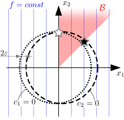
Expected Minimizers
When considering the instance as (CP) then we expect that would be the solution. To see this, notice that is only satisfied at . When , (KKT) becomes ill-conditioned for . Once , the minimizer is suddenly .
When considering the instance as (QPP) then a point close to should be the solution unless becomes large relative in comparison to . To see this, note that minimizes among all points in that yield small relative to .
Scope
Computational Results
We observe that all iterates of all methods remain in . Hence, Theorem 3.2 asserts that MALM and ALM converge because are twice continuously differentiable on and is affine.
We solve the instance with MALM and PM, for various values of , including 0. We implement PM by solving (QPP) directly in IPOPT with objective . Recall that MALM=ALM for and that PM is not applicable (n.a.) when , since is undefined.
Confirmation of Expected Minimizers
We first analyze the limit points (which are identical for both tested methods throughout all tests) for each , by measuring the quantities
Table 1 shows the quantities for respective . Dividing the table into a lower left and an upper right triangle, we see that indeed solutions in the lower triangle are close to and those on the diagonal and in the upper right are close to . This confirms that solutions of (CP) and (QPP) can be very distinct and the latter depend on the value of .
Computational Performance
Table 2 shows the sum of the number of all inner iterations of PM and MALM for respective . We see a trend for each of the two methods: PM converges in a few iterations when is moderate. However, when both decrease, the iteration count blows up. The trend for MALM is different. MALM converges reliably for all in the upper right triangle, including those where are very small.
The last row of Table 2 shows ALM. ALM converges quickly to when . In contrast, when then ALM should converge to but its iteration count blows up for small . In two instances ALM did not converge (n.c.) within iterations. In conclusion, ALM is inefficient when has small inconsistencies.
Rate-of-Convergence Comparison
We compare the rate of local convergence of MALM and ALM to the theoretical prediction from Theorem 3.3. We use and . MALM solves (QPP) with whereas ALM solves (CP). Both minimizers are close to . As shown in Theorem 3.3, local convergence is only linear for our constant choice of . Hence, by Cauchy criterion, converges at the same rate as , where is the exact dual solution. Because is unknown, Figure 3 plots for both methods over the outer iteration index of Algorithm 1. Thereby, we find the rate of convergence for and thus for . We observe convergence at linear rates. We see that both methods converge in very few outer iterations to the order of machine precision. At both methods have roughly attained their limit convergence rates.
2 Integral Penalty-Discretization for Optimal Control
Setting
Initial Guess and Solvers
We solve the instance (2) with MALM and PM for various values of from . Recall that is the mesh size and .
For this example, using the bounded domain , Theorem 3.2 asserts a priori that MALM converges because are twice continuously differentiable on and is affine.
Expected Minimizers
We expect that the optimality gap and feasibility residual
both converge for increasing mesh sizes when choosing ; cf. discussion in Section 2. For too large, should not converge and for too small should not converge. To see this, notice that ; thus, minimization of only strikes a balance between minimizing both terms when is chosen in the right order of magnitude
Scope
We expect that again PM will be faster than MALM when is moderate and vice versa when is very small. We shall also try ALM (i.e., Algorithm 1 with ) but just for completeness, because this will not converge to the optimal control solution.
Computational Results
Confirmation of Expected Minimizers
Table 3 shows the quantities for respective . Dividing the table into a lower left and an upper right triangle, we find our expected minimizers confirmed: solutions in the lower left of the table achieve small but large , whereas solutions in the upper right of the table are not sufficiently feasible with respect to the path-constraints. For a given mesh size , the most accurate control solutions are found on the diagonal cells of the table.
Computational Performance
Table 4 shows the sum of the number of all inner iterations of MALM and PM for respective . We see the same trend as for the circle problem: PM converges faster than MALM when is moderate and vice versa when is small. We underline that MALM converges reliably for all in the upper right triangle, including those where are very small. Needless to say, accurate numerical optimal control solutions require very small; thus MALM seems very attractive for solving these classes of problems.
The last row shows that ALM does not converge (n.c.) within iterations for any mesh size.
5 Conclusions
We presented a modified augmented Lagrangian method (MALM), generalized to non-convex optimization problems with additional inequality constraints. We proved global convergence for our generalized method when the inequalities are affine. A local rate-of-convergence result shows that MALM inherits all the local convergence results of ALM while the regularization in also yields a slight benefit to its rate of local convergence in the iteration limit.
Our numerical experiments demonstrate that MALM outperforms PM when minimizing quadratic penalty programs (QPP) in those situations where is very small, in a similar manner as ALM outperforms PM when solving equality constrained programs (CP). The experiments further show that ALM cannot solve (QPP), but solves (CP) instead. Hence, MALM is the best candidate for solving (QPP) when is very small.
In the experiments we have assumed that the sub-problems (8) are solved to high accuracy. Future work could extend the approach to inexact iterations and sub-iterations to mild tolerances. This could reduce computations at sub-iterations where the dual is far from converged. Another open subject is the extension of global convergence analysis to the cases when is convex nonlinear or non-convex nonlinear.
Chapter 15 Discretization: Integral Penalty Barrier Method
1 Introduction
This chapter presents and analyses a mathematical algorithm for the direct transcription of optimal control problems. In analogy to QPM, we use finite elements and nonlinear programming solvers to solve the optimal control problem as an NLP. However, in contrast to QPM, the method of this chapter uses not only quadratic penalty terms but also logarithmic barrier terms. This yields a better alignment between the merit-functional of the direct transcription and the merit-function of the interior-point algorithm. As motivated in Section 2, this may decrease the number of iterations for the NLP solver to converge. Still, the new way of discretization requires a separate proof of convergence, which is the emphasize of this chapter. The notation of this chapter is independent and uncorrelated to the rest of the thesis. For instance, the functions have different purposes. As another example, the symbol denotes the solution space in this chapter, too, but it uses a different definition from the one in Part 1. Also, there are assumptions (A.1)–(A.5), but these are different from the assumptions that will be used in Part 5 of this thesis.
1 An Important Class of Dynamic Optimization Problems
Many optimal control, estimation, system identification and design problems can be written as a dynamic optimization problem in the Lagrange form
| (DOPa) | ||||
| (DOPb) | ||||
| (DOPc) | ||||
| (DOPd) |
where the open bounded interval , is an appropriately-defined Hilbert space for solution candidates such that is continuous, and “f.a.e.” means “for almost every” in the Lebesgue sense. Detailed definitions and assumptions are given in Section 4. An optimal solution will be denoted with . We note that the form (DOP) is quite general and adopted here to minimize notation.
Ordinary differential equations (ODEs) and path constraints are included via the differential-algebraic equations (DAE) in (DOPc) and the inequalities (DOPd). The point constraints (DOPb) enforce boundary constraints, such as initial or final values on the state , or include values obtained by measurements at given time instances.
With techniques presented in [102, Sect. 3.1],[25, Sect. 2–3],[16, Chap. 4], problems in the popular Bolza or Mayer forms with general inequalities and free initial- or end-time can be converted into the form (DOP). In turn, many problems from control, estimation and system identification can be stated in Bolza or Mayer form [16].
Problem (DOP) is infinite-dimensional, because the optimization is over function spaces subject to an uncountable set of constraints. It is very hard or impossible to compute an analytic solution, in general. Hence, one often has to resort to numerical methods to solve (DOP). When doing so, it is important to eliminate whether features of the numerical solution have arisen from physical principles or numerical failure. The need for a numerical method, which has a rigorous proof that the numerical solution convergences to the exact solution, is therefore essential in practice.
One of the more established choices for the numerical solution of (DOP) is to discretize via direct collocation and finite elements [38, 16, 104, 102, 80]. Recall that explicit Runge-Kutta methods are unsuitable for stiff problems and that many popular implicit methods for solving differential equations, e.g. variants of Gauss schemes, can be interpreted as collocation methods. Collocation methods include certain classes of implicit Runge-Kutta, pseudospectral, as well as Adams and backward differentiation formula methods [80, 16, 104, 4]. However, as is known [16, Sect. 2.5 & 4.14],[33, 77], collocation methods can fail to converge if care is not taken. In [97] we present an example where three commonly used collocation-based direct transcription methods diverge, and below in Section 1 we give a parametric problem for which Legendre-Gauss-Radau collocation [16] of any degree rings.
Notice that (DOP) includes problems with mixed differential and inequality path constraints, for which indirect methods [38, 16] have only a limited range of applicability. Even when applicable, indirect methods require sophisticated user knowledge to set up suitable co-state and switching-structure estimates [20]. A detailed discussion of available methods in the literature is given in Section 7.
There is a scarcity of rigorous proofs that show that high-order collocation schemes for dynamic optimization methods converge to a feasible or optimal solution as the discretization is refined. The assumptions in the literature are often highly technical, difficult to enforce or not very general.
2 Contributions
The penalty-barrier method aims to overcome the limitations of the numerical methods mentioned above by presenting a novel direct transcription method for solving (DOP). Our method combines the following ingredients: quadratic integral penalties for the equality (path) constraints; logarithmic integral barriers for the inequality path constraints; and direct numerical solution via finite elements. It is this combination, together with a rigorous proof of convergence, that amounts to a novel direct transcription method. We also provide order-of-convergence results.
As detailed in Section 4, we only require existence of a solution to (DOP) and mild assumptions on the boundedness and Lipschitz continuity of . In contrast to existing convergence results:
- •
The solution does not need to be unique.
- •
can be non-differentiable everywhere.
- •
We do not require the satisfaction of a constraint qualification for the discretized finite-dimensional optimization problem, such as the Linear Independence Constraint Qualification (LICQ), Mangasarian-Fromovitz Constraint Qualification (MFCQ) or Second-Order Sufficient Conditions (SOSC).
- •
Uniqueness or global smoothness of states or co-states/ adjoints do not need to hold.
- •
Local uniqueness assumptions, as in [94], are removed.
The idea behind our new, Penalty-Barrier-Finite Element method (PBF), is to minimize the following unconstrained penalty-barrier function
| (1) |
where
| (2) |
is the objective,
| (3) | ||||
is the integral quadratic penalty for the equality path- and point constraints, and
| (4) |
is an integral logarithmic barrier for the inequality path constraints. We provide an analysis that shows that one can construct trajectories that converge in the following tolerance-accurate sense: the optimality gap
| (5) |
and feasibility residual
| (6) |
converge to zero as the discretization mesh becomes finer and the parameters converge to zero. Order-of-convergence results will specify the rate at which and approach zero.
The above functions (2)–(4) look similar to those encountered in well-known finite-dimensional penalty-barrier methods. However, in order to deal with the infinite-dimensional nature of the problem, note the use of integrals in the penalty and barrier terms. If the problem had been finite-dimensional in and if had been the squared -norm of finitely many equality constraints, then it would be given that the minimizer of converges to the solution under mild assumptions as converge to zero [50]. The infinite-dimensional case considered here, however, is more involved and requires a careful analysis relating to parameters of the discretization. This is because once we discretize on a mesh and seek to compute an approximate solution on the mesh, the degrees of freedom for depend on the size of the finite element space. If we were to draw an analogy with the finite dimensional case, then the equivalent number of equality constraints depends on the number of quadrature points for numerically evaluating the integral in . If is too large then will not converge to satisfying the equivalent set of equality constraints. If is too small with respect to the mesh size, then there are not enough degrees of freedom, resulting in a potentially feasible but suboptimal solution [63, p. 1078]. The effects of are more intricate, since they relate to a local Lipschitz property of that is relevant for the stability of the finite element discretization. A balance must thus be taken between the size of the finite element space, the quadrature rule and the parameters . This requires a non-trivial analysis, which is the core contribution of this chapter.
3 Motivation from Collocation Methods
We motivate our method from the perspective of collocation methods.
A desirable method for solving optimal control problems is Legendre-Gauss-Radau collocation because it is easy to implement (and high-order consistent): the method constructs piecewise polynomials (of high degree) using a nodal basis and solves the path constraints at a finite number of points. The nodal basis values are determined by solving a large sparse nonlinear program.
However, for solutions with singular arcs, which occur in a large number of applications, the numerical solutions can “ring” [16, Sect. 4.14.1]. In particular, the solution polynomial and the residuals of the path constraints will oscillate between the collocation points — that is, the path residuals will not converge to zero everywhere. A remedy is regularization: a small convex quadratic term is added to the objective to penalize numerical noise. Unfortunately, in most cases this remedy does not work because either the penalty is too small to remove all noise or so large that it alters the problem’s solution.
The idea with the penalty method is to make ringing impossible by adding collocation points inbetween the original collocation points, where otherwise the states, controls and residuals could ring. The theoretical vehicle for this approach are integrals and penalties. Integrals, once discretized by means of numerical quadrature, can be expressed with a set of weights and abscissae, alias collocation points. Penalties, in replacement for exact constraints, will prevent any issues related to the ratio between the number of degrees of freedom and the number of constraints, such as over-determination. The resulting scheme remains easy to implement while effectively forcing global convergence of the path constraints — as we rigorously prove in the remainder of this chapter. In particular, we prove that the feasibility residual converges to zero.
We stress that the integral penalty and log-barrier provide a useful natural scaling for the NLP. This is certainly desirable from a computational perspective, because experience shows that numerical treatment of an NLP depends significantly on scaling [16, Chap. 1.16.5, 4.8]. The large-scale methods in [51, 31] use a merit function that treats equality constraints with a quadratic penalty and inequality constraints with a log-barrier term. Typically, as the NLP becomes larger, caused by a finer discretization, the NLP becomes more challenging to solve, in the sense that the number of iterations to converge increases. In contrast, for the penalty-barrier method the NLP merit function matches the infinite-dimensional merit function in the limit, which mitigates numerical issues that might otherwise arise.
4 Notation
Let and the points , . denotes the closure of . The functions , , . The function and . Given an interval , let . We use Big- notation to analyze a function’s behaviour close to zero, i.e. function if and only if and such that when . The vector with appropriate size.
For notational convenience, we define the function
where . The solution space of is the Hilbert space
with scalar product
| (7) |
and induced norm , where denotes the component of a function . The Sobolev space and Lebesgue space with their respective scalar products are defined as in [1, Thm 3.6]. The weak derivative of is denoted by .
Recall the embedding , where denotes the space of continuous functions over [1, Thm 5.4, part II, eqn 10]. Hence, by requiring that it follows that is continuous. In contrast, though and are in , they may be discontinuous.
5 Assumptions
In order to prove convergence, we make the following assumptions on (DOP):
- (A.1)
(DOP) has at least one global minimizer .
- (A.2)
and are bounded for all arguments within , . is bounded below for all arguments within .
- (A.3)
are globally Lipschitz continuous in all arguments except .
- (A.4)
The two solutions related to , defined in Section 2, are bounded in terms of and . Also, is bounded.
- (A.5)
The related solution can be approximated to an order of at least 1/2 using piecewise polynomials; formalized in (11) below.
Similar assumptions are implicit or explicit in most of the literature. A discussion of these assumptions is appropriate:
- (A.1)
is just to avoid infeasible problems.
- (A.2)
The assumption on can be enforced by construction via lower and upper limits w.l.o.g. because they are (approximately) zero at the (numerical) solution. Boundedness below for is arguably mild when/since are bounded: For minimum-time problems and positive semi-definite objectives this holds naturally. In many contexts, a lower bound can be given. The assumptions on have been made just to simplify the proof of a Lipschitz property and because they mean no practical restriction anyways. The boundedness assumption on is made to avoid unbounded problems.
- (A.3)
can be enforced. Functions that are not Lipschitz continuous, e.g. the square-root or Heaviside function, can be made so by replacing them with smoothed functions, e.g. via a suitable mollifier. Smoothing is a common practice to ensure the derivatives used in a nonlinear optimization algorithm (e.g. IPOPT [120]) are globally well-defined. The assumption has been made to prove a Lipschitz property of a penalty-barrier functional. Actually this property is only needed in a local neighborhood of the numerical optimal control solution, but for ease of notation we opted for global assumptions.
- (A.4)
can be ensured as shown in Remark 7 in Section 2. This assumption effectively rules out the possibility of solutions with finite escape time. The assumption has been incorporated because restriction of a solution into a box means little practical restriction but significantly shortens convergence proofs due to boundedness.
- (A.5)
is rather mild, as discussed in Section 4 and illustrated in Appendix 21.B. All finite-element methods based on piecewise polynomials make similar assumptions, implicitly or explicitly. The assumption is only used for the rate-of-convergence analysis. The assumption is unavoidable, since otherwise a solution could exist that cannot be approximated to a certain order.
The assumptions are not necessary but sufficient. Suppose that we have found a numerical solution. It is not of relevance to the numerical method whether the assumptions hold outside of an open neighborhood of this solution. However, the proofs below would become considerably more lengthy with local assumptions. We outline in Section 8 how our global analysis can be used to show local convergence under local assumptions. Hence, for the same reasons as in some of the literature, we opted for global assumptions. Our analysis is not restrictive in the sense that it imposes global requirements. No further assumptions are made for the proof.
6 Outline
Section 2 introduces a reformulation of (DOP) as an unconstrained problem. Section 3 presents the Finite Element Method in order to formulate a finite-dimensional unconstrained optimization problem. The main result of this chapter is Theorem 6, which shows that solutions of the finite-dimensional optimization problem converge to solutions of (DOP) with a guarantee on the order of convergence.
2 Reformulation as an Unconstrained Problem
The reformulation of (DOP) into an unconstrained problem is achieved in two steps. First, we introduce penalties for the equality constraints. We then add logarithmic barriers for the inequality constraints. The resulting penalty-barrier functional will be treated numerically in Section 3.
Before proceeding, we note that boundedness and Lipschitz-continuity of and in (2)–(3) follow from (A.2)–(A.3).
Lemma 2.1 (Boundedness and Lipschitz-continuity of and ).
is bounded below. is bounded. are Lipschitz continuous in with respect to . Furthermore, are Lipschitz continuous in with respect to the norm .
The proof is given in Appendix 21.C.
We bound the Lipschitz constants (i.e., with respect to both and ) with for and with for .
1 Penalty Form
We introduce the penalty problem
| (PP) |
where and a small penalty parameter . Note that is Lipschitz continuous with constant
| (8) |
with the Lipschitz-constants of and is the upper bound on the 1-norm of , as asserted by (A.2). We show that -optimal solutions of (PP) solve (DOP) in a tolerance-accurate way.
Proposition 2.2 (Penalty Solution).
Proof.
This result implies that for an -optimal solution to (PP) the optimality gap to (DOP) is less than and that the feasibility residual can be made arbitrarily small by choosing the parameter to be sufficiently small.
2 Penalty-Barrier Form
We reformulate (PP) once more in order to remove the inequality constraints. We do so using logarithmic barriers. Consider the penalty-barrier problem
| (PBP) |
where the barrier parameter and is defined in (4).
We have introduced in order to keep feasible with respect to (DOPd). Recall that contains functions that have poles. So the following result is to ensure that actually fulfills its purpose.
Lemma 2.4 (Strict Interiorness).
Proof.
At the minimizer , the functional can be expressed in a single component as
where is Lipschitz-continuous with a constant (cf. right argument in the max-expression (8) and compare to (4) in the proof of Lemma 2.1). From the Euler-Lagrange equation it follows for that
The value of gets closer to zero when the first term grows. However, that term is bounded by the Lipschitz constant. Hence, in the worst case
∎
We will need the following operators:
Definition 2.5 (Interior Push).
Given , define and as a modified whose components have been pushed by an amount into the interior if they are close to zero:
for all and .
Note that and that from Lemma 2.4.
Using the interior push, we show below that is -optimal for (PP). Our result uses a small arbitrary fixed number .
Proposition 2.6 (Penalty-Barrier Solution).
If (A.4) holds, then
Proof.
Remark 7.
Lemma 2 in the proof of Prop. 2.6 needs (A.4), i.e.
Note that the assumption can be enforced. For example, the path constraints
lead to for Constraints like these arise when variables have simple upper and lower bounds before being transformed into (DOP).
Similarly, boundedness of can be enforced. To this end, introduce box constraints for each component of , before transcribing into the form (DOP).
3 Finite Element Method
Our method constructs an approximate finite element solution by solving the unconstrained problem (PBP) computationally in a finite element space , using an NLP solver.
We introduce a suitable finite element space and show a stability result in this space. Eventually, we prove convergence of the finite element solution to solutions of (PBP) and (DOP).
1 Definition of the Finite Element Space
Let the mesh parameter . The set is called a mesh and consists of open intervals that satisfy the usual conditions [35, Chap. 2]:
- 1.
Disjunction: , for all distinct .
- 2.
Coverage: .
- 3.
Resolution: .
- 4.
Quasi-uniformity: . The constant must not depend on and .
We write for the space of functions that are polynomials of degree on interval . Our finite element space is then given as
is a Hilbert space with scalar product .
Note that if , then is continuous but and can be discontinuous. Figure 1 illustrates two functions with and for their nodal basis, to identify them with a finite-dimensional vector.
2 Discrete Penalty-Barrier Problem
We state the discrete penalty-barrier problem as
| (PBPh) |
with the space .
Note that Lemma 2.4 is valid only for solutions to (PBP), whereas below we will consider sub-optimal solutions to (PBPh). Hence, we cannot guarantee that these sub-optimal solutions will satisfy . The looser constraint in the definition above will be used in the proof of Theorem 5.
In a practical implementation, we neglect these additional constraints. This is reasonable when solving the NLP with interior-point methods, since they keep the numerical solution strictly interior with a distance to zero in the order of .
3 Stability
The following result shows that two particular Lebesgue norms are equivalent in the above finite element space.
Lemma 1 (Norm equivalence).
If , then
Below, with the help of Lemma 1, we obtain a bound on the growth of in a neighborhood of a solution to (PBP) for elements in .
Proposition 2 (Lipschitz continuity).
Let
Consider the spherical neighbourhood
The following holds :
Proof 3.2.
From Lemma 2.4 and Lemma 1 follows:
Hence,
| (10) |
From Lipschitz-continuity of we find
We know a lower bound for the arguments in the logarithms from (10). Thus, the essential supremum term can be bounded with a Lipschitz result for the logarithm:
where the latter inequality is obtained using Lemma 1.
4 Interpolation Error
In order to show high-order convergence results, it is imperative that the solution function can be represented with high accuracy in a finite element space. In the following we introduce a suitable assumption for this purpose.
Motivated by the Bramble-Hilbert Lemma [22], we make the assumption (A.5) that for a fixed chosen degree there exists an such that
| (11) |
Notice that the best approximation is well-defined since is a Hilbert space with induced norm . In Appendix 21.B we give two examples to demonstrate the mildness of assumption (11).
To clarify on the mildness of (11), consider the triangular inequality
| (12) |
where is the global minimizer. Clearly, the second term converges under the approximability assumption of finite elements, hence could not be milder. The first term holds under several sufficient assumptions; for instance if is unique because then convergence of feasibility residual and optimality gap will determine –at a convergence rate depending on the problem instance– that unique solution. Due to round-off errors in computations on digital computers, for numerical methods the notion of well-posedness is imperative, hence must always be assumed, relating to how fast the first term converges as optimality gap and feasibility residual converge.
For the remainder, we define , with respect to . We choose and with suitably small such that .
Following the assumption (11), the result below shows that the best approximation in the finite element space satisfies an approximation property.
Lemma 3 (Finite Element Approximation Property).
If (11) holds and is chosen sufficiently small, then
| (13) |
Proof 3.3.
For sufficiently small it follows from , that . Hence,
for some constant . The result follows by noting that
5 Optimality
Theorem 4 (Optimality of Unconstrained FEM Minimizer).
6 Convergence
We obtain a bound for the optimality gap and feasibility residual of .
Theorem 5 (Convergence to (DOP)).
Proof 3.5.
From Theorem 4 we know . This is equivalent to
Since , it follows that and thus . From Lemma 2.4 we know . Thus, we can apply Lemma 2 to bound with . Hence, . Since, according to Proposition 2.6, is -optimal for (PP), where it follows that
In other words, is -optimal for (PP). The result now follows from Proposition 2.2.
Below, we translate the above theorem into an order-of-convergence result.
Theorem 6 (Order of Convergence to (DOP)).
Consider with . Then and .
Proof 3.6.
Recall that , where . If and it follows that .
7 Numerical Quadrature
When computing , usually the integrals in and cannot be evaluated exactly. In this case, one uses numerical quadrature and replaces with . Since is a space of piecewise polynomials, can be integrated analytically. However, the analytic integral expressions become very complicated. This is why, for a practical method, one may also wish to use quadrature for .
If and have been replaced with quadrature approximations , then it is sufficient that these approximations satisfy
| (14) |
with bounded constant and quadrature order , to ensure that the convergence theory holds. We discuss this further below. The constrraint (14) poses a consistency and stability condition.
Consistency
Stability
Beyond consistency, (14) poses a non-trivial stability condition. This is because the error bound must hold . We show this with an example.
Consider , , , and . The constraint forces . Clearly, and are bounded globally. Consider the uniform mesh for , choose for the finite element degree, and Gauss-Legendre quadrature of order , i.e. the mid-point rule quadrature scheme [59] of point per interval. Then, the finite element function , defined as for on each interval, yields the quadrature error
violating (14). In contrast, using Gauss-Legendre quadrature of order (i.e. using quadrature points per interval) yields satisfaction of (14) with .
We see that in order to satisfy (14), a suitable quadrature rule must take into account the polynomial degree of the finite element space and the nature of the nonlinearity of . We clarify this using the notation for function compositions: If
for some , i.e. the integrands of and are polynomials in , then is a sufficient order for exact quadrature. For a practical method, we propose to use Gaussian quadrature of order , i.e. using abscissae per interval .
8 On Local Minimizers
Above, we proved that the global NLP minimizer converges to a (or the, in case it is unique) global minimizer of (DOP). However, practical NLP solvers can often only compute critical points, which have a local minimality certificate at best. For collocation methods, all critical points of (DOP) have convergent critical NLP points if the mesh is sufficiently fine. For PBF the above global convergence result implies a more favorable assertion: For every strict local minimizer of (DOP) there is exactly one convergent strict local NLP minimizer if the mesh is sufficiently fine. Below we explain the reason why this follows from the above global convergence property.
Consider a strict local minimizer of (DOP). By definition of a local minimizer, inactive box constraints could be imposed on (DOP) such that is the unique global minimizer of a modified problem. Upon discretization we would keep the box constraints as . From the above convergence result, since is unique with inactive box constraints, x must converge to , leaving the NLP box constraints inactive, as if they had been omitted as in the original problem.
4 Numerical Experiments
The scope of this paper is the transcription method. Practical aspects in solving the NLP (PBPh) are discussed in [97], where we also show non-zero patterns of the sparse Jacobian and Hessian of the constraints and Lagrangian function; and show that the computational cost roughly compares to solving the NLPs from LGR collocation. Below, we present numerical results for two test problems when using our transcription method and minimizing (PBPh) for the given instance, mesh, and finite element degree.
1 Convex Quadratic Problem with a Singular Arc
Consider a small test problem, which demonstrates convergence of PBF in a case where direct collocation methods ring:
| (15) | ||||||
where is the derivative of , with negative derivative meaning antiderivative. Figure 2 shows the numerical solutions for for Trapezoidal (TR), Hermite-Simpson (HS), LGR collocation and PBF, where the latter two use polynomial degree . For higher degree , LGR would still ring when . TR and HS require box constraints on for boundedness of their NLP minimizers.
2 Second-Order Singular Regulator
This bang-singular control problem from [6] with is given as
| (16) | ||||||
Both LGR and PBF use elements of degree . S has 24507 non-zeros and bandwidth 15 for both discretizations. Forsgren-Gill solves PBF in 40 and LGR in 41 NLP iterations.
Figure 3 presents the control profiles of the two numerical solutions. LGR shows ringing on the time interval of the singular arc. In contrast, PBF converges with the error .
3 Aly-Chan Problem
Both LGR and PBF use elements of degree . S has the same nonzero pattern as before. Forsgren-Gill for PBF/LGR converges in 48/43 iterations. Figure 4 presents the control profiles of the two numerical solutions. PBF converges, with error LGR does not converge for this problem; cf. [76, Fig. 3],[33]. To fix the convergence for this problem, [33] proposes a particular mesh adaptation scheme whereas [76] employs a regularization technique.
4 Regular state-constrained problem
We now consider a test problem for which both types of methods converge with success, so that we can compare conditioning, convergence, and rate of convergence to a known analytical solution:
| s.t. | |||||
The solution is shown in Figure 5.
is constant outside and , between which , yielding .
All methods yield accurate solutions. Figure 6 shows the convergence of the optimality gap and feasibility residual of a respective method. Remarking on the former, we computed and encircled the cross when . Note in the figure that for elements the most accurate solutions in terms of feasibility are found by PBF with . Further, we find that the collocation methods significantly underestimate the optimality value for this experiment.
Now we discuss rates of convergence. Convergence of only first order is expected because higher derivatives of are non-smooth and has edges. Indeed, converges linearly for all methods. PBF5 with stagnates early because it converges to the optimal penalty solution, which for this instance is converged from elements onwards. are then fully determined by . The issue is resolved by choosing smaller. LGR5 and PBF5 with converge similarly, and stagnate at . Due to the high exponent in the objective, small feasibility errors in the collocation methods amount to significant underestimation of the objective.
Finally, we look into computational cost. Solving the collocation methods with IPOPT and the PBF5 discretization with the interior-point method in [51], the optimization converges in iterations for any discretization. Differences in computational cost can arise when one discretization results in much denser or larger problems than others. Here, we compare the sparsity structure of the Jacobian for LGR5 in Figure 7 and PBF5 in Figure 8, each using a mesh size of .
Note that for PBF5, has more rows in the Jacobian than LGR5, thus the Jacobian has hence more non-zeros. However, critical for computations is the primal Schur complement , which is used when solving the KKT system via the reduced form, where D is a diagonal matrix. is a narrow-banded matrix with dense band of the same bandwidth for LGR5 and PBF5.
With regard to computational cost, it follows from Fig. 6 that the ability to choose in PBF can be advantageous. In particular, on coarse meshes, one may opt for small feasibility residual by manually decreasing , whereas with a collocation method one is stuck with the feasibility residual that one obtains for that particular mesh. The figure shows this: For , even on the coarsest mesh the PBF method achieves a solution that has a smaller feasibility residual than other methods on the same mesh. For this problem this becomes possible because the path constraint could be satisfied with zero error by choosing a polynomial of degree 3 (because here PBF uses ).
5 Van der Pol Controller
This problem uses a controller to stabilize the van der Pol differential equations on a finite-time horizon. The problem is stated as
The problem features a bang-bang control with a singular arc on one sub-interval. The discontinuities in the optimal control are to five digits at and .
We solved this problem with LGR collocation on uniform elements of order . We compare this solution to the one obtained with PBF using uniform elements of order , with and .
Figure 9 presents the control profiles of the two numerical solutions. LGR shows ringing on the time interval of the singular arc. In contrast, PBF converges to the analytic solution. The solution satisfies the error bounds , , , and , where . The larger errors in the vicinity of the jumps occur due to the non-adaptive mesh.
6 Reorientation of an Asymmetric Body
This nonlinear problem from [16, Ex. 6.12, eqn. 6.123] in the ODE formulation is considered numerically challenging for its minimum time objective, the control appearing only linearly in the dynamics, the problem having a bang-bang solution and multiple local minima with identical cost. Since the solution is bang-bang, rates of convergence (at least for the optimality gap) can only be linear. We compare convergence of three collocation methods and PBF, where a polynomial degree is used for the -methods.
Using the same initial guess from forward integration of an approximate control solution, LGR and PBF converge on average in 200 iterations. LGR was solved with IPOPT and PBF was solved with a penalty-barrier interior-point method presented in [51]. Both NLP solvers cost one linear system solve per iteration. For , the finite element solution converges to the penalty-barrier minimizer sooner, which however is not very feasible for the DOP at hand. The other collocation methods’ NLPs were also solved using IPOPT, which terminated on local infeasibility for TR and HS. In contrast, LGR and PBF provide numerical solutions that converge at similar rates, which stagnate around for the feasibility residual and for the optimality gap. These methods converge at similar rates. The size of the differential constraint violation and optimality gap for HS, LGR and PBF for different mesh sizes are given in Table 1. For HS, due to box constraints on end-time, which has been expressed as the first state, the optimality gap is negative and equal to the lower box constraint on the first state.
As with any regularization method, good values for can be found on the fly by saving each barrier solution and terminating when differences between subsequent barrier solutions stop decreasing. For computation of the gap, we determined from PBF(3) on 2048 elements, where .
| HS | LGR |
|
|
| |||||||||||
|---|---|---|---|---|---|---|---|---|---|---|---|---|---|---|---|
| 8 |
|
|
|
|
| ||||||||||
| 32 |
|
|
|
|
| ||||||||||
| 128 |
|
|
|
|
| ||||||||||
| 512 |
|
|
|
|
|
7 Obstacle Avoidance Problem
Since we limited our presentation to a convergence analysis for global minimizers, we give this example to demonstrate PBF’s practical capability to also converge to non-global minimizers.
Consider the minimum-time trajectory from to around an obstacle at of radius :
Passing the obstacle above or below results in two locally optimal trajectories. Both are found by PBF, depicted in Figure 10, using the dashed curves as initial guesses (with and computed feasible from via integration and differentiation, respectively) on finite elements of degree 5.
The computed times as in the figure are accurate except to the last digit. The red/black trajectory converges in 52/58 NLP iterations. For comparison, LGR of the same degree and mesh converges in 51/51 iterations. S has 73521 nonzeros and bandwidth 25 for both PBF and LGR.
8 Pendulum in Differential-Algebraic Form
In this example from [17, Chap. 55], a control force decelerates a frictionless pendulum to rest. The objective is to minimize the integral of the square of the control:
with an additional DAE constraint introduced below. The ODE for is a force balance in the pendulum mass. is the control force acting in the direction .
The DAE constraint determines the beam force in the pendulum arm in an implicit way, such that the length remains 1 for all time; [17, Chap. 55] uses
| (17) |
The following alternative constraint achieves the same:
| (17’) |
In the following we study the convergence of TR, HS, LGR () and PBF () on meshes of increasing size. Here, the collocation methods are solved with IPOPT in ICLOCS2, whereas PBF is solved with Forsgren-Gill as before.
TR & HS are likely to converge at a slower rate than PBF & LGR. However, our focus is primarily on determining whether a given method converges, and only secondarily on rates of convergence. To find out where solvers struggle, we consider three variants of the pendulum problem,
- Case A
- Case B
where we add the path constraint .
- Case C
All methods converge for case A. Figure 11 shows that TR converges slowly, while HS, LGR and PBF converge fast. At small magnitudes of , further decrease of LGR and PBF deteriorates, presumably due to limits in solving the NLP accurately under rounding errors.
Case B is shown in Figure 12. The control force decelerates the pendulum more aggressively before the pendulum mass surpasses the lowest point, such that the beam force obeys the imposed upper bound. Figure 13 confirms convergence for all methods. The rate of convergence is slower compared to case A, as expected, because the solution of is locally non-smooth.
For case C, some collocation methods struggle: For HS on all meshes, the restoration phase in IPOPT converged to an infeasible point, indicating infeasibility of (1) for this scheme [120, Sec. 3.3]. For TR, the feasibility residual does not converge, as shown in Figure 14.
Figure 15 shows that this is due to ringing in the numerical solution for the beam force.
Regarding LGR, Figure 14 shows that the feasibility residual converges only for relatively fine meshes. In contrast to the collocation methods, PBF converges as fast as for case A.
Finally, we discuss the computational cost: Using 160 elements, the PBF discretization results in S of bandwidth 30, with 44964 nonzeros for cases A, C and 42951 nonzeros for case B; requiring 66, 51, and 66 NLP iterations for cases A–C. LGR yields the same sparsity pattern for S as PBF, solving on average in IPOPT iterations (with second-order corrections).
5 Conclusions
We presented PBF and proved convergence under mild and easily-enforced assumptions. Key to the convergence proof is the formulation of a suitable unconstrained penalty-barrier problem, which is discretized using finite elements and solved with primal-dual penalty-barrier NLP solvers.
Theorem 6 provides high-order convergence guarantees even if the component has discontinuities, provided that the trajectory can be approximated accurately in the finite element space; see (11) and the discontinuous elements in Figure 1. It is a practical matter to employ an adaptive meshing technique for achieving this in an efficient manner.
The practicality of our novel transcription has been illustrated in numerical examples. The scheme converged for challenging problems, which included solutions with singular arcs and discontinuities. These problems caused issues for three commonly used direct transcription methods based on collocation, namely TR, HS and LGR.
Part 5 Convergence Analysis of Quadrature Penalty Methods
Chapter 16 Introduction
This part presents a proof of convergence for quadrature penalty methods.
We suppose that there exists a local11 1 A global minimizer is a just a special local minimizer minimizer of (1) and we wish to approximate this minimizer numerically. We consider an approximation that is a suitable22 2 In the sense described in Section 1 local minimizer of (4). We prove convergence rates of the measures from Section 3 as . The main result is Theorem 1. We state some notations and a few prerequisites in advance.
1 Notation
Feasible Candidates
We define the space of candidates that satisfy the bound constraints in (4).
Suitable Minimizer
NLPs do often have several different local minimizers. We use an NLP minimizer to construct a numerical optimal control solution to a demanded exact minimizer . However, if our NLP solver picked the wrong then will not converge with respect to but potentially with respect to a different minimizer .
Whenever minimizing locally, one needs a local property to identify the exact local minimizer that is considered. This is why in the following we specify a simple and sufficient characterization of which numerical NLP minimizer we seek. We call such a minimizer a suitable local minimizer. For us, this local property is the objective value.
For each , define an arbitrary fixed pair that satisfies (3), i.e., such that there is a constant such that: (1)Then a suitable numerical local minimizer is any local minimizer of (4) with smaller objective than , i.e.:
| (2) | ||||
Problem (4) certainly has a solution satisfying this bound, because is feasible for (4) and in the extreme case is coincidentally the global minimizer of (4).
2 Prerequisites
We presuppose three properties. We do not pose them as assumptions because two things can be easily agreed upon for each of them: First, the assumptions are inherently necessary in the sense that any numerical method which is based on finite elements must use these assumptions. Second, the assumptions pose an insignificant restriction on the generality of problem instances in the sense that they either hold naturally or can be forced practically with ease.
1 Approximability of Exact Minimizer
We shall require that satisfies the following approximability condition:
There exist finitely above zero, finitely above zero, and finite, such that (3)For short, this can be stated as
Approximability means nothing more than that can be approximated to some order . Sufficient criteria on to satisfy the condition are widely known: For example, [23, Thm. 8.8] bounds the -norm by the -norm. In turn, [47, Prop 1.12] provides orders for the interpolation error in the -norm. Very high orders can be attained for very smooth functions . The following corollary helps for the contrary case when are not very smooth.
Corollary 1.
Let and be -Hölder continuous on each mesh-interval for some . I.e. there exists some finite constant such that for :
| (4) | ||||||
| (5) |
Then (3) is satisfied.
Proof: In Section 10.∎
Remark 2.1.
Some optimal control problems feature solutions with many edges and discontinuities. In this case, by virtue of Corollary 1, convergence with a rate can still be asserted if the mesh is adapted appropriately.
But even when the mesh is not adaptive, the rate is likely . For instance, the convergence of a piecewise linear continuous function to a piecewise constant discontinuous function in the -norm is in .
Insignificance
The prerequisite of approximability is an insignificant restriction because the requirement of Corollary 1 is satisfied for all but the most obscure functions .
Necessity
Like any direct transcription method, we approximate with piecewise polynomials . This approximation is entirely in vain when are not by any means approximatable via piecewise polynomials. Thus, approximability is inherently necessary.
2 Shape of Bound Constraints
To simplify technicalities, we shall require and .
Insignificance
Necessity
Without exact knowledge of their entire shape it is impossible to make assertions on the violation of at any point at which these functions have not been evaluated. Hence, it would be impossible to make assertions on the convergence of from (10).
3 Consistency Order of Quadrature
We shall require that the quadrature rule is of some consistency order according to our definition from (2) in Section 4.
Insignificance
The property can be forced easily in practice by selecting a sufficiently large number of quadrature points.
Necessity
Consistency of quadrature is inherently necessary for convergence whenever integrals are discretized with quadrature. A typical and famous example for this is in the second Strang Lemma [115], where
is necessary to guarantee convergence of a Galerkin method. In Strang’s bound: is a piecewise polynomials space like ; is a functional like ; and is the quadrature approximation of like is the quadrature approximation of . Strang’s requirement on the quadrature’s consistency is virtually identical to ours.
3 Main Result
In Section 3 we introduced the three measures . These measures quantify, in this order, the convergence of optimality for the objective, the convergence of feasibility for the equality constraints, and the convergence of feasibility for the inequality constraints. The following main theorem asserts that these measures indeed converge to zero at a certain order.
Theorem 3.0.
If the below assumptions (A.1), (A.2) and (A.3) from Section 17 hold then the accuracy measures from Section 3 between the exact minimizer and the numerical minimizer of problem (4) satisfy the following bounds:fdsa
The parameter is a Hölder exponent that is introduced in assumption (A.3); reflects the smoothness of the exact minimizer ; and is the quadrature order of .
Proof: in Section 2. ∎
In the experiments we saw that all three measures converge rapidly.
Convergence of can be forced by selecting sufficiently small and then converging . The measure can be decreased by selecting sufficiently large, where is the Chebyshev-Gauss-Lobatto degree in (4), where was defined in (4).
Optimality of the Rates of Convergence
As is known from piecewise polynomial interpolation, a sufficiently smooth function may be at best interpolated with a piecewise polynomial function of degree on a mesh of size with a convergence in . A faster rate cannot be attained. Thus, the rate is called optimal.
Likewise, when an optimal control solution and the problem-defining functions are sufficiently smooth then the convergence measures converge at an optimal rate. In particular, let (i.e., the solution is sufficiently piecewise smooth over the mesh such that the finite elements best-approximation converges in ) and (i.e., the problem-defining functions are at least local Lipschitz continuous). Select a quadrature with such as, e.g., Gauss-Legendre quadrature of sufficient degree. Then .
For , our analysis has focused solely on the most difficult case, i.e., when bound constraint violations may occur due to discontinuities in the exact solution. Due to the discontinuities and hence lack of any smoothness, an order-of-approximation result is unavailable for the rate of convergence of within the scope of our analysis. However, we demonstrate a practical approach below Theorem 1 for the adaptive placement of the number of sampling points in order to obtain high accuracy for satisfaction of inequality constraints.
Chapter 17 All Assumptions
In order to prove Theorem 1, we make use of three assumptions on (1). These three assumptions are labeled (A.1), (A.2), (A.3) and are stated below.
(A.1) Boundedness of Bound Constraints
We assume that there is some finite constant such that
(A.2) Lower Boundedness of Objective
We assume that there is some finite constant such that
To enhance readability, the symbols are templates for arbitrary vectors in .
(A.3) Local Hölder Continuity of
Recall from (1) the problem-defining objective function , the boundary conditions function , and the differential and algrabic equality constraints functions and .
We assume that are Hölder continuous locally around . In particular, we assume that there exist constants , where finitely above zero, finite, and finitely above zero, such that:
| (1a) | ||||
| (1b) | ||||
and
| (2a) | ||||
| (2b) | ||||
and that at each
| (3a) | ||||
| (3b) | ||||
The symbols are templates for vectors in and is a template for vectors in . These symbols are used only in Section 17 and Section 1. Local Hölder continuity is a milder assumption than local Lipschitz continuity.
Chapter 18 Convergence Analysis
The present section provides a convergence analysis, comprising of three theorems. The Main Theorem 1 just summarizes these three theorems.
The separate Section 19 provides illustrated detailed proofs of all theorems and intermediate results. One subsection is dedicated to each proof. Subsection 2 proves Theorem 1.
Since we prove convergence orders, our proofs will use several exponents of and constants . The latter have individual footnotes. The exact formulas of the constants do not matter for the conceptual ideas. We opted to include the formulas anyways, mainly for rigor and for avoidance of excessive big-O notation.
Reminder: The measures measure the convergence of equality feasibility, inequality feasibility, and optimality gap of the numerical optimal control solution. For convergence, they are supposed to converge to zero as decreases.
1 Convergence of
Recall the set of Chebyshev-Gauss-Lobatto points of sampling degree on interval from (4). Further, recall from Section 1 the space of functions that are polynomials of degree on the interval , also depicted in Figure 2 (a).
Theorem 1.0.
Let three scalar functions for some , and let . If satisfy
| (1a) | ||||
| (1b) | ||||
then the following bounds hold :
| (2a) | ||||
| (2b) | ||||
Proof: in Section 3. ∎
The theorem provides a template for each component and on each interval , explained via the following example.
Example for interval-wise applicability of Theorem 1
Consider problem (2): We saw in Figure 2 that of degree suffers from Gibbs’ phenomenon on . To avoid the overshoot, we may choose sampling points for the bound constraints of on the particular interval where the overshoot occurs. Thereby, Theorem 1 asserts that the overshoot will be no more than
In general, the term converges to zero as is increased.
2 Convergence of and
The next theorem proves convergence of subject to the condition that the numerical minimizer achieves a certain optimality gap to the exact minimizer, denoted with . The subsequent theorem shows that this gap indeed converges.
Theorem 1.
Proof: in Section 4. ∎
As the next theorem shows, for the measure converges. For the theorem, recall from (3), the piecewise polynomials quadrature order from Section 3, and the Hölder exponent from (A.3).
Theorem 2.
| If (A.3) holds and is sufficiently small |
then there exists some finite constant such that the following bound holds:
| (4) |
3 Fundamental Lemma
In preparation for the next section, we introduce a fundamental lemma, that is critical for the proof of many intermediate results. We now explain the purpose of the lemma. Afterwards, we state the lemma.
Some of our results make use of assumption (A.3). Usually, the bounds from (A.3) cannot be used directly because they hold only locally. For example, (1a) gives a bound that only holds when the locality condition (1b) is satisfied.
Thus, before showing any further results, we will prove up-front that the bounds from (A.3) can be used directly for from Section 1.
Lemma 1 (Fundamental Lemma).
Proof: in Section 1.∎
Chapter 19 Proofs of all Theorems
Theorem 1 asserts convergence of several measures and a rate-of-convergence result for each of these measures. By itself, this necessitates a complex proof. A complex proof should not incentivize one to opt for proving a weaker result instead or to forego any helpful details.
Given the result and the volume of its proof, we decided to encapsulate as many intermediate results as possible. This shortens each individual proof but leads to a multitude of small lemmas. Figure 1 gives a dependency graph of all proofs and assumptions. As shown in the figure, the majority of the proofs are on an intermediate result that is used for the proof of Theorem 2.
1 Proof of the Fundamental Lemma 1
Structure of the Proof
Recall the parameter from (A.3). The proof depends on the following two norms:
| (1a) | |||
| (1b) | |||
If is sufficiently small then both norms are smaller than . A sufficiently small value for is developed in Section 1. Afterwards, Sections 2 and 3 prove bounds for each of the above norms. Finally, Sections 4, 5, 6 in turn use these bounds to show the propositions (5a), (5b), (5c), respectively.
1 A Sufficiently Small Value for
By requirement, is sufficiently small. Thus, we may consider
| (2) |
for the purpose that
| (3) |
2 Bound of Norm (1a)
3 Bound of Norm (1b)
4 Proof of (5a)
5 Proof of (5b)
Notice that satisfies the boundary conditions
| (6) |
exactly because is an exact solution.
6 Proof of (5c)
2 Proof of Main Theorem 1
From here on, we dedicate one subsection into the proof of one theorem or lemma. This subsection is the proof of Theorem 1. Recall that you can go back and forth via the embedded hyperlinks.
Structure of the Proof
We first introduce a bound for . This helps us bound . Afterwards, we prove convergence of via straightforward application of Theorem 1.
Convergence Order of and
Convergence Order of
3 Proof of Theorem 1
The proof makes use of the following corollary.
Corollary 1.
Let . Then
Proof: in [13, Summae Potestatum]. ∎
Strategy of the Proof
The sampling conditions (1a) guarantee satisfaction of the constraints only at the sampling points , whereas we want to bound the maximum violation of in between any two neighboring sampling points. This is achieved by bounding the curvature of a transformed version of .
Structure of the Proof
In Figure 2 (b), we consider a rescaled version of such that the lower bound (blue curve) is a constant of . We then perform a cosine transformation from Figure 2 (b) into a function in Figure 2 (c). Both transformations are given in Section 1.
1 Transformation into a Finite Cosine Series
We uniquely identify with functions such that and :
| (9a) | ||||
| (9b) | ||||
| (9c) | ||||
The functions are plotted in Figure 2 (b).
Using a change of variable for into via the relation22 2 the negative sign is to be consistent with the literature convention in [125] for Chebyshev-Gauss-Lobatto points from (4). This is so are increasing as increases. , we define the function . Because , we may express as a series of Chebyshev polynomials of the first kind33 3 The Chebyshev polynomial on can be expressed as , thus:
| (10) | ||||
| (11) |
with coefficients .
Figure 2 shows an example of for , , and . Notice that the Chebyshev-Gauss-Lobatto points from (4) become equidistant as the variable changes into . The points are equidistant due to the -transformation of the points from (4). This can be observed in Figure 2 (c), where all crosses and circles are equidistant. Recall that the circles in Figure 2 indicate each sampling point. There are encircled points. We can check that the transformed points from (4) satisfy
| (12) |
As apparent from (12), the points only depend on and not on . Figure 2 (d) illustrates the sampling points (with symbol ) over each sampling point (with symbol ).
Lemma 2.
Assign the vectors , for the quantities in (11). The following relation holds in general:
Proof: in Section 6. ∎
2 Bounding the Curvature
3 Construction of a Worst-Case Estimate
Thus far, we obtained the bound for from using only the encircled black and blue sampling points in Figure 2 (c). These points are invariant to , hence why the bound holds . Now, we use the blue crossed sampling points. They are spaced with distance .
Construct the violet parabola with and , i.e., the parabola that interpolates two neighboring blue crossed sampling points and has curvature , as depicted in the lower left of Figure 2 (c). Parabolas like can be used to bound the value of everywhere in-between the sampling points. This is depicted with the dashed violet graph in Figure 2 (c). The dashed graph consists of successive replicas of .
For , polynomial interpolation yields the parabola of the solid violet graph as
| (13) |
We can check that , , and . Logically, the minimum of is at , thus . Hence, is bounded below by . Back-transformation from into via (9) introduces the factor , completing the proof.
4 Proof of Theorem 1
First Proposition
Second Proposition
5 Proof of Theorem 2
For the scope of this proof, we make use of the following two functionals:
| (15) | ||||
| (16) |
The second functional is a quadrature-approximation of the first. The following lemma asserts an error bound on the quadrature.
Lemma 1.
Let and . If
| (17) |
then
Proof: in Section 7. ∎
Lemma 2.
| If (A.3) holds and is sufficiently small |
then there exists a finite constant such that:
| (18) |
Proof: in Section 8. ∎
We now present the actual proof of Theorem 2.
Structure of the Proof
1 Bound for
2 Bound for
6 Proof of Lemma 2
We may write (11) as
| (21) |
where is the symmetric matrix with entries for , where from (12). Also, define . As known from discrete cosine transform of first kind [116], the matrix is orthogonal. Multiplying from the left onto (21) and inserting an identity matrix yields:
Using orthogonality of G, the following relation is implied for the norms:
| (22) |
Use submultiplicativity, i.e.:
| (23a) | ||||||
| (23b) | ||||||
Using (23b) for the left-hand side of (22) and (23a) for the right-hand side of (22), we obtain:
The proposition follows from and bounding . A variant of Lemma 2 is known as Parseval’s identity. This variant is subject to different scalings, notations, and not for the cosine but for the Fourier transformation.
7 Proof of Lemma 1
8 Proof of Lemma 2
Our proof makes use of the following lemma. The function therein is defined in (2).
Proof: in Section 9. ∎
9 Proof of Lemma 1
We use the following intermediate result.
Corollary 1.
Let and for some . Then:
Proof:
| write out definition | ||||||
| multiply out | ||||||
| bound cross term by abs | ||||||
| apply Cauchy-Schwarz | ||||||
| bound generously | ||||||
Now that we have finished the proof of the intermediate result, we come to the actual proof of Lemma 1. It works by first bounding the integrand and then integrating over the bound.
Bounding the Integrand
Integrating over the Bound
10 Proof of Corollary 1
Structure
We first show pointwise interpolation errors for . We then show (3) by integrating over these pointwise error-bounds.
1 Pointwise Errors
Pick an arbitrary . Wlog., assume . Choose arbitrarily.
On , interpolate piecewise linear:
| (29) |
Since the mean-value theorem does not work when has edges44 4 Example: , then for any ., we use the following trick with the convex hull:
| (30) | ||||||
| (31) |
Hence:
| insert (29) (red) | |||||
| use (30) | |||||
| add zero (blue) | |||||
| drop zero term | |||||
| bound diameter | |||||
| use (4) | |||||
| use |
Likewise, the derivative can be bounded:
| differentiate (29) | |||||
| bound distance | |||||
| use (4) |
Now, choose arbitrarily. On , interpolate piecewise constant:
| (32) |
Hence:
Finally, we can use and likewise for . In conclusion, the following bounds hold :
2 Integral Errors
Chapter 20 Conclusions on QPM
We have seen that QPM and DCM are very similar in their computational structure and expense, but very different in terms of robustness: QPM converges in practically relevant instances where DCM does not converge. The theory presented here explains why QPM converges for a large set of possible circumstances.
In contrast to prevailing opinion, QPM does in fact converge regardless of singular arcs or high-index differential-algebraic constraints. This has been confirmed here with both a proof and with numerical experiments. In contrast, DCM does sometimes not converge for singular arc problems, as is known in theory and as has been confirmed here by our numerical experiments.
When faced with having to choose a method for solving optimal control problems, and if you cannot foresee whether any of these problems may have singular arcs or any of the other features where DCM fails, then QPM is a suitable first resort.
Part 6 Conclusions and Recommendations
Chapter 21 Conclusions
We have presented three numerical methods: For the mathematical problem class of dynamic optimization we presented a direct quadratic penalty transcription method (QPM) and a direct penalty-barrier transcription scheme. These transcription schemes result in NLPs with large quadratic penalty terms. We presented MALM as a tailored solution algorithm for treating these NLPs more efficiently and reliably. Conclusions on each method have been given in the respective chapters.
1 Possible Impacts
In the following we will forecast impacts that the presented research could have on developments in mathematical methods for the numerical solution of optimization problems and of optimal control problems.
Replacement of Collocation Methods
Penalty-based direct transcription methods are structurally very similar to collocation methods; in part because they generalize them. Yet, they can offer significant improvements to the robustness (i.e., reliability of convergence) and the rate of convergence over collocation methods. Both classes of methods are of the same computational cost, judged from identical sparsity patterns in their reduced Newton equations and similar iteration counts in the NLP solvers. The NLPs of QPM and DCM are constructed in a very similar way, as evident from comparision of Section 3 and Section 2. QPM’s overhead, discussed along Figure 2, results from the fact that QPM uses some additional quadrature points in comparison to the number of collocation points that DCM uses.
Paradigm Shift in NLP Solver Templates
Current software for the solution of NLP in form (1) assumes that the equality-constraints describe a subdomain of feasible points in the search space . For example, SNOPT and IPOPT assume that the number of equality constraints do not exceed the dimension of . In concrete terms, when then where is assumed by SNOPT. In the light of QPM and in the light of NLP instances that originate from problems where the search space and constraint space is infinite, those concepts seem unjustified.
We believe that there should be three classes of NLP solver templates:
- 1.
Small dense: These problems may indeed assume that . Solvers can use active sets, null-space projection, or – in case the constraints are linear – orthogonalize the rows of the constraint Jacobian.
- 2.
Large sparse: These problems may still assume that . Due to practicality, solvers must make compromises when attempting to leverage the techniques from small dense problems.
- 3.
From discretization: These problems are finite-dimensional discretizations of infinite-dimensional optimization problems. For discretized problems, constraints and search spaces are to be treated as approximate projections from infinite-dimensional spaces; hence concepts such as exactly feasible points and all the geometric ideas of small dense problems must be abandoned, such as, e.g.,: orthogonalizability of constraint Jacobian rows, second-order corrections, exact Lagrange multipliers, dual boundedness, active sets, reduced Hessians, not to forget “presolve”, and everything relating to non-regularized KKT conditions. Another aspect that is important for problems from discretization is an interface for the supply of quadrature weights to the NLP solver. In particular, we wish to supply barrier weights for the integral log-barrier that is inherited in primal-dual IPM, as this can enable mesh-independent rates of convergence.
For the last class there virtually exists no solid open-source software project. In [93] we had already developed a numerically stable interior-point method that does not consider equations as equality constraints as a description of a geometric subdomain but instead as a measure that shall be bounded by another value that is implicitly given from the problem instance. This is more generic and in alignment with what we need for discretized infinite-dimensional optimization problems.
A last aspect, that will also be critical for the practical utility of NLP solvers for the third category, is a suitable standard interface for continuous-level information. Particularly for direct transcription applications for the optimal control of PDE, it is necessary to define a suitable preconditioner interface. This interface should forsee NLP iterations on various levels of the discretization (nonlinear multi-grid method) and different strategies of preconditioning (null-space preconditioners, constraint-space preconditioners, domain decomposition, etc.). Each different strategy requires a different interweaving between the preconditioner and the NLP solver iteration.
2 Recommendations for Future Research
We suggests the following possible directions.
Mesh Refinement
We have not presented mesh refinement strategies for QPM. This should work in an identical fashion to mesh refinement for DCM. Notably, in QPM we do not only have the mesh that we can adapt but we can also choose of different magnitude on different segments of the mesh. For instance, when solving on and finding larger errors over the sub-domain then it makes sense to choose .
NLP Software for Problems from Discretization
In the present landscape, there is a jungle of proprietary software for LP, QP, convex QP, and NLP. We are not aware of solvers for problems from discretization, according to our standards. Such a method would offer a bias-parameter like and interfaces for matrices S, such that ), W of constraint quadrature weights, and G, such that . This results in different formulas for the central path, the primal-dual equations, the convergence complexity, solution accuracy, numerical stability, and practical performance.
GPU Parallelism
We have not yet implemented optimal control solvers on GPU. Because the computational step (N.2) in our presented NLP solver is massively parallel, there is huge potential for GPU-accelerated versions of QPM. The challenge is with suitable GPU hardware. Since the matrices involved are sparse, the compute intensity is relatively low. This implies that GPU-internal RAM and PCIe bus form a computational bottleneck.
Part 7 Appendices
Appendix 21.A Lebesgue Equivalence for Polynomials
Let and . We show that
Choose arbitrary. Since holds for both , and for all , w.l.o.g. let . Since is arbitrary, w.l.o.g. let for some . Define , , , and Since , it holds . Figure 1 illustrates for .
Use , where is linearly transformed from onto . Since is invariant under changes of because , w.l.o.g. we can assume for that and hence . Since minimizing the -norm, solves
| (1) |
Appendix 21.B Order of Approximation for Non-smooth and Continuous Non-differentiable Functions
In the following we illustrate that the assumption in (11) is rather mild. To this end, we consider two pathological functions for . In our setting, , and we interpolate a given pathological function with over . We use .
A function with infinitely many discontinuities
The first example is a non-smooth function that has infinitely many discontinuities. Similar functions can arise as optimal control solutions; cf. Fuller’s problem [53].
Consider the limit of the following series:
switches between and whenever halves its distance to . Figure 2 shows for .
A continuous but nowhere differentiable function
Consider the following Weierstrass function, which is continuous but non-differentiable:
for . This function with range satisfies the Hölder property with some for [127]. For we have .
According to this property, a piecewise constant interpolation of satisfies . In conclusion, . Therefore, all satisfy (11).
Appendix 21.C Proof of Lemma 2.1
The boundedness follows from (A.2).
Lipschitz continuity of is not as straightforward. We will make use of the following trace theorem [44]: For an open interval it holds that with a constant independent of . Assume attains its essential supremum on at . Choosing , then Using this together with the above bound and results in
| (3) |
Below, for a generic Lipschitz continuous function with Lipschitz-constant and -bound , we use the relation
| (4) | ||||
where we used in the first line and the triangular inequality in the second line. Using the above bound, we can show Lipschitz continuity of :
where (3) has been used to bound .
If then we see the result shows Lipschitz continuity of with respect to . Using
according to [1, Thm. 2.8, eqn. 8], and the definition of , we arrive at
which shows Lipschitz continuity of with respect to .
Lipschitz continuity of follows from Lipschitz continuity of :
Appendix 21.D Properties of the -Barrier Function
Let be a fixed small arbitrary number.
Lemma 1 (Order of the Term).
It holds:
Proof 21.D.1.
We use from (8), where and . We get
In the third line above, we used the fact that for , follows The result follows from , as we show using L’Hôpital’s rule:
Lemma 2 (Bound for ).
If with , then
Proof 21.D.2.
Since the definitions are similar, we only show the proof for :
| (5) |
In the third line, we distinguished two cases, namely attains its essential supremum at a where either (case 1) or where (case 2). In the first case, we can use Lemma 2.4 & 1. In the second case, we simply bound the logarithm using to arrive at the term in the brackets. The final line follows from the fact that .
List of Symbols
| Optimal Control Functions | |
| time | |
| function of ; states | |
| function of ; controls | |
| time-derivative of | |
| the vectorial component of | |
| the vectorial component of | |
| number of states | |
| number of controls | |
| Optimal Control Problem | |
| final time | |
| objective | |
| function of and ; boundary conditions | |
| function of , , and ; differential equations right-hand side | |
| function of , , and ; algebraic equations | |
| function of , , , and ; short-hand for differential and algebraic equations | |
| function of ; left bounds on | |
| function of ; right bounds on | |
| Mesh | |
| mesh point index | |
| number of mesh intervals | |
| mesh points, from to | |
| mesh interval | |
| mesh size | |
| Explicit Euler approximations to | |
| Local Minimizers | |
| an exact local minimizer of the optimal control problem | |
| a numerical local minimizer of the optimal control problem | |
| an approximation of on the mesh | |
| local minimizer of an optimization problem | |
| Solution Measures | |
| optimality gap | |
| constraint violation measure; functional of | |
| equality feasibility residual | |
| inequality feasibility residual | |
| Piecewise Polynomials | |
| piecewise polynomials degree | |
| continuous piecewise polynomials function of degree | |
| discontinuous piecewise polynomials function of degree | |
| space of all of degree and of degree | |
| Collocation | |
| a set of collocation points in | |
| a set of collocation points on each mesh interval | |
| set of all Chebyshev-Gauss-Lobatto points of degree | |
| set of all Chebyshev-Gauss-Lobatto points of degree | |
| Reference Conventions | |
| natural number | |
| real numbers | |
| real vectors | |
| reference interval | |
| a number on | |
| the -transformation of into | |
| vectorial functions in space | |
| scalar functions of | |
| scalar functions of | |
| scalar function in space | |
| derivative with respect to | |
| foot-indices for left and right bounds on quantities | |
| F | Fourier-type matrices |
| G | unitary matrices |
| D | diagonal matrices |
| NLP | |
| x | local minimizer |
| dimension of minimizer | |
| number of equality constraints | |
| f | objective function, mapping into |
| c | equality constraints function, mapping into |
| 1 | vector of ones |
| 0 | vector of zeros |
| I | identity matrix |
| A | matrix of affine inequality constraints |
| left/right inequality constraints vectors | |
| y | Lagrange multipliers vector for equality constraints |
| Lagrange multipliers vector for left/right inequality constraints | |
| dimension of | |
| Constrained Optimization Algorithm | |
| H | Hessian of the Lagrangian |
| J | Jacobian of the equality constraints |
| S | reduced Newton Matrix |
| Newton step for x | |
| Newton step for y | |
| Newton step for | |
| Newton step for | |
| w | stacked vector of |
| merit function, mapping w into | |
| penalty parameter of the interior-point method | |
| barrier parameter of the interior-point method | |
| maximum step size for the line-search | |
| line-search step size | |
| stacked vector of | |
| Quadrature | |
| set of quadrature points with their respective quadrature weights per mesh interval | |
| quadrature degree | |
| short-hand writing for the quadrature formula | |
| Orders | |
| piecewise polynomials quadrature order | |
| mesh interpolation order | |
| Hölder exponent | |
| Factors | |
| piecewise polynomials quadrature factor | |
| interpolation factor | |
| Hölder factor | |
| Bounds | |
| in (A.1); maximum diameter between and | |
| in (A.2); lower bound on | |
| in (A.3); neighborhood margin of Hölder continuity | |
| in (A.3); template for vectors in | |
| in (A.3); template for vector in | |
| Convergence Analysis | |
| equals | |
| in Fundamental Lemma 1; equals | |
| in Fundamental Lemma 1; equals | |
| in Fundamental Lemma 1; equals | |
| equals | |
| equals | |
| Spaces | |
| all functions that are polynomials of degree over | |
| Hölder space | |
| Lebesgue space | |
| Sobolev space | |
| Candidate space | |
| Space of feasible candidates | |
| Space of functions that are polynomials on an interval | |
| Piecewise polynomials space | |
| Space of feasible candidates to (4) | |
| Norms | |
| Euclidean norm | |
| maximum norm | |
| Lebesgue norm | |
| Sobolev norm | |
| Sobolev norm | |
| Operators | |
| transpose of A | |
| diagonal matrix with entries of x |
References
- Adams [1975] R. A. Adams. Sobolev spaces. Academic Press [A subsidiary of Harcourt Brace Jovanovich, Publishers], New York-London, 1975. Pure and Applied Mathematics, Vol. 65.
- Ahmadi [2016] A. A. Ahmadi. Sum of squares (SOS) techniques : An introduction, 2016. URL http://www.princeton.edu/˜amirali/Public/Teaching/ORF523/S16/ORF523_S16_Lec15.pdf.
- Aly and Chan [1973] G. M. Aly and W. C. Chan. Application of a modified quasi-linearization technique to totally singular optimal problems. International Journal of Control, 17:809–815, 1973.
- Arévelo et al. [2002] C. Arévelo, C. Führer, and M. Selva. A collocation formulation of multistep methods for variable step-size extensions. Applied Numerical Mathematics, 42(1–3):5–16, August 2002.
- Armand et al. [2014] P. Armand, J. Benoist, R. Omheni, and V. Pateloup. Study of a primal-dual algorithm for equality constrained minimization. Comput. Optim. Appl., 59(3):405–433, 2014. ISSN 0926-6003. 10.1007/s10589-014-9679-3. URL https://doi.org/10.1007/s10589-014-9679-3.
- Aronna et al. [2013] M. S. Aronna, J. F. Bonnans, and P. Martinon. A shooting algorithm for optimal control problems with singular arcs. J. Optim. Theory Appl., 158(2):419–459, 2013. ISSN 0022-3239. 10.1007/s10957-012-0254-8. URL https://doi.org/10.1007/s10957-012-0254-8.
- Ascher [1978] U. Ascher. Discrete least squares approximations for ordinary differential equations. SIAM J. Numer. Anal., 15(3), June 1978.
- Augustin and Maurer [2001] D. Augustin and H. Maurer. Sensitivity analysis and real-time control of a container crane under state constraints. In Online Optimization of Large Scale Systems, pages 69–82. Springer, 2001.
- Babuška [1973] I. Babuška. The finite element method with penalty. Math. Comp., 27:221–228, 1973. ISSN 0025-5718. 10.2307/2005611. URL https://doi.org/10.2307/2005611.
- Balakrishnan [1968] A. V. Balakrishnan. On a new computing technique in optimal control. SIAM J. Control, 6:149–173, 1968. ISSN 0363-0129.
- Battin [1999] R. H. Battin. An introduction to the mathematics and methods of astrodynamics. Aiaa, 1999.
- Bellman [1954] R. Bellman. Dynamic programming and a new formalism in the calculus of variations. Proc. Nat. Acad. Sci. U.S.A., 40:231–235, 1954. ISSN 0027-8424. 10.1073/pnas.40.4.231. URL https://doi.org/10.1073/pnas.40.4.231.
- Bernoulli [1713] J. Bernoulli. Ars conjectandi. Impensis Thurnisiorum, fratrum, 1713.
- Bertsekas [1982] D. P. Bertsekas. Constrained optimization and Lagrange multiplier methods. Computer Science and Applied Mathematics. Academic Press, Inc. [Harcourt Brace Jovanovich, Publishers], New York-London, 1982. ISBN 0-12-093480-9.
- Betts [1998] J. T. Betts. Survey of numerical methods for trajectory optimization. Journal of guidance, control, and dynamics, 21(2):193–207, 1998.
- Betts [2009] J. T. Betts. Practical Methods for Optimal Control and Estimation Using Nonlinear Programming. Cambridge University Press, New York, NY, USA, 2nd edition, 2009. ISBN 0898716888, 9780898716887.
- Betts [2015] J. T. Betts. A collection of optimal control test problems, 2015. URL http://www.appliedmathematicalanalysis.com/downloads/prbook.pdf.
- Bock and Plitt [1984] H. Bock and K. Plitt. A multiple shooting algorithm for direct solution of optimal control problems*. IFAC Proceedings Volumes, 17(2):1603–1608, 1984. ISSN 1474-6670. https://doi.org/10.1016/S1474-6670(17)61205-9. URL https://www.sciencedirect.com/science/article/pii/S1474667017612059. 9th IFAC World Congress: A Bridge Between Control Science and Technology, Budapest, Hungary, 2-6 July 1984.
- Boffi et al. [2013] D. Boffi, F. Brezzi, and M. Fortin. Mixed finite element methods and applications, volume 44 of Springer Series in Computational Mathematics. Springer, Heidelberg, 2013. ISBN 978-3-642-36518-8; 978-3-642-36519-5. 10.1007/978-3-642-36519-5. URL https://doi.org/10.1007/978-3-642-36519-5.
- Böhme and Frank [2017] T. J. Böhme and B. Frank. Indirect Methods for Optimal Control, pages 215–231. Springer International Publishing, Cham, 2017. ISBN 978-3-319-51317-1. 10.1007/978-3-319-51317-1_7. URL https://doi.org/10.1007/978-3-319-51317-1_7.
- Boltyanskiĭ et al. [1956] V. G. Boltyanskiĭ, R. V. Gamkrelidze, and L. S. Pontryagin. On the theory of optimal processes. Dokl. Akad. Nauk SSSR (N.S.), 110:7–10, 1956. ISSN 0002-3264.
- Bramble and Hilbert [1970] J. H. Bramble and S. R. Hilbert. Estimation of linear functionals on Sobolev spaces with application to Fourier transforms and spline interpolation. SIAM J. Numer. Anal., 7:112–124, 1970. ISSN 0036-1429. 10.1137/0707006. URL https://doi.org/10.1137/0707006.
- Brezis [2010] H. Brezis. Functional Analysis, Sobolev Spaces and Partial Differential Equations. Universitext. Springer New York, 2010. ISBN 9780387709130.
- Bryson [1999] A. E. Bryson. Dynamic optimization. Prentice Hall, 1999.
- Bryson and Ho [1975] A. E. Bryson, Jr. and Y.-C. Ho. Applied Optimal Control: Optimization, Estimation, and Control. Taylor & Francis Group, New York (NY), 1975. ISBN 0891162283.
- Buluç and Gilbert [2012] A. Buluç and J. R. Gilbert. Parallel sparse matrix-matrix multiplication and indexing: implementation and experiments. SIAM J. Sci. Comput., 34(4):C170–c191, 2012. ISSN 1064-8275. 10.1137/110848244. URL https://doi.org/10.1137/110848244.
- Bunch and Kaufman [1977] J. R. Bunch and L. Kaufman. Some stable methods for calculating inertia and solving symmetric linear systems. Math. Comp., 31(137):163–179, 1977. ISSN 0025-5718. 10.2307/2005787. URL https://doi.org/10.2307/2005787.
- Büskens and Wassel [2013] C. Büskens and D. Wassel. The ESA NLP solver WORHP. In Modeling and optimization in space engineering, volume 73 of Springer Optim. Appl., pages 85–110. Springer, New York, 2013. 10.1007/978-1-4614-4469-5_4. URL https://doi.org/10.1007/978-1-4614-4469-5_4.
- Byrd et al. [2006] R. H. Byrd, J. Nocedal, and R. A. Waltz. KNITRO: An integrated package for nonlinear optimization. In Large-scale nonlinear optimization, volume 83 of Nonconvex Optim. Appl., pages 35–59. Springer, New York, 2006. 10.1007/0-387-30065-1_4. URL https://doi.org/10.1007/0-387-30065-1_4.
- Campbell and Kunkel [2016] S. Campbell and P. Kunkel. Solving higher index dae optimal control problems. Numerical Algebra, Control & Optimization, 6(4):447, 2016.
- Cao et al. [2016] Y. Cao, A. Seth, and C. D. Laird. An augmented Lagrangian interior-point approach for large-scale NLP problems on graphics processing units. Computers and Chemical Engineering, 85:76–83, 2016. ISSN 0098-1354. https://doi.org/10.1016/j.compchemeng.2015.10.010. URL http://www.sciencedirect.com/science/article/pii/S0098135415003257.
- Cauchy et al. [1847] A. Cauchy et al. Méthode générale pour la résolution des systemes d’équations simultanées. Comp. Rend. Sci. Paris, 25(1847):536–538, 1847.
- Chen and Biegler [2016] W. Chen and L. T. Biegler. Nested direct transcription optimization for singular optimal control problems. AIChE Journal, 62(10):3611–3627, 2016. 10.1002/aic.15272. URL https://aiche.onlinelibrary.wiley.com/doi/abs/10.1002/aic.15272.
- Chyba et al. [2009] M. Chyba, E. Hairer, and G. Vilmart. The role of symplectic integrators in optimal control. Optimal Control Applications & Methods, 30:367–382, 2009.
- Ciarlet [1978] P. G. Ciarlet. The finite element method for elliptic problems. North-Holland Publishing Co., Amsterdam-New York-Oxford, 1978. ISBN 0-444-85028-7. Studies in Mathematics and its Applications, Vol. 4.
- Conn et al. [1992] A. R. Conn, N. I. M. Gould, and P. L. Toint. Lancelot, volume 17 of Springer Series in Computational Mathematics. Springer-Verlag, Berlin, 1992. ISBN 3-540-55470-x. 10.1007/978-3-662-12211-2. URL https://doi.org/10.1007/978-3-662-12211-2. A Fortran package for large-scale nonlinear optimization (release A).
- Conn et al. [1996] A. R. Conn, N. Gould, A. Sartenaer, and P. L. Toint. Convergence properties of an augmented Lagrangian algorithm for optimization with a combination of general equality and linear constraints. SIAM J. Optim., 6(3):674–703, 1996. ISSN 1052-6234. 10.1137/s1052623493251463. URL https://doi.org/10.1137/S1052623493251463.
- Conway [2012] B. A. Conway. A Survey of Methods Available for the Numerical Optimization of Continuous Dynamic Systems. Journal of Optimization Theory and Applications, 152(2):271–306, Feb 2012. ISSN 1573-2878. 10.1007/s10957-011-9918-z. URL https://doi.org/10.1007/s10957-011-9918-z.
- Courant [1943] R. Courant. Variational methods for the solution of problems of equilibrium and vibrations. Bull. Amer. Math. Soc., 49:1–23, 1943. ISSN 0002-9904. 10.1090/s0002-9904-1943-07818-4. URL https://doi.org/10.1090/S0002-9904-1943-07818-4.
- Cullum [1969] J. Cullum. Discrete approximations to continuous optimal control problems. SIAM J. Control, 7:32–49, 1969. ISSN 0363-0129.
- Cuthrell and Biegler [1989] J. E. Cuthrell and L. T. Biegler. Simultaneous optimization and solution methods for batch reactor control profiles. Computers & Chemical Engineering, 13(1-2):49–62, 1989.
- De Julio [1970] S. De Julio. Numerical solution of dynamical optimization problems. SIAM J. Control, 8:135–147, 1970. ISSN 0363-0129.
- Dieudonné [1976] J. Dieudonné. Treatise on analysis. Vol. II, volume 10 of Pure and Applied Mathematics. Academic Press [Harcourt Brace Jovanovich, Publishers], New York-London, 1976. ISBN 0-12-215502-5. Enlarged and corrected printing, Translated by I. G. Macdonald, With a loose erratum.
- Ding [1996] Z. Ding. A proof of the trace theorem of Sobolev spaces on Lipschitz domains. Proc. Amer. Math. Soc., 124(2):591–600, 1996. ISSN 0002-9939. 10.1090/s0002-9939-96-03132-2. URL https://doi.org/10.1090/S0002-9939-96-03132-2.
- Dontchev et al. [2000a] A. L. Dontchev, W. W. Hager, and K. Malanowski. Error bounds for Euler approximation of a state and control constrained optimal control problem. Numer. Funct. Anal. Optim., 21(5-6):653–682, 2000a. ISSN 0163-0563. 10.1080/01630560008816979. URL https://doi.org/10.1080/01630560008816979.
- Dontchev et al. [2000b] A. L. Dontchev, W. W. Hager, and V. M. Veliov. Second-order Runge-Kutta approximations in control constrained optimal control. SIAM J. Numer. Anal., 38(1):202–226, 2000b. ISSN 0036-1429. 10.1137/s0036142999351765. URL https://doi.org/10.1137/S0036142999351765.
- Ern and Guermond [2021] A. Ern and J.-L. Guermond. Finite elements. I—approximation and interpolation, volume 72 of Texts in Applied Mathematics. Springer, Cham, 2021. ISBN 978-3-030-56340-0; 978-3-030-56341-7. 10.1007/978-3-030-56341-7. URL https://doi.org/10.1007/978-3-030-56341-7.
- Eulerus [1952] L. Eulerus. Opera omnia. Series prima. Opera mathematica. Vol. XXIV. Methodus inveniendi lineas curvas maximi minimive proprietate gaudentes sive solutio problematis isoperimetrici latissimo sensu accepti. Societas Scientiarum Naturalium Helveticae, Bern, 1952. Edidit C. Carathédory.
- Feng and Lewis [2021] X. Feng and T. Lewis. A narrow-stencil finite difference method for approximating viscosity solutions of Hamilton-Jacobi-Bellman equations. SIAM J. Numer. Anal., 59(2):886–924, 2021. ISSN 0036-1429. 10.1137/19m1296483. URL https://doi.org/10.1137/19M1296483.
- Fiacco and McCormick [1968] A. Fiacco and G. McCormick. Nonlinear Programming: Sequential unconstrained minimization techniques. John Wiley & Sons, 1968.
- Forsgren and Gill [1998] A. Forsgren and P. E. Gill. Primal-dual interior methods for nonconvex nonlinear programming. Siopt, 8(4):1132–1152, 1998. ISSN 1052-6234. 10.1137/s1052623496305560. URL https://doi.org/10.1137/S1052623496305560.
- Forsgren et al. [2002] A. Forsgren, P. E. Gill, and M. H. Wright. Interior methods for nonlinear optimization. SIAM Rev., 44(4):525–597 (2003), 2002. ISSN 0036-1445. 10.1137/s0036144502414942. URL https://doi.org/10.1137/S0036144502414942.
- Fuller [1963] A. T. Fuller. Study of an optimum non-linear control system. J. Electronics Control (1), 15:63–71, 1963.
- Galerkin [1915] B. G. Galerkin. Rods and plates. series occurring in various questions concerning the elastic equilibrium of rods and plates. Engineers Bulletin (Vestnik Inzhenerov), 19:897–908, 1915.
- Gerdts [2003] M. Gerdts. Direct shooting method for the numerical solution of higher-index DAE optimal control problems. J. Optim. Theory Appl., 117(2):267–294, 2003. ISSN 0022-3239. 10.1023/a:1023679622905. URL https://doi.org/10.1023/A:1023679622905.
- Gerdts and Kunkel [2014] M. Gerdts and M. Kunkel. Convergence analysis of Euler discretization of control-state constrained optimal control problems with controls of bounded variation. J. Ind. Manag. Optim., 10(1):311–336, 2014. ISSN 1547-5816. 10.3934/jimo.2014.10.311. URL https://doi.org/10.3934/jimo.2014.10.311.
- Gill et al. [2005] P. E. Gill, W. Murray, and M. A. Saunders. SNOPT: An SQP algorithm for large-scale constrained optimization. SIAM Rev., 47:99–131, 2005.
- Glass and Mackey [1988] L. Glass and M. C. Mackey. From clocks to chaos. Princeton University Press, Princeton, NJ, 1988. ISBN 0-691-08495-5; 0-691-08496-3. The rhythms of life.
- Golub and Welsch [1969] G. H. Golub and J. H. Welsch. Calculation of Gauss quadrature rules. Math. Comp. 23 (1969), 221-230; addendum, ibid., 23(106, loose microfiche suppl):A1–a10, 1969. ISSN 0025-5718. 10.2307/2004418. URL https://doi.org/10.2307/2004418.
- Gong et al. [2006] Q. Gong, W. Kang, and I. M. Ross. A pseudospectral method for the optimal control of constrained feedback linearizable systems. IEEE Transactions on Automatic Control, 51(7):1115–1129, July 2006.
- Gong et al. [2008] Q. Gong, I. M. Ross, W. Kang, and F. Fahroo. Connections between the covector mapping theorem and convergence of pseudospectral methods for optimal control. Comput. Optim. Appl. Appl, 41:307–335, 2008.
- Hager [1976] W. W. Hager. Rates of convergence for discrete approximations to unconstrained control problems. SIAM J. Numer. Anal., 13(4):449–472, 1976. ISSN 0036-1429. 10.1137/0713040. URL https://doi.org/10.1137/0713040.
- Hager [1990] W. W. Hager. Multiplier methods for nonlinear optimal control. SIAM J. Numer. Anal., 27(4):1061–1080, 1990. ISSN 0036-1429. 10.1137/0727063. URL https://doi.org/10.1137/0727063.
- Hager [2000] W. W. Hager. Runge-Kutta methods in optimal control and the transformed adjoint system. Numerische Mathematik, 87(2):247–282, Dec 2000. ISSN 0945-3245. 10.1007/s002110000178. URL https://doi.org/10.1007/s002110000178.
- Hager et al. [2018] W. W. Hager, J. Liu, S. Mohapatra, A. V. Rao, and X.-S. Wang. Convergence rate for a Gauss collocation method applied to constrained optimal control. SIAM J. Control Optim., 56(2):1386–1411, 2018. ISSN 0363-0129. 10.1137/16m1096761. URL https://doi.org/10.1137/16M1096761.
- Hager et al. [2019] W. W. Hager, H. Hou, S. Mohapatra, A. V. Rao, and X.-S. Wang. Correction to: Convergence rate for a Radau hp collocation method applied to constrained optimal control. Comput. Optim. Appl., 74(1):315–316, 2019. ISSN 0926-6003. 10.1007/s10589-019-00108-7. URL https://doi.org/10.1007/s10589-019-00108-7.
- Hairer et al. [2000] E. Hairer, S. Nørsett, and G. Wanner. Solving Ordinary Differential Equations I Nonstiff problems. Springer, Berlin, second edition, 2000.
- Handelman [1988] D. Handelman. Representing polynomials by positive linear functions on compact convex polyhedra. Pacific J. Math., 132(1):35–62, 1988. ISSN 0030-8730. URL http://projecteuclid.org/euclid.pjm/1102689794.
- Hanke et al. [2017] M. Hanke, R. März, C. Tischendorf, E. Weinmüller, and S. Wurm. Least-squares collocation for linear higher-index differential-algebraic equations. J. Comput. Appl. Math., 317:403–431, 2017. ISSN 0377-0427. 10.1016/j.cam.2016.12.017. URL https://doi.org/10.1016/j.cam.2016.12.017.
- Hanke et al. [2019] M. Hanke, R. März, and C. Tischendorf. Least-squares collocation for higher-index linear differential-algebraic equations: estimating the instability threshold. Math. Comp., 88(318):1647–1683, 2019. ISSN 0025-5718. 10.1090/mcom/3393. URL https://doi.org/10.1090/mcom/3393.
- Hargraves [1987] C. R. Hargraves. Direct trajectory optimization using nonlinear programming and collocation. J. Guid. Control Dynam., 10:338–342, 1987. 10.2514/3.20223. URL https://ci.nii.ac.jp/naid/80003467122/en/.
- Hestenes [1969] M. R. Hestenes. Multiplier and gradient methods. J. Optim. Theory Appl., 4:303–320, 1969. ISSN 0022-3239. 10.1007/bf00927673. URL https://doi.org/10.1007/BF00927673.
- Hewitt and Hewitt [1979] E. Hewitt and R. E. Hewitt. The gibbs-wilbraham phenomenon: An episode in fourier analysis. Archive for History of Exact Sciences, 21(2):129–160, Jun 1979. ISSN 1432-0657. 10.1007/bf00330404. URL https://doi.org/10.1007/BF00330404.
- Jones and McCormick [1970] A. P. Jones and G. P. McCormick. A generalization of the method of Balakrishnan: Inequality constraints and initial conditions. SIAM J. Control, 8:218–225, 1970. ISSN 0363-0129.
- Jung et al. [2002] E. Jung, S. Lenhart, and Z. Feng. Optimal control of treatments in a two-strain tuberculosis model. Discrete & Continuous Dynamical Systems-B, 2(4):473, 2002.
- Kameswaran and Biegler [2006] S. Kameswaran and L. T. Biegler. Simultaneous dynamic optimization strategies: Recent advances and challenges. Computers and Chemical Engineering, 30(10):1560–1575, 2006. ISSN 0098-1354. https://doi.org/10.1016/j.compchemeng.2006.05.034. URL http://www.sciencedirect.com/science/article/pii/S0098135406001335. Papers form Chemical Process Control VII.
- Kameswaran and Biegler [2008] S. Kameswaran and L. T. Biegler. Convergence rates for direct transcription of optimal control problems using collocation at Radau points. Comput. Optim. Appl., 41:81–126, 2008.
- Karmarkar [1984] N. Karmarkar. A new polynomial-time algorithm for linear programming. Combinatorica, 4(4):373–395, 1984. ISSN 0209-9683. 10.1007/bf02579150. URL https://doi.org/10.1007/BF02579150.
- Karush [1939] W. Karush. Minima Of Functions Of Several Variables With Inequalities As Side Conditions. ProQuest LLC, Ann Arbor, MI, 1939. Thesis (SM)–The University of Chicago.
- Kelly [2017] M. Kelly. An introduction to trajectory optimization: how to do your own direct collocation. SIAM Rev., 59(4):849–904, 2017. ISSN 0036-1445. 10.1137/16m1062569. URL https://doi.org/10.1137/16M1062569.
- Kluever [1995] C. A. Kluever. Optimal feedback guidance for low-thrust orbit insertion. Optimal Control Applications and Methods, 16(3):155–173, 1995.
- Kuhlmann and Büskens [2017] R. Kuhlmann and C. Büskens. A primal-dual augmented Lagrangian penalty-interior-point filter line search algorithm. Mathematical Methods of Operations Research, pages 1–33, 2017.
- Lamnabhi-Lagarrigue [1987] F. Lamnabhi-Lagarrigue. Singular optimal control problems: On the order of a singular arc. Systems & Control Letters, 9(2):173–182, 1987. ISSN 0167-6911. https://doi.org/10.1016/0167-6911(87)90024-7. URL http://www.sciencedirect.com/science/article/pii/0167691187900247.
- Lions [1971] J.-L. Lions. Optimal control of systems governed by partial differential equations. Die Grundlehren der mathematischen Wissenschaften, Band 170. Springer-Verlag, New York-Berlin, 1971. Translated from the French by S. K. Mitter.
- Luus [2019] R. Luus. Iterative dynamic programming. Chapman and Hall/CRC, 2019.
- Malanowski et al. [1998] K. Malanowski, C. Büskens, and H. Maurer. Convergence of approximations to nonlinear optimal control problems. In Mathematical programming with data perturbations, volume 195 of Lecture Notes in Pure and Appl. Math., pages 253–284. Dekker, New York, 1998.
- Martens and Gerdts [2020] B. Martens and M. Gerdts. Convergence analysis for approximations of optimal control problems subject to higher index differential-algebraic equations and mixed control-state constraints. SIAM J. Control Optim., 58(1):1–33, 2020. ISSN 0363-0129. 10.1137/18m1219382. URL https://doi.org/10.1137/18M1219382.
- Maurer [2007] H. Maurer. Theory and applications of bang-bang and singular control problems. In Conference slides, 2007, 23rd IFIP TC 7 Conference on System Modelling and Optimization Krakow, 2007.
- McCartney [1999] S. McCartney. Eniac: The triumphs and tragedies of the world’s first computer, 1999.
- Murray [1971] W. Murray. Analytical expressions for the eigenvalues and eigenvectors of the Hessian matrices of barrier and penalty functions. J. Optim. Theory Appl., 7:189–196, 1971. ISSN 0022-3239. 10.1007/bf00932477. URL https://doi.org/10.1007/BF00932477.
- Na et al. [2020] S. Na, S. Shin, M. Anitescu, and V. M. Zavala. Overlapping schwarz decomposition for nonlinear optimal control. CoRR, abs/2005.06674, 2020. URL https://arxiv.org/abs/2005.06674.
- Nash [2000] J. C. Nash. The (dantzig) simplex method for linear programming. Computing in Science & Engineering, 2(1):29–31, 2000.
- Neuenhofen [2017a] M. Neuenhofen. Stable interior-point method for convex quadratic programming with strict error bounds, 2017a.
- Neuenhofen [2017b] M. P. Neuenhofen. High-order convergent finite-elements direct transcription method for constrained optimal control problems. arXiv:1712.07761, Dec. 2017b.
- Neuenhofen and Kerrigan [2018] M. P. Neuenhofen and E. C. Kerrigan. Dynamic optimization with convergence guarantees. arXiv preprint arXiv:1810.04059, 2018.
- Neuenhofen and Kerrigan [2020a] M. P. Neuenhofen and E. C. Kerrigan. A direct method for solving integral penalty transcriptions of optimal control problems. Proceedings of the IEEE Conference on Decision and Control 2020, 2020a.
- Neuenhofen and Kerrigan [2020b] M. P. Neuenhofen and E. C. Kerrigan. An integral penalty-barrier direct transcription method for optimal control. 2020 59th IEEE Conference on Decision and Control (CDC), pages 456–463, 2020b.
- Nie et al. [2018a] Y. Nie, O. Faqir, and E. C. Kerrigan. ICLOCS2: Solve your optimal control problems with less pain. In Proc. 6th IFAC Conference on Nonlinear Model Predictive Control, 2018a.
- Nie et al. [2018b] Y. Nie, O. J. Faqir, and E. C. Kerrigan. Iclocs2: Try this optimal control problem solver before you try the rest. 2018 UKACC 12th International Conference on Control (CONTROL), pages 336–336, 2018b.
- Nitsche [1971] J. Nitsche. Über ein Variationsprinzip zur Lösung von Dirichlet-Problemen bei Verwendung von Teilräumen, die keinen Randbedingungen unterworfen sind. Abh. Math. Sem. Univ. Hamburg, 36:9–15, 1971. ISSN 0025-5858. 10.1007/bf02995904. URL https://doi.org/10.1007/BF02995904.
- Nocedal and Wright [2006] J. Nocedal and S. J. Wright. Numerical optimization. Springer Series in Operations Research and Financial Engineering. Springer, New York, second edition, 2006. ISBN 978-0387-30303-1; 0-387-30303-0.
- Patterson and Rao [2014] M. A. Patterson and A. V. Rao. GPOPS-ii: A MATLAB software for solving multiple-phase optimal control problems using hp-adaptive Gaussian quadrature collocation methods and sparse nonlinear programming. ACM Trans. Math. Softw., 41(1):1–37, 2014. ISSN 0098-3500. 10.1145/2558904. URL http://doi.acm.org/10.1145/2558904.
- Powell [1969] M. J. D. Powell. A method for nonlinear constraints in minimization problems. In Optimization (Sympos., Univ. Keele, Keele, 1968), pages 283–298. Academic Press, London, 1969.
- Rao [2010] A. V. Rao. Survey of Numerical Methods for Optimal Control. In Advances in the Astronautical Sciences, volume 135, 2010.
- Reddien [1979] G. Reddien. Collocation at gauss points as a discretization in optimal control. SIAM Journal on Control and Optimization, 17(2):298–306, 1979.
- Reed Jr [1952] H. L. Reed Jr. Firing table computations on the eniac. In Proceedings of the 1952 ACM national meeting (Pittsburgh), pages 103–106, 1952.
- Riahi [2016] M. K. Riahi. A new approach to improve ill-conditioned parabolic optimal control problem via time domain decomposition. Numer. Algorithms, 72(3):635–666, 2016. ISSN 1017-1398. 10.1007/s11075-015-0060-0. URL https://doi.org/10.1007/s11075-015-0060-0.
- Rockafellar [1973] R. T. Rockafellar. The multiplier method of Hestenes and Powell applied to convex programming. J. Optim. Theory Appl., 12:555–562, 1973. ISSN 0022-3239. 10.1007/bf00934777. URL https://doi.org/10.1007/BF00934777.
- Ross and Karpenko [2012] I. M. Ross and M. Karpenko. A review of pseudospectral optimal control: From theory to flight. Annual Reviews in Control, 36(2):182–197, 2012. ISSN 1367-5788. https://doi.org/10.1016/j.arcontrol.2012.09.002. URL https://www.sciencedirect.com/science/article/pii/S1367578812000375.
- Russell [1965] D. L. Russell. Penalty functions and bounded phase coordinate control. J. SIAM Control Ser. A, 2:409–422 (1965), 1965. ISSN 0887-4603.
- Saad and Schultz [1987] Y. Saad and M. H. Schultz. Parallel direct methods for solving banded linear systems. Linear Algebra and its Applications, 88-89:623–650, 1987. ISSN 0024-3795. https://doi.org/10.1016/0024-3795(87)90128-5. URL https://www.sciencedirect.com/science/article/pii/0024379587901285.
- Schultz et al. [2020] E. S. Schultz, R. Hannemann-Tamás, and A. Mitsos. Polynomial approximation of inequality path constraints in dynamic optimization. Computers and Chemical Engineering, 135:106732, 2020. ISSN 0098-1354. https://doi.org/10.1016/j.compchemeng.2020.106732. URL https://www.sciencedirect.com/science/article/pii/S0098135419308397.
- Schwartz and Polak [1996] A. Schwartz and E. Polak. Consistent approximations for optimal control problems based on Runge-Kutta integration. SIAM J. Control Optim., 34(4):1235–1269, July 1996.
- Shariff and Dormand [2003] M. Shariff and J. Dormand. A modified augmented Lagrangian method for a class of constrained problems. Journal of Computational and Applied Mathematics, 151(2):257–270, 2003. ISSN 0377-0427. https://doi.org/10.1016/S0377-0427(02)00813-0. URL http://www.sciencedirect.com/science/article/pii/S0377042702008130.
- Strang [1972] G. Strang. Variational crimes in the finite element method. In The mathematical foundations of the finite element method with applications to partial differential equations (Proc. Sympos., Univ. Maryland, Baltimore, Md., 1972), pages 689–710, 1972.
- Strang [1999] G. Strang. The discrete cosine transform. SIAM Rev., 41(1):135–147, 1999. 10.1137/s0036144598336745. URL https://doi.org/10.1137/S0036144598336745.
- Sussmann and Willems [1997] H. Sussmann and J. Willems. 300 years of optimal control: from the brachystochrone to the maximum principle. IEEE Control Systems Magazine, 17(3):32–44, 1997. 10.1109/37.588098.
- Tifford [1951] A. N. Tifford. On the solution of total differential, boundary value problems. Journal of the Aeronautical Sciences, 18(1):65–66, 1951.
- Tröltzsch [2010] F. Tröltzsch. Optimal control of partial differential equations: theory, methods, and applications, volume 112. American Mathematical Soc., 2010.
- Wächter and Biegler [2006] A. Wächter and L. T. Biegler. On the implementation of an interior-point filter line-search algorithm for large-scale nonlinear programming. Math. Program., 106(1, Ser. A):25–57, 2006. ISSN 0025-5610. 10.1007/s10107-004-0559-y. URL https://doi.org/10.1007/s10107-004-0559-y.
- Wang et al. [2020] T. Wang, C. Yang, and X. Xie. A Nitsche-eXtended finite element method for distributed optimal control problems of elliptic interface equations. Comput. Methods Appl. Math., 20(2):379–393, 2020. ISSN 1609-4840. 10.1515/cmam-2018-0256. URL https://doi.org/10.1515/cmam-2018-0256.
- Wang and Li [2017] Z. Wang and Y. Li. An indirect method for inequality constrained optimal control problems. IFAC-PapersOnLine, 50(1):4070–4075, 2017. ISSN 2405-8963. https://doi.org/10.1016/j.ifacol.2017.08.790. URL http://www.sciencedirect.com/science/article/pii/S2405896317312430. 20th IFAC World Congress.
- Weisstein [2018] E. W. Weisstein. Legendre polynomial, 2018. URL http://mathworld.wolfram.com/LegendrePolynomial.html. A Wolfram Web Source.
- Wilson [1963] R. B. Wilson. A simplicial algorithm for concave programming. Ph. D. Dissertation, Graduate School of Bussiness Administration, 1963.
- Xu [2016] K. Xu. The chebyshev points of the first kind. Applied Numerical Mathematics, 102:17–30, 2016. ISSN 0168-9274. https://doi.org/10.1016/j.apnum.2015.12.002. URL https://www.sciencedirect.com/science/article/pii/S0168927416000039.
- Zhao [2004] Y. J. Zhao. Optimal patterns of glider dynamic soaring. Optimal control applications and methods, 25(2):67–89, 2004.
- Zygmund [2002] A. Zygmund. Trigonometric series. Vol. I, II. Cambridge Mathematical Library. Cambridge University Press, Cambridge, third edition, 2002. ISBN 0-521-89053-5. With a foreword by Robert A. Fefferman.
Comment 2.3.
In Proposition 2.2 we used (A.2) which implies is bounded. In fact, only needs to be bounded below. To show this, note that
Hence,