ZRH22: An improved analysis of the pion-nucleon measurements at low energy
Abstract
Carried out in this study is an improved analysis of the measurements of the three pion-nucleon () reactions, which can be subjected to experimental investigation at low energy (pion laboratory kinetic energy
MeV), i.e., of the two elastic-scattering (ES) processes and of the charge-exchange (CX) reaction . After the application of the four steps of the first phase of the
new analysis procedure, entries - of the degrees of freedom of the new initial database (DB) of this project - were identified as outliers and were removed from the input. In this manner, three ‘clean’ (devoid of
outliers) DBs were obtained, which were submitted to further analysis using the ETH model. The phase-shift analysis (PSA) of the ES measurements comprises the results of one hundred joint fits to the data, each fit being
carried out at one value (randomly generated, in normal distribution, according to a recent result) of the model parameter , which is associated with the effective range of the scalar-isoscalar part of the
interaction. The result of the PSA of the ES data for the (square of the) charged-pion coupling constant is: , a value which is in good agreement with the results obtained in the analyses of the
SAID group over time. An exclusive fit of the ETH model to the low-energy CX DB was also performed, for the first time in the recent years, after suppressing the contributions to the partial-wave amplitudes of the
ETH model which originate from the scalar-isoscalar -channel Feynman diagram. The predictions, obtained from these two types of fits (PSA of the ES data and exclusive fit of the ETH model to the CX DB) for the
(popular) symmetrised relative difference were compared in the entire low-energy region, separately for the wave, as well as for the no-spin-flip and spin-flip -wave parts of the scattering amplitude.
Sizeable effects were observed, decreasing with increasing energy, in the former two cases; less significant effects were obtained in the spin-flip -wave part. Assuming the validity of the absolute normalisation of the
bulk of the low-energy measurements and the smallness of any residual contributions to the electromagnetic corrections which are applied to the data, these findings agree with all results and conclusions of the
former analyses, which had been carried out within the ETH project since 1997 and suggested the violation of the isospin invariance in the low-energy interaction beyond the expectations of Chiral-Perturbation
Theory.
PACS: 13.75.Gx; 25.80.Dj; 25.80.Gn; 11.30.-j
Keywords:
elastic scattering; charge exchange; phase shifts; coupling constant; low-energy constants of the interaction; isospin breaking1 Introduction
While occupying myself with two articles not long ago [1, 2], summarising the knowledge I have gained about the interaction between pions () and nucleons () at low energy (i.e., for pion laboratory kinetic energy MeV), it occurred to me that the general procedure, which is routinely followed in the analyses of the ETH project (as detailed in Section 3.1 of the latter report [2]), could be somewhat simplified. It is for this reason that I have decided to refrain from presenting this study as another update of the analysis of the low-energy measurements (three such updates are available online as versions of Ref. [3]), but rather start a new ‘thread’ in the arXiv® registration system.
There are additional reasons in favour of the different placement of the material of this study. For the first time in several years, the database (DB) of the low-energy measurements will be enhanced with the addition of the differential cross sections (DCSs) of two experiments of the late 1970s [4, 5]. Similarly, the three-point dataset of Ref. [6], corresponding to measurements of the DCS of the charge-exchange (CX) reaction at MeV, will also be appended to the CX DB. Actually, these three datasets barely qualify for inclusion, in that the measurements had been acquired only for the sake of calibration of DCSs relevant to -nucleus reactions. This fact alone may explain why these sixteen datapoints had appeared only in figures in the experimental reports, not in tabular form (which is one of the requirements for the inclusion of measurements in the DB of this project). Having said that, as these datapoints had been reported in some form, it was eventually decided to accept the measurements as they are found in the SAID website [7].
One additional datapoint undoubtedly qualifies for inclusion: two decades after the relevant experiments were conducted at the Paul Scherrer Institut (PSI), the Pionic Hydrogen Collaboration published in 2021 their final result for the total decay width of the ground state in pionic hydrogen [8]. Their value, which is compatible with the estimates of earlier experiments [9, 10, 11] but is considerably more precise, will act as an important ‘anchor point’ in the optimisation, enabling a more precise determination of the CX scattering amplitude.
Before setting forth one additional reason why this work be better categorised under a different link in the arXiv® platform, a few words about the isospin invariance in the hadronic part of the interaction 11 1 In the following, ‘isospin invariance in the interaction’ will be used as the short form of ‘isospin invariance in the hadronic part of the interaction’; it is known that the isospin invariance is broken in the electromagnetic (EM) interaction. are in order. Provided that this theoretical constraint holds, only two (complex) scattering amplitudes enter the description of the three reactions which can be subjected to experimental investigation at low energy, namely of the two elastic-scattering (ES) processes and of the CX reaction: the isospin amplitude ( or ) and the amplitude ( or ). The partial-wave amplitudes are usually denoted as or as , where stands for the total angular momentum of the system and the quantum number identifies the orbital (, , , , …, for the , , , , …orbitals, respectively). The isospin invariance in the interaction implies that the reaction is accounted for by , the ES reaction by the linear combination , and the CX reaction by , see Appendix 1 of Ref. [12]. From these relations, the following expression (also known as ‘triangle identity’) links together the scattering amplitudes of the physical processes , , and :
| (1) |
The violation of isospin invariance in the interaction implies that Eq. (1) does not hold. Conversely, if Eq. (1) does not hold, then the isospin invariance is broken: given the isospin structure of the ES amplitudes, one would need (at least) one additional scattering amplitude (i.e., and/or ) to account for the CX reaction. As a result, the test of the fulfilment of isospin invariance in the interaction reduces to an evaluation of the amount by which the scattering amplitudes , , and depart from the triangle identity (as well as to the assessment of the statistical significance entailed by that amount). Until now, two such tests had been implemented/used within the ETH project.
- •
The first test rests upon the extraction of a phase-shift solution from the ES reactions and the determination (from that solution) of the scattering amplitude of the CX reaction via Eq. (1). Having reconstructed the scattering amplitude , predictions are generated for the various measurable quantities (observables), corresponding to the conditions (e.g., energy, scattering angle, etc.) at which the measurements of the CX DB had been acquired. The comparison between these predictions and the experimental data enables the extraction of an estimate for the discrepancy between the predicted and the measured DCSs. This method does not require the extraction of the scattering amplitude from the data.
- •
More recently, a second test was established [3], featuring two types of joint fits: used as input DB in the first type are the data of the ES reactions, whereas the DBs of the and CX reactions are jointly analysed for the purposes of the second type of fits. In both cases, the partial-wave amplitudes are (predominantly) fixed from the reaction, leaving the determination of the partial-wave amplitudes to the relevant reaction. The differences between the two phase-shift solutions (and those between sets of predictions emerging thereof) provide a measure of the violation of the triangle identity.
The more recent of these tests has been problematical for two reasons. First, the extraction of the scattering amplitude is not ‘clean’, in that it also involves the measurements of another (i.e., in addition to those of the CX reaction) process. Second, the joint fits to the data of the and CX reactions have never been satisfactory in the strict statistical sense, in that the fitted values of the scale factor , see Eq. (11), have invariably exhibited a pronounced energy dependence: therefore, the fit results depart from the statistical expectation for an unbiased optimisation when the Arndt-Roper formula [13] is used as minimisation function. In fact, given that similar effects have never been observed in the joint analyses of the ES reactions, the energy dependence of the fitted values of the scale factor (obtained from the joint fits to the data of the and CX reactions) was interpreted in former works as strong indication of the violation of isospin invariance on the part of the CX reaction. While retaining the former test, this work puts forward a promising alternative for the latter, by introducing a method to extract the scattering amplitude from the CX data without recourse to the measurements of another process.
The aforementioned modification proffers one additional advantage. One of the established indicators of the violation of isospin invariance is the symmetrised relative difference :
| (2) |
where the operator returns the real part of a complex number. The indicator of Eq. (2) is usually obtained (in other studies) at different energies and separately for the and waves. The direct extraction of the CX scattering amplitude , without the involvement of the measurements of another process, will enable the reliable and unambiguous evaluation of within the ETH project, throughout the low-energy region, separately for the and the waves. A similar test had been implemented/used in the distant past [12], but it had been replaced by a more formal statistical test, featuring the p-value of the reproduction of the low-energy CX DB by the results of the phase-shift analysis (PSA) of the ES measurements.
The structure of this study will remain as simple as possible. The following section addresses a few theoretical issues in some detail, as well as matters of the data analysis. Section 3 provides all important results. The conclusions are found in the last section of this study, Section 4. The appendices deal with technicalities, regarding the numerical minimisation and the reproduction of datasets on the basis of available phase-shift solutions. Those of the tables and the figures, which call for immediate inspection, will be placed in close proximity to the relevant text. Longer tables (e.g., those detailing the description or the reproduction of experimental data), as well as series of related figures (e.g., those containing the predictions of this study for the two - and the four -wave phase shifts), will be placed at the end of the preprint, before the appendices.
The following notation is expected to facilitate the repetitive referencing to the DBs in this work.
- •
DB+ for the DB;
- •
DB- for the ES DB;
- •
DB0 for the CX DB; and
- •
DB± for the ES DB (combined DB+ and DB-).
In addition, the occasional prefix ‘t’ (as, for instance, in the tDB+) will denote a ‘truncated’ DB, i.e., a DB after the removal of the outliers (i.e., of the measurements in the initial DB which do not tally well with the general behaviour of the bulk of the relevant data). All rest masses of particles and all -momenta will be expressed in energy units. The -wave scattering lengths (and the scattering amplitudes) will generally be expressed in fm (and, in most cases, also in units of the reciprocal of the charged-pion rest mass (), which might be a more familiar unit to some readers); the -wave scattering volumes will generally be given in fm3 (and, occasionally, also in ). If two uncertainties accompany a result, the first one will be statistical and the second systematic. Apart from the masses, the total decay widths, and the branching fractions of a few higher states (entering the Feynman diagrams of the ETH model, see Section 2.1), the physical constants will be fixed from the 2022 compilation of the Particle-Data Group (PDG) [14]. Finally, DoF will stand for ‘degree of freedom’ and NDF for ‘number of DoFs’. Distinction must made between the ‘NDF of a DB’, representing the total number of measurements contained in that DB, reduced by the number of datasets (of that DB) which have lost their absolute normalisation (as a result of the application of the analysis procedure which will be set forth in Section 2.3), and the ‘NDF of/in a fit’, which is equal to the NDF of the fitted DB, reduced by the number of free model parameters in that fit.
2 Modelling, database, analysis procedure
2.1 On modelling the hadronic part of the interaction
The essential details about the modelling options of the hadronic part of the interaction can be found in Section 3.1 of Ref. [1]. Used within the ETH project are two such options.
- •
In the first phase of each analysis, the - and -wave -matrix elements (or the reciprocal quantities) are parameterised by means of simple polynomials, suitable for low-energy applications. Regarding that phase, the ETH parameterisation of Ref. [2] has been used in all analyses since 1997 [15]. The primary task in this phase is the removal of the outliers from the DB, and the preparation of the input for the next (and, in Physics terms, more interesting) phase.
- •
The ETH model is an isospin-invariant hadron-exchange model, which obeys crossing symmetry 22 2 The scattering amplitudes of the ES processes are linked via the interchange in the invariant amplitudes and , where , , and are the usual Mandelstam variables.. The model is (predominantly) based on and -channel exchanges, as well as on the and - and -channel contributions, see Fig. 1. The small effects of the well-established (four-star) and higher baryon resonances (HBRs) with masses up to GeV are also analytically included [3, 17]; the physical properties of these HBRs are currently fixed from Ref. [18]. The derivative coupling of the scalar-isoscalar meson (to the pion) was added in Ref. [12] for the sake of completeness. Important details about the historical development of the ETH model can be found in Ref. [3].

Before 2019, the -channel contributions to the and partial-wave amplitudes of the ETH model were accounted for by the exchange of one scalar-isoscalar ( or ) meson (i.e., of the , simply named -meson in other works) and of one vector-isovector ( or ) meson (i.e., of the ). On account of consistency, there is no reason to refrain from analytically including in the model the -channel exchanges of all scalar-isoscalar and vector-isovector mesons with masses up to GeV and known branching fractions to decay modes, considering that the corresponding effects of the and HBRs (in that mass range) to the and channels have been part of the ETH model for over twenty-five years [17]. The current version of the model includes four such Feynman diagrams, three associated with the exchange of scalar-isoscalar mesons and one with the exchange of the only vector-isovector meson above the (and up to GeV) with known branching fraction to the decay mode; the physical properties of these states are currently fixed from Ref. [19]. The effort notwithstanding, the impact of all these additions (to the dominant Feynman diagrams of the ETH model shown in Fig. 1) on the analysis is (taking everything into consideration) nugatory.
Information about the model parameters can be obtained from several sources, e.g., from Refs. [3, 16, 17]. Regarding the , the recommendation by the PDG is to make use of a Breit-Wigner mass between and MeV [14]. In the current implementation, the joint fits of the ETH model to the tDB± are instead carried out at one hundred values, randomly generated in normal distribution according to the recent result: MeV [19]. All uncertainties in this work (in the estimates for the model parameters, for the phase shifts, for the low-energy constants (LECs) of the interaction, etc.) contain the effects of the variation, as well as the Birge factor (if exceeding ), which takes account of the quality of each fit [20].
When a fit to the data is performed treating all eight parameters of the ETH model as free, it turns out that the quantities , , and are strongly correlated. To reduce the correlations, the fits of the ETH model have been carried out (since a long time) using a pure pseudovector coupling (i.e., using ). Therefore, each fit (at a fixed value) involves the variation of the following seven parameters.
- •
Scalar-isoscalar -channel Feynman diagram ( exchange): and ;
- •
Vector-isovector -channel Feynman diagram ( exchange): and ;
- •
- and -channel Feynman diagrams: ; and
- •
- and -channel Feynman diagrams: and .
The and HBRs do not introduce any free parameters [16]. The same applies to the -channel contributions from the , , , and , see the last version of Ref. [3] for details.
It must be mentioned that the low-energy data could be fitted to with fewer model parameters. For instance, the coupling constant could be fixed from the decay width of the resonance. In addition, the derivative coupling could be set to : since its inclusion in the mid 1990s, the fitted values have always (if my memory serves me) been compatible with . Therefore, the low-energy data could be fitted to with just five model parameters. Although this possibility might be explored in the future, the freedom and flexibility of the seven-parameter optimisation of the description of the tDB± will be retained at this time.
Unlike the works of the recent past, an exclusive fit of the ETH model to the tDB0 will be carried out in this work. There can be no doubt that the scalar-isoscalar -channel Feynman diagram does not contribute to the CX scattering amplitude, at least at the lowest (tree-level) order. Although this is an inevitable outcome (owing to the electrical neutrality of the ), it has been corroborated by the results of the seven-parameter fit to the tDB0: the resulting value is about for DoFs, and the fitted values of and came out close to . Unfortunately however, the numerical evaluation of the Hessian matrix failed in this fit (the matrix contains negative diagonal elements and the MINUIT software library takes action to enforce positive-definiteness). As a result, one cannot accept the results of the seven-parameter fit of the ETH model to the tDB0 as reliable. The easiest way to reduce the correlations among the model parameters (while retaining connection to the physical reality) is to set to GeV-2 (the value of is irrelevant in this case, hence it can also be set to ) and carry out the exclusive fit of the ETH model to the tDB0 using five free parameters. Of course, the consequence of this choice is that the higher-order contributions (e.g., see Fig. 2) involving the scalar-isoscalar -channel exchange, which may be thought of as entering the CX scattering amplitude via the unitarisation procedure, are also explicitly suppressed. The benefit, however, outweighs the drawback: this action reduces the correlations, resulting in the value of about for DoFs and correctly emerging Hessian matrix. In relation to this fit, one last remark is due. As mentioned in Section 1, the CX scattering amplitude is proportional to the difference between the two isospin amplitudes and . Only this difference can reliably be determined from the exclusive fit of the ETH model to the tDB0. Exclusive fits of the ETH model to the data of any of the three low-energy reactions cannot (reliably) determine both isospin amplitudes, which explains why extracting a phase-shift solution from such fits does not make much sense. The same applies to the extraction of corresponding estimates for the spin-isospin scattering lengths/volumes: the exclusive fit of the ETH model to the tDB0 can (reliably) determine only the LECs , , and in the usual low-energy expansion of the scattering amplitude, see Eq. (4).

2.1.1 Isospin-breaking Feynman diagrams relevant to the interaction
As it does not contain isospin-breaking Feynman diagrams, the ETH model is isospin-invariant by construction. There are two consequences of employing an isospin-invariant model in the partial-wave analyses (PWAs) of data which might contain isospin-breaking effects (such as the measurements of the CX reaction presumably do [1, 3, 12, 21]).
- •
First, one part of the isospin-breaking effects are absorbed in the model parameters, which thus become effective.
- •
Second, the result of the presence of hadronic effects in the data, which have no direct counterpart in the modelling of the hadronic part of the interaction, usually leads to the increase in the value of the fits (in comparison with the typical values obtained from the description of data which contain no such effects). In this context, significant effects were observed in the past, whenever replacing the tDB- by tDB0 in the joint fits of the ETH model [1, 3, 21].
At this moment, one question arises. What modifications/additions would be required so that the ETH model accommodate any isospin-breaking effects? To answer this question, one first ought to identify the potential sources of isospin-breaking effects in the interaction in the form of Feynman diagrams, i.e., the mechanisms which would entail a departure of the scattering amplitudes , , and from Eq. (1). In fact, two such possibilities have been documented since a long time: the first mechanism, the Quantum-Mechanical (QM) admixture of the and the mesons (usually referred to as ‘ mixing’ in the literature), was suspected of affecting the ES processes; the second, the QM admixture of the and the mesons (usually referred to as ‘ mixing’ in the literature), could have an impact on the CX reaction. As both the and the mesons are singlets, the coupling of the former to the and of the latter to the explicitly violate the isospin invariance in the interaction.
Regarding the QM admixture of the and the mesons, the importance of the contributions from the Feynman diagram of Fig. 3 was assessed in Ref. [22] and found to be small, below the level in the low-energy region. To summarise in one sentence, assuming the validity of the dependence of the effects of the admixture of Ref. [22] (which was imported therein from external sources), it is unlikely that this mechanism could play an appreciable role in the low-energy interaction.

The QM admixture of the and the mesons was proposed as a potential source of isospin-breaking effects in the CX reaction over four decades ago [23]. Given that only one Feynman diagram (the one shown in Fig. 3) is involved in case of the ES reactions (at least at the lowest order), whereas all contributing Feynman diagrams are impacted on in case of the CX reaction (see Fig. 4), it seems to be realistic to anticipate that the isospin-breaking effects could leave a deeper imprint in the latter case.

2.2 The updated low-energy DB of the ETH project
The references to the low-energy measurements of the DB of this project can be found in former papers, see Ref. [3] and the works cited therein. Only those of the experimental reports, which attract particular attention in parts of this study, will be explicitly cited.
As the word ‘dataset’ might take on different meanings to different researchers (e.g., involving a choice of the experimental conditions which ought to remain stable/identical during the data acquisition), I shall start this section with an explanation of what the term implies in the context of the ETH project. The properties of the incident beam and the (geometrical, physical, chemical) characteristics of the target were employed in the past, as the means to distinguish the results of experiments conducted at one place over a (short) period of time. However, datasets have appeared in experimental reports relevant to the interaction, which not only involved different beam energies, but also contained measurements of different reactions. The requisite for accepting in the DB of this project a set of observations as comprising one dataset is that these observations share the same measurement of the absolute normalisation 33 3 Of course, this is a necessary, not a sufficient, condition. Additional requirements may apply after the examination of the original experimental reports, in particular regarding the off-line processing of the raw experimental data. (and, consequently, identical normalisation uncertainty).
The five reasons for confining the analyses of this project to the low-energy region ( MeV) are laid out in Section 2.1 of Ref. [1]. The condition for the acceptance of measurements in the DB is that they represent final results of a formal experimental activity, undertaken to the purpose of fulfilment of an accepted proposal for a new experiment, and have appeared (in a usable form) in peer-reviewed Physics journals, in the sixteen issues of the Newsletter, or in (approved) dissertations. Measurements, which have found their way into the SAID DB as ‘private communications’, without becoming broadly available to the community via the established scientific procedures, have been (and will continue to be) omitted. As mentioned in Section 1, seventeen new datapoints [4, 5, 6, 8] will be appended to the low-energy DB in this study. There are two reasons why the old datasets of the first three works had not been used in the former analyses of this project.
- •
- •
These datasets had been a by-product of the experimental investigation relevant to these papers, taken only for the sake of verification of the absolute normalisation of the DCSs which were of primary interest in those works.
Regarding the first dataset, the experimentalists remark [4]: “An indication of the correctness of our absolute normalization is given by the comparison …between our measured values of the absolute differential cross-section for scattering with that measured by Bertin et al. As is seen …the two datasets agree within the uncertainty on our data (about ).” In the light of the present-day knowledge of the reliability of the absolute normalisation of the Bertin et al. data [24] (which nearly comprised the entire body of the available measurements at low energy in the late 1970s), this remark sounds amusing. The authors of Ref. [5] also compared their DCSs with those of (one of the datasets of) the Bertin et al. paper, and remarked: “Except at small angles and one extreme backward angle the agreement between the two datasets is good. At small angles the present data are in better agreement with the phase shift predictions, even though the latter were influenced by the Bertin et al. data.”
Despite the fact that the three datasets of Refs. [4, 5, 6] have been accepted (albeit not without a mite of hesitation) in the DB, the ES datasets of Ref. [25] hardly qualify for inclusion: the corresponding data had neither appeared in tabular form, nor had they been shown in a figure as genuine measurements, also containing the relevant EM contributions. Found in Table 1 of Ref. [25] are only values of the DCS after the removal of some EM effects (column 4: “ (nuclear)”), as well as some EM contributions (column 5: “Coulomb correction which has been applied”). However, one remark in the text (“At small angles, one cannot reconstruct the value of including Coulomb effects at the quoted value of by adding columns 4 and 5.” [25], pp. 370,376) suggests that one cannot retrieve the measured DCSs by simply adding the contributions listed in these two columns. Regarding these two three-point datasets, the remark in the SAID DB “BU(73) 0 CERN BUSSEY, NPB58, 363(73), PC BUGG” indicates that the original DCSs of Ref. [25] had been received as private communication by Bugg (who had co-authored the paper in question). Unless the authors of Ref. [25] publicise their results (preprint, published paper) or, at least, explain how the original DCSs can/have be/been reconstructed from the information available in Ref. [25], these datasets will not find their way into the analyses of this project (regardless of the smallness of the impact they could possibly have on the results of the optimisation).
Also included in the DB are the four estimates for the two scattering lengths and (pertaining to the ES and CX reactions, respectively), obtained via the Deser formulae [26, 27] from the PSI measurements of the strong-interaction shift [11, 28] and of the total decay width [8, 11] of the ground state in pionic hydrogen, after the application of the EM corrections of Ref. [29]. The experimental result of Ref. [8] was formally published in 2021, and is included in the DB0 for the first time.
The current input values of the two scattering lengths and , obtained via the Deser formulae [26, 27] from the PSI measurements of the strong-interaction shift [11, 28] and of the total decay width [8, 11] of the ground state in pionic hydrogen, after the application of the EM corrections of Ref. [29]. Also quoted are the normalisation uncertainties of these estimates (systematic uncertainties). These datapoints are not part of the SAID DB.
The composition of the low-energy DB of the ETH project in terms of number of entries (datapoints), arranged in datasets (following the definition given at the beginning of this section), for the usual low-energy observables is shown in Table 2.
- •
The low-energy DB at finite (non-zero) comprises measurements of the DCS, of the analysing power (AP), of the partial-total cross section (PTCS), and of the so-called ‘total-nuclear’ cross section 44 4 Being a popular observable in the 1970s, this quantity was obtained from measurements of the DCS after a part of the EM effects (i.e., the Coulomb peak and the Coulomb phase factors , but not the distortions to the phase shifts and to the partial-wave amplitudes [30]) were removed, and the resulting DCS, named (at those times) ‘nuclear’, was integrated over the entire sphere. (TNCS) for the ES reactions. One dataset of AP measurements contains data of both ES reactions, namely seven datapoints and three ES datapoints [31]. It must be borne in mind that the DCSs of the CHAOS Collaboration [32], which are not included in the DB± of this project, are omitted from Table 2: the two attempts to analyse these data within the context of this project a few years ago [33, 34] were not satisfactory; excepting only one datapoint, the DCSs of the CHAOS Collaboration are included in the SAID DB.
- •
In addition to the DCS and AP measurements, the DB0 contains measurements of the total cross section (TCS). Furthermore, two experiments (conducted in the 1980s) measured the CX DCS, but the experimentalists published the corresponding (fitted) values of the first three coefficients in the Legendre expansion (CLE) of their DCSs.
The breakdown of the low-energy DB of the ETH project into reactions and measurable physical quantities. The entries represent the numbers of the datapoints and of the corresponding datasets in the DB. The data of this table have appeared in peer-reviewed Physics journals, in the sixteen issues of the Newsletter, or in (approved) dissertations. The DCSs of the CHAOS Collaboration [32] have been omitted from this table; the same applies to the nine measurements of the PTCSs and TNCSs, see Ref. [3].
| Datapoints | |||||||||
|---|---|---|---|---|---|---|---|---|---|
| Reaction | DCS | AP | PTCS | TNCS | TCS | CLE | Total | ||
| ES | |||||||||
| CX | |||||||||
| and ES | |||||||||
| Total | |||||||||
| Datasets | |||||||||
| Reaction | DCS | AP | PTCS | TNCS | TCS | CLE | Total | ||
| ES | |||||||||
| CX | |||||||||
| and ES | |||||||||
| Total | |||||||||
To my knowledge, the studies of this project are the only ones which include in the DB the PTCSs and TNCSs, as well as the CX TCSs. It would have been controversial to also include in the DB- the nine measurements of the PTCSs and TNCSs: an appreciable fraction (, depending on ) in these measurements originates from the CX reaction, see Ref. [3] for details.
2.3 General procedure in the analyses carried out within the ETH project
The general procedure, which had been followed in the past when new analyses were carried out within this project, has been laid out in Section 3.1 of Ref. [2]. After one decade of application, this analysis procedure will be somewhat simplified, and (hopefully) become more straightforward and comprehensible to the (non-expert) reader.
The course of analysis comprises two (largely automated) phases. As aforementioned, the first phase makes use of the ETH parameterisation of the - and -wave -matrix elements [2]. This simple polynomial parameterisation provides a model-independent way of identifying the outliers, one which is devoid of theoretical constraints (other than the expected low-energy behaviour of the -matrix elements). In addition, measurements are marked as outliers after a comparison with the same type of data: for instance, a decision on whether or not a measurement of the DB+ is an outlier rests upon its proximity to the bulk of the low-energy data.
From now on, the first phase of any new analyses will comprise four steps, each one involving a different input DB. At each step, a loop
where
-
represents the operation ‘Fit to the DB’ and
-
represents the operation ‘Remove from the DB the most discrepant outlier in the fit’,
is set until all outliers are removed from the DB whose consistency is examined at that step.
At the end of each cycle (one optimisation run) of each step, the p-values of the description of the datasets 55 5 Each p-value is calculated from the contribution of the dataset to the overall and the number of the active DoFs of that dataset, i.e., of the number of datapoints which currently comprise the dataset (any outliers, identified prior to the current cycle, are assumed permanently removed from the input). The absolute normalisation of each dataset is also subjected to testing (and removal, if that test fails, in which case the NDF of the dataset is the current number of its accepted datapoints reduced by one), see Ref. [3] for details., which comprise the DB at that cycle, are compared in order that the worst-described dataset be identified. If the p-value, corresponding to the description of that dataset, is below a user-defined significance threshold , then the worst-described entry of that dataset (corresponding to the largest contribution to the value of that dataset) is removed from the DB (one outlier at a time) and the fit to the updated DB (i.e., to the former DB without the newly-marked outlier) is carried out. The loop is repeated until the p-values of all datasets in the DB, whose consistency is examined at that step, exceed , in which case the analysis enters the next step.
A few words about the choice of the significance threshold are in order. In the analyses which are carried out within this project, its default value is chosen to correspond to the frequency of occurrence of effects in the normal distribution. This value is approximately equal to , i.e., slightly exceeding , which is the threshold regarded by most statisticians as the outset of statistical significance, see also Appendix C. (To ensure the consistency of the analyses, the entire procedure used to be routinely repeated for values associated with and effects in the normal distribution. Regarding the ZRH22 analysis, this (low-priority) test is pending.)
After these explanations, it is time I laid out the four steps of the first phase and the two steps of the second phase of each analysis.
- 1.
Exclusive fits to the DB+ (starting from the initial low-energy DB+ of Table 2) by variation of the three (one -wave and two -wave) partial-wave amplitudes (seven parameters in total). The partial-wave amplitudes are fixed from the final fit.
- 2.
Exclusive fits to the DB- (starting from the initial low-energy DB- of Table 2) by variation of the three partial-wave amplitudes (seven parameters in total). The final partial-wave amplitudes of step (1) are used (expectation values, no uncertainties).
- 3.
Exclusive fits to the DB0 (starting from the initial low-energy DB0 of Table 2) by variation of the three partial-wave amplitudes (seven parameters in total). The final partial-wave amplitudes of step (1) are (again) used (expectation values, no uncertainties).
- 4.
Joint fits to the tDB± by variation of all six (two -wave and four -wave) and partial-wave amplitudes (fourteen parameters in total). Any additional outliers from this step are removed only in the fits of step (5); in most cases, these fits produce no further outliers.
- 5.
Joint fits of the ETH model to the tDB±. There is no identification of outliers at this step.
- 6.
Exclusive fit of the ETH model to the tDB0. There is no identification of outliers at this step.
As their results had never been reported/used, global fits to the data of all three low-energy reactions will not be carried out henceforth. Joint fits to the combined tDB+ and tDB0, using the ETH parameterisation of the - and -wave K-matrix elements, will also not be carried out, given that the joint fits of the ETH model to the same data are now replaced by the exclusive fit of the ETH model to the tDB0 (last step above).
3 Results
To examine the possibility of biases in the analysis, all datasets (even those containing only one datapoint) must be accompanied by a normalisation uncertainty. As a result, realistic uncertainties must be assigned to the incomplete datasets, i.e., to those of the datasets whose normalisation uncertainty is unknown; the alternative would have been to simply exclude all such measurements. Normalisation uncertainties were assigned to of the datapoints of the three initial DBs of Table 2. These data are:
A robust fit to the normalisation uncertainties ( being the independent variable), which have been reported in the modern DCS experiments, using Huber’s objective function (along with the default value for the tuning constant), led to the result: , where is expressed in MeV. (The results of the robust fits, using Tukey’s (bisquare) objective function, were nearly identical.) The BERTIN76 and AULD79 datasets were assigned the normalisation uncertainty of , where (in MeV) is obviously the value in each of these datasets. A robust fit (with the same objective function) to the normalisation uncertainties, reported in the CX DCS experiments, led to the nearly flat result: , where is again expressed in MeV. The CX DUCLOS73 datasets were assigned the normalisation uncertainty of . In both cases, the use of generous uncertainties (i.e., double the fitted values at each ) was not meant as retribution (for the omission of the appropriate reporting of the quantity ), but as a precaution: it is unlikely that due attention was paid to absolute-normalisation effects by all experimental groups in the 1970s; it is not even certain that the normalisation effects were generally recognised as potentially important sources of uncertainty (at those times). Normalisation uncertainties were assigned to the remaining incomplete datasets as follows.
- •
All PTCSs, TNCSs, and TCSs (FRIEDMAN99, CARTER71, PEDRONI78, BUGG71) were assigned the normalisation uncertainty of , i.e., double the reported uncertainty of the KRISS99 [44] PTCSs.
- •
The SALOMON84 measurements were assigned the normalisation uncertainty of , i.e., the normalisation uncertainty of the (similar, as well as contemporaneous) BAGHERI88 [45] experiment. It is likely that some normalisation effects are already contained in the SALOMON84 data.
- •
The CX BREITSCHOPF06 TCSs were assigned the normalisation uncertainty of ; the experimentalists had already combined statistical and systematic effects in quadrature and reported only the total uncertainty.
Only one reported normalisation uncertainty was replaced: the two SEVIOR89 [39] AP datasets at MeV were assigned the normalisation uncertainty of , the maximal reported normalisation uncertainty in experiments which aimed at measuring the AP at low energy. On p. 2785 of Ref. [39], one reads: “The uncertainty in the magnitude of the target polarization was .” However, it is unclear from the paper whether the quoted value represents the total normalisation uncertainty in that experiment, and whether or not the uncertainties of the reported AP values (see their Table I) already contain such effects. Importantly, the target polarisation, the dominant source of normalisation uncertainty in the measurements of the AP, has been reported around by all other experimental groups (which measured that quantity), even two decades after Ref. [39] appeared. In fact, there is no other AP dataset in the three low-energy DBs with normalisation uncertainty below . Having accepted the reported normalisation uncertainty of for the SEVIOR89 datasets would have been unfair towards all other AP experiments at low energy.
3.1 Results of the fits
After the addition of the - and -wave contributions (taken from the phase-shift solution XP15 [46] of the SAID group) to the scattering amplitudes, obtained with either of the two modelling options of Section 2.1, as well as the inclusion of the EM contributions [29, 47, 48], the extraction of estimates for the usual low-energy observables (following the long chain of equations of Section 2 of Ref. [21]), i.e., for the DCS, for the AP, etc., is achieved on the basis of a given vector of model-parameter values, at all permissible values of the relevant kinematical variable(s), e.g.,
- •
of the energy and of the scattering angle in the centre-of-mass/centre-of-momentum (CM) coordinate system for the DCSs and APs;
- •
of the energy for the TNCSs and TCSs;
- •
of the energy and the laboratory-angle cut (half the aperture of the forward cone, whose apex coincides with the geometrical centre of the target, usually ) for the PTCSs, etc.
The contribution of each of the datasets of the input DB to the minimisation function is given by the Arndt-Roper formula [13], see Eq. (10). The sum of these contributions, , is a function of the parameters entering the modelling of the hadronic part of the interaction. By variation of these parameters, the overall is minimised, resulting in .
3.1.1 Step (1) of the procedure of Section 2.3
The criteria for the removal of entire datasets, on account of the number of outliers they contain, can be found in Ref. [49], p. 7. The probability of a single datapoint being an outlier, a quantity which is required in this evaluation and which is denoted by p in Ref. [49], was estimated herein to (at the default significance threshold of this project). This estimate was obtained after relaxing the condition for the removal of entire datasets and carrying out exclusive fits to the DB+, which is known to contain the largest amount of outliers, until a consistent DB was obtained. Having evaluated p, it is straightforward to obtain the maximal number of outliers which a dataset can contain (which, of course, depends on the number of its initial datapoints 66 6 As a result of the application of this procedure, a dataset with DoFs can have a maximum of outliers (at the default significance threshold of this project), whereas one with DoFs can have .). (If, for a dataset, the calculated maximal number of outliers did not exceed , it was replaced by .)
The first exclusive fit to the DB+ of datapoints (comprising the datapoints of the ‘genuine’ datasets, as well as the APs of one of the datasets of Ref. [31] which contains measurements of both ES reactions, see Table 2) resulted in (for DoFs, as the fit involves seven parameters). By removing one DoF per cycle, as explained in Section 2.3, the tDB+ of DoFs was obtained, see Table 3.
Three datasets, identified as problematical already in 1997 [15], stick out of the DB+ in a rather dramatic manner: the BRACK90 dataset at MeV (with eleven datapoints), the BERTIN76 dataset at MeV (with ten datapoints), and the JORAM95 dataset at MeV (with seven datapoints). Of the remaining outliers, two relate to the absolute normalisation: the analysis suggested that two of the four BRACK86 datasets, which are accompanied by unrealistically small normalisation uncertainties ( and , respectively), be freely floated 77 7 In comparison with the bulk of the tDB+, the absolute normalisation of these two datasets seems to have been underestimated by about and , respectively, see also Table 12!. In summary, the removal of DoFs results in the reduction of the value by about , i.e., by about per removed DoF. The tDB+ is presented in Table 12. Apart from a few experimental details, the table also contains the contribution of each dataset to the , the p-value associated with the quality of the description of each dataset in the final exclusive fit to the tDB+, and the fitted value of the scale factor .
The results of the examination of the consistency of the DB+ via the application of the procedure of step (1) of Section 2.3. The quantities and stand for the pion laboratory kinetic energy and the CM scattering angle, respectively. If the entry is omitted, then the action applies to the entire dataset. The result ‘flagged’ implies the removal (of the datapoint, of the dataset, or of the absolute normalisation of the dataset in question, as the case might be) at the following cycle (optimisation run).
| Identifier | (MeV) | (deg) | Result | |
|---|---|---|---|---|
| BERTIN76 | flagged | |||
| BRACK90 | flagged | |||
| BERTIN76 | flagged | |||
| BRACK90 | flagged | |||
| JORAM95 | flagged | |||
| BRACK90 | flagged | |||
| BRACK90 | flagged | |||
| JORAM95 | flagged | |||
| BRACK86 | absolute normalisation flagged | |||
| BERTIN76 | flagged | |||
| BERTIN76 | flagged | |||
| JORAM95 | flagged | |||
| JORAM95 | flagged | |||
| JORAM95 | flagged | |||
| JORAM95 | flagged | |||
| JORAM95 | flagged | |||
| JORAM95 | flagged | |||
| JORAM95 | flagged | |||
| BERTIN76 | flagged | |||
| BRACK86 | absolute normalisation flagged | |||
| JORAM95 | flagged | |||
| BERTIN76 | flagged | |||
| BERTIN76 | flagged | |||
The analysis of the fitted values of the scale factor , obtained from the final exclusive fit to the tDB+, is interesting for its own sake (in particular, after considering that most discrepancies in the low-energy DB involve the reaction). A similar analysis of the corresponding values, as they had come out of the global fit of the SAID group to all data in their phase-shift solution XP15 [46], had been carried out in Ref. [1], see Section 5.1 therein, leading to the conclusion that the normalisation uncertainties, which had been reported in the low-energy experiments, had seriously been underestimated (on average), (perhaps) by as much as . As Table 2 therein reveals, this effect does not have the same impact on all three low-energy reactions.
Ideally, the distribution of the normalised (standardised) residuals
| (3) |
is the standard normal distribution . This implies that the sum of the second terms on the right-hand side (rhs) of Eq. (10)
associated with the scaling contribution in each fit, follows the distribution with DoFs, where stands for the number of datasets which contribute to the scaling part of the ; the datasets, which have lost their absolute normalisation, do not contribute. From the final exclusive fit to the tDB+, came out equal to about for datasets, resulting in the p-value of . The smallness of this result attests to the departure of the distribution of the quantity from the distribution, which (in turn) demonstrates the departure of the distribution of the standardised residuals from the statistical expectation of the standard normal distribution .
Due to two reasons, it is not straightforward to compare the result of Ref. [1] with the one obtained in this work: to start with, the fitted values of the scale factor in Ref. [1] emerge from a global fit to the data [46], hence they are expected to also contain effects which originate from the theoretical constraints on the PWAs of the SAID group. On the contrary, the results of this work have been obtained from exclusive fits to the tDB+ (and, consequently, are expected to be closer to the physical reality for the reaction). In addition, included in the SAID low-energy DB are the DCSs of the CHAOS Collaboration [32], which (as mentioned in Section 2.2) do not enter the DB of the ETH project. In spite of these differences, some effort will next be undertaken towards a rudimentary comparison. To this end, one ought to remove first the values which are obtained from the measurements of the PTCS and TNCS, which (albeit part of this work) are not included in the SAID DB. One thus obtains the result: for datasets, resulting in the p-value of ; the reduced value increases to about . By absorbing this effect in a redefinition of the normalisation uncertainty , where can be thought of as the true normalisation uncertainty, i.e., the one which (had it been used in place of ) would have led to the statistical expectation , one obtains: . This result supports the thesis of a serious underestimation (on average) of the reported values of the normalisation uncertainty in the experiments at low energy, and generally agrees well with the findings of Ref. [1].
After focusing on the DCS measurements, one obtains from the fitted values of the scale factor a more significant result: for datasets, resulting in the p-value of , and . As this result is obtained from comparisons involving only the data, with no theoretical constraints whatsoever (other than the expected energy dependence of the -matrix elements at low energy), it lends momentum to the supposition that the reported normalisation uncertainties in the experiments, which measured the DCS at the three meson factories (LAMPF, PSI, and TRIUMF) for over three decades, have been overly optimistic, and ought to be corrected/adjusted to more realistic values, hopefully by the experimental groups which had been responsible for those measurements in the first place. If the term ‘irrefutable evidence’ could be found in a Physics glossary, then this case would probably qualify for justifiable use.
3.1.2 Steps (2) and (3) of the procedure of Section 2.3
Details about the optimisation procedure in case of the two reactions, ES and CX, are provided in Tables 4 and 5, respectively. In the former case, the removal of of the initial DoFs of the DB- results in the reduction of the by (from about to about ), i.e., by about per removed DoF. As in the former PSAs of this project since 2006, the five-point BRACK90 dataset at MeV had to be removed. In case of the BD0, the removal of the absolute normalisation of four (of the seven) FITZGERALD86 datasets, in fact of the lowest four in terms of the energy of the incoming beam, is noticeable. Although this failure might provide an acceptable argument for calling into question the validity of the absolute normalisation of all FITZGERALD86 datasets, the absolute normalisation of the remaining three datasets was retained. The removal of DoFs of the initial DoFs of the fit to the DB0 results in the reduction of the by (from about to about ), i.e., by about per removed DoF. The two tDBs, tDB- and tDB0, are presented in Tables 13 and 14, respectively.
| Identifier | (MeV) | (deg) | Result | |
|---|---|---|---|---|
| FITZGERALD86 | absolute normalisation flagged | |||
| FITZGERALD86 | absolute normalisation flagged | |||
| FITZGERALD86 | absolute normalisation flagged | |||
| BREITSCHOPF06 | flagged | |||
| FITZGERALD86 | absolute normalisation flagged | |||
Importantly, the two analyses of the fitted values of the scale factor , obtained from the final exclusive fits to the tDB- and to the tDB0, revealed no significant effects in the determination of the normalisation uncertainties of the datasets for these two reactions. Therefore, the effects, which are seen in Table 2 of Ref. [1] for the two low-energy reactions, are (in all likelihood) attributable to the practice followed by the SAID group, namely to carry out global fits to all measurements.
3.1.3 Step (4) of the procedure of Section 2.3
Prior to submitting the tDBs to further analysis, the joint fit of step (4) of Section 2.3 was carried out, resulting in for DoFs and no additional outliers. Interestingly, the value of this fit is just short of the sum of the values of the two exclusive fits to the same data, as reported in the last two sections. This demonstrates that the two ES reactions essentially fix different partial-wave amplitudes: the amplitudes are (largely) determined from the data, whereas the measurements of the ES reaction fix the amplitudes.
3.1.4 Step (5) of the procedure of Section 2.3
The modelling of the - and -wave -matrix elements by means of simple polynomials enables tests of the consistency of the DB and serves as an unbiased method for the identification of the outliers. However, neither does it provide insight into the underlying physical processes, nor can it easily incorporate the important theoretical constraint of crossing symmetry. To this end, the ETH model is employed at the second stage of each new analysis.
The PSA of the tDB± encompasses the results of one hundred joint fits of the ETH model to the data. Each of these fits was carried out at one value, randomly generated in normal distribution, see Section 2: in these fits, varied between about and , in correlation with . For the median value of the distribution in Ref. [19], which is equal to about MeV, one obtains for DoFs in the fit. The scaling contribution to the value is equal to about for the datasets (, as the set of AP measurements, which contains data of both ES reactions [31], is treated as one dataset in the joint fits to the tDB±) whose absolute normalisation has not been removed during the examination of the consistency of the input DBs, as laid out at steps (1), (2), and (4) of Section 2.3. The reduced value of the joint fit using the median value is about and the ensuing p-value is small, about . In the strict statistical sense, the fit is unacceptable, though (as the ratio comes out ‘close’ to ) most physicists would rather consider it ‘reasonable’ or even ‘fairly good’. Be that as it may, a significant fraction of these values reflects the serious underestimation of the normalisation uncertainties of the datasets, see Section 3.1.1. At the end of the day, the analyst (who is resolute in extracting some information from the measurements) is left with no alternative, but to accept the situation - however disagreeable, and move on by simply correcting the fitted uncertainties via the application of the Birge factor, which (in case of the joint fit using the median value) comes out equal to about .
The increase in the values between the final joint fit of step (4) and those obtained at this step is accounted for by two effects. First, the polynomial parameterisation of the two - and the four -wave -matrix elements implies the use of fourteen parameters in total, whereas the joint fit of the ETH model to the same data uses seven. Without doubt, more room is left to the measurements (to accommodate themselves closer to the fitted values) in the former case. Second, imposed in case of the joint fits of the ETH model to the tDB± is the theoretical constraint of crossing symmetry, which the partial-wave amplitudes of the ETH model obey.
The results of each joint fit for the model parameters, as well as the corresponding Hessian matrices (all uploaded as ancillary material), enable the extraction of estimates for the model parameters (Section 3.1.6), for the phase shifts and scattering amplitudes (Sections 3.3.1 and 3.3.4), for the LECs of the interaction (Section 3.3.2), and for the usual low-energy observables. For the sake of brevity, each baseline solution (BLS), see Appendix C, obtained from the PSA of the tDB±, will be labelled BLS± in this study.
3.1.5 Step (6) of the procedure of Section 2.3
As explained in Section 2.1, the contributions from the scalar-isoscalar -channel Feynman diagram (left graph of the upper part of Fig. 1) to the CX scattering amplitude are suppressed in case of the exclusive fit of the ETH model to the tDB0. This is simply achieved by setting GeV-2; in that case, the value of the model parameter is irrelevant.
The value of this fit comes out equal to about for DoFs, suggesting a satisfactory optimisation of the description of the tDB0 (p-value ). The scaling contribution to is equal to about for DoFs. Although there is no indication of any problems in this fit, it must be borne in mind that the model parameters are expected to be effective as (if one blames the violation of isospin invariance in the low-energy interaction on the CX reaction, e.g., via the QM admixture of the and the mesons [23]) they contain the effects of the Feynman diagrams of Fig. 4.
3.1.6 Optimal values of the parameters of the ETH model
The optimal values of the seven parameters of the ETH model, obtained from the PSA of the tDB±, as well as those of the five parameters, obtained from the exclusive fit to the tDB0, are given in Table 6.
The optimal values of the seven parameters of the ETH model, obtained from the PSA of the tDB±, as well as those corresponding to the exclusive fit to the tDB0. To facilitate the comparison with other works, the estimate for the pseudoscalar coupling constant is converted into a result for the pseudovector coupling , which (in case of the joint fits to the tDB±) can be identified with the charged-pion coupling constant , see Ref. [50]. As they presumably contain the effects of the Feynman diagrams of Fig. 4, the parameters of the ETH model ought to be thought of as effective (and potentially unrealistic, as the case appears to be for the coupling constant ) in the five-parameter fit of the ETH model to the tDB0.
| tDB± | tDB0 | |
|---|---|---|
| (GeV-2) | ||
| (GeV-2) | ||
The differences between the two sets of fitted results are significant for all model parameters, in particular for (the difference is equivalent to about a effect in the normal distribution) and for (the difference is equivalent to about a effect in the normal distribution). The fitted result for from the PSA of the tDB± is small and compatible with . Both values are small, well below the corresponding results extracted at the -meson pole via dispersion relations (for details, see Ref. [22] and the works cited therein). The fitted result for the coupling constant from the optimisation of the description of the tDB± is (and has always been) in good agreement with the value of , extracted directly from the decay width of the resonance, see footnote 10 of Ref. [16]. This agreement justifies the approach, which was put forward already in 1994 [17], to determine each coupling constant (needed in order to fix the contributions from each HBR to the partial-wave amplitudes of the ETH model) from the partial decay width (to decay modes) of each such resonance. As in the former PSAs in this project, the fitted result for the model parameter (which is associated with the spin- admixture in the -resonance propagator) from the optimisation of the description of the tDB± comes out compatible with , which had been one of the popular theoretical preferences in the remote past; albeit somewhat less negative, the corresponding fitted result from the exclusive fit to the tDB0 is not incompatible with that preference.
3.2 Consistency checks
3.2.1 Analysis of the fitted values of the scale factor
Before extracting predictions from the two types of fits of the ETH model to the low-energy measurements, the results of these fits must be subjected to a few consistency checks. To start with, when the Arndt-Roper formula [13] is used in the optimisation, the statistical expectation is that the datasets which are scaled ‘upwards’ () balance (on average) those which are scaled ‘downwards’ (). Furthermore, the energy dependence of the fitted values of the scale factor must not be significant.
It was demonstrated several times in the past that the fulfilment of these conditions should not only involve the entire set of the fitted values of the scale factor in each fit, but also those of subsets (random or selected in compliance with the basic principles of Sampling Theory) of each fitted DB. As a result, two additional (i.e., on top of the two tests, which involve the entire input tDBs in the two types of fits of the ETH model, i.e., the tDB± and the tDB0) tests are suggested by the compartmental structure of the tDB±: in short, it must be verified that the fitted values of the scale factor , corresponding to the two distinct subsets of the tDB±, i.e., to the tDB+ and the tDB-, are centred on and exhibit no significant energy dependence.
For both the (see Fig. 7) and ES (see Fig. 8) datasets, the values above and below roughly balance, and their energy dependence is insignificant, see also Table 7. The weighted linear least-squares fit ( being the independent variable) to the fitted values of the scale factor for the reaction results in the intercept of and the slope of MeV-1. A similar fit to the scale factors of the ES reaction results in the intercept of and the slope of MeV-1. (Both uncertainties are substantially smaller in the latter case because of the inclusion in the DB- of the two estimates from pionic hydrogen, which act as ‘anchor points’ in the optimisation; it is unfortunate that there is no corresponding observable for the reaction, which could be conducive to a measurement at similar precision.) In both cases, the departure from the statistical expectation for an unbiased outcome of the optimisation (intercept and vanishing slope) is not significant (at the default significance threshold of this project).
A weighted linear least-squares fit to the values, obtained from the exclusive fit of the ETH model to the tDB0 (see Fig. 9), was also carried out. Although the departure from the ideal optimisation is not significant, some effects (in particular in the slope) are noticeable. However, these effects are due to a slight mismatch between
- •
the extrapolated result of the extracted (in the scattering region) CX amplitude to the threshold ( MeV) and
- •
the two values, obtained directly at the threshold from the PSI measurements on pionic hydrogen:
after removing the two fitted values of the scale factor , corresponding to the two results, the intercept of and the slope of MeV-1 were obtained from the weighted linear least-squares fit, as well as for DoFs. Unlike the joint analyses of the tDB+ and the tDB0 [49], as well as the results of the global fits to all data by the SAID group [1, 3], no pronounced effects in the energy dependence of the fitted values of the scale factor for the and CX reactions have been observed in this study. In this respect, the exclusive fit of the ETH model to the tDB0 seems to be satisfactory.
The fitted values of the parameters of the weighted linear least-squares fit to the data shown in Figs. 7-9, as well as the fitted uncertainties, corrected via the application of the Birge factor (if exceeding ). Also quoted are the values of each linear fit, along with the corresponding NDF.
| Reaction | Intercept | Slope ( MeV-1) | /NDF |
|---|---|---|---|
| Results from the joint fits of the ETH model to the tDB± | |||
| Both reactions | |||
| ES | |||
| Results from the exclusive fit of the ETH model to the tDB0 | |||
| CX | |||
3.2.2 Analysis of the fitted values of the standardised residuals of Eq. (3)
When the Arndt-Roper formula [13] is used in the optimisation, it is expected that the fitted values of the standardised residuals of Eq. (3) follow the standard normal distribution . In this section, the sets of the extracted values will be tested for normality.
A number of algorithms have been put forward for testing the normality of a given distribution (e.g., see Refs. [51, 52] and the works cited therein), including some which are based on fits to histograms, the physicist’s delight, which (given the obvious dependence of the results on the selected bin size, as well as the loss of information due to the data binning) are not even considered in most ‘power studies’. In this work, the normality of the distributions will be tested by means of two well-established (and popular) statistical methods.
- •
The formal Shapiro-Wilk normality test, which emerges as the ultimate test for normality in many power studies (e.g., see Ref. [53]), introduced in 1965 [54] for small samples (in the first version of the test, a maximum of observations could be tested) and extended in a series of studies by Royston [55], to enable its application to large samples (certainly up to observations, perhaps to even larger samples).
- •
There is only one commonality between these two tests, the obvious one: both result in an estimate for the p-value for the acceptance of the null hypothesis (that the underlying distribution is the normal distribution ).
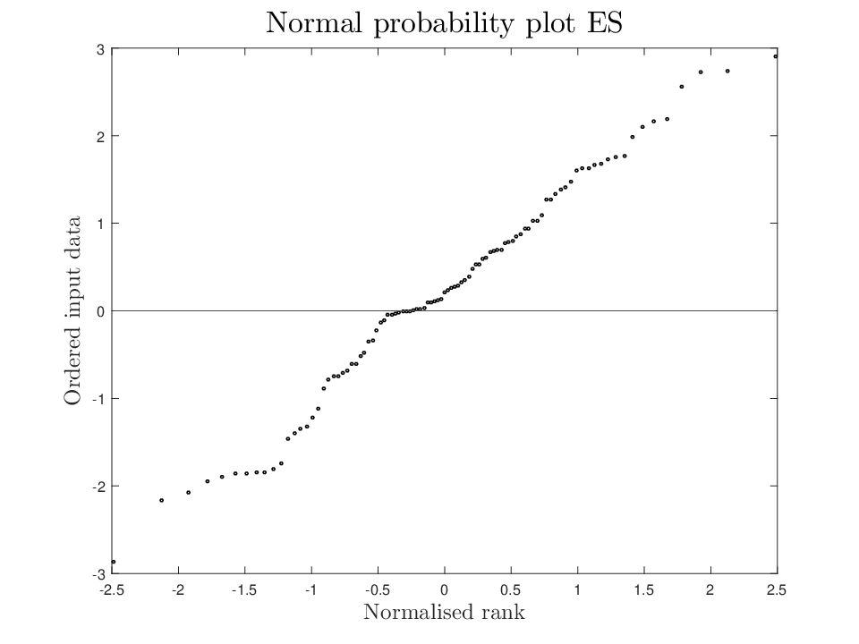
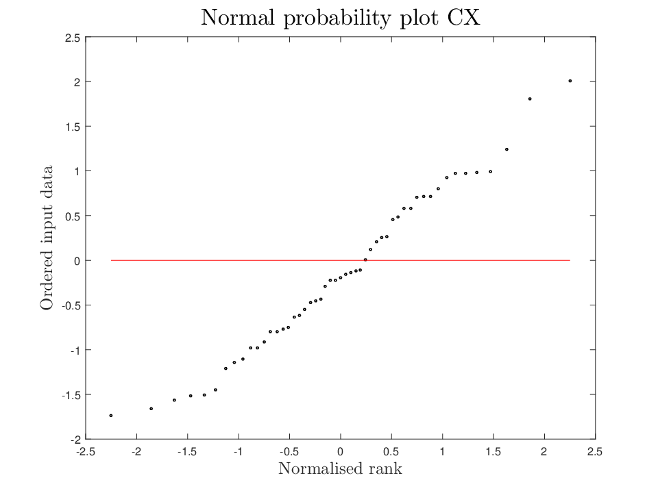
To extract a p-value for each input set of observations (sample data), the former test makes use of the -statistic, which essentially represents an approximate measure of the linear correlation between two quantities plotted against one another: the ordered sample-data quantiles (on one axis) and the standard normal quantiles (on the other); this plot is generally known as ‘normal probability plot’ (which is the Q-Q plot for the normal distribution). If the sample data comprises independent observations, which have been sampled from one normal distribution , then the points on the normal probability plot are arranged along a straight line. The departure of this scatter plot from linearity is equivalent to the departure of the sample data from the normal distribution. The -statistic is valued in : the upper bound represents ideal normality (of the sample data), whereas the exact opposite.
On the other hand, the D’Agostino-Pearson test compares the sample skewness and excess kurtosis (i.e., the difference between the evaluated kurtosis and , which is the kurtosis of the normal distribution) to their expectation values (for the dimension of the sample-data array) and combines two relevant tests into one ‘omnibus’ test, featuring the -statistic: if the underlying distribution is the normal distribution , then is -distributed with DoFs. The authors of Ref. [52] explain: “By omnibus, we mean it [i.e., the test] is able to detect deviations from normality due to either skewness or kurtosis.”
The distribution of the standardised residuals of the joint fits of the ETH model to the tDB± is somewhat negatively-skewed; the skewness of the distribution varies little across the one hundred joint fits, between about and . The kurtosis of the distribution (which varies between about and ) is below the expectation value of [57]. However, these effects are insignificant at the default significance threshold of this project: the p-values of the Shapiro-Wilk normality test vary between about and . The D’Agostino-Pearson test results in even higher p-values, between about and . The distribution of the standardised residuals is slightly translated to the right (the arithmetic mean of the distribution varies little in the joint fits, between about and ), and it is broader than the standard normal distribution (the variance of the distribution varies between about and in the fits). The normal probability plot in case of the standardised residuals of the joint fit of the ETH model to the tDB± for the median of the distribution (see Section 3.1.4) is shown in Fig. 5.
On the other hand, the distribution of the standardised residuals of the exclusive fit of the ETH model to the tDB0 is somewhat positively-skewed; the skewness of the distribution comes out equal to about . The kurtosis of the distribution (which is equal to about ) is again below the expectation value of [57]. Once again, these effects are insignificant at the default significance threshold of this project: the p-value of the Shapiro-Wilk normality test comes out equal to . The D’Agostino-Pearson test results in a higher p-value, about . The distribution of the standardised residuals is slightly translated to the left (the arithmetic mean of the distribution is equal to about ), and it is slightly narrower than the standard normal distribution (the variance of the distribution comes out equal to ). The normal probability plot in case of the standardised residuals of the exclusive fit of the ETH model to the tDB0 is shown in Fig. 6.
At the end of the day, there is no significant evidence of non-normality in the results of the tests of the fitted values of the standardised residuals . It must be borne in mind that the results of this section correspond to tests for normality, i.e., whether or not the standardised residuals have been sampled from one normal distribution , without regard to the and values. Ideally, these results follow the standard normal distribution , which - predominantly due to the effects in the tDB+, addressed at the end of Section 3.1.1 - can hardly be the case in the joint fits of the ETH model to the tDB±.
3.3 Predictions
As explained in Section 2.1, the analysis of the tDB0 using the ETH model is technically not a PSA, in that the two isospin amplitudes and cannot be determined from that analysis reliably; only their difference can. Evidently, any predictions (for the various quantities entering the low-energy interaction), obtained from such an analysis, make sense only if they relate to quantities which are associated with the CX reaction: for instance, the isovector scattering length , the isovector scattering volumes and , and the scattering amplitude . To be able to carry out a PSA of the tDB0, one must also involve data which can lead to the reliable determination of (at least) one of the two isospin amplitudes. This is why joint fits to the tDB+ and the tDB0 were pursued in the works of the recent past. Evidently, the PSA of the tDB0 was forfeited in this study, in order to enable the ‘clean’ determination of the scattering amplitude , i.e., without any involvement of measurements other than those contained in the tDB0.
3.3.1 phase shifts
The predictions for the - and -wave phase shifts, obtained from the PSA of the tDB±, are given in Table 8; they are also shown in Figs. 10-15, along with the XP15 solution [46], including (wherever available) the five single-energy values of that solution for MeV. Although the XP15 phase shifts are not accompanied by uncertainties 88 8 Due to the overconstrained fits, not even tentative/working uncertainties are published in the phase-shift solutions obtained from analyses using dispersion relations. Only the single-energy phase shifts of the XP15 solution (wherever available) are accompanied by realistic uncertainties., there can be no doubt that they do not match well the phase-shift solution of this work: the two sets of values remain well apart from one another in the low-energy region, converging only in the vicinity of the upper bound of this project. Of course, the differences between the two solutions are aggravated by the absence of (meaningful) uncertainties on the part of the XP15 solution.
The values of the two - and the four -wave phase shifts (in degrees), obtained in this study from the PSA of the tDB±.
| (MeV) | () | () | () | () | () | () |
|---|---|---|---|---|---|---|
3.3.2 Low-energy constants of the interaction
At low energy, the hadronic part of the scattering amplitude may safely be confined to - and -wave contributions, see Ref. [58], pp. 17–18. Introducing the isospin of the pion as and that of the nucleon as (and using natural units for the sake of brevity), may be put in the form:
| (4) |
where is (double) the spin of the nucleon; and are the CM -momenta of the incoming and outgoing pions, respectively. The third term on the rhs of this equation is the no-spin-flip -wave part of the scattering amplitude, whereas the fourth (i.e., the last) term is the spin-flip part.
Equation (4) defines the isoscalar (subscript ) and isovector (subscript ) -wave scattering lengths ( and ) and -wave scattering volumes (, , , and ), which are related to the usual spin-isospin scattering lengths/volumes according to the transformations, e.g., see Eqs. (2.39) of Ref. [58].
| (5) |
Table 9 contains predictions for these quantities, obtained from the PSA of the tDB±. A few remarks are in order.
- •
There is no doubt that the inclusion in the DB- (for the first time, in the ZRH19 PSA [3]) of the two scattering lengths , extracted from the PSI measurements of the strong shift of the ground state in pionic hydrogen (see Table 1), leads to solutions with enhanced isoscalar components in the low-energy amplitude. Prior to this inclusion, the isoscalar scattering length used to come out small, close to (and not incompatible with) . There are two consequences of this ‘new’ reality. First, the scattering length tends to come out slightly less negative (in comparison with former PSAs). The second consequence concerns the estimates for the term: although the prediction, obtained in this work on the basis of the ETH model ( MeV), is in good agreement with the estimate obtained by the SAID group in 2002 [59], it significantly exceeds the result of Ref. [16]: the difference between the two values is (nearly entirely) due to the aforementioned ‘enhancement’ of the DB- in 2019. (Incidentally, Olsson set forth a pioneering scheme for evaluating the term over two decades ago, using only a few LECs of the low-energy interaction [60], see also Section 4.2.2 of Ref. [16]. Using Eq. (63) therein, one obtains from the LECs of Table 9: MeV. The estimate of this work for the isoscalar effective range , which is needed in the aforementioned evaluation, is .)
- •
The estimate for , fully corrected (for the scale-factor effects of Section 3.2.1), is in good agreement with the experimental results of Refs. [11, 28]. Of course, this is hardly surprising, given that (owing to their unprecedented precision) the two ‘experimental’ results act as ‘anchor points’ in the optimisation, forcing the solution to ‘gravitate’ towards their direction.
- •
The prediction for the scattering length of the CX reaction (i.e., for the quantity in Table 9), obtained from the PSA of the tDB±, is significantly less negative than the estimates of Table 1, obtained from the PSI measurements of the total decay width of the ground state in pionic hydrogen [8, 11]. This result is neither new nor surprising: as a matter of fact, it is one manifestation of what is outlined in Ref. [1] as the ‘low-energy enigma’.
Upper part: The isoscalar and isovector -wave scattering lengths (in and in fm) and -wave scattering volumes (in and in fm3), obtained from the PSA of the tDB±; these quantities are defined by Eq. (4). Middle part: the corresponding results for the spin-isospin quantities. Lower part: the predictions for the fully-corrected (for the scale-factor effects of Section 3.2.1) scattering lengths which are associated with the three low-energy processes (i.e., with the , ES, and CX reactions).
| Scattering length/volume | In (reciprocal) powers of | In powers of fm |
| Isoscalar-isovector scattering lengths and volumes | ||
| Spin-isospin scattering lengths and volumes | ||
| Fully-corrected scattering lengths associated with the physical processes | ||
Table 10 contains the predictions for the isovector scattering lengths and volumes, obtained from the exclusive fit of the ETH model to the tDB0. The differences between the corresponding entries of Tables 9 and 10 for the isovector scattering lengths and volumes are significant in all cases. A comparison between the fully-corrected result of Table 10 and the corresponding ‘experimental’ entry of Table 1 suggests that the scattering data of the tDB0 would rather favour a somewhat smaller value for the total decay width of the ground state in pionic hydrogen; to be specific, a value in the vicinity of meV.
The isovector -wave scattering length (in and in fm) and -wave scattering volumes (in and in fm3), obtained from the exclusive fit of the ETH model to the tDB0. The table also contains the fully-corrected (for the scale-factor effects of Section 3.2.1) scattering length associated with the CX reaction.
| Scattering length/volume | In (reciprocal) powers of | In powers of fm |
|---|---|---|
| Isovector scattering lengths and volumes | ||
| Fully-corrected scattering length of the CX reaction | ||
3.3.3 Reproduction of the absolute normalisation of the DB0 by the BLS±
The methodology, which is relevant to this part, was put forward in Ref. [34], and was first applied to the reproduction of the absolute normalisation of the DB0 in the ZRH17 PSA [3]. One first determines a set of predictions from the PSA of the tDB±, relating to the observables and to the corresponding values of the kinematical variables at which the actual measurements in the DB0 had been acquired. Predictions and measured data are subsequently compared. The amount, at which each set of predicted values must be floated in order that it optimally reproduces the corresponding dataset of the DB0, is determined; relevant to this part of the analysis are the free-floating scale factors of Eq. (20).
The extracted values for the datasets, which are associated with measurements of the DCS (this includes the TCS, as well as the coefficients in the Legendre expansion of the DCS 99 9 Being ratios of cross sections, the APs might not be equally sensitive to the effect under investigation in this section, i.e., to the violation of isospin invariance.), and their total uncertainties , i.e., the purely statistical uncertainties
(where the weights are defined in Appendix C) combined (quadratically) with the normalisation uncertainty of the dataset, are given in Table 15 and, plotted separately for the DCS, for the TCS, and for the coefficients in the Legendre expansion of the DCS, in Fig. 16. Not included in the figure (but given in the table) are the results for the four FITZGERALD86 datasets which had been freely floated in the optimisation, as well as the estimate for the BREITSCHOPF06 one-point dataset which had been removed at step (3) of the procedure of Section 2.3, see also Table 5. An interesting feature of Table 15 is that no dataset is labelled as having problematical shape; on the contrary, datasets are labelled as having problematical absolute normalisation.
Inspection of Fig. 16 leaves no doubt that the free-floating scale factors of the datasets in the tDB0 contain an appreciable amount of fluctuation. As the BLS± prediction is smooth, this fluctuation reflects the variation of the absolute normalisation of the datasets in the DB0. For the sake of example, the value for the FRLEŽ98 dataset comes out equal to . This dataset lies in-between three datasets with considerably smaller values, namely between the two ISENHOWER99 -MeV datasets and the MEKTEROVIĆ09 -MeV dataset. The results for the absolute normalisation of the two neighbouring datasets of DUCLOS73 ( and MeV) and that of the JIA08 -MeV dataset (both accompanied by large normalisation uncertainties), are compatible with the BLS±.
The exponential function
| (6) |
has been fitted to the values of Fig. 16. The fitted values of the parameters and , corrected for the quality of the fit (resulting in for DoFs), are equal to and MeV-1, respectively. Similar results had been obtained in the former analyses of the recent past [3], see Table 11, pointing to a significant discrepancy (between the DB0 and the corresponding BLS±) in the low-energy region.
The fitted values and uncertainties of the parameters and of the empirical exponential function of Eq. (6), which is used for modelling the energy dependence of the free-floating scale factors of the CX datasets, obtained from the reproduction of the DB0 by the BLS±. If the scale factors had come out as predicted by the PSA of the tDB±, then the parameter would have vanished.
| Year | (MeV-1) | |
|---|---|---|
| 2017 | ||
| 2019 | ||
| 2020 | ||
| This work |
Integrated between and MeV, this discrepancy between measured and predicted cross sections is equivalent to an effect at the level of or, naively converted into a relative difference (denoted as in Ref. [1]) between the two CX scattering amplitudes, of . Although, owing to the pronounced energy dependence of the effect, these percentages should not to be taken seriously, they nevertheless corroborate the mathematically-sound comparison, based on Eq. (2) and presented in the following section.
3.3.4 Test for the departure from the triangle identity
The objective in this section is to compare the real parts of two CX scattering amplitudes: the first, , represents the prediction obtained in this study from the PSA of the tDB±; the second, , is obtained from the exclusive fit of the ETH model to the tDB0.
According to Eq. (3) of Ref. [2], the real part of each partial-wave amplitude and the corresponding phase shift are linked via the expression:
Expressed in terms of the two isospin amplitudes, the partial-wave amplitudes of the CX reaction are given by the relation:
For the wave, one obtains:
| (7) |
Using Eqs. (3.3.2), the corresponding expressions for the no-spin-flip and for the spin-flip -wave parts of the CX scattering amplitude (respectively) read as:
| (8) |
| (9) |
The real parts of the amplitudes and are shown in Figs. 17-19, separately for the wave, and for the no-spin-flip and spin-flip -wave parts. It was over twenty-five years ago when such a comparison was made, in the first report on the violation of isospin invariance in the interaction at low energy [61], see Figs. 1-3 therein. Shown in those figures was the energy dependence of the real parts of the three partial-wave amplitudes in the energy domain between and MeV: their difference in the wave was found to be nearly constant, evaluated in Ref. [61] to fm. Although the real part of the -wave CX scattering amplitude, obtained in this study from the PSA of the tDB±, seems to exhibit a more pronounced energy dependence (in comparison with the corresponding result of Ref. [61]), the estimate of this work for the difference (an average over the energy domain of Ref. [61]) is nearly unchanged: fm. A similar result was obtained in Ref. [2] using (as modelling option of the hadronic part of the interaction) the ETH parameterisation. As Fig. 17 indicates, the energy dependence of the difference between the real parts of the two -wave CX scattering amplitudes is pronounced in the low-energy region, decreasing with increasing energy. In comparison with the result of Ref. [2], the convergence of the two solutions evidently occurs above the upper bound of this project (i.e., above MeV).
3.3.5 Reproduction of the DCSs of the CHAOS Collaboration by the BLS±
This section examines the reproduction of the CHAOS DCSs [32], which amount to a prodigious datapoints, the largest (by far) contribution to the low-energy DB from a single experimental campaign (thus far). After two exclusive analyses of these measurements a few years ago [33, 34], it was decided to exclude them from the DB of this project; although the subject was revisited in subsequent PSAs [3], that decision remained unchanged.
After following the recommendation by two members of the CHAOS Collaboration [62] to avoid segmenting their data, the twelve original datasets (six for each ES reaction 1010 10 For both reactions, the CHAOS data contain two datasets at MeV: the second set (in each reaction) was obtained after the target was rotated; to distinguish between the two target configurations for the -MeV datasets, the ones with rotated target are labelled ‘(rot.)’.) were submitted to the tests of the overall reproduction, of the reproduction of the shape, and of the reproduction of the absolute normalisation, as these tests are set forth at the end of Appendix C. The following conclusions were drawn.
- •
None of the datasets can be accounted for. The best-reproduced dataset was the one at the lowest energy ( MeV): the p-value of its reproduction came out equal to a mere .
- •
In all cases, the inability to reproduce the datasets may be imputed to the shape of the angular distribution of the DCS. (The absolute normalisation of the -MeV dataset also emerges as problematical.)
- •
Apart from the -MeV dataset, the shape of the angular distribution of the ES measurements is also problematical, though in a less pronounced way than it is in case of the data.
- •
If one pays no heed to the problematical shape of the angular distribution of these datasets and proceeds with the determination of a representative, so to speak 1111 11 Without doubt, given the problematical shape of the DCSs in both cases, the averages of this paragraph ought to be taken with a grain of salt., absolute normalisation of the data (e.g., by averaging the free-floating scale factors obtained with Eq. (20)), then the absolute normalisation of the datasets turns out to be between and ( confidence interval) above the bulk of the tDB+ (), whereas that of the ES datasets is (on average) between and ( confidence interval) below the absolute normalisation of the tDB- (); of course, the absolute normalisation of the tDB- is largely determined by the precise PSI measurements of in pionic hydrogen (which lead to the scattering length ). Although one might be tempted to conclude that the absolute normalisation of the CHAOS ES datasets does not match well the value of the scattering length , as this quantity emerges from the experimental investigation at the threshold, such a conclusion might be rash at this time 1212 12 Prior to the inclusion in the DB of this project of the two ‘experimental’ values of the scattering length , the extrapolation of the ES amplitude from the scattering region to the threshold invariably resulted in lower values than those extracted from the experiments on pionic hydrogen. In this respect, the (representative) absolute normalisation of the CHAOS ES datasets is not necessarily in conflict with that of the tDB-; it only appears to be, simply due to the large impact which the precise measurements at the threshold have on the optimisation, by ‘attracting’ the fitted values of the ES amplitude in their direction. One consequence of the inclusion of the two experimental results in the DB of this project is that the reproduction of the CHAOS ES measurements by the BLS± deteriorated..
The reproduction of the CHAOS DCSs by the BLS± of this work is shown in Figs. 23 and 24. As a sum over the contributions of Eq. (C), one obtains the (reproduction) values of for datapoints and for ES datapoints: the largeness of these results demonstrates beyond doubt that the CHAOS DCSs (original datasets) cannot be reproduced by the BLS± of this work (as well). In comparison with former works in this project (e.g., with the ZRH19 PSA), the quality of the reproduction of these datasets slightly deteriorated due to one additional reason: the predictions are now accompanied by somewhat smaller uncertainties, emanating from the narrower distribution from which the parameter is currently sampled for the joint fits of the ETH model to the tDB±.
In Refs. [33, 34], it was argued that the segmentation of the original datasets of the CHAOS Collaboration, into forward-, intermediate-, and backward-angle data, is dictated by the procedure which had led to the reported results in Ref. [32]. In fact, the CHAOS DCSs had been inserted into (and can be found in) the SAID DB in the form of segmented datasets. Of course, in comparison with the original ones, the segmented datasets are expected to be accounted for in a more satisfactory manner (regardless of the analysis method), the reason being that the segmented parts of each original dataset are floated independently of each other. As contribution of the CHAOS DCSs to the of their fit, the SAID group report a total value of for datapoints ( for the and for the ES datasets); one datapoint of the -MeV dataset at intermediate angles has been removed from the input by the SAID analysts. Therefore, even the segmented datasets are poorly described by the WI08 solution 1313 13 Using the SAID Analysis Program [7], I was not able to obtain information about the description of the data on the basis of the more recent solution XP15. The selection of the ‘current’ solution in the user interface brings up the details about the description which is obtained on the basis of the former solution WI08 [63], the remaining two options involving results corresponding to two outdated Karlsruhe analyses of the 1980s. However, the chances are that the difference in the description of the CHAOS DCSs between the WI08 and the XP15 solutions is (at worst) negligible.: when considering the description of the segmented datasets by the WI08 solution, p-values are below the default significance threshold of this project.
The segmented datasets were also analysed in this study. The conclusion is that the following datasets cannot be reproduced:
- •
the observations at , , , , and (rot.) MeV at forward angles (i.e., five of the six datasets involving measurements in the Coulomb peak) and
- •
the observations at , , , and (rot.) MeV at intermediate angles.
In three cases, the problems are due to problematical shape; in six, due to problematical absolute normalisation. From the ES measurements, both -MeV datasets, as well as the - and (rot.)-MeV datasets at intermediate/backward angles, are poorly reproduced (all due to problematical shape). Using the segmented datasets, the reproduction values were obtained (sums over the contributions given in Eq. (C)): for datapoints and for ES datapoints. Table 16 provides the important details about the reproduction of the CHAOS DCSs, both of the original, as well as of the segmented datasets.
It would be instructive to enquire further into the description by the WI08 solution of the nine (segmented) datasets, which cannot be reproduced by the BLS± of this work. The sum of the relevant values, directly copied from the output of the SAID Analysis Program, is equal to . As datapoints are contained within these sets, the reduced value, corresponding to the description of these datasets by the WI08 solution, is equal to about , hence poorer by comparison with the average description of the CHAOS DCSs by that solution.
Further examination might be revealing as far as the identification of the source of the observed discrepancies is concerned. One of the possibilities is to analyse the results obtained in the three angular intervals of the segmented datasets (i.e., forward, intermediate, and backward). The reproduction of the data at backward angles by the BLS± of this work leads to for datapoints. This result is very satisfactory 1414 14 As the hadronic part of the interaction dominates at backward angles (the direct EM contributions vanish at rad), this result suggests that the hadronic component of the amplitudes, emerging from the DCSs of the CHAOS Collaboration, can be accounted for by the BLS± of this work! and may be used as reference in the -tests (see Ref. [64], pp. 116-117), which will aim at assessing the quality of the reproduction of the datasets at forward and at intermediate angles relative to the reproduction at backward angles. In the former case, for datapoints. Using the reduced value of the datasets at backward angles as reference, one obtains for the -statistic: for and DoFs, resulting in the p-value of about and (thus) suggesting a substantial deterioration in the reproduction of the datasets at forward angles (with respect to that of the measurements at backward ones); visual inspection of Fig. 23 confirms this result. The corresponding p-value for the datasets at intermediate angles comes out equal to about , hence indicative of a (milder) deterioration in the reproduction of the data as one shifts from backward to intermediate angles. Evidently, the quality of the reproduction of the CHAOS DCSs steadily deteriorates as one moves from to rad. It must be mentioned that the description of the data by the WI08 solution is equally poor (or, for those who see the glass half full, equally good) in all three angular intervals (forward, intermediate, and backward): their reduced values for the datasets range between and , thus providing support for the scenario of a general underestimation of the uncertainties on the part of the CHAOS Collaboration regardless of the angular domain. In any case, the output of the SAID Analysis Program [7] provides no evidence of significant deterioration of the description of the segmented datasets by the WI08 solution in any of the aforementioned angular intervals. This is an interesting difference between the BLS± of this work and the WI08 solution.
The problematical nature of these DCSs may already be revealed by examining the experimental reports of the CHAOS Collaboration. For instance, upon inspection of the single-energy phase shifts obtained from these data (see Table 6.1 of Denz’s dissertation and Fig. 4 of their main publication [32]), one cannot but feel rather uneasy about the quoted values. Of course, it is true that single-energy phase-shift solutions cannot exhibit the smoothness of the results obtained when the energy dependence of the phase shifts is modelled by means of continuous functions. Having said that, the estimate for the phase shift (, no uncertainty has been quoted) in Table 6.1 of the dissertation, at MeV, is wrong by about ; the largest of the -wave phase shifts at low energy, , is itself about at that energy! At MeV, the WI08 result [63] for () generally agrees with the values reported in this programme over time, see also Table 8. It is my thesis that this discrepancy alone ought to have sufficed in providing the motivation for the thorough re-examination of the CHAOS DCSs.
Due to the reasons which have been laid out in this section, I cannot recommend the use of the CHAOS DCSs in analyses of the low-energy data, in particular in sensitive ones, as (for the sake of example) are those which aim at evaluating the term [65]. Unless these measurements are revised in the light of Refs. [3, 33, 34], as well as of this work, I see no alternative to excluding the CHAOS DCSs from the PSAs of this project.
It would be constructive if the exclusive description of the CHAOS DCSs were pursued by means of a different methodology. As the beam energy of these datasets is low, an investigation of their description within the framework of Chiral-Perturbation Theory, e.g., using the method of Ref. [66], or following the method of Ref. [67] should be possible. Alternatively, the reproduction of these datasets could be examined on the basis of available results, obtained from the remaining data in the aforementioned schemes.
I shall conclude this section with a few words about the inclusion of the CHAOS DCSs in the SAID DB. Provided that their number remains reasonably small, the methodology, which is followed in the analyses of the ETH project, can handle the presence of outliers in the DBs, both in terms of the shape as well as of the absolute normalisation of the datasets. However, the breakdown point 1515 15 The breakdown point of an analysis is the fraction of discrepant data it can handle before it starts to produce erroneous results. The breakdown point is an increasing function of the level of robustness of the analysis method. of the approach is expected to be low, presumably not exceeding about . Given the restriction of the DBs to low energy, the inclusion of the CHAOS DCSs in the DB± of this project cannot be considered ‘small’ by any means; the addition of datapoints to a DB, which contains measurements, makes sense if the existing and the added parts are not in conflict. Figures 23 and 24 amply demonstrate that this is hardly the case. On the other hand, the SAID group could afford to add the entirety of the CHAOS DCSs to their DBs because they (i.e., their 2004 DBs) already contained tens of thousands of datapoints (namely all measurements up to the few-GeV region, barring the measurements of the PTCS/TNCS/TCS and those at the threshold); their sensitivity to the treatment of a few hundred unscreened measurements is certainly lower than it would have been in case of this project.
4 Conclusions and discussion
Carried out in this study is an improved analysis of the measurements of the three pion-nucleon () reactions which can be subjected to experimental investigation at low energy (pion laboratory kinetic energy MeV), i.e., of the two elastic-scattering (ES) processes and of the charge-exchange (CX) reaction .
There are a number of differences to the works of the recent past (which can be found online as versions of Ref. [3]). The most important modification relates to the analysis procedure. The old analysis procedure, which had been applied to several works during the past decade, can be found in Section 3.1 of Ref. [2]. The new analysis procedure, which is detailed in Section 2.3 of this study, introduces a number of improvements, which (hopefully) make its application more straightforward and comprehensible to the (non-expert) reader.
- a)
The joint fits of the ETH model to the measurements of the and CX reactions, which had been carried out in order that a second phase-shift solution (one involving the CX data) be reliably determined, will be replaced (from now on) by exclusive fits of that model to the low-energy database (DB) of the CX reaction. This development became possible after suppressing (whenever the CX measurements are submitted to the optimisation) the contributions to the partial-wave amplitudes of the ETH model which originate from the scalar-isoscalar -channel Feynman diagram, see Fig. 1 (left graph, upper part).
The main solution, obtained with the ETH model, will continue to be the one associated with the phase-shift analysis (PSA) of the measurements of the ES reactions. The second solution will be obtained from the exclusive fit of the ETH model to the low-energy CX data. As a result, the extraction of the CX scattering amplitude from the experimental data of that reaction will be ‘clean’, in the sense that it will no longer rely on the involvement of the experimental data of a second process. As the two types of fits now involve input DBs which have no commonality, the two solutions, obtained from these fits, are independent of one another. - b)
The modifications of case (a) above enabled the reliable evaluation of the popular measure of the violation of isospin invariance of Eq. (2), in the entire low-energy region, separately for the wave, as well as for the no-spin-flip and spin-flip -wave parts of the scattering amplitude, see Figs. 17-22.
- c)
For the first time in several years, the DB of the low-energy measurements has been enhanced in this work with the inclusion of sixteen datapoints, which had been available for a long time but had not been used thus far (on account of the reasons which can be found in Section 2.2), namely of the differential cross sections (DCSs) of two experiments of the late 1970s [4, 5], as well as of the three-point dataset of Ref. [6], which corresponds to measurements of the CX DCS at MeV. One additional datapoint, the scattering length , as this entry emerges from the recent publication of the total decay width of the ground state in pionic hydrogen by the Pionic Hydrogen Collaboration [8] - and the application of the electromagnetic (EM) corrections of Ref. [29], was appended to the DB of the CX reaction.
- d)
Apart from the physical properties of a few higher baryon resonances [18], as well as of three scalar-isoscalar and one vector-isovector mesons [19], needed in order to determine the (inessential) contributions from these states to the partial-wave amplitudes of the ETH model, the values of the physical constants have been fixed in this analysis from the recent compilation of the Particle-Data Group [14].
After the application of the four steps of the first phase of the new analysis procedure, entries (of the DoFs of the new initial DB of this project, see Table 2) were identified as outliers and were removed from the DBs, see Tables 3-5. In this manner, three truncated DBs (tDBs, see the notation at the end of Section 1) were obtained, which were submitted to further analysis using the ETH model, see the two last steps of the analysis procedure described in Section 2.3.
The optimisation of the description of the ES measurements (step (5) of Section 2.3), i.e., of the tDB±, was achieved on the basis of the numerical minimisation provided by the MINUIT software package [68] of the CERN library (FORTRAN version), using the Arndt-Roper formula [13] to obtain the contributions of the datasets to the overall , see Appendix A. The PSA of the tDB± comprises the results of one hundred joint fits to the same data, each fit being carried out at one value of the model parameter , which is associated with the effective range of the scalar-isoscalar part of the interaction: the values were randomly generated in normal distribution, in accordance with the result of Ref. [19]. The optimal values of the parameters of the ETH model, taking all uncertainties into account (as well as the variation), can be found (corrected for the quality of the fits via the application of the Birge factor [20]) in Table 6. The most important of these parameters is the pseudoscalar coupling constant , which comes out equal to . Converted into a result for the pseudovector coupling constant , to be identified with the charged-pion coupling constant of Ref. [50], this estimate translates into:
This result is in good agreement with the findings of Refs. [50, 69], as well as with the values extracted in the analyses of the SAID group over time, see Ref. [50] for details.
The results of the PSA of the tDB± lead to predictions for the phase shifts (Section 3.3.1, Figs. 10-15), for the low-energy constants (LECs) of the interaction (Section 3.3.2), etc. In addition, they can be used to derive estimates for all measurable quantities, for all three low-energy reactions. Two such sets of predictions were obtained in this work: the first was used in the assessment of the quality of the reproduction of the absolute normalisation of the DB0 (Section 3.3.3, Table 15, Fig. 16); the second was used in the assessment of the quality of the reproduction of the DCSs of the CHAOS Collaboration, which are not included in the DB of this project (Section 3.3.5, Table 16, Figs. 23 and 24). The interest in the former case relates to the tests of the triangle identity of Eq. (1), a relation which is fulfilled if the isospin invariance holds in the low-energy interaction. The interest in the latter case relates to providing an explanation for the inability to account for the DCSs of the Chaos Collaboration within the ETH project.
The exclusive fit of the ETH model to the CX data cannot determine both isospin amplitudes, and ; only their difference can reliably be determined from that fit. Consequently, the analysis of the tDB0 using the ETH model is technically not a PSA, which implies that it cannot lead to a reliable phase-shift solution. From the exclusive fit of the ETH model to the tDB0, only quantities associated with the CX reaction can be estimated, e.g., the isovector scattering lengths and volumes (see end of Section 3.3.2), as well as the scattering amplitude .
Cutkosky introduced in 1979 the Quantum-Mechanical (QM) admixture of the and the mesons as a potential mechanism for the violation of isospin invariance in the interaction [23]; affected by this mechanism is the CX reaction. The consequences of fitting an isospin-invariant model (such as the ETH model is) to measurements which presumably contain isospin-breaking effects have been touched upon at the beginning of Section 2.1.1. Provided that the QM admixture of the and the mesons is the dominant means by which the violation of isospin invariance occurs in the CX reaction, the creation of a complete hadronic model of that reaction necessitates the addition of the contributions from the Feynman diagrams of Fig. 4 to those of Fig. 1. As the five-parameter fit of the ETH model to the tDB0 verges on the border of the realms of possibility, any additional parameters (i.e., introduced by the Feynman diagrams of Fig. 4) ought to be fixed from external sources; unfortunately, the coupling constants and the vertex factors of the meson are not well known (if at all) at this time, see end of Section 4.1 of Ref. [1] for comments on the coupling constant . Therefore, one is left with only one option: to fit the ETH model, in its current isospin-invariant form, to the data and hope that the optimisation of the description of the tDB0 will return a reasonable for the NDF of the fit and no significant effects in the distribution of the fitted values of the scale factor . This was the strategy in this study (step (6) of Section 2.3), and it seems to have been successful on both accounts. Having said that, the fitted values of the parameters of the ETH model, as they emerge from this exclusive fit, are bound to be effective, as they certainly contain contributions which are (currently) beyond the modelling of the hadronic part of the CX reaction by the ETH model. The differences between the two sets of results (i.e., between those obtained from the PSA of the tDB± and the ones resulting from the exclusive fit of the ETH model to the tDB0) are significant for all model parameters, see Table 6.
In Section 3.3.3, the reproduction of the absolute normalisation of the DB0 was investigated on the basis of the results obtained from the PSA of the tDB±. Figure 16 demonstrates that most of the CX datasets have an absolute normalisation which exceeds the prediction obtained from the ES data. This result is not new; similar plots have been obtained in all analyses of the low-energy data within the ETH project during the past two decades, resulting in a significant overall discrepancy between the two CX scattering amplitudes, i.e., between
- •
the amplitude , which is reconstructed from the ES data, i.e., obtained from the PSA of the tDB± via Eq. (1), and
- •
the amplitude , which is obtained from the exclusive fit of the ETH model to the tDB0.
Integrated over the entire energy domain of this project, this discrepancy amounts to ; the corresponding results, obtained in the 2019 and 2020 PSAs of this project, were equal to and , respectively. However, given the pronounced energy dependence of the effect, it must not be forgotten that the quantity serves as an overall measure of the discrepancy at low energy; unlike the symmetrised relative difference between the two amplitudes, see Eq. (2), neither does it convey information about the energy dependence of the effect, nor can it reveal the source of the effect (i.e., the partial wave which is predominantly affected).
As aforementioned, the two amplitudes and emerge in this study from independent observations for the first time in years (in fact, since 1997 [12]); therefore, the results of their comparison are expected to be reliable. Separate comparisons of the energy dependence of these amplitudes are shown: in Fig. 17 for the wave; in Fig. 18 for the no-spin-flip -wave part; and in Fig. 19 for the spin-flip -wave part. The quantity is also shown in Figs. 20-22. Inspection of these figures suggests that significant effects can be established in the wave and in the no-spin-flip -wave part of the scattering amplitude; less significant effects can be observed in the spin-flip -wave part. These findings generally agree with the results of Refs. [12, 61]: in itself, this is quite remarkable, given that both studies had been based on a small fraction of the DB0 of this work.
Aiming at providing an explanation for the departure of the quantity from , three possibilities (or their combination) have been introduced and thoroughly discussed in Ref. [1], see Sections 5.1-5.3 therein; there is no need to repeat the arguments in this study. To summarise, the discrepancy may be attributable to:
- •
systematic effects in the absolute normalisation of the bulk of the low-energy data,
- •
substantial residual contributions (i.e., at present not included) in the EM corrections (which are applied to the data in order that the hadronic quantities be extracted), and
- •
the violation of isospin invariance in the interaction well beyond the expectations of Chiral-Perturbation Theory [70].
I should like to remind the interested reader that predictions for the usual observables (DCS, AP, PTCS, TNCS, and TCS) for the three low-energy reactions are simple to obtain, free of charge, and available within one week of the request date. Unlike the results obtained from dispersion relations, the predictions obtained within the ETH project are accompanied by uncertainties which reflect the statistical and systematic variation of the experimental data.
References
- [1] E. Matsinos, ‘What has been learnt from the analysis of the low-energy pion-nucleon data during the past three decades?’, arXiv:2205.02899 [nucl-th]. DOI: 10.48550/arXiv.2205.02899
- [2] E. Matsinos, ‘Low-energy parameterisations of the pion-nucleon phase shifts’, arXiv:2205.15604 [nucl-th]. DOI: 10.48550/arXiv.2205.15604
- [3] E. Matsinos, G. Rasche, ‘Update of the phase-shift analysis of the low-energy data’, arXiv:1706.05524 [nucl-th]. DOI: 10.48550/arXiv.1706.05524
- [4] M.A. Moinester et al., ‘Elastic scattering of positive pions on 12C at MeV’, Phys. Rev. C 18, 2678 (1978). DOI: 10.1103/PhysRevC.18.2678
- [5] M. Blecher et al., ‘Positive pion-nucleus elastic scattering at MeV’, Phys. Rev. C 20, 1884 (1979). DOI: 10.1103/PhysRevC.20.1884
- [6] J.L. Ullmann et al., ‘Pion single charge exchange on 14C from to MeV’, Phys. Rev. C 33, 2092 (1986). DOI: 10.1103/PhysRevC.33.2092
- [7] SAID Analysis Program: gwdac.phys.gwu.edu
- [8] A. Hirtl et al., ‘Redetermination of the strong-interaction width in pionic hydrogen’, Eur. Phys. J. A 57, 70 (2021). DOI: 10.1140/epja/s10050-021-00387-x
- [9]
D. Sigg et al., ‘Strong interaction shift and width of the level in pionic hydrogen’, Phys. Rev. Lett. 75, 3245 (1995).
DOI: 10.1103/PhysRevLett.75.3245 - [10] D. Sigg et al., ‘The strong interaction shift and width of the ground state of pionic hydrogen’, Nucl. Phys. A 609, 269 (1996); see also Erratum: Nucl. Phys. A 617, 526 (1997). DOI: 10.1016/S0375-9474(96)00280-1, 10.1016/S0375-9474(97)00135-8
- [11] H.-Ch. Schröder et al., ‘Determination of the scattering lengths from pionic hydrogen’, Phys. Lett. B 469, 25 (1999); H.-Ch. Schröder et al., ‘The pion-nucleon scattering lengths from pionic hydrogen and deuterium’, Eur. Phys. J. C 21, 473 (2001). DOI: 10.1016/S0370-2693(99)01237-X, 10.1007/s100520100754
- [12] E. Matsinos, ‘Isospin violation in the system at low energy’, Phys. Rev. C 56, 3014 (1997). DOI: 10.1103/PhysRevC.56.3014
- [13] R.A. Arndt, L.D. Roper, ‘The use of partial-wave representations in the planning of scattering measurements. Application to MeV scattering’, Nucl. Phys. B 50, 285 (1972). DOI: 10.1016/S0550-3213(72)80019-1
- [14] R.L. Workman et al. (Particle Data Group), ‘The Review of Particle Physics (2022)’, Prog. Theor. Exp. Phys. 2022, 083C01 (2022).
- [15] N. Fettes, E. Matsinos, ‘Analysis of recent low-energy differential cross-section measurements’, Phys. Rev. C 55, 464 (1997). DOI: 10.1103/PhysRevC.55.464
- [16]
E. Matsinos, G. Rasche, ‘Aspects of the ETH model of the pion-nucleon interaction’, Nucl. Phys. A 927, 147 (2014).
DOI: 10.1016/j.nuclphysa.2014.04.021 - [17] P.F.A. Goudsmit, H.J. Leisi, E. Matsinos, B.L. Birbrair, A.B. Gridnev, ‘The extended tree-level model of the pion-nucleon interaction’, Nucl. Phys. A 575, 673 (1994). DOI: 10.1016/0375-9474(94)90162-7
- [18] E. Matsinos, ‘Determination of the masses and decay widths of the well-established and baryon resonances below GeV’, arXiv:2008.06919 [hep-ph]. DOI: 10.48550/arXiv.2008.06919
- [19] E. Matsinos, ‘Determination of the masses and decay widths of the scalar-isoscalar and vector-isovector mesons below GeV’, arXiv:2007.13130 [hep-ph]. DOI: 10.48550/arXiv.2007.13130
- [20] R.T. Birge, ‘The calculation of errors by the method of least squares’, Phys. Rev. 40, 207 (1932). DOI: 10.1103/PhysRev.40.207
- [21] E. Matsinos, W.S. Woolcock, G.C. Oades, G. Rasche, A. Gashi, ‘Phase-shift analysis of low-energy elastic-scattering data’, Nucl. Phys. A 778, 95 (2006). DOI: 10.1016/j.nuclphysa.2006.07.040
- [22] E. Matsinos, ‘The contribution of the interference to the violation of the isospin invariance in the system’, arXiv:1804.09344 [nucl-th]. DOI: 10.48550/arXiv.1804.09344
- [23] R.E. Cutkosky, ‘Isospin violation in scattering from mixing’, Phys. Lett. B 88, 339 (1979). DOI: 10.1016/0370-2693(79)90482-9
- [24] P.Y. Bertin et al., ‘ scattering below MeV’, Nucl. Phys. B 106, 341 (1976). DOI: 10.1016/0550-3213(76)90383-7
- [25] P.J. Bussey et al., ‘ elastic scattering from to MeV’, Nucl. Phys. B 58, 363 (1973). DOI: 10.1016/0550-3213(73)90589-0
- [26] S. Deser, M.L. Goldberger, K. Baumann, W. Thirring, ‘Energy level displacements in pi-mesonic atoms’, Phys. Rev. 96, 774 (1954). DOI: 10.1103/PhysRev.96.774
- [27] T.L. Trueman, ‘Energy level shifts in atomic states of strongly-interacting particles’, Nucl. Phys. 26, 57 (1961). DOI: 10.1016/0029-5582(61)90115-8
- [28] M. Hennebach et al., ‘Hadronic shift in pionic hydrogen’, Eur. Phys. J. A 50 (2014) 190; see also Erratum: Eur. Phys. J. A 55, 24 (2019). DOI: 10.1140/epja/i2014-14190-x, 10.1140/epja/i2019-12710-x
- [29] G.C. Oades, G. Rasche, W.S. Woolcock, E. Matsinos, A. Gashi, ‘Determination of the -wave pion-nucleon threshold scattering parameters from the results of experiments on pionic hydrogen’, Nucl. Phys. A 794, 73 (2007). DOI: 10.1016/j.nuclphysa.2007.07.007
- [30] B. Tromborg, S. Waldestrøm, I. Øverbø, ‘Electromagnetic corrections to scattering’, Phys. Rev. D 15, 725 (1977). DOI: 10.1103/PhysRevD.15.725
- [31] R. Meier et al., ‘Low energy analyzing powers in pion-proton elastic scattering’, Phys. Lett. B 588, 155 (2004). DOI: 10.1016/j.physletb.2004.02.071
- [32]
H. Denz et al., ‘ differential cross sections at low energy’, Phys. Lett. B 633, 209 (2006); H. Denz, Ph.D. dissertation, Tübingen University, 2004. Available from
publikationen.uni-tuebingen.de/xmlui/handle/10900/48622.
DOI: 10.1016/j.physletb.2005.12.017 - [33] E. Matsinos, G. Rasche, ‘Analysis of the low-energy differential cross sections of the CHAOS Collaboration’, Nucl. Phys. A 903, 65 (2013). DOI: 10.1016/j.nuclphysa.2012.12.129
- [34] E. Matsinos, G. Rasche, ‘New analysis of the low-energy differential cross sections of the CHAOS Collaboration’, Int. J. Mod. Phys. E 24, 1550050 (2015). DOI: 10.1142/S0218301315500500
- [35] E.G. Auld et al., ‘ scattering at MeV’, Can. J. Phys. 57, 73 (1979). DOI: 10.1139/p79-008
- [36] E. Friedman, ‘Partial-total cross sections’, Newsl. 15, 37 (1999). Available from gwdac.phys.gwu.edu
- [37] A.A. Carter, J.R. Williams, D.V. Bugg, P.J. Bussey, D.R. Dance, ‘The total cross sections for pion-proton scattering between MeV and MeV’, Nucl. Phys. B 26, 445 (1971). DOI: 10.1016/0550-3213(71)90188-X
- [38] E. Pedroni et al., ‘A study of charge independence and symmetry from and total cross sections on hydrogen and deuterium near the resonance’, Nucl. Phys. A 300, 321 (1978). DOI: 10.1016/0375-9474(78)96136-5
- [39] M.E. Sevior et al., ‘Analyzing powers in elastic scattering from to MeV’, Phys. Rev. C 40, 2780 (1989). DOI: 10.1103/PhysRevC.40.2780
- [40] J. Duclos et al., ‘A measurement of the pion-nucleon charge-exchange reaction at , and MeV’, Phys. Lett. B 43, 245 (1973). DOI: 10.1016/0370-2693(73)90280-3
- [41] M. Salomon, D.F. Measday, J-M. Poutissou, B.C. Robertson, ‘Radiative capture and charge exchange of negative pions on protons at and MeV’, Nucl. Phys. A 414, 493 (1984). DOI: 10.1016/0375-9474(84)90615-8
- [42] D.V. Bugg et al., ‘The charge-exchange cross sections between MeV and MeV’, Nucl. Phys. B 26, 588 (1971). DOI: 10.1016/0550-3213(71)90197-0
- [43] J. Breitschopf et al., ‘Pionic charge exchange on the proton from to MeV’, Phys. Lett. B 639, 424 (2006). DOI: 10.1016/j.physletb.2006.07.009
- [44] B.J. Kriss et al., ‘Pion-proton integral cross section measurements’, Newsl. 12, 20 (1997). Available from gwdac.phys.gwu.edu; B.J. Kriss et al., ‘Pion-proton integral cross sections at to MeV’, Phys. Rev. C 59, 1480 (1999). DOI: 10.1103/PhysRevC.59.1480
- [45] A. Bagheri et al., ‘Reaction below the resonance’, Phys. Rev. C 38, 885 (1988). DOI: 10.1103/PhysRevC.38.885
- [46] R.L. Workman, R.A. Arndt, W.J. Briscoe, M.W. Paris, I.I. Strakovsky, ‘Parameterization dependence of -matrix poles and eigenphases from a fit to elastic scattering data’, Phys. Rev. C 86, 035202 (2012). DOI: 10.1103/PhysRevC.86.035202; I.G. Alekseev et al. (EPECUR Collaboration and GW INS Data Analysis Center), ‘High-precision measurements of elastic differential cross sections in the second resonance region’, Phys. Rev. C 91, 025205 (2015). DOI: 10.1103/PhysRevC.91.025205; A. Gridnev et al., ‘Search for narrow resonances in elastic scattering from the EPECUR experiment’, Phys. Rev. C 93, 062201(R) (2016). DOI: 10.1103/PhysRevC.93.062201
- [47] A. Gashi, E. Matsinos, G.C. Oades, G. Rasche, W.S. Woolcock, ‘Electromagnetic corrections to the phase shifts in low energy elastic scattering’, Nucl. Phys. A 686, 447 (2001). DOI: 10.1016/S0375-9474(00)00603-5
- [48] A. Gashi, E. Matsinos, G.C. Oades, G. Rasche, W.S. Woolcock, ‘Electromagnetic corrections for the analysis of low energy scattering data’, Nucl. Phys. A 686, 463 (2001). DOI: 10.1016/S0375-9474(00)00604-7
- [49] E. Matsinos, G. Rasche, ‘Systematic effects in the low-energy behavior of the current SAID solution for the pion-nucleon system’, Int. J. Mod. Phys. E 26, 1750002 (2017). DOI: 10.1142/S0218301317500021
- [50] E. Matsinos, ‘A brief history of the pion-nucleon coupling constant’, arXiv:1901.01204 [nucl-th]. DOI: 10.48550/arXiv.1901.01204
- [51] Available from https://math.mit.edu/ rmd/465/shapiro.pdf
- [52] R.B. D’Agostino, A. Belanger, R.B. D’Agostino Jr., ’A suggestion for using power and informative tests of normality’, Am. Stat. 44, 316 (1990). DOI: 10.2307/2684359
- [53] N. Mohd Razali, B. Yap, ‘Power comparisons of Shapiro-Wilk, Kolmogorov-Smirnov, Lilliefors and Anderson-Darling tests’, J. Stat. Model. Analytics 2, 21 (2011). ISBN: 9789673631575
- [54] S.S. Shapiro, M.B. Wilk, ‘An analysis of variance test for normality (complete samples)’, Biometrika 52, 591 (1965). DOI: 10.2307/2333709
- [55] J.P. Royston, ‘An extension of Shapiro and Wilk’s test for normality to large samples’, Appl. Statist. 31, 115 (1982). DOI: 10.2307/2347973; P. Royston, ‘Approximating the Shapiro-Wilk W-test for non-normality’, Stat. Comput. 2, 117 (1992). DOI: 10.1007/BF01891203; P. Royston, ‘A toolkit for testing for non-normality in complete and censored samples’, J. R. Stat. Soc., D: The Statistician 42, 37 (1993). DOI: 10.2307/2348109; J.P. Royston, ‘A Remark on Algorithm AS 181: The W-test for normality’, J. R. Stat. Soc., C: Appl. Stat. 44, 547 (1995). DOI: 10.2307/2986146
- [56] R. D’Agostino, E.S. Pearson, ‘Tests for departure from normality. Empirical results for the distributions of and ’, Biometrika 60, 613 (1973). DOI: 10.2307/2335012
- [57] E.S. Pearson, ‘I. Note on tests for normality’, Biometrika 22, 423 (1931). DOI: 10.1093/biomet/22.3-4.423
- [58] T.E.O. Ericson, W. Weise, ‘Pions and Nuclei’, Clarendon Press (1988). ISBN: 9780198520085
- [59] M.M. Pavan, R.A. Arndt, I.I. Strakovsky, R.L. Workman, ‘The pion-nucleon term is definitely large: results from a GWU analysis of scattering data’, Newslett. 16, 110 (2002). DOI: 10.48550/arXiv.hep-ph/0111066
- [60] M.G. Olsson, ‘The nucleon sigma term from threshold parameters’, Phys. Lett. B 482, 50 (2000). DOI: 10.1016/S0370-2693(00)00505-0
- [61]
W.R. Gibbs, Li Ai, W.B. Kaufmann, ‘Isospin breaking in low-energy pion-nucleon scattering’, Phys. Rev. Lett. 74, 3740 (1995).
DOI: 10.1103/PhysRevLett.74.3740 - [62] H. Denz, G.J. Wagner, private communication.
- [63] R.A. Arndt, W.J. Briscoe, I.I. Strakovsky, R.L. Workman, ‘Extended partial-wave analysis of scattering data’, Phys. Rev. C 74, 045205 (2006). DOI: 10.1103/PhysRevC.74.045205
- [64] M.R. Spiegel, J. Schiller, R.A. Srinivasan, ‘Probability and Statistics’, 4th edn., McGraw-Hill (2013). ISBN: 9780071795586
- [65] E. Matsinos, G. Rasche, ‘Comment on “Evaluation of the Pion-Nucleon Sigma Term from CHAOS Data”’, arXiv:1309.3469 [nucl-th]. DOI: 10.48550/arXiv.1309.3469
- [66]
J.M. Alarcón, J. Martin Camalich, J.A. Oller, ‘Improved description of the -scattering phenomenology at low energies in covariant baryon chiral perturbation theory’, Ann. Phys. 336, 413 (2013).
DOI: 10.1016/j.aop.2013.06.001 - [67] M. Hoferichter, J. Ruiz de Elvira, B. Kubis, Ulf-G. Meißner, ‘Roy-Steiner-equation analysis of pion-nucleon scattering’, Phys. Rep. 625, 1 (2016). DOI: 10.1016/j.physrep.2016.02.002
- [68] F. James, ‘MINUIT - Function Minimization and Error Analysis’, CERN Program Library Long Writeup D506.
- [69] P. Reinert, H. Krebs, E. Epelbaum, ‘Precision determination of pion-nucleon coupling constants using effective field theory’, Phys. Rev. Lett. 126, 092501 (2021). DOI: 10.1103/PhysRevLett.126.092501
- [70] M. Hoferichter, B. Kubis, Ulf-G. Meißner, ‘Isospin violation in low-energy pion-nucleon scattering revisited’, Nucl. Phys. A 833, 18 (2010). DOI: 10.1016/j.nuclphysa.2009.11.012
- [71] D. Binosi, L. Theußl, ‘JaxoDraw: A graphical user interface for drawing Feynman diagrams’, Comput. Phys. Commun. 161, 76 (2004). DOI: 10.1016/j.cpc.2004.05.001
- [72]
D. Binosi, J. Collins, C. Kaufhold, L. Theußl, ‘JaxoDraw: A graphical user interface for drawing Feynman diagrams. Version 2.0 release notes’, Comput. Phys. Commun. 180, 1709 (2009).
DOI: 10.1016/j.cpc.2009.02.020 - [73] J.A. Nelder, R. Mead, ‘A simplex method for function minimization’, Comput. J. 7, 308 (1965). DOI: 10.1093/comjnl/7.4.308
- [74] V.E. Johnson, ‘Revised standards for statistical evidence’, Proc. Natl. Acad. Sci. U.S.A. 110, 19313 (2013). DOI: 10.1073/pnas.1313476110
- [75] A. Gelman, C.P. Robert, ‘Revised evidence for statistical standards’, Proc. Natl. Acad. Sci. U.S.A. 111, E1933 (2014). DOI: 10.1073/pnas.1322995111
- [76] M. Abramowitz, I.A. Stegun, ‘Handbook of Mathematical Functions with Formulas, Graphs, and Mathematical Tables’, United States Department of Commerce, National Bureau of Standards (1972). ISBN: 9780318117300
- [77] W.H. Press, S.A. Teukolsky, W.T. Vetterling, B.P. Flannery, ‘Numerical Recipes: The Art of Scientific Computing’, 3rd edn., Cambridge University Press (2007). ISBN: 9780521880688
The datasets of the tDB+, i.e., of the DB+ after the application of step (1) of Section 2.3. The columns correspond to details about each dataset as follows: the identifier of the dataset in the DB of the ETH project; the pion laboratory kinetic energy (in MeV); the NDF of the dataset after the removal of any outliers; the fitted value of the scale factor of Eq. (11); the normalisation uncertainty (reported or assigned, see the introduction in Section 3); the value of of the description of the dataset in the fit, see Eq. (12); the corresponding p-value; and details in case of any removed DoFs. For freely-floated datasets, is identified with of Eq. (13).
| Identifier | p-value | Remarks | |||||
|---|---|---|---|---|---|---|---|
| DCSs | |||||||
| BERTIN76 | |||||||
| BERTIN76 | |||||||
| BERTIN76 | , | ||||||
| removed | |||||||
| BERTIN76 | |||||||
| BERTIN76 | |||||||
| BERTIN76 | removed | ||||||
| MOINESTER78 | |||||||
| AULD79 | |||||||
| BLECHER79 | |||||||
| RITCHIE83 | |||||||
| RITCHIE83 | |||||||
| RITCHIE83 | |||||||
| RITCHIE83 | |||||||
| FRANK83 | |||||||
| FRANK83 | |||||||
| FRANK83 | |||||||
| FRANK83 | |||||||
| BRACK86 | freely floated | ||||||
| BRACK86 | freely floated | ||||||
| BRACK86 | |||||||
| BRACK86 | |||||||
| BRACK88 | |||||||
Table 12 continued
| Identifier | p-value | Remarks | |||||
|---|---|---|---|---|---|---|---|
| BRACK88 | |||||||
| WIEDNER89 | |||||||
| BRACK90 | |||||||
| BRACK90 | |||||||
| BRACK95 | |||||||
| BRACK95 | |||||||
| JORAM95 | , | ||||||
| removed | |||||||
| JORAM95 | |||||||
| JORAM95 | removed | ||||||
| JORAM95 | , , | ||||||
| removed | |||||||
| APs | |||||||
| SEVIOR89 | |||||||
| WIESER96 | |||||||
| WIESER96 | |||||||
| MEIER04 | |||||||
| MEIER04 | , | ||||||
| MEIER04 | |||||||
| PTCSs | |||||||
| KRISS97 | |||||||
| KRISS97 | |||||||
| KRISS97 | |||||||
| KRISS97 | |||||||
| KRISS97 | |||||||
| KRISS97 | |||||||
| KRISS97 | |||||||
| KRISS97 | |||||||
| KRISS97 | |||||||
Table 12 continued
| Identifier | p-value | Remarks | |||||
|---|---|---|---|---|---|---|---|
| KRISS97 | |||||||
| KRISS97 | |||||||
| KRISS97 | |||||||
| KRISS97 | |||||||
| FRIEDMAN99 | |||||||
| FRIEDMAN99 | |||||||
| FRIEDMAN99 | |||||||
| FRIEDMAN99 | |||||||
| FRIEDMAN99 | |||||||
| FRIEDMAN99 | |||||||
| TNCSs | |||||||
| CARTER71 | |||||||
| CARTER71 | |||||||
| PEDRONI78 | |||||||
| PEDRONI78 | |||||||
| PEDRONI78 | |||||||
| PEDRONI78 | |||||||
The equivalent of Table 12 for the tDB-, i.e., for the DB- after the application of step (2) of Section 2.3.
| Identifier | p-value | Remarks | |||||
|---|---|---|---|---|---|---|---|
| DCSs | |||||||
| FRANK83 | |||||||
| FRANK83 | |||||||
| FRANK83 | |||||||
| FRANK83 | |||||||
| BRACK86 | |||||||
| BRACK86 | |||||||
| BRACK86 | |||||||
| BRACK86 | |||||||
| WIEDNER89 | removed, | ||||||
| freely floated | |||||||
| BRACK90 | |||||||
| BRACK90 | |||||||
| BRACK95 | |||||||
| BRACK95 | removed | ||||||
| JORAM95 | |||||||
| JORAM95 | |||||||
| JORAM95 | |||||||
| JORAM95 | |||||||
| JORAM95 | |||||||
| JORAM95 | |||||||
| JORAM95 | |||||||
| JORAM95 | |||||||
| JANOUSCH97 | |||||||
| JANOUSCH97 | |||||||
| JANOUSCH97 | |||||||
| JANOUSCH97 | |||||||
| JANOUSCH97 | |||||||
Table 13 continued
| Identifier | p-value | Remarks | |||||
|---|---|---|---|---|---|---|---|
| Scattering length from the strong shift of pionic hydrogen | |||||||
| SCHROEDER01 | |||||||
| HENNEBACH14 | |||||||
| APs | |||||||
| ALDER83 | |||||||
| SEVIOR89 | |||||||
| HOFMAN98 | |||||||
| PATTERSON02 | |||||||
| PATTERSON02 | |||||||
| PATTERSON02 | |||||||
| PATTERSON02 | |||||||
| PATTERSON02 | |||||||
| PATTERSON02 | |||||||
| MEIER04 | , | ||||||
The equivalent of Table 12 for the tDB0, i.e., for the DB0 after the application of step (3) of Section 2.3.
| Identifier | p-value | Remarks | |||||
|---|---|---|---|---|---|---|---|
| DCSs | |||||||
| DUCLOS73 | |||||||
| DUCLOS73 | |||||||
| DUCLOS73 | |||||||
| FITZGERALD86 | freely floated | ||||||
| FITZGERALD86 | freely floated | ||||||
| FITZGERALD86 | freely floated | ||||||
| FITZGERALD86 | freely floated | ||||||
| FITZGERALD86 | |||||||
| FITZGERALD86 | |||||||
| FITZGERALD86 | |||||||
| ULLMANN86 | |||||||
| FRLEŽ98 | |||||||
| ISENHOWER99 | |||||||
| ISENHOWER99 | |||||||
| ISENHOWER99 | |||||||
| ISENHOWER99 | |||||||
| ISENHOWER99 | |||||||
| ISENHOWER99 | |||||||
| ISENHOWER99 | |||||||
| ISENHOWER99 | |||||||
| SADLER04 | |||||||
| SADLER04 | |||||||
| SADLER04 | |||||||
| JIA08 | |||||||
| JIA08 | |||||||
| JIA08 | |||||||
Table 14 continued
| Identifier | p-value | Remarks | |||||
|---|---|---|---|---|---|---|---|
| DCSs | |||||||
| JIA08 | |||||||
| JIA08 | |||||||
| JIA08 | |||||||
| MEKTEROVIĆ09 | |||||||
| MEKTEROVIĆ09 | |||||||
| MEKTEROVIĆ09 | |||||||
| MEKTEROVIĆ09 | |||||||
| MEKTEROVIĆ09 | |||||||
| MEKTEROVIĆ09 | |||||||
| MEKTEROVIĆ09 | |||||||
| Coefficients in the Legendre expansion of the DCS | |||||||
| SALOMON84 | |||||||
| SALOMON84 | |||||||
| BAGHERI88 | |||||||
| BAGHERI88 | |||||||
| BAGHERI88 | |||||||
| BAGHERI88 | |||||||
| Scattering length from the total decay width of pionic hydrogen | |||||||
| SCHROEDER01 | |||||||
| HIRTL21 | |||||||
| APs | |||||||
| STAŠKO93 | |||||||
| GAULARD99 | |||||||
Table 14 continued
| Identifier | p-value | Remarks | |||||
|---|---|---|---|---|---|---|---|
| TCSs | |||||||
| BUGG71 | |||||||
| BREITSCHOPF06 | |||||||
| BREITSCHOPF06 | |||||||
| BREITSCHOPF06 | |||||||
| BREITSCHOPF06 | |||||||
| BREITSCHOPF06 | |||||||
| BREITSCHOPF06 | |||||||
| BREITSCHOPF06 | |||||||
| BREITSCHOPF06 | |||||||
The free-floating scale factors of the DCS/TCS datasets in the DB0, obtained on the basis of the BLS±. The first three columns provide some details about each dataset as follows: the identifier of the dataset in the DB0; the pion laboratory kinetic energy of the dataset (in MeV); and the number of its datapoints . The columns ‘Overall’, ‘Shape’, and ‘Abs. norm.’ contain the p-values of the three tests detailed at the end of Appendix C: of the overall reproduction of the dataset; of the reproduction of its shape; and of the reproduction of its absolute normalisation. The quantity denotes the total uncertainty of the free-floating scale factor , see Section 3.3.3.
| Identifier | Overall | Shape | Abs. norm. | ||||
|---|---|---|---|---|---|---|---|
| DCSs | |||||||
| DUCLOS73 | |||||||
| DUCLOS73 | |||||||
| DUCLOS73 | |||||||
| FITZGERALD86 | |||||||
| FITZGERALD86 | |||||||
| FITZGERALD86 | |||||||
| FITZGERALD86 | |||||||
| FITZGERALD86 | |||||||
| FITZGERALD86 | |||||||
| FITZGERALD86 | |||||||
| ULLMANN86 | |||||||
| FRLEŽ98 | |||||||
| ISENHOWER99 | |||||||
| ISENHOWER99 | |||||||
| ISENHOWER99 | |||||||
| ISENHOWER99 | |||||||
| ISENHOWER99 | |||||||
| ISENHOWER99 | |||||||
| ISENHOWER99 | |||||||
| ISENHOWER99 | |||||||
| SADLER04 | |||||||
| SADLER04 | |||||||
Table 15 continued
| Identifier | Overall | Shape | Abs. norm. | ||||
|---|---|---|---|---|---|---|---|
| SADLER04 | |||||||
| JIA08 | |||||||
| JIA08 | |||||||
| JIA08 | |||||||
| JIA08 | |||||||
| JIA08 | |||||||
| JIA08 | |||||||
| MEKTEROVIĆ09 | |||||||
| MEKTEROVIĆ09 | |||||||
| MEKTEROVIĆ09 | |||||||
| MEKTEROVIĆ09 | |||||||
| MEKTEROVIĆ09 | |||||||
| MEKTEROVIĆ09 | |||||||
| MEKTEROVIĆ09 | |||||||
| Coefficients in the Legendre expansion of the DCS | |||||||
| SALOMON84 | |||||||
| SALOMON84 | |||||||
| BAGHERI88 | |||||||
| BAGHERI88 | |||||||
| BAGHERI88 | |||||||
| BAGHERI88 | |||||||
| Scattering length from the total decay width of pionic hydrogen | |||||||
| SCHROEDER01 | |||||||
| HIRTL21 | |||||||
Table 15 continued
| Identifier | Overall | Shape | Abs. norm. | ||||
|---|---|---|---|---|---|---|---|
| TCSs | |||||||
| BUGG71 | |||||||
| BREITSCHOPF06 | |||||||
| BREITSCHOPF06 | |||||||
| BREITSCHOPF06 | |||||||
| BREITSCHOPF06 | |||||||
| BREITSCHOPF06 | |||||||
| BREITSCHOPF06 | |||||||
| BREITSCHOPF06 | |||||||
| BREITSCHOPF06 | |||||||
| BREITSCHOPF06 | |||||||
Details about the reproduction of the DCSs of the CHAOS Collaboration [32] by the BLS± of this work. The columns correspond to: the pion laboratory kinetic energy of the -th dataset (in MeV); the number of its datapoints ; and the three p-values associated with the overall reproduction of the dataset, with the reproduction of its shape, and with the reproduction of its absolute normalisation, as explained at the end of Appendix C. Given in the table are details about the reproduction of the original, as well as of the segmented datasets of the CHAOS Collaboration. In case of the segmented data, the first column also contains information about the angular domain covered by the dataset in question, according to the notation: ‘f’ for forward, ‘m’ for intermediate, and ‘b’ for backward angles. Two original datasets (per reaction) had been acquired by the CHAOS Collaboration at MeV; the second set of measurements was characterised by a different target configuration, see footnote 10. The p-values, which indicate significant effects (for those of the datasets whose overall reproduction fails at the default significance threshold of this project), appear boldfaced.
| Overall | Shape | Abs. norm. | ||
| Original (entire) datasets | ||||
| (rot.) | ||||
| ES | ||||
| (rot.) | ||||
Table 16 continued
| , | Overall | Shape | Abs. norm. | |
|---|---|---|---|---|
| Segmented datasets | ||||
| , f | ||||
| , m | ||||
| , f | ||||
| , m | ||||
| , b | ||||
| , f | ||||
| , m | ||||
| , b | ||||
| , f | ||||
| , m | ||||
| , b | ||||
| , f | ||||
| , m | ||||
| , b | ||||
| (rot.), f | ||||
| (rot.), m | ||||
| (rot.), b | ||||
Table 16 continued
| , | Overall | Shape | Abs. norm. | |
|---|---|---|---|---|
| Segmented datasets | ||||
| ES | ||||
| , f | ||||
| , m | ||||
| , f | ||||
| , mb | ||||
| , f | ||||
| , mb | ||||
| , f | ||||
| , mb | ||||
| , f | ||||
| , mb | ||||
| (rot.), f | ||||
| (rot.), mb | ||||


![[Uncaptioned image]](2208.09207v1/PIPPEDENZLow.png)

![[Uncaptioned image]](2208.09207v1/PIMPEDENZLow.png)

Appendix A Minimisation function
The Arndt-Roper minimisation function [13], i.e., the function which also the SAID group employ in their PWAs, has been used for over two decades in the PSAs of the ETH project. The contribution of the -th dataset to the overall reads as:
| (10) |
where denotes the -th datapoint of the -th dataset, the corresponding fitted (‘theoretical’) value, the statistical uncertainty of , a scale factor (applicable to the entire dataset), the normalisation uncertainty (reported or assigned, see the introduction in Section 3), and the (current) number of the accepted (i.e., not identified as outliers up to that optimisation run) datapoints in the dataset. The fitted values are obtained by means of the modelling of the hadronic part of the interaction and the addition of the EM effects.
As each scale factor appears only in , the minimisation of the overall (where stands for the number of the accepted datasets in the fit) implies the fixation of from the condition . The unique solution
| (11) |
leads to
| (12) |
The corresponding expressions for datasets, which have lost their absolute normalisation (and, as a result, are freely floated in the optimisation), can be obtained from Eqs. (11,12) in the limit or (equivalently) by setting in the two expressions to . The resulting scale factor reads as:
| (13) |
The sum of the contributions is a function of the parameters entering the modelling of the - and -wave scattering amplitudes. By variation of these parameters, the overall is minimised, resulting in .
Appendix B Numerical minimisation
The numerical minimisation can be achieved by using a variety of commercial and non-commercial software libraries. Within this project, the MINUIT software package [68] of the CERN library (FORTRAN version) has exclusively been used (thus far). Each optimisation is achieved by following the sequence: SIMPLEX, MINIMIZE, MIGRAD, and MINOS. The calls to the last two methods involve the high-level strategy of the numerical minimisation.
- •
SIMPLEX uses the simplex method of Nelder and Mead [73].
- •
MINIMIZE calls MIGRAD, but reverts to SIMPLEX if MIGRAD fails to converge.
- •
MIGRAD, undoubtedly the warhorse of the MINUIT software package, is a variable-metric method, based on the Davidon-Fletcher-Powell algorithm. The method checks for the positive-definiteness of the Hessian matrix.
- •
MINOS carries out a detailed error analysis, separately for each model parameter, taking into account the non-linearities in the problem, as well as the correlations among the model parameters.
All aforementioned methods admit one optional argument, fixing the maximal number of calls to each method (separately). If this limit is reached, the corresponding method is terminated (by MINUIT, internally) regardless of whether or not that method converged. Inspection of the (copious) MINUIT output can easily ascertain the successful termination of the application and the convergence of its methods.
Appendix C Assessment of the quality of the reproduction of a dataset by a given solution
To assess the quality of the reproduction of datasets by a reference or baseline solution (BLS), one may follow the methodology put forward in Ref. [34]; the details will be repeated here for the sake of self-sufficiency.
- •
The objective is to examine the reproduction of an experimental dataset, identified as (, , ), corresponding to a set of independent observations acquired at specific experimental conditions. The only requirement is that this set of observations be accepted as one dataset (in accordance with the definition given at the beginning of Section 2.2). In the general case, these observations may correspond to different reactions, observables, and (of course) values of the relevant kinematical variable(s), though all but three of the low-energy datasets contain measurements of one observable of one reaction, acquired at one value of the energy of the incoming beam, see also the introduction in Section 3.1.
- •
A BLS comprises a set of estimates, identified as (, , ), corresponding to the same specific conditions at which the experimental dataset had been acquired.
- •
The estimates, comprising the BLS, are obtained by means of a Monte-Carlo simulation from the outcome of a given optimisation scheme; within the ETH project, this implies the use of the fitted values and uncertainties of the model parameters, as well as of the Hessian matrix/matrices of the fit/fits to the low-energy data.
Being a sum of independent standardised residuals, each following the standard normal distribution , the test-statistic - to be introduced by Eq. (17) - is expected to follow the distribution. As the objective is the identification of datasets which are poorly reproduced, the expressions of this section are tailored to one-sided tests (right-tail events).
Let the outcome of an observation of a physical system be a stochastic one, and let it be described by the probability density function , where is the numerical result, obtained via a measurement or a set of measurements conducted on that system. Kolmogorov’s second axiom dictates that
The p-value is defined as the upper tail of the corresponding cumulative distribution function:
| (14) |
therefore, represents the probability that a new observation of the same system (under identical conditions) produce a result which is more statistically significant than (in this case, ). Assuming the validity of the null hypothesis (i.e., that the outcome of an observation is random, i.e., due to statistical fluctuation), the p-value may be interpreted as the measure of the rarity of the result : ‘small’ p-values attest to the statistical significance of the initial result .
Prior to assessing the statistical significance of an observation, one must explain what ought to be understood by ‘small’. The fixation of the value, signifying the outset of statistical significance 1616 16 The threshold of statistical significance is frequently denoted in the literature as ., may be thought of as involving the only subjective decision in Statistics. In practice, the fixation of rests upon a delicate balance/trade-off between two risks:
- a)
of accepting the alternative hypothesis (of an effect not being due to statistical contrivance) when it is false and
- b)
of rejecting the alternative hypothesis when it is true.
Of relevance in the fixation of the threshold is a decision on which of these two risks is being assigned greater importance. For instance, if the implications of risk (b) are deemed to be more severe compared with those of risk (a), an increase in the value is tenable.
Most statisticians accept as the outset of statistical significance (and as the threshold signifying probable statistical significance). An interesting 2013 paper [74] interpreted the lack of reproducibility of the results in various scientific disciplines as evidence that the currently accepted values are ‘optimistic’, i.e., that they lead to the spurious emergence of statistical significance, more frequently than expected by pure chance. To compensate, the author recommended the reduction of the established thresholds by one order of magnitude 1717 17 Although Ref. [74] states that “nonreproducibility in scientific studies can be attributed to a number of factors, including poor research designs, flawed statistical analyses, and scientific misconduct,” it might be equally likely that, in several research domains (including the one relating to the experimental exploration of the low-energy interaction), the main reason is ‘excessive optimism’ when evaluating the systematic effects in the experiments. In short, it is likely that these uncertainties are underestimated (on average), see also Section 3.1.1.. Although that paper stimulated a lively debate, in particular in 2014 (see also Ref. [75]), it is unlikely that the currently accepted thresholds of statistical significance will be revised any time soon. For the time being, the threshold, which represents the default significance threshold of this project since 2012, will continue to mark the outset of statistical significance in this research programme.
The probability density function of the distribution with DoFs reads as:
| (15) |
where is the gamma function
For a quantity following the distribution, the expectation value is equal to and the variance is equal to . The relation leads most physicists to the (excessive) use of the reduced value (i.e., of the ratio ) as the primary measure of the quality of the data description in the modelling or in the reproduction of measurements: provided that , the outcomes of tests are claimed to be satisfactory. At this point, two remarks are in order.
- •
The p-value is the formal quantity to use in testing statistical hypotheses. The use of the reduced to quantify the statistical significance is an approximate ‘rule of thumb’, an informal one, which (furthermore) is frequently misleading (e.g., for small values).
- •
The interesting issue in the hypothesis testing relates to the value of the at which the description or the reproduction of the data starts becoming unsatisfactory. Of course, a threshold value for can be extracted from , yet it is -dependent, hence impractical.
There can be no doubt that such a departure from simplicity and straightforwardness is counterproductive. To assess the statistical significance, one must simply compare the corresponding p-value, associated with the estimated for DoFs, with . This is achieved by simply inserting of Eq. (15) into Eq. (14), along with , and evaluating the integral. A number of software implementations of dedicated algorithms are available, e.g., see Refs. [76] (Chapter on ‘Gamma Function and Related Functions’) and [77], the routine PROB of the FORTRAN implementation of the CERN software library (which, unlike most other CERNLIB routines, is available only in single-precision floating-point format), the functions CHIDIST/CHISQ.DIST.RT of Microsoft Excel, the function chi2cdf of MATLAB, etc.
It is time I entered the details of the reproduction of the datasets. Given in the remaining part of this appendix are tests of the overall reproduction of a dataset by a BLS, and of the reproductions of its shape and absolute normalisation. It is assumed that the absolute normalisation of the dataset is known up to a relative uncertainty and that none of the important quantities, appearing in the denominators of the expressions below, vanishes.
As mentioned at the beginning of the section, the methodology for assessing the quality of the reproduction of the dataset was put forward in Ref. [34]; it involves the evaluation of the amount of scaling, to be applied to the BLS (, , ) in order that it ‘best’ accounts for the dataset (, , ).
First, the ratios are evaluated. If the quantities and are independent - as they certainly are in Sections 3.3.3 and 3.3.5 herein, the uncertainties are obtained via the application of Gauss’ error-propagation formula:
| (16) |
The quality of the reproduction is assessed by using the function , defined as:
| (17) |
It will be convenient to introduce the weights via the relation .
The second term on the rhs of Eq. (17) takes account of the scaling of the BLS. This contribution depends on how well the absolute normalisation of the dataset in question is known: if poorly known, then is large and the resulting scaling contribution is small; the opposite is true for a well-known absolute normalisation. Evidently, the ‘best’ reproduction of the dataset is achieved when, by varying , the function of Eq. (17) is minimised, resulting in the condition:
The solution of this equation is:
| (18) |
Inserting this expression for into Eq. (17), one obtains:
| (19) |
Expression (C) provides the minimal value for the reproduction of the dataset, containing datapoints. In fact, one additional measurement had been made on that dataset, namely the one fixing its absolute normalisation, which is known to relative uncertainty . Therefore, the NDF for this dataset is equal to : the subtraction of one unit is due to the use of Eq. (18) as a constraint, fixing the value of each scale factor . Therefore, the quantity of Eq. (C) is expected to follow the distribution with DoFs. To obtain the p-value of the overall reproduction of the dataset, one uses Eq. (14) with of Eq. (15), along with and .
When , two additional tests are enabled on each dataset. These tests are helpful when the overall reproduction of the dataset turns out to be poor: they determine whether the deficient reproduction of the dataset is due to erroneous shape or erroneous absolute normalisation.
- •
To examine the shape of the dataset (with respect to that of the BLS), one must allow the BLS to reproduce the dataset regardless of the scaling contribution in Eq. (17). This is equivalent to setting or in Eqs. (18,C). The corresponding quantities will be denoted as (free-floating scale factor) and , respectively. The quantity represents the fluctuation in the dataset which (assuming the correctness of the shape of the BLS) is of pure statistical nature.
(20) (21) As expected, both expressions are identical to those derived for the weighted average of a set of independent observations and for the corresponding value for constancy. Owing to the fact that the normalisation uncertainty is not used in Eq. (21), the quantity is expected to follow the distribution with DoFs. The p-value, obtained from Eq. (14) with and , can be used in order to test the hypothesis of the constancy of the values or, equivalently in this case, to examine the shape of the dataset with respect to the BLS 1818 18 In reality, the test simply assesses how well the datapoints of the set are represented by their average value. A failure suggests either a bad shape (e.g., a slope being present in the data) or ‘scattered’ input values with small uncertainties..
- •
To assess the compatibility of the absolute normalisations of the dataset and of the BLS, one first evaluates the scaling contribution to via the relation:
(22) where use of Eqs. (C,21) has been made. The quantity is expected to follow the distribution with DoF, which (of course) is the standard normal distribution .
To summarise, the following tests of the quality of the reproduction of the dataset by a BLS can be carried out.
- •
- •
- •
The only subjective aspect in the tests of this section is the choice of the value which is taken to signify the outset of statistical significance.