Crafting Monocular Cues and Velocity Guidance for
Self-Supervised Multi-Frame Depth Learning

Xiaofeng Wang Zheng Zhu Guan Huang Xu Chi Yun Ye Ziwei Chen Xingang Wang

Abstract

Self-supervised monocular methods can efficiently learn depth information of weakly textured surfaces or reflective objects. However, the depth accuracy is limited due to the inherent ambiguity in monocular geometric modeling. In contrast, multi-frame depth estimation methods improve the depth accuracy thanks to the success of Multi-View Stereo (MVS), which directly makes use of geometric constraints. Unfortunately, MVS often suffers from texture-less regions, non-Lambertian surfaces, and moving objects, especially in real-world video sequences without known camera motion and depth supervision. Therefore, we propose MOVEDepth, which exploits the MOnocular cues and VElocity guidance to improve multi-frame Depth learning. Unlike existing methods that enforce consistency between MVS depth and monocular depth, MOVEDepth boosts multi-frame depth learning by directly addressing the inherent problems of MVS. The key of our approach is to utilize monocular depth as a geometric priority to construct MVS cost volume, and adjust depth candidates of cost volume under the guidance of predicted camera velocity. We further fuse monocular depth and MVS depth by learning uncertainty in the cost volume, which results in a robust depth estimation against ambiguity in multi-view geometry. Extensive experiments show MOVEDepth achieves state-of-the-art performance: Compared with Monodepth2 and PackNet, our method relatively improves the depth accuracy by 20% and 19.8% on the KITTI benchmark. MOVEDepth also generalizes to the more challenging DDAD benchmark, relatively outperforming ManyDepth by 7.2%. The code is available at https://github.com/JeffWang987/MOVEDepth.

Introduction

Depth estimation is a fundamental task in 3D computer vision, with versatile applications ranging from virtual/augmented reality (Luo et al. 2020) to autonomous driving (Geiger, Lenz, and Urtasun 2012). Although 3D sensors (e.g., LiDAR, structured light) can generate accurate depth information, it is more attractive to infer depth from a single RGB image in a self-supervised way (Garg et al. 2016; Godard, Aodha, and Brostow 2016; Godard et al. 2018), which eliminates the necessity of expensive 3D hardware and multi-sensor calibration. However, the accuracy of these monocular methods is not yet on par with 3D sensors due to their inherent ambiguity in geometric modeling.

To improve the monocular depth accuracy, recent multi-frame methods ¹¹ 1 Compared with monocular methods that use single frame for inference, the multi-frame methods input $N$ $(N\geq 2)$ frames at inference time. (Watson et al. 2021; Wimbauer et al. 2020; Wang, Pizer, and Frahm 2019; Zhang et al. 2019; Feng et al. 2022; Patil et al. 2020; Wang, Pang, and Lin 2022) leverage temporal and spatially associations in multi-frame video sequences which are available in real-world scenes (e.g., smart devices (Ha et al. 2016) or moving vehicles (Menze and Geiger 2015)). Among these approaches, cost-volume-based methods (Feng et al. 2022; Watson et al. 2021; Wimbauer et al. 2020) achieve state-of-the-art depth accuracy as they take advantage of the successful Multi-View Stereo (MVS). However, MVS is still challenged by unsatisfactory reconstructions in real-world scenes with non-Lambertian surfaces, textureless areas, and moving objects (Knapitsch et al. 2017; Schöps et al. 2017). To tackle these problems, teacher-student training architectures (Watson et al. 2021; Feng et al. 2022; Shao et al. 2022) are proposed to enforce consistency between monocular depth and MVS depth. However, the consistency pushes MVS depth to mimic monocular depth, which underuses the multi-view geometry, thus the performance of these methods is limited.

To improve the multi-view depth accuracy, the learning-based MVS methods (Yao et al. 2018; Yao et al. 2019) densely sample depth candidates in a large range. However, the dense sampling strategy causes matching ambiguity in real-world video frames without known camera pose and depth supervision (see Fig. 3). To mitigate the problem, we explore an efficient approach to enhance geometric cues for improving self-supervised multi-frame depth learning. Our intuition is that the monocular depth serves as a geometric priority of the scene, and the multi-frame matching ambiguity can be significantly reduced by sampling depth candidates near the monocular priority. Apart from the matching ambiguity, the multi-view geometry is still challenged by insufficient Triangulation Prior (Schonberger et al. 2016), especially in static/slow video sequences where nearby frames share little stereo baseline. To address the problem, the predicted camera velocity is leveraged to adaptively adjust the depth range. Specifically, multi-frames with higher motion velocity have larger viewpoint change, which can benefit multi-view geometry, so the depth range is enlarged to infer more accurate depth. In contrast, static frames carry little information for depth inference, thus the depth range is shrunk to the more reliable monocular priority. Besides, we fuse monocular depth and MVS depth by learning uncertainty in the cost volume, resulting in a robust depth estimation against artifacts in multi-view geometry (e.g., moving objects, textureless areas).

Owing to the monocular depth priority and camera velocity guidance, MOVEDepth achieves state-of-the-art performance: Compared with competitive monocular baselines (Godard et al. 2018; Guizilini et al. 2019), our method relatively improves the depth accuracy by $\sim$ 20% on the KITTI benchmark. MOVEDepth also generalizes to the more challenging DDAD benchmark, relatively outperforming ManyDepth (Watson et al. 2021) by 7.2%. Besides, qualitative analysis demonstrates that our method is more robust against challenging artifacts where multi-view geometry fails.

The main contributions are three-fold as follows:

- We propose a novel self-supervised multi-frame depth learning framework, named MOVEDepth. It leverages the monocular depth cues as a geometric priority, and the multi-frame matching ambiguity is mitigated by sampling depth candidates near the monocular priority.

- The velocity-guided depth sampling is proposed to address failure cases caused by slow/static camera motion. And an adaptive fusing layer is introduced to learn uncertainty in cost volume, which mitigates artifacts brought by textureless areas and moving objects.

- We conduct extensive experiments on KITTI and DDAD, and the results show our method achieves superior depth accuracy in the complex real-word scenes with fewer depth candidates.

Refer to caption — Figure 1: The main network architecture of MOVEDepth. (a) PoseNet is utilized to estimate camera ego-motion and velocity between frame $T$ and frame $T-1$ . (b) The monocular depth is predicted using the DepthNet, which serves as a geometric priority to construct MVS cost volume. (c) We conduct homography warping between the encoded frame features using the predicted camera ego-motion and monocular depth priority. The resulting cost volume is decoded into a depth map and an uncertainty map. (d) The depth sampling range of homography warping is adaptively adjusted under the guidance of predicted camera velocity.

Related Work

In this section, we review depth estimation approaches relevant to our method in the following two categories: monocular depth learning and multi-frame depth learning.

Monocular Depth Learning

Despite the inherently ill-posed problems of geometric reasoning, monocular depth learning has been studied extensively in the literature. Supervised methods exploit sparse annotations (Chen et al. 2016) or dense points clouds from 3D sensors (Eigen, Puhrsch, and Fergus 2014; Eigen and Fergus 2014; Fu et al. 2018). Self-supervised approaches mitigate the expensive 3D sensors and human annotations, instead training with photo-metric consistency losses using stereo images (Xie, Girshick, and Farhadi 2016; Garg et al. 2016). Recently, monocular video supervision (Zhou et al. 2017; Godard et al. 2018; Guizilini et al. 2019) is an attractive alternative to stereo-based methods but it brings a new set of challenges: The model needs to jointly estimate camera ego-motion and image depth to form reprojection losses, which further increases the difficulty of monocular geometric modeling. Although there still exists a huge performance gap between monocular methods and other geometric methods, recent advances in monocular depth learning provide a plausible geometric priority, which can benefit other geometric approaches to refine the depth.

Multi-Frame Depth Learning

Given multiple 2D images and camera parameters, MVS can reconstruct the dense geometry of the scene (Schonberger et al. 2016). Recent advances in learning-based MVS approaches (Yao et al. 2018; Gu et al. 2020; Wang et al. 2022b) further improve the reconstruction accuracy. However, these methods assume known camera poses and static scenes. MonoRec (Wimbauer et al. 2020) extends MVS in dynamic environments that are captured with a single moving camera, but it needs the pre-trained segmentation network (He et al. 2017) and sparse depth obtained by a visual odometry system (Yang et al. 2018). MaGNet (Bae, Budvytis, and Cipolla 2022) fuses single-view probability with multi-view geometry to produce robust estimations. However, it still requires ground truth depth supervision. The self-supervised method (Watson et al. 2021) removes the requirement for human annotations and depth supervision, and it proposes a teacher-student training architecture to encourage the network to ignore unreliable regions in MVS cost volume. (Feng et al. 2022) further improves the depth accuracy in regions of dynamic objects by disentangling object motions, and (Shao et al. 2022) utilizes Deformable Convolution Networks (DCNs (Dai et al. 2017)) to enhance the depth estimates in low-texture and homogeneous-texture regions. However, these methods enforce consistency between MVS depth and monocular depth, which underuses the geometric reasoning of MVS. In contrast, the proposed MOVEDepth directly addresses the inherent problems of MVS (e.g., static/slow camera motion, object motions, and textureless regions).

Method

A detailed description of MOVEDepth is given in this section and the main network architecture is illustrated in Fig. 1. Given a video sequence, (a) we firstly utilize PoseNet to estimate camera ego-motion and velocity between frame $T$ and frame $T-1$ . (b) Then the monocular depth is predicted using the DepthNet. (c) Subsequently, we conduct homography warping between the encoded frame features using the predicted camera ego-motion and monocular depth priority. The resulting cost volume is decoded into a depth map and an uncertainty map, which serves as guidance for fusing the monocular depth and MVS depth. (d) Significantly, the depth sampling range of homography warping is adaptively adjusted under the guidance of predicted camera velocity, which mitigates problems brought by slow/static camera motion.

The following parts start with the preliminary of self-supervised monocular depth learning from a video sequence. We then introduce the important innovations to improve multi-frame depth learning by fusing monocular cues.

Self-Supervised Monocular Depth Learning

The self-supervised pipeline is conducted by jointly training a DepthNet $\theta_{\text{d}}$ (see Fig. 1(b)) and a PoseNet $\theta_{\text{p}}$ (see Fig. 1(a)) (Zhou et al. 2017), and they are trained only on video frames $\{\mathbf{I}_{t}\}_{t=1}^{N}$ . Specifically, we estimate the monocular depth $D_{\text{Mono}}=\theta_{\text{d}}(\mathbf{I}_{t})$ of current frame $\mathbf{I}_{t}$ , and predict relative camera pose $\mathbf{\left[\mathbf{R}\mid\mathbf{T}\right]}_{t\rightarrow t+k}=\theta_{\text{p}}(\mathbf{I}_{t},\mathbf{I}_{t+k})$ between frame $\mathbf{I}_{t}$ and frame $\mathbf{I}_{t+k}(k\in{-1,1})$ . Then, we can synthesize $\mathbf{I}_{t}$ from viewpoint $\mathbf{I}_{t+k}$ by the following operation:

\mathbf{I}_{t+k\rightarrow t}(D_{\text{Mono}})=\mathbf{I}_{t+k}\left\langle\operatorname{proj}\left(D_{\text{Mono}},\mathbf{\left[\mathbf{R}\mid\mathbf{T}\right]}_{t\rightarrow t+k},\mathbf{K}\right)\right\rangle,

(1)

where $\mathbf{K}$ is the camera intrinsics, $\operatorname{proj}(\cdot)$ is the projection function that returns the 2D pixel coordinates of the projected $D_{\text{Mono}}$ , and $\left\langle\cdot\right\rangle$ is the pixel sampling operator. Following the optimization convention (Godard et al. 2018), the training pipeline is optimized by a reprojection loss:

\mathcal{L}_{\text{r}}(D_{\text{Mono}})=\min_{k}pe\left(\mathbf{I}_{t},\mathbf{I}_{t+k\rightarrow t}(D_{\text{Mono}})\right),

(2)

where the $\min$ operation selects the best matching frames to avoid ambiguity brought by occlusions, and $pe(\cdot)$ is a weighted combination of $\mathcal{L}_{1}$ loss and structure similarity (SSIM) loss. The reprojection loss is calculated over multi-scale depth outputs, and more implementation details can be found in (Godard et al. 2018).

MOVEDepth Design

MVS Depth from Monocular Depth Priority

Multi-view approaches warp source images into the reference camera frustum to form cost volume, and estimate depth to be the highest-activated value in cost volume (Yao et al. 2018). Although the hard-coded multi-view methods reduce geometry ambiguity and generate more accurate depth, they are still challenged by texture-less regions, non-Lambertian surfaces, and moving objects, especially in real-world video frames without known camera motion. The monocular methods, on the other hand, are more robust against weakly textured regions or moving objects but the overall depth accuracy is limited. Therefore, we exploit monocular cues to complement the limitation of MVS (see Fig. 1(c)), which is elaborated in the following.

Given a current frame $\mathbf{I}_{t}\in\mathbb{R}^{H\times W\times 3}$ and its nearby frame $\mathbf{I}_{t-1}\in\mathbb{R}^{H\times W\times 3}$ (the future frames is not used to enable online depth prediction), we firstly leverage a encoder $\theta_{\text{enc}}$ to extract 2D features of these frames, where the images are downscaled to lower resolution deep features $\mathbf{F}_{i(i\in\{0,-1\})}\in\mathbb{R}^{H/4\times W/4\times C}$ . Following previous learning-based MVS (Yao et al. 2018; Gu et al. 2020), the plane sweep stereo (Collins 1996) is utilized to establish multiple front-to-parallel planes in the current frame. Specifically, equipped with camera intrinsic $\mathbf{K}$ and extrinsic $\left[\mathbf{R}\mid\mathbf{T}\right]$ estimated by PoseNet $\theta_{\text{p}}$ , the previous frame features can be warped into the current camera frustum:

\mathbf{p}_{t-1,j}=\mathbf{K}\cdot\left(\mathbf{R}\cdot\left({\mathbf{K}}^{-1}\cdot\mathbf{p}_{t}\cdot d_{j}\right)+\mathbf{T}\right),

(3)

where $d_{j}$ is the $j$ -th hypothesized depth candidates of pixel $\mathbf{p}_{t}$ in the current frame feature $\mathbf{F}_{t}$ , and $\mathbf{p}_{t-1,j}$ denotes the corresponding pixel in the previous frame feature $\mathbf{F}_{t-1}$ . After the warping operation, the volume feature $\mathbf{V}_{t-1}\in\mathbb{R}^{H/4\times W/4\times C\times D}$ is constructed, where $D$ is the number of depth candidates. Significantly, to reduce depth searching space, we specify the depth range $\mathcal{R}$ using the monocular depth priority $D_{\text{Mono}}$ :

\mathcal{R}=\{d|d_{\text{min}}\leq d\leq d_{\text{max}}\},

(4)

where $(d_{\text{min}}+d_{\text{max}})/2=D_{\text{Mono}}$ , and $d_{\text{min}},d_{\text{max}}$ is adaptively adjusted under the guidance of camera velocity, which is elaborated in the next subsection.

Given previous frame volume $\mathbf{V}_{t-1}$ , we then use group correlation (Wang et al. 2021; Xu and Tao 2019) to construct cost volume, which measures the visual similarity between the current frame and the previous frame:

\mathbf{s}_{i}^{g}=\frac{1}{G}\left\langle\mathbf{v}_{i}^{g},\mathbf{f}_{i}^{g}\right\rangle,

(5)

where $\mathbf{v}_{i}^{g}\in\mathbb{R}^{\frac{C}{G}\times D}$ is the $g$ -th group feature of $\mathbf{v}_{i}$ ( $\mathbf{v}_{i}\in\mathbb{R}^{C\times D}$ is the $i$ -th pixel feature of $\mathbf{V_{t}}$ ), and $\mathbf{f}_{i}^{g}\in\mathbb{R}^{\frac{C}{G}\times 1}$ is the $g$ -th group feature of $\mathbf{f}_{i}$ ( $\mathbf{f}_{i}$ is the $i$ -th pixel feature of $\mathbf{F}_{t}$ ), and $\left\langle\cdot,\cdot\right\rangle$ is the inner product. Then $\left\{\mathbf{s}_{i}^{g}\right\}_{g=0}^{G-1}$ are channel-wise stacked to generate $\mathbf{s}_{i}\in\mathbb{R}^{G\times D}$ , which is $i$ -th pixel feature of the final cost volume $\mathbf{S}_{t}\in\mathbb{R}^{H/4\times W/4\times G\times D}$ .

The calculated cost volume is subsequently decoded by a light-weight $\theta_{\text{dec}}$ to get depth probability $\mathbf{P}\in\mathbb{R}^{H/4\times W/4\times D}$ , and the MVS depth is generated by localmax (Wang et al. 2022a):

D_{\text{MVS}}(\mathbf{p})=\left(\frac{1}{\sum_{j=\mathbf{X}(\mathbf{p})-r}^{\mathbf{X}(\mathbf{p})+r}\mathbf{p}_{j}}\sum_{j=\mathbf{X}(\mathbf{p})-r}^{\mathbf{X}(\mathbf{p})+r}\frac{1}{d_{j}}\cdot\mathbf{p}_{j}\right)^{-1},

(6)

where $\mathbf{p}\in\mathbb{R}^{D}$ is the pixel value of $\mathbf{P}$ , $\mathbf{X}(\mathbf{p})=\text{argmax}_{j}\mathbf{p}_{j}$ is the index of the highest value for $\mathbf{p}$ , and $r$ is a radius parameter (typically set as 1). Finally, the convex interpolation (Teed and Deng 2020) is leveraged to upsample the MVS depth to the original resolution.

Velocity-Guided Depth Sampling

In the previous subsection, the monocular depth is leveraged as a geometric center for depth sampling, but the depth range is left to be addressed. Typically, learning-based MVS (Yao et al. 2018; Yao et al. 2019) sample depth candidates in a fixed range, which is either calculated by COLMAP (Schonberger et al. 2016) or learned by networks (Watson et al. 2021). However, the depth range is utilized to describe the entire scene, and densely searching in such a wide range is computationally expensive and can not produce accurate depth (Gu et al. 2020). Recent methods reduce depth range by coarse-to-fine sampling (Gu et al. 2020; Wang et al. 2021) or confidence-based sampling (Bae, Budvytis, and Cipolla 2022; Cheng et al. 2020). However, we empirically find these sampling strategies are limited in self-supervised multi-frame depth learning (see Tab. 4), as they overlook the Triangulation Prior (Schonberger et al. 2016) of nearby frames.

To mitigate the problem, we propose velocity-guided depth sampling. The key innovation is to associate Triangulation Prior with camera motion velocity $v$ . Namely, the viewpoint changes noticeably when the camera moves at a high velocity, providing a sufficient Triangulation Prior for multi-view geometry. In contrast, slow/static video frames share a similar viewpoint, thus the Triangulation Prior is limited (theoretical analysis is in supplement). For video frames with sufficient Triangulation Prior, we expand depth range to infer accurate depth, and for frames with insufficient Triangulation Prior, the depth range is shrunk to the more reliable monocular priority. The depth sampling range is specified as follows:

	$\displaystyle d_{\text{min}}$	$\displaystyle=D_{\text{Mono}}(1-\beta\mathcal{T}(v))$		(7)
	$\displaystyle d_{\text{max}}$	$\displaystyle=D_{\text{Mono}}(1+\beta\mathcal{T}(v)),$		(7)

where the camera motion velocity $v=\alpha\|\mathbf{T}\|_{2}$ is the byproduct of PoseNet $\theta_{\text{p}}$ ( $\mathbf{T}$ is the camera translation estimated by $\theta_{\text{p}}$ , and $\alpha$ is the camera frame rate). $\beta$ is a hyper-parameter, and $\mathcal{T}(\cdot)$ is a scale function that transforms $v$ to a real-world scale, which can be calculated by median-scaling (Godard et al. 2018) or camera-height-scaling (Yin et al. 2017). To ensure training stability $,\beta\mathcal{T}(\cdot)$ is clamped to range (0, 1).

Notably, the depth sampling strategy resembles Gaussian Sampling with mean of $D_{\text{Mono}}$ and variance of $\beta\mathcal{T}(v)$ , and the MVS depth range shrinks to the more reliable monocular depth when the camera is static. Differently, the depth candidates are not sampled by their probability, but by a deterministic inverse sampling strategy:

d_{j}=\left(\left(\frac{1}{d_{\min}}-\frac{1}{d_{\max}}\right)\frac{j}{D-1}+\frac{1}{d_{\max}}\right)^{-1},

(8)

where $j=0\ldots D-1$ . Compared with linear sampling (Yao et al. 2018) or probabilistic sampling (Bae, Budvytis, and Cipolla 2022), inverse depth sampling results in uniformly distributed depth candidates at the pixel level, which is beneficial for large-scale multi-frame matching (Xu and Tao 2019).

Uncertainty-Based Depth Fusing

Figure 2: MOVEDepth learns uncertainty in depth probability to fuse monocualr depth and MVS depth. The upper branch decodes depth probability into depth by localmax (Eq. 6), and the lower branch decodes depth probability into an uncertainty map, which serves as a guidance for fusing MVS depth and monocular depth.

The calculated $D_{\text{MVS}}$ is still challenged by texture-less regions, non-Lambertian surfaces, and moving objects, which are the inherent problems of the multi-view geometry. To alleviate the problem, the uncertainty-based fusing method is introduced to replace unsatisfactory $D_{\text{MVS}}$ with the more reliable $D_{\text{Mono}}$ . As shown in Fig. 2, we leverage an Uncertainty Decoder $\theta_{\text{u}}$ to learn uncertainty map $\mathbf{U}$ from the entropy of depth probability $\mathbf{p}$ :

\mathbf{U}(\mathbf{p})=\theta_{\text{u}}(\sum_{j=0}^{D-1}-\mathbf{p}_{j}\log\mathbf{p}_{j}),

(9)

Method	Test frames	W $\times$ H	Abs. Rel.	Sq. Rel.	RMSE	$\text{RMSE}_{\text{log}}$	$\delta<1.25$	$\delta<1.25^{2}$	$\delta<1.25^{3}$
Ranjan (Ranjan et al. 2019)	1	832 $\times$ 256	0.148	1.149	5.464	0.226	0.815	0.935	0.973
EPC++ (Luo et al. 2019)	1	832 $\times$ 256	0.141	1.029	5.350	0.216	0.816	0.941	0.976
Struct2depth (M) (Casser et al. 2019)	1	416 $\times$ 128	0.141	1.026	5.291	0.215	0.816	0.945	0.979
Videos in the wild (Gordon et al. 2019)	1	416 $\times$ 128	0.128	0.959	5.230	0.212	0.845	0.947	0.976
Guizilini (Guizilini et al. 2020)	1	640 $\times$ 192	0.102	0.698	4.381	0.178	0.896	0.964	0.984
Johnston (Johnston and Carneiro 2020)	1	640 $\times$ 192	0.106	0.861	4.699	0.185	0.889	0.962	0.982
Monodepth2 (Godard et al. 2018)	1	640 $\times$ 192	0.115	0.903	4.863	0.193	0.877	0.959	0.981
PackNet-SFM (Guizilini et al. 2019)	1	640 $\times$ 192	0.111	0.785	4.601	0.189	0.878	0.960	0.982
Li (Li et al. 2020)	1	416 $\times$ 128	0.130	0.950	5.138	0.209	0.843	0.948	0.978
R-MSFM (Zhou et al. 2021)	1	1024 $\times$ 320	0.108	0.748	4.481	0.179	0.893	0.963	0.982
RM-Depth (Hui 2022)	1	640 $\times$ 192	0.108	0.710	4.513	0.183	0.884	0.964	0.983
GLNet (Chen et al. 2019)	3 (-1, 0, +1)	416 $\times$ 128	0.099	0.796	4.743	0.186	0.884	0.955	0.979
Luo (Luo et al. 2020)	N	384 $\times$ 112	0.130	2.086	4.876	0.205	0.878	0.946	0.970
CoMoDA (Kuznietsov et al. 2021)	N	640 $\times$ 192	0.103	0.862	4.594	0.183	0.899	0.961	0.981
Patil (Patil et al. 2020)	N	640 $\times$ 192	0.111	0.821	4.650	0.187	0.883	0.961	0.982
TC-Depth (Ruhkamp et al. 2021)	3(-1, 0, +1)	640 $\times$ 192	0.103	0.746	4.483	0.185	0.894	-	0.983
ManyDepth (Watson et al. 2021)	2 (-1, 0)	640 $\times$ 192	0.098	0.770	4.459	0.176	0.900	0.965	0.983
DynamicDepth (Feng et al. 2022)	2 (-1, 0)	640 $\times$ 192	0.096	0.720	4.458	0.175	0.897	0.964	0.984
MOVEDepth (with Monodepth2)	2 (-1, 0)	640 $\times$ 192	0.092	0.686	4.332	0.173	0.904	0.966	0.983
MOVEDepth (with PackNet)	2 (-1, 0)	640 $\times$ 192	0.089	0.663	4.216	0.169	0.904	0.966	0.984

Table 1: Comparison of MOVEDepth to existing self-supervised methods on the KITTI (Geiger, Lenz, and Urtasun 2012) Eigen split. At top we compare MOVEDepth with monocular methods using one frame at test time. At middle we compare MOVEDepth with multi-frame methods with multiple frames inputs at test time. At bottom we show our method with different monocular depth priority.

where $\theta_{\text{u}}$ is comprised of 2D Convolutional Neural Network (CNN) blocks and a Sigmoid function. The reason for adopting the entropy is that the randomness of the depth probability distribution is positively related to the MVS depth uncertainty (Zhang et al. 2020). Subsequently, the uncertainty map is leveraged to calculate the fused depth $D_{\text{Fuse}}$ :

D_{\text{Fuse}}=\mathbf{U}\odot D_{\text{Mono}}+(\mathbf{1}-\mathbf{U})\odot D_{\text{MVS}},

(10)

where $\odot$ denotes element-wise product.

Loss Function

MOVEDepth is end-to-end trained in a self-supervised manner, and the loss consists of three parts:

\mathcal{L}_{\text{MOVEDepth}}=\lambda_{1}\mathcal{L}(D_{\text{Mono}})+\lambda_{2}\mathcal{L}(D_{\text{MVS}})+\lambda_{3}\mathcal{L}(D_{\text{Fuse}}),

(11)

where $\lambda_{1},\lambda_{2},\lambda_{3}$ are the loss weights, and $\mathcal{L}(\cdot)$ is a weighted combination of reprojection loss $\mathcal{L}_{\text{r}}$ (Eq. (2)) and depth smooth loss $\mathcal{L}_{\text{s}}$ (Godard, Aodha, and Brostow 2016):

\mathcal{L}(D)=\mathcal{L}_{\text{r}}(D)+\gamma\mathcal{L}_{\text{s}}(D),

(12)

where $\gamma$ denotes the loss weight.

Experiment

Datasets

MOVEDepth is evaluated on KITTI (Geiger, Lenz, and Urtasun 2012) and DDAD (Guizilini et al. 2019) to verify the effectiveness. KITTI is an outdoor dataset in the driving scenario, which is the standard benchmark for depth evaluation. Following from the Eigen split (Eigen and Fergus 2014), with data preprocessing from (Zhou et al. 2017), the data is divided into 39810/4424/697 training, validation and test images. For DDAD, it is a diverse dataset of the highway, urban, and residential scenes curated by self-driving cars, which is a novel benchmark for depth evaluation. Notably, DDAD evaluates with longer depth ranges and denser LiDAR ground-truth, which is particularly challenging for multi-frame methods. Following (Guizilini et al. 2019), only front-view images are used, resulting in 12560/3950 training and validation images.

Implementation Details

Following previous work (Godard et al. 2018; Watson et al. 2021), we use color-jitter and flip as training-time augmentations, and MOVEDepth is trained with an input resolution of 640 $\times$ 192 (KITTI) and 640 $\times$ 384 (DDAD). We only use two frames $\{\mathbf{I}_{t-1},\mathbf{I}_{t}\}$ for cost volume construction, and use $\{\mathbf{I}_{t-1},\mathbf{I}_{t},\mathbf{I}_{t+1}\}$ for reprojection loss. We train MOVEDepth for 20 epochs and optimize it with Adam (Kingma and Ba 2015). MOVEDepth is trained on 4 NVIDIA RTX 3090 GPUs with batch size 6 on each GPU. The learning rate is initially set as 0.0002, which decays by a factor of 10 for the final 5 epochs. The feature extractor in $\theta_{\text{d}}$ and $\theta_{\text{p}}$ follows the same architecture in (Godard et al. 2018; Guizilini et al. 2019), and $\theta_{\text{enc}}$ , $\theta_{\text{dec}}$ comprise light-weight 2D CNNs and 3D CNNs (more network details are in supplement). Following (Godard et al. 2018; Watson et al. 2021), the loss weight $\gamma$ is set as 0.001, and $\lambda_{i(i\in\{1,2,3\})}=1$ . For MVS cost volume construction, the number of depth candidates is 16, group correlation $G=16$ , and $\beta=0.15$ .

KITTI Results

We compare MOVEDepth with monocular methods and multi-frame methods, and the quantitative results are shown in Tab. 1, where MOVEDepth achieves a state-of-the-art performance among all the competitors. We observe that MOVEDepth relatively improves the best-performing monocular method (Guizilini et al. 2020) by 12.7% (on Abs. Rel.), which demonstrates it is significant to investigate multi-frame geometry to improve depth accuracy. Besides, MOVEDepth relatively outperforms multi-frame methods (ManyDepth (Watson et al. 2021) and DynamicDepth (Feng et al. 2022)) by 9.2% and 7.3% (on Abs. Rel.), which verifies that our method is effective for multi-frame depth learning. Furthermore, we implement MOVEDepth with depth priority from different monocular methods, and our method relatively improves Monodepth2 (Godard et al. 2018) and PackNet (Guizilini et al. 2019) by 20% and 19.8% (on Abs. Rel.), which verifies that MOVEDepth benefits from advances in existing monocular methods. Notably, the resolution of depth priority is $\frac{1}{4}$ of the inputs, and the depth priority significantly reduces the depth candidates of MVS, thus MOVEDepth (with Monodepth2) still runs at an acceptable speed (32 FPS) at single RTX 3090.

Qualitative results are presented in Fig. 3, where the MVS baseline (without monocular priority) fails in video-based depth learning due to matching ambiguity in a large depth range. In contrast, monocular method (Godard et al. 2018) and MOVEDepth can generate plausible depth prediction. We further visualize the absolute relative depth error, which shows that MOVEDepth can significantly reduce the depth error brought by monocular methods.

DDAD Results

Method	Abs. Rel.	Sq. Rel.	RMSE	$\delta<1.25$
Monodepth2 (Godard et al. 2018)	0.213	4.975	18.051	0.761
Packnet (Guizilini et al. 2019)	0.162	3.917	13.452	0.823
GUDA (Guizilini et al. 2021)	0.147	2.922	14.452	0.809
ManyDepth (Watson et al. 2021)	0.145	3.246	13.982	0.821
MOVEDepth (with Monodepth2)	0.136	3.027	12.478	0.835
MOVEDepth (with Packnet)	0.134	2.903	12.332	0.837

Table 2: Depth evaluation results on DDAD validation set (Guizilini et al. 2019). The above methods are evaluated for depth range of 200m without cropping.

DDAD is a novel benchmark for depth estimation, which evaluates depth with longer distance and denser LiDAR points. We conduct experiments on DDAD to verify our method can generalize to more challenging scenarios. As shown in Tab. 2, MOVEDepth still outperforms previous competitors. Notably, our method relatively improves the state-of-the-art multi-frame method (Watson et al. 2021) by 7.6% (on Abs. Rel.).

Ablation Study

In this subsection, we conduct an ablation study on the KITTI dataset to analyze the effectiveness of each component. Firstly, we analyze the impact of the monocular priority for MVS, demonstrating that the monocular priority significantly reduces multi-frame matching ambiguity with fewer depth candidates. Then we verify that, compared with cascade sampling (Gu et al. 2020) and confidence sampling (Bae, Budvytis, and Cipolla 2022), multi-frame depth learning benefits more from the proposed velocity-guided depth sampling. Lastly, we qualitatively show that the uncertainty-based fusing makes MOVEDepth more robust against challenging artifacts where multi-view geometry fails (e.g., moving objects, textureless areas). In the following ablation study, unless specified, we utilize Monodepth2 (Godard et al. 2018) as the monocular priority, and only two frames (0, -1) are leveraged to construct MVS cost volume.

Monocular Priority for Multi-Frame Depth Learning

Method	Abs. Rel.	Sq. Rel.	RMSE	$\delta<1.25$	GPU (MB)
Mono. baseline	0.115	0.903	4.863	0.877	161
MOVEDepth w/o priority (96 bins)	0.328	2.892	12.873	0.633	678
MOVEDepth w/o priority (48 bins)	0.349	3.029	13.021	0.582	483
MOVEDepth (48 bins)	0.096	0.792	4.445	0.900	466
MOVEDepth (32 bins)	0.093	0.746	4.382	0.902	390
MOVEDepth (16 bins)	0.092	0.686	4.332	0.904	322
MOVEDepth (8 bins)	0.094	0.736	4.419	0.903	285

Table 3: Ablation analysis on monocular priority for multi-frame depth learning, including depth metrics and inference GPU memory consumption (GPU consumption is measured by torch.cuda.max_memory_allocated).

As shown in Fig. 3, due to matching ambiguity in a large depth range, the multi-view geometry (without monocular priority) fails to learn multi-frame depth in a self-supervised manner. Besides, quantitative results (Tab. 3) also show that the MOVEDepth (without monocular priority) is inferior to the monocular priority (Godard et al. 2018), yet with $3\times\sim 4\times$ GPU memory consumption.

When integrated with the monocular depth priority, the geometric uncertainty is significantly reduced, and MOVEDepth can produce superior depth predictions with less depth bin candidates. We empirically select 16 depth bins for MOVEDepth, as it strikes a balance between accuracy and memory consumption, and MOVEDepth with 16 depth bins relatively outperform the monocular baseline by 20% (on Abs. Rel.).

Velocity-Guided Depth Sampling

Method	Abs. Rel.	Sq. Rel.	RMSE	$\delta<1.25$
$\text{MOVEDepth}^{{\dagger}}$ (frame 0, -1)	0.101	0.801	4.474	0.897
$\text{MOVEDepth}^{{\ddagger}}$ (frame 0, -1)	0.099	0.773	4.432	0.898
$\text{MOVEDepth}^{{\dagger}}$ (frame 0, -1, -2)	0.100	0.824	4.489	0.896
$\text{MOVEDepth}^{{\dagger}}$ (frame 0, -1, +1)	0.098	0.769	4.418	0.900
MOVEDepth (cascade)	0.096	0.762	4.445	0.899
MOVEDepth (confidence)	0.097	0.781	4.493	0.897
MOVEDepth (vel. $\beta$ =0.1)	0.094	0.712	4.398	0.902
MOVEDepth (vel. $\mathbf{\beta}$ =0.15)	0.092	0.686	4.332	0.904
MOVEDepth (vel. $\beta$ =0.2)	0.093	0.692	4.346	0.902

Table 4: Ablation analysis on velocity-guided depth sampling.

\text{MOVEDepth}^{{\dagger}}

denotes fixed depth range

[\frac{1}{2}D_{\text{Mono}},\frac{3}{2}D_{\text{Mono}}]

, and

\text{MOVEDepth}^{{\ddagger}}

denotes fixed depth range

[\frac{3}{4}D_{\text{Mono}},\frac{5}{4}D_{\text{Mono}}]

Method	Abs. Rel.	Sq. Rel.	RMSE	$\delta<1.25$
MOVEDepth (unfused)	0.094	0.728	4.362	0.902
MOVEDepth (fused)	0.092	0.686	4.332	0.904

Table 5: Ablation analysis on uncertainty-based fusing.

As shown in Tab. 4, MOVEDepth with fixed depth sampling range (row 1,2) shows restricted performance, and increasing input frames (row 3,4) can not improve depth accuracy due to the inherent geometric ambiguity (without pose and depth supervision). Recent methods adjust depth range by cascade sampling (Gu et al. 2020) (half the depth range in the next stage) or confidence-based sampling (Bae, Budvytis, and Cipolla 2022) (adjust depth range according to monocular depth confidence). However, these sampling strategies (row 5,6) bring marginal depth accuracy improvement, as they overlook the Triangulation Prior nearby frames. In contrast, MOVEDepth associates Triangulation Prior with the predicted camera velocity, and adaptively adjusts depth range under the guidance of velocity. Significantly, MOVEDepth with velocity guidance ( $\beta$ =0.15) relatively outperforms its fixed depth range baseline (row 1) by 7.1% (on Abs. Rel.).

Uncertainty-Based Depth Fusing

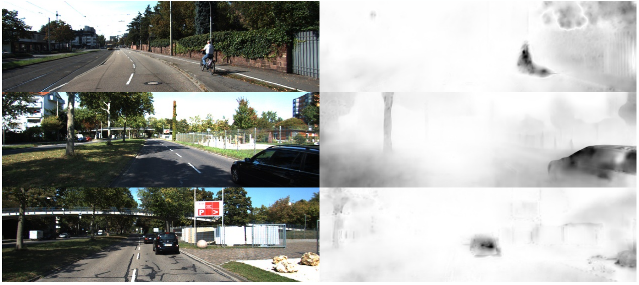
The uncertainty-based depth fusing strategy is utilized to complement challenging artifacts where multi-view geometry fails. As shown in Fig. 4, the moving objects and textureless areas are learned as highly-uncertain regions. Besides, learning the uncertainty in MVS regularizes the cost volume and further improves the depth accuracy on all the metrics (see Tab. 5).

Conclusion

In this paper, we propose MOVEDepth, which crafts monocular cues and velocity guidance for improving multi-frame depth learning in a self-supervised manner. The proposed method leverages monocular depth priority to reduce multi-frame matching geometry ambiguity. Specifically, MOVEDepth constructs cost volume with depth range centered at the monocular priority, and the depth range is adaptively adjusted by the predicted camera velocity. Therefore, video frames with insufficient Triangulation Prior shrink the depth range to monocular priority, and those with sufficient Triangulation Prior expand the depth range to infer more accurate depth. Moreover, we learn depth uncertainty from the entropy of MVS depth probability, which results in a more robust depth against challenging artifacts where multi-view geometry fails. Extensive experiments on KITTI and DDAD show that MOVEDepth achieves stage-of-the-art depth accuracy with significantly reduced depth range. We hope that MOVEDepth can inspire more self-supervised multi-frame depth learning methods in the future.

References

Bae, Budvytis, and Cipolla (2022) Bae, G.; Budvytis, I.; and Cipolla, R. 2022. Multi-View Depth Estimation by Fusing Single-View Depth Probability with Multi-View Geometry. In CVPR.
Casser et al. (2019) Casser, V.; Pirk, S.; Mahjourian, R.; and Angelova, A. 2019. Depth Prediction Without the Sensors: Leveraging Structure for Unsupervised Learning from Monocular Videos. In AAAI.
Chen et al. (2016) Chen, W.; Fu, Z.; Yang, D.; and Deng, J. 2016. Single-Image Depth Perception in the Wild. In NeurIPS.
Chen et al. (2019) Chen, Y.; Schmid, C.; Sminchisescu; and Cristian. 2019. Self-supervised learning with geometric constraints in monocular video: Connecting flow, depth, and camera. In ICCV.
Cheng et al. (2020) Cheng, S.; Xu, Z.; Zhu, S.; Li, Z.; Li, L. E.; Ramamoorthi, R.; and Su, H. 2020. Deep Stereo Using Adaptive Thin Volume Representation With Uncertainty Awareness. In CVPR.
Collins (1996) Collins, R. T. 1996. A space-sweep approach to true multi-image matching. In CVPR.
Dai et al. (2017) Dai, J.; Qi, H.; Xiong, Y.; Li, Y.; Zhang, G.; Hu, H.; and Wei, Y. 2017. Deformable Convolutional Networks. In ICCV.
Deng et al. (2009) Deng, J.; Dong, W.; Socher, R.; Li, L.-J.; Li, K.; and Fei-Fei, L. 2009. Imagenet: A large-scale hierarchical image database. In CVPR.
Ding et al. (2021) Ding, Y.; Yuan, W.; Zhu, Q.; Zhang, H.; Liu, X.; Wang, Y.; and Liu, X. 2021. TransMVSNet: Global Context-aware Multi-view Stereo Network with Transformers. In CVPR.
Eigen and Fergus (2014) Eigen, D.; and Fergus, R. 2014. Predicting Depth, Surface Normals and Semantic Labels with a Common Multi-Scale Convolutional Architecture. In ICCV.
Eigen, Puhrsch, and Fergus (2014) Eigen, D.; Puhrsch, C.; and Fergus, R. 2014. Depth Map Prediction from a Single Image using a Multi-Scale Deep Network. In NeurIPS.
Feng et al. (2022) Feng, Z.; Yang, L.; Jing, L.; Wang, H.; Tian, Y.; and Li, B. 2022. Disentangling Object Motion and Occlusion for Unsupervised Multi-frame Monocular Depth. In ECCV.
Fu et al. (2018) Fu, H.; Gong, M.; Wang, C.; Batmanghelich, K.; and Tao, D. 2018. Deep Ordinal Regression Network for Monocular Depth Estimation. In CVPR.
Galliani, Lasinger, and Schindler (2015) Galliani, S.; Lasinger, K.; and Schindler, K. 2015. Massively Parallel Multiview Stereopsis by Surface Normal Diffusion. In ICCV.
Garg et al. (2016) Garg, R.; Kumar, B. G. V.; Carneiro, G.; and Reid, I. 2016. Unsupervised CNN for Single View Depth Estimation: Geometry to the Rescue. In ECCV.
Geiger, Lenz, and Urtasun (2012) Geiger, A.; Lenz, P.; and Urtasun, R. 2012. Are we ready for autonomous driving? The KITTI vision benchmark suite. In CVPR.
Godard, Aodha, and Brostow (2016) Godard, C.; Aodha, O. M.; and Brostow, G. J. 2016. Unsupervised Monocular Depth Estimation with Left-Right Consistency. In CVPR.
Godard et al. (2018) Godard, C.; Aodha, O. M.; Firman, M.; and Brostow, G. J. 2018. Digging Into Self-Supervised Monocular Depth Estimation. In ICCV.
Gordon et al. (2019) Gordon, A.; Li, H.; Jonschkowski, R.; and Angelova, A. 2019. Depth from videos in the wild: Unsupervised monocular depth learning from unknown cameras. In ICCV.
Gu et al. (2020) Gu, X.; Fan, Z.; Zhu, S.; Dai, Z.; Tan, F.; and Tan, P. 2020. Cascade Cost Volume for High-Resolution Multi-View Stereo and Stereo Matching. In CVPR.
Guizilini et al. (2022) Guizilini, V.; Ambrus, R.; Chen, D.; Zakharov, S.; and Gaidon, A. 2022. Multi-Frame Self-Supervised Depth with Transformers. arXiv, abs/2204.07616.
Guizilini et al. (2019) Guizilini, V.; Ambrus, R.; Pillai, S.; Raventos, A.; and Gaidon, A. 2019. 3D Packing for Self-Supervised Monocular Depth Estimation. In CVPR.
Guizilini et al. (2020) Guizilini, V.; Hou, R.; Li, J.; Ambrus, R.; and Gaidon, A. 2020. Semantically-Guided Representation Learning for Self-Supervised Monocular Depth. In ICLR.
Guizilini et al. (2021) Guizilini, V.; Li, J.; Ambrus, R.; and Gaidon, A. 2021. Geometric Unsupervised Domain Adaptation for Semantic Segmentation. In ICCV.
Ha et al. (2016) Ha, H.; Im, S.; Park, J.; Jeon, H.-G.; and Kweon, I. S. 2016. High-Quality Depth from Uncalibrated Small Motion Clip. In CVPR.
He et al. (2017) He, K.; Gkioxari, G.; Dollár, P.; and Girshick, R. B. 2017. Mask R-CNN. In ICCV.
He et al. (2015) He, K.; Zhang, X.; Ren, S.; and Sun, J. 2015. Deep Residual Learning for Image Recognition. In CVPR.
Hui (2022) Hui, T.-W. 2022. RM-Depth: Unsupervised Learning of Recurrent Monocular Depth in Dynamic Scenes. In CVPR.
Johnston and Carneiro (2020) Johnston, A.; and Carneiro, G. 2020. Self-supervised Monocular Trained Depth Estimation using Self-attention and Discrete Disparity Volume. In CVPR.
Kingma and Ba (2015) Kingma, D. P.; and Ba, J. 2015. Adam: A Method for Stochastic Optimization. In ICLR.
Knapitsch et al. (2017) Knapitsch, A.; Park, J.; Zhou, Q.; and Koltun, V. 2017. Tanks and temples: benchmarking large-scale scene reconstruction. ToG.
Kumar, Bhandarkar, and Prasad (2018) Kumar, A. C.; Bhandarkar, S. M.; and Prasad, M. 2018. DepthNet: A Recurrent Neural Network Architecture for Monocular Depth Prediction. In CVPR.
Kuznietsov et al. (2021) Kuznietsov; Yevhen; Proesmans; Marc; and Van Gool, L. 2021. CoMoDA: Continuous Monocular Depth Adaptation Using Past Experiences. In WACV.
Li et al. (2020) Li, H.; Gordon, A.; Zhao, H.; Casser, V.; and Angelova, A. 2020. Unsupervised monocular depth learning in dynamic scenes. In CoRL.
Lin et al. (2017) Lin, T.; Dollár, P.; Girshick, R. B.; He, K.; Hariharan, B.; and Belongie, S. J. 2017. Feature Pyramid Networks for Object Detection. In CVPR.
Luo et al. (2019) Luo, C.; Yang, Z.; Wang, P.; Wang, Y.; Xu, W.; Nevatia, R.; and Yuille, A. 2019. Every pixel counts++: Joint learning of geometry and motion with 3D holistic understanding. PAMI.
Luo et al. (2020) Luo, X.; Huang, J.-B.; Szeliski, R.; Matzen, K.; and Kopf, J. 2020. Consistent video depth estimation. In SIGGRAPH.
Menze and Geiger (2015) Menze, M.; and Geiger, A. 2015. Object scene flow for autonomous vehicles. In CVPR.
Patil et al. (2020) Patil, V.; Van Gansbeke, W.; Dai, D.; and Van Gool, L. 2020. Don’t Forget The Past: Recurrent Depth Estimation from Monocular Video. In RA-L.
Ranjan et al. (2019) Ranjan, A.; Jampani, V.; Kim, K.; Sun, D.; Wulff, J.; and Black, M. J. 2019. Competitive Collaboration: Joint Unsupervised Learning of Depth, Camera Motion, Optical Flow and Motion Segmentation. In CVPR.
Ronneberger, Fischer, and Brox (2015) Ronneberger, O.; Fischer, P.; and Brox, T. 2015. U-Net: Convolutional Networks for Biomedical Image Segmentation. In MICCAI.
Ruhkamp et al. (2021) Ruhkamp, P.; Gao, D.; Chen, H.; Navab, N.; and Busam, B. 2021. Attention meets Geometry: Geometry Guided Spatial-Temporal Attention for Consistent Self-Supervised Monocular Depth Estimation. In 3DV.
Schonberger et al. (2016) Schonberger, J. L.; Zheng, E.; Frahm, J.-M.; and Pollefeys, M. 2016. Pixelwise View Selection for Unstructured Multi-View Stereo. In ECCV.
Schöps et al. (2017) Schöps, T.; Schönberger, J. L.; Galliani, S.; Sattler, T.; Schindler, K.; Pollefeys, M.; and Geiger, A. 2017. A Multi-view Stereo Benchmark with High-Resolution Images and Multi-camera Videos. In CVPR.
Shao et al. (2022) Shao, S.; Pei, Z.; Chen, W.; Wu, X.; Liu, Z.; and Li, Z. 2022. SMUDLP: Self-Teaching Multi-Frame Unsupervised Endoscopic Depth Estimation with Learnable Patchmatch. arXiv preprint arXiv:2205.15034.
Teed and Deng (2020) Teed, Z.; and Deng, J. 2020. RAFT: Recurrent All-Pairs Field Transforms for Optical Flow. In ECCV.
Wang et al. (2022a) Wang, F.; Galliani, S.; Vogel, C.; and Pollefeys, M. 2022a. IterMVS: Iterative Probability Estimation for Efficient Multi-View Stereo. In CVPR.
Wang et al. (2021) Wang, F.; Galliani, S.; Vogel, C.; Speciale, P.; and Pollefeys, M. 2021. PatchmatchNet: Learned Multi-View Patchmatch Stereo. In CVPR.
Wang, Pizer, and Frahm (2019) Wang, R.; Pizer, S. M.; and Frahm, J.-M. 2019. Recurrent Neural Network for (Un-)Supervised Learning of Monocular Video Visual Odometry and Depth. In CVPR.
Wang, Pang, and Lin (2022) Wang, T.; Pang, J.; and Lin, D. 2022. Monocular 3D Object Detection with Depth from Motion. In ECCV.
Wang et al. (2022b) Wang, X.; Zhu, Z.; Qin, F.; Ye, Y.; Huang, G.; Chi, X.; He, Y.; and Wang, X. 2022b. MVSTER: Epipolar Transformer for Efficient Multi-View Stereo. In ECCV.
Watson et al. (2021) Watson, J.; Aodha, O. M.; Prisacariu, V. A.; Brostow, G. J.; and Firman, M. 2021. The Temporal Opportunist: Self-Supervised Multi-Frame Monocular Depth. In CVPR.
Wimbauer et al. (2020) Wimbauer, F.; Yang, N.; von Stumberg, L.; Zeller, N.; and Cremers, D. 2020. MonoRec: Semi-Supervised Dense Reconstruction in Dynamic Environments from a Single Moving Camera. In CVPR.
Xie, Girshick, and Farhadi (2016) Xie, J.; Girshick, R.; and Farhadi, A. 2016. Deep3D: Fully Automatic 2D-to-3D Video Conversion with Deep Convolutional Neural Networks. In ECCV.
Xu and Tao (2019) Xu, Q.; and Tao, W. 2019. Learning Inverse Depth Regression for Multi-View Stereo with Correlation Cost Volume. In AAAI.
Yang et al. (2018) Yang, N.; Wang, R.; Stückler, J.; and Cremers, D. 2018. Deep Virtual Stereo Odometry: Leveraging Deep Depth Prediction for Monocular Direct Sparse Odometry. In ECCV.
Yao et al. (2018) Yao, Y.; Luo, Z.; Li, S.; Fang, T.; and Quan, L. 2018. MVSNet: Depth Inference for Unstructured Multi-view Stereo. In ECCV.
Yao et al. (2019) Yao, Y.; Luo, Z.; Li, S.; Shen, T.; Fang, T.; and Quan, L. 2019. Recurrent MVSNet for High-Resolution Multi-View Stereo Depth Inference. In CVPR.
Yin et al. (2017) Yin, X.; Wang, X.; Du, X.; and Chen, Q. 2017. Scale Recovery for Monocular Visual Odometry Using Depth Estimated with Deep Convolutional Neural Fields. In ICCV.
Zhang et al. (2019) Zhang, H.; Shen, C.; Li, Y.; Cao, Y.; Liu, Y.; and Yan, Y. 2019. Exploiting temporal consistency for real-time video depth estimation. In ICCV.
Zhang et al. (2020) Zhang, J.; Yao, Y.; Li, S.; Luo, Z.; and Fang, T. 2020. Visibility-aware Multi-view Stereo Network. In BMVC.
Zhou et al. (2017) Zhou, T.; Brown, M.; Snavely, N.; and Lowe, D. G. 2017. Unsupervised Learning of Depth and Ego-Motion from Video. In CVPR.
Zhou et al. (2021) Zhou, Z.; Fan, X.; Shi, P.; and Xin, Y. 2021. R-MSFM: Recurrent Multi-Scale Feature Modulation for Monocular Depth Estimating. In ICCV.

Triangulation Prior Analysis

Binocular systems rely on matching geometry to predict depth $D$ :

D=f\frac{b}{d},

(13)

where $f$ is the focal length, $d$ is the disparity of the matching pixels, and $b$ is the stereo baseline. To make a reliable depth estimation, sufficient Triangulation Prior (Schonberger et al. 2016) is desired. Arguably, Triangulation Prior is represented by baseline $b$ in the stereo systems. In the following, we formulate the stereo baseline in a more general multi-frame setting.

Figure 5: Multi-view geometry in video frames with ego-motion.

As shown in Fig 5, the moving camera captures images at frame $t-1$ and frame $t$ , and the (camera-centered) coordinates of the observed object are $(X_{1},Y_{1},D_{1})^{\text{T}}$ and $(X_{2},Y_{2},D_{2})^{\text{T}}$ . Given camera extrinsic $\mathbf{R}$ and $\mathbf{T}$ , the transformation brought by ego-motion is formulated as:

\left(\begin{array}[]{c}X_{2}\\ Y_{2}\\ D_{2}\end{array}\right)=\mathbf{R}\left(\begin{array}[]{c}X_{1}\\ Y_{1}\\ D_{1}\end{array}\right)+\mathbf{T}.

(14)

Given camera intrinsic:

\mathbf{K}=\left(\begin{array}[]{ccc}f&0&c_{u}\\ 0&f&c_{v}\\ 0&0&1\end{array}\right),

(15)

we can calculate the corresponding pixel locations of $(X_{1},Y_{1},D_{1})^{\text{T}}$ and $(X_{2},Y_{2},D_{2})^{\text{T}}$ :

\left(\begin{array}[]{c}u_{2}\\ v_{2}\\ 1\end{array}\right)=\frac{1}{D_{2}}\left(\begin{array}[]{lll}f&0&c_{u}\\ 0&f&c_{v}\\ 0&0&1\end{array}\right)\left(\begin{array}[]{l}X_{2}\\ Y_{2}\\ D_{2}\end{array}\right),

(16)

\left(\begin{array}[]{c}u_{1}\\ v_{1}\\ 1\end{array}\right)=\frac{1}{D_{1}}\left(\begin{array}[]{lll}f&0&c_{u}\\ 0&f&c_{v}\\ 0&0&1\end{array}\right)\left(\begin{array}[]{l}X_{1}\\ Y_{1}\\ D_{1}\end{array}\right).

(17)

Constrained by Eq. 14, Eq. 16, and Eq. 17, the depth at frame $t$ can be derived as:

D_{2}=f\frac{\mathbf{R_{3}}\left(\begin{array}[]{c}\frac{u_{1}-c_{u}}{f}\\ \frac{v_{1}-c_{v}}{f}\\ 1\end{array}\right)T_{1}-\mathbf{R_{1}}\left(\begin{array}[]{c}\frac{u_{1}-c_{u}}{f}\\ \frac{v_{1}-c_{v}}{f}\\ 1\end{array}\right)T_{3}}{\mathbf{R_{3}}\left(\begin{array}[]{c}\frac{u_{1}-c_{u}}{f}\\ \frac{v_{1}-c_{v}}{f}\\ 1\end{array}\right)\left(u_{2}-c_{u}\right)-\mathbf{R_{1}}\left(\begin{array}[]{c}\frac{u_{1}-c_{u}}{f}\\ \frac{v_{1}-c_{v}}{f}\\ 1\end{array}\right)f},

(18)

where $\mathbf{R_{1}}$ , $\mathbf{R_{3}}$ are the 1-st and 3-rd row vector of $\mathbf{R}$ , and $T_{1},T_{3}$ are the 1-st and 3-rd scalar of $\mathbf{T}$ .

Considering cameras in the driving scenario where the car has no ego-rotation, we can set $\mathbf{R}$ to the identity matrix. Then the depth is simplified as follows:

D_{2}=\frac{f(T_{1}-\frac{u_{1}-c_{u}}{f}T_{3})}{u_{2}-u_{1}}.

(19)

Arguably, the camera moves at a constant speed during the frame interval. Therefore, $T_{1},T_{3}$ can be formulated by camera velocity:

T_{1}=\alpha V_{x},\quad T_{3}=\alpha V_{z},

(20)

where $\alpha$ is the camera frame rate. As shown in Fig 6, $V_{x}$ and $V_{z}$ is the camera speed along the x-axis and z-axis, and they satisfy:

V_{x}=V_{z}\tan\gamma,

(21)

where $\gamma$ is the yaw angle of the moving camera and $\gamma\approx 0$ in the driving scenario. Finally, the depth at frame $t$ is:

D_{2}=f\frac{\alpha(\tan\gamma-\frac{u_{1}-c_{u}}{f})V_{z}}{u_{2}-u_{1}}.

(22)

Compared with the binocular system (Eq. 13), we can formulate the general disparity and baseline in the multi-frame system: $u_{2}-u_{1}$ is the general disparity, and $\alpha(\tan\gamma-\frac{u_{1}-c_{u}}{f})V_{z}$ is the general baseline, where the per-pixel baseline is positively related to the camera velocity.

Therefore, it is concluded that a higher camera velocity brings a larger baseline, which provides sufficient Triangulation Prior for the multi-frame system. In contrast, slow camera motion provides a little baseline, and the Triangulation Prior is limited.

Figure 6: Illustration of the camera moving at a constant speed.

Additional Implementation Details

Recent learning-based Multi-View Stereo (MVS) methods adopt Deformable Convolutional Networks (DCNs) (Dai et al. 2017) or Transformer blocks (Ding et al. 2021; Guizilini et al. 2022) to enhance the feature learning. However, in this paper, the feature extractor $\theta_{\text{enc}}$ and cost volume decoder $\theta_{\text{dec}}$ only comprise of 2D/3D Convolutional Neural Networks (CNNs), because the argument of our paper is to verify the effectiveness of Monocular Depth Priority and Velocity-Guided sampling.

Network Architecture of Feature Extractor

We use a four-stage Feature Pyramid Network (FPN) (Lin et al. 2017) to extract multi-frame features, and the detailed parameters with layer descriptions are summarized in Table 6. Notably, we only leverage features from Stage 3 as the output, whose resolution is $\frac{1}{4}$ of the original image.

Table 6: The detailed parameters of

\theta_{\text{enc}}

, where S denotes stride, and if not specified with *, each convolution layer is followed by a Batch Normalization layer (BN) and a Rectified Linear Unit (ReLU).

Stage Description	Layer Description	Output Size
-	Input Images	$H\times W\times 3$
FPN Stage 1	Conv2D, $3\times 3$ , S1, 8	$H\times W\times 8$
FPN Stage 1	Conv2D, $3\times 3$ , S1, 8	$H\times W\times 8$
FPN Stage 2	Conv2D, $5\times 5$ , S2, 16	$H/2\times W/2\times 16$
FPN Stage 2	Conv2D, $3\times 3$ , S1, 16	$H/2\times W/2\times 16$
FPN Stage 2	Conv2D, $3\times 3$ , S1, 16	$H/2\times W/2\times 16$
FPN Stage 3	Conv2D, $5\times 5$ , S2, 32	$H/4\times W/4\times 32$
FPN Stage 3	Conv2D, $3\times 3$ , S1, 32	$H/4\times W/4\times 32$
FPN Stage 3	Conv2D, $3\times 3$ , S1, 32	$H/4\times W/4\times 32$
FPN Stage 3 Inner Layer*	Conv2D, $1\times 1$ , S1, 64	$H/4\times W/4\times 64$
FPN Stage 3 Output Layer*	Conv2D, $1\times 1$ , S1, 32	$H/4\times W/4\times 32$
FPN Stage 4	Conv2D, $5\times 5$ , S2, 64	$H/8\times W/8\times 64$
FPN Stage 4	Conv2D, $3\times 3$ , S1, 64	$H/8\times W/8\times 64$
FPN Stage 4	Conv2D, $3\times 3$ , S1, 64	$H/8\times W/8\times 64$
FPN Stage 4 Inner Layer*	Conv2D, $1\times 1$ , S1, 64	$H/8\times W/8\times 64$

Network Architecture of Cost Volume Decoder

An UNet (Ronneberger, Fischer, and Brox 2015) structured 3D CNN is adopted for decoding MVS cost volume, and the network details are in Table 7.

Table 7: The detailed parameters of

\theta_{\text{dec}}

, where S denotes stride, and if not specified with *, each convolution layer is followed by a Batch Normalization layer (BN) and a Rectified Linear Unit (ReLU).

Stage Description	Layer Description	Output Size
-	Input Cost Volume	$H/4\times W/4\times 16\times 16$
UNet Stage 1	Conv3D, $3\times 3\times 3$ , S1, 16	$H/4\times W/4\times 16\times 16$
UNet Stage 1	Conv3D, $3\times 3\times 3$ , S2, 32	$H/8\times W/8\times 16\times 32$
UNet Stage 1	Conv3D, $3\times 3\times 3$ , S1, 32	$H/8\times W/8\times 16\times 32$
UNet Stage 1 Inner Layer	TransposeConv3D, $3\times 3\times 3$ , S2, 16	$H/2\times W/2\times 16\times 16$
UNet Stage 1 Output Layer*	TransposeConv3D, $3\times 3\times 3$ , S1, 16	$H/2\times W/2\times 16\times 16$
UNet Stage 2	Conv3D, $3\times 3\times 3$ , S2, 64	$H/16\times W/16\times 16\times 64$
UNet Stage 2	Conv3D, $3\times 3\times 3$ , S1, 64	$H/16\times W/16\times 16\times 64$
UNet Stage 2 Inner Layer	TransposeConv3D, $3\times 3\times 3$ , S2, 32	$H/8\times W/8\times 16\times 32$
UNet Stage 3	Conv3D, $3\times 3\times 3$ , S2, 128	$H/32\times W/32\times 16\times 128$
UNet Stage 3	Conv3D, $3\times 3\times 3$ , S1, 128	$H/32\times W/32\times 16\times 128$
UNet Stage 3 Inner Layer	TransposeConv3D, $3\times 3\times 3$ , S2, 64	$H/16\times W/16\times 16\times 64$

Evaluation Metrics

Following previous depth estimation methods (Godard et al. 2018; Watson et al. 2021; Feng et al. 2022), we use Absolute Relative Error (Abs. Rel.), Squared Relative Error (Sq. Rel.), Root Mean Squared Error (RMSE), Root Mean Squared Log Error ( $\text{RMSE}_{\text{log}}$ ), and $\delta_{1},\delta_{2},\delta_{3}$ as the metrics to evaluate the depth prediction performance. These metrics are formulated as:

	$\displaystyle\mathrm{Abs.Rel.}$	$\displaystyle=\frac{1}{n}\sum_{i}\frac{\|p_{i}-g_{i}\|}{g_{i}}$
	$\displaystyle\mathrm{Sq.Rel.}$	$\displaystyle=\frac{1}{n}\sum_{i}\frac{(p_{i}-g_{i})^{2}}{g_{i}}$
	$\displaystyle\mathrm{RMSE}$	$\displaystyle=\sqrt{\frac{1}{n}\sum_{i}(p_{i}-g_{i})^{2}}$
	$\displaystyle\mathrm{RMSE_{log}}$	$\displaystyle=\sqrt{\frac{1}{n}\sum_{i}(\log p_{i}-\log g_{i})^{2}},$

and $\delta_{1},\delta_{2},\delta_{3}=\%\ of\ thresh<1.25,1.25^{2},1.25^{3},$ where $g$ and $p$ are the depth values of ground truth and prediction in meters, $thresh=\max(\frac{g}{p},\frac{p}{g})$ .

Crafting Monocular Cues and Velocity Guidance for Self-Supervised Multi-Frame Depth Learning

Abstract

Introduction

Related Work

Monocular Depth Learning

Multi-Frame Depth Learning

Method

Self-Supervised Monocular Depth Learning

MOVEDepth Design

MVS Depth from Monocular Depth Priority

Velocity-Guided Depth Sampling

Uncertainty-Based Depth Fusing

Loss Function

Experiment

Datasets

Implementation Details

KITTI Results

DDAD Results

Ablation Study

Monocular Priority for Multi-Frame Depth Learning

Velocity-Guided Depth Sampling

Uncertainty-Based Depth Fusing

Conclusion

References

Triangulation Prior Analysis

Additional Implementation Details

Network Architecture of Feature Extractor

Network Architecture of Cost Volume Decoder

Evaluation Metrics

Crafting Monocular Cues and Velocity Guidance for
Self-Supervised Multi-Frame Depth Learning