Gluonic evanescent operators: two-loop anomalous dimensionsPreprint: USTC-ICTS/PCFT-22-23

The Lagrangian of the pure YM theory is²² 2 For simplicity, in this paper we will not distinguish upper and lower Lorentz indices. For example, $\eta^{\mu\nu}$ and $\delta^{\mu}_{\nu}$ are regarded as equivalent. This will not cause any problem in the flat spacetime.

$\displaystyle\mathcal{L}=-\frac{1}{2}\text{tr}(F_{\mu\nu}F_{\mu\nu})=-\frac{1}{4}F^{a}_{\mu\nu}F^{a}_{\mu\nu}\,,$

(1)

where $F_{\mu\nu}\equiv F^{a}_{\mu\nu}T^{a}$, and $T^{a},\ \text{with }a=1,..,N_{c}^{2}-1$, is the SU($N_{c}$) generator. The field strength tensor $F^{a}_{\mu\nu}$ is defined as

$\displaystyle F^{a}_{\mu\nu}=\partial_{\mu}A_{\nu}^{a}-\partial_{\nu}A_{\mu}^{a}+g_{0}f^{abc}A_{\mu}^{b}A_{\nu}^{c}\,,$

(2)

where $A_{\mu}^{a}$ is the gauge field, $f^{abc}$ is the structure constant and $g_{0}$ is the bare coupling. The Einstein summation is assumed for the repeated indices.

The covariant derivative is defined to be

$\displaystyle D_{\mu}=\partial_{\mu}-\text{i}g_{0}A_{\mu}^{a}T^{a}\,.$

(3)

The action of the covariant derivative is

$\displaystyle D_{\mu}X\equiv[D_{\mu},X]\,,$

(4)

given that $X=X^{a}T^{a}$. The commutator of two $D_{\mu}$’s reads

$\displaystyle[D_{\mu},D_{\nu}]=-\text{i}g_{0}F_{\mu\nu}\,.$

(5)

The equation of motion reads

$\displaystyle D_{\mu}F_{\mu\nu}=0\,.$

(6)

Another important relationship is the Bianchi identity:

$\displaystyle D_{\mu}F_{\rho\sigma}=D_{\sigma}F_{\rho\mu}+D_{\rho}F_{\mu\sigma}\,.$

(7)

We aim to study the gauge-invariant local scalar operators. For simplicity, in this paper we will take the large $N_{c}$ limit. Consequently, we only need to consider the single-trace operators. We will often abbreviate the Lorentz indices by integer numbers, such as

$\displaystyle\text{tr}(F_{12}F_{12})\equiv\text{tr}(F_{\mu_{1}\mu_{2}}F_{\mu_{1}\mu_{2}})\,.$

(8)

It is conventional to classify the operators according to their classical dimensions. For example, we say that $\text{tr}(F_{12}F_{12})$ is a dimension-4 operator.

Given an operator $O$, its $n$-point form factor is defined to be

$\displaystyle\mathcal{F}_{O,\text{$n$ gluons}}=\int\text{d}^{d}xe^{-{\text{i}}q\cdot x}\langle\text{g}_{1}\cdots,\text{g}_{n}|O|0\rangle\,,$

(9)

where $\text{g}_{i}$ denotes an external gluon carrying an on-shell momenta $p_{i}$, and $q=\sum_{i}{p_{i}}$ is the off-shell momentum associated to the operator. See e.g. Yang:2019vag for a recent introduction of form factors. All the gluons are assumed to be outgoing in this paper. For an operator $O$, there exists an integer number $m$ such that its tree-level $n$-point form factors vanish unless $n\geq m$. We call the $m$-gluon form factor the minimal form factor of this operator. Similarly, an $(m+1)$-point form factor is called a next-to-minimal form factor, and a $(m-1)$-point form factor is called a sub-minimal form factor. The tree-level color-ordered minimal form factor can be achieved straightforwardly by the dictionary (see e.g. Jin:2022ivc)

$\displaystyle F^{\mu\nu}\to\text{i}(p^{\mu}e^{\nu}-p^{\nu}e^{\mu}),\qquad D^{\mu}\to\text{i}p^{\mu}\,,$

(10)

where $e^{\mu}$ is the polarization of a gluon and $p^{\mu}$ is the momentum of a gluon. By definition, there is no tree-level sub-minimal form factor. For the tree-level next-to-minimal form factors, compact formulas are given in Jin:2022ivc.

The length of an operator is defined to be the number of gluons of its minimal form factor.³³ 3 In most cases, one can simply take the length as equal to the number of $F_{\mu\nu}$ in an operator. However, this may cause ambiguity sometimes. For example, the operator $\text{tr}([D_{1},D_{2}]F_{34}F_{41}F_{23})=-ig_{0}\text{tr}([F_{12},F_{34}]F_{41}F_{23})$ do not have a definite length by counting the number of $F_{\mu\nu}$; while using the above definition based on the minimal form factor, this operator is of length 4. For example, the operator

$\displaystyle\text{tr}(D_{3}D_{4}F_{12}F_{23}F_{41})+D^{4}\big(\text{tr}(F_{12}F_{12})\big)\,,$

(11)

contains a length-3 and a length-2 monomial operators. The length of the whole operator is two, since the minimal tree form factor is a two-point form factor. In this work, we take the convention such that each length-$L$ monomial operator is implicitly multiplied by a factor $(-\text{i}g_{0})^{L-2}$. For example, (11) means $(-\text{i}g_{0})\text{tr}(D_{3}D_{4}F_{12}F_{23}F_{41})+D^{4}\big(\text{tr}(F_{12}F_{12})\big)$. This convention is due to the fact that a strength tensor can be interpreted as a commutator of two $D_{\mu}$’s which involves a factor $-\text{i}g_{0}$, and the shortest operator in this work is of length two. Under charge conjugation, the color trace of a monomial operator is reversed, together with a factor $(-1)^{L}$ with $L$ the length of the monomial operator Bardeen:1969md. For example,

$\displaystyle{\rm tr}(D_{3}D_{4}F_{12}F_{23}F_{41})\to-{\rm tr}(F_{41}F_{23}D_{3}D_{4}F_{12})\,.$

(12)

An eigenstate operator under change conjugation with $+\ (-)$ C-parity is said to be C-even (C-odd).

An operator before renormalization is called a bare operator, denoted as $O_{\text{b}}$. Since we aim to study the evanescent operators, we will adopt the CDR scheme to regularize the divergences of a bare operator, with loop momenta and external momenta all in $d$ spacetime dimensions. Given a set of bare operators $\{O_{\text{b},j}\}$, a renormalized operator $O_{i}$ can be written as

$\displaystyle{O}_{i}=Z_{i}^{~j}{O}_{\text{b},j}\,.$

(13)

A matrix element $Z^{~j}_{i}$ represents an operator mixing from $O_{i,\text{b}}$ to $O_{j,\text{b}}$. In general, operators of the same classical dimension can mix with each other. The dilatation matrix $\mathcal{D}$ is defined as

$\displaystyle\mathcal{D}\equiv-\mu\frac{\text{d}Z}{\text{d}\mu}Z^{-1}=\sum_{l=1}\left(\frac{\alpha_{s}}{4\pi}\right)^{l}\mathcal{D}^{(l)}\,.$

(14)

The eigenvalues of the dilatation matrix are the anomalous dimensions, denoted as $\gamma$.

We call an operator a physical operator if it does not vanish in four spacetime dimensions. Otherwise, we call it an evanescent operator. For example, the operator

$\displaystyle\delta^{12345}_{6789(10)}\text{tr}(F_{12}F_{34}F_{56}F_{78}F_{9(10)})\,,$

(15)

is an evanescent operator, where the generalized Kronecker symbol is defined to be

$$\delta^{\mu_{1}..\mu_{n}}_{\nu_{1}...\nu_{n}}={\rm det}(\delta^{\mu}_{\nu})=\left|\begin{matrix}\delta^{\mu_{1}}_{\nu_{1}}&\ldots&\delta^{\mu_{1}}_{\nu_{n}}\\ \vdots&&\vdots\\ \delta^{\mu_{n}}_{\nu_{1}}&\ldots&\delta^{\mu_{n}}_{\nu_{n}}\end{matrix}\right|\,.$$

(16)

One can see that the rank-5 Kronecker symbol guarantees the vanishing of (15) in four spacetime dimensions. More details of systematic construction of evanescent operators can be found in Jin:2022ivc.

We will choose the dimension-10 operators as concrete examples to study the effects of evanescent operators on the two-loop renormalization. As mentioned above, we will consider the large $N_{c}$ limit and thus we focus only on the single-trace operators. The arrangement of our operator basis is summarized in Table 1. The basis is first divided into two classes: the physical ones and the evanescent ones. Within each class, we classify the operators according to their C-parities and then into different lengths. The physical operators can be further arranged into different helicity sectors—within each helicity sector, the operators’ tree minimal form factors are only non-vanishing in the corresponding helicity configuration (and the conjugate configuration). For example, $\text{tr}(F_{12}F_{12})$ is in the $(-)^{2}$ sector and its tree-level minimal form factor is non-vanishing only if the helicities are $(-)^{2}$ or $(+)^{2}$. The explicit definitions of the operators are given in Appendix A. A similar basis has been given in Jin:2022ivc. Here an improvement is made: the basis is reorganized in a form such that the total derivative operators are separated explicitly, see Appendix A for further details. This reorganization will help to analyze the comparison of the anomalous dimensions in different renormalization schemes in Section 5.1.

Before showing how to calculate the $Z$ matrix, in this section we first give a description of the blockwise structure of the $Z$ matrix resulting from our operator basis choice in Section 2.2. The operators are divided into physical and evanescent operators, and we recall that physical operators refer to those that are non-vanishing in four spacetime dimensions. The $Z$ matrix has the following structure

$\displaystyle\left(\begin{array}[]{cc}Z_{\text{pp}}&Z_{\text{pe}}\\ Z_{\text{ep}}&Z_{\text{ee}}\end{array}\right).$

In a subscript, an “e” denotes “evanescent” and a “p” denotes “physical”. For example, the $Z_{\text{pp}}$ denotes the block of physical-to-physical mixing. Other blocks are similarly defined. Since there is no mixing between the C-even and C-odd operators, the $Z$ matrix can be further divided into

$\displaystyle\left(\begin{array}[]{cccc}Z_{\text{pp}}^{\text{even}}&0&Z_{\text{pe}}^{\text{even}}&0\\ 0&Z_{\text{pp}}^{\text{odd}}&0&Z_{\text{pe}}^{\text{odd}}\\ Z_{\text{ep}}^{\text{even}}&0&Z_{\text{ee}}^{\text{even}}&0\\ 0&Z_{\text{ep}}^{\text{odd}}&0&Z_{\text{ee}}^{\text{odd}}\\ \end{array}\right)\,.$

Each block can be further arranged according to the lengths of the operators as follows

		$\displaystyle Z_{\text{pp}}^{\text{even}}=\left(\begin{array}[]{cccc}Z_{\text{pp},2\to 2}^{\text{even}}&Z_{\text{pp},2\to 3}^{\text{even}}&Z_{\text{pp},2\to 4}^{\text{even}}&Z_{\text{pp},2\to 5}^{\text{even}}\\ Z_{\text{pp},3\to 2}^{\text{even}}&Z_{\text{pp},3\to 3}^{\text{even}}&Z_{\text{pp},3\to 4}^{\text{even}}&Z_{\text{pp},3\to 5}^{\text{even}}\\ Z_{\text{pp},4\to 2}^{\text{even}}&Z_{\text{pp},4\to 3}^{\text{even}}&Z_{\text{pp},4\to 4}^{\text{even}}&Z_{\text{pp},4\to 5}^{\text{even}}\\ Z_{\text{pp},5\to 2}^{\text{even}}&Z_{\text{pp},5\to 3}^{\text{even}}&Z_{\text{pp},5\to 4}^{\text{even}}&Z_{\text{pp},5\to 5}^{\text{even}}\\ \end{array}\right)\,,$		$\displaystyle Z_{\text{pp}}^{\text{odd}}=\left(\begin{array}[]{cc}Z_{\text{pp},3\to 3}^{\text{odd}}&Z_{\text{pp},3\to 4}^{\text{odd}}\\ Z_{\text{pp},4\to 3}^{\text{odd}}&Z_{\text{pp},4\to 4}^{\text{odd}}\\ \end{array}\right)\,,$
		$\displaystyle Z_{\text{pe}}^{\text{even}}=\left(\begin{array}[]{cc}Z_{\text{pe},2\to 4}^{\text{even}}&Z_{\text{pe},2\to 5}^{\text{even}}\\ Z_{\text{pe},3\to 4}^{\text{even}}&Z_{\text{pe},3\to 5}^{\text{even}}\\ Z_{\text{pe},4\to 4}^{\text{even}}&Z_{\text{pe},4\to 5}^{\text{even}}\\ Z_{\text{pe},5\to 4}^{\text{even}}&Z_{\text{pe},5\to 5}^{\text{even}}\\ \end{array}\right)\,,$		$\displaystyle Z_{\text{pe}}^{\text{odd}}=\left(\begin{array}[]{c}Z_{\text{pe},3\to 4}^{\text{odd}}\\ Z_{\text{pe},4\to 4}^{\text{odd}}\\ \end{array}\right)\,,$
		$\displaystyle Z_{\text{ep}}^{\text{even}}=\left(\begin{array}[]{cccc}Z_{\text{ep},4\to 2}^{\text{even}}&Z_{\text{ep},4\to 3}^{\text{even}}&Z_{\text{ep},4\to 4}^{\text{even}}&Z_{\text{ep},4\to 5}^{\text{even}}\\ Z_{\text{ep},5\to 2}^{\text{even}}&Z_{\text{ep},5\to 3}^{\text{even}}&Z_{\text{ep},5\to 4}^{\text{even}}&Z_{\text{ep},5\to 5}^{\text{even}}\\ \end{array}\right)\,,$		$\displaystyle Z_{\text{ep}}^{\text{odd}}=\left(\begin{array}[]{cc}Z_{\text{ep},4\to 3}^{\text{odd}}&Z_{\text{ep},4\to 4}^{\text{odd}}\\ \end{array}\right)\,,$
		$\displaystyle Z_{\text{ee}}^{\text{even}}=\left(\begin{array}[]{cc}Z_{\text{ee},4\to 4}^{\text{even}}&Z_{\text{ee},4\to 5}^{\text{even}}\\ Z_{\text{ee},5\to 4}^{\text{even}}&Z_{\text{ee},5\to 5}^{\text{even}}\\ \end{array}\right)\,,$		$\displaystyle Z_{\text{ee}}^{\text{odd}}=\left(\begin{array}[]{c}Z_{\text{ee},4\to 4}^{\text{odd}}\\ \end{array}\right)\,,$

where $Z_{L\to L^{\prime}}$ represents the mixing from length-$L$ operators to length-$L^{\prime}$ operators. The dilatation matrix $\mathcal{D}$, defined in (14), has the same structure as the $Z$ matrix.

The anomalous dimensions are the eigenvalues of $\mathcal{D}$, which are given by the equation

$\displaystyle\text{Det}\left(\mathcal{D}-\boldsymbol{1}\ \gamma\right)=0\,,$

(41)

where Det$(M)$ means the determinant of the matrix $M$ and $\boldsymbol{1}$ denotes the identity matrix. $\gamma$ can be expanded in the coupling constant as

$\displaystyle\gamma=\sum_{l=1}\left(\frac{\alpha_{s}}{4\pi}\right)^{l}\gamma^{(l)}\,.$

(42)

In this work, we give a calculation of the anomalous dimensions up to two loops. At the one-loop order, an operator would not mix with operators of lower lengths. In other words, $Z^{(1)}$ is a block upper triangular matrix according to the lengths of operators. Based on this fact, it is not hard to derive that the calculation of two-loop anomalous dimensions only requires the blocks $Z^{(1)}_{L\to L}$, $Z^{(1)}_{L\to L+1}$, $Z^{(2)}_{L\to L-1}$ and $Z^{(2)}_{L\to L}$.

Form factors of bare operators (i.e. bare form factors) involve both the ultraviolet (UV) divergences and the the infrared (IR) divergences. The $Z$ matrix is the renormalization matrix to absorb the UV divergences and can be calculated by requiring that renormalized form factors have only IR divergences. Below we give a detailed discussion about the divergences and renormalization of form factors. The computation of bare form factors will be the topic of the next section.

According to (13), the form factor of an renormalized operator $O_{i}$ reads

$\displaystyle\mathcal{F}_{i}=Z_{i}^{\ j}\mathcal{F}_{j,\text{b}}\,,$

(43)

where $\{\mathcal{F}_{j,\text{b}}\}$ are the bare form factors. The $n$-point bare form factors can be expanded as

$\displaystyle\mathcal{F}_{i,\text{b}}=g_{0}^{\delta_{n}}\sum_{l=0}\left(\frac{\alpha_{0}}{4\pi}\right)^{l}\mathcal{F}_{i,\text{b}}^{(l)}\,,$

(44)

with $\alpha_{0}=\frac{g_{0}^{2}}{4\pi}$ the bare coupling constant and $\delta_{n}$ equal $(n-2)$ according to the convention that each monomial operator has a factor $(-\text{i}g_{0})^{L-2}$ as mentioned in Section 2.1. In the $\overline{\text{MS}}$ scheme, the two-loop renormalization of $\alpha_{0}$ reads (see e.g. Gehrmann:2011aa)

$\displaystyle\alpha_{0}=\alpha_{s}S_{\epsilon}^{-1}\mu^{2\epsilon}\left(1-\frac{\beta_{0}}{\epsilon}\frac{\alpha_{s}}{4\pi}+\left(\frac{\beta_{0}^{2}}{\epsilon^{2}}-\frac{\beta_{1}}{2\epsilon}\right)\left(\frac{\alpha_{s}}{4\pi}\right)^{2}+\mathcal{O}(\alpha_{s}^{3})\right)\,,$

(45)

where $\alpha_{s}=\frac{g_{s}^{2}}{4\pi}$ is the renormalized coupling constant, $S_{\epsilon}=(4\pi e^{\gamma_{E}})^{\epsilon}$, and $\mu$ is the renormalization scale. The constants in (45) are

$\displaystyle\beta_{0}=\frac{11N_{c}}{3},\quad\beta_{1}=\frac{34N_{c}^{2}}{3}\,.$

(46)

The $Z$ matrix can be expanded as

$\displaystyle Z^{\ j}_{i}=\delta^{j}_{i}+\sum_{l=1}\left(\frac{\alpha_{s}}{4\pi}\right)^{l}{{Z^{(l)}}^{\ j}_{i}}\,.$

(47)

Substituting (47) into (14), together with the beta function in the pure Yang-Mills theory:

$\displaystyle\mu\frac{\text{d}\alpha_{s}}{\text{d}\mu}=-2\epsilon\alpha_{s}-\frac{\beta_{0}}{2\pi}\alpha_{s}^{2}+\mathcal{O}(\alpha_{s}^{3})\,,$

(48)

one obtains the expansion of the dilatation matrix as

		$\displaystyle\mathcal{D}^{(1)}=2\epsilon Z^{(1)}\,,$		(49)
		$\displaystyle\mathcal{D}^{(2)}=4\epsilon Z^{(2)}-2\epsilon\left(Z^{(1)}\right)^{2}+2\beta_{0}Z^{(1)}\,.$		(50)

According to (50), a finite two-loop dilatation matrix requires the following matrix equation

$\displaystyle Z^{(2)}|_{\frac{1}{\epsilon^{2}}-\text{part}}=\Big(\frac{1}{2}(Z^{(1)})^{2}-\frac{\beta_{0}}{2\epsilon}Z^{(1)}\Big)|_{\frac{1}{\epsilon^{2}}-\text{part}}\,.$

(51)

A renormalized form factor can be expanded in the renormalized coupling $\alpha_{s}$ in a form similar to (44),

$\displaystyle\mathcal{F}_{i}=g_{s}^{\delta_{n}}S_{\epsilon}^{-\frac{\delta_{n}}{2}}\sum_{l=0}\left(\frac{\alpha_{s}}{4\pi}\right)^{l}\mathcal{F}_{i}^{(l)}\,,$

(52)

The relations between ${\cal F}_{i}$ and ${\cal F}_{i,{\rm b}}$ can be obtained using (3.9), (3.11) and (3.13), and up to the two-loop order, they are given by

		$\displaystyle\mathcal{F}_{i}^{(0)}=\mathcal{F}_{i,\text{b}}^{(0)}\,,$		(53)
		$\displaystyle\mathcal{F}_{i}^{(1)}=S_{\epsilon}^{-1}\mathcal{F}_{i,\text{b}}^{(1)}+\left({Z^{(1)}}_{i}^{\ j}-\frac{\delta_{n}}{2}\frac{\beta_{0}}{\epsilon}\delta^{\ j}_{i}\right)\mathcal{F}_{j,\text{b}}^{(0)}\,,$		(54)
		$\displaystyle\mathcal{F}_{i}^{(2)}=S_{\epsilon}^{-2}\mathcal{F}_{i,\text{b}}^{(2)}+S_{\epsilon}^{-1}\left({Z^{(1)}}^{\ j}_{i}-\left(1+\frac{\delta_{n}}{2}\right)\frac{\beta_{0}}{\epsilon}\delta^{\ j}_{i}\right)\mathcal{F}_{j,\text{b}}^{(1)}$
		$\displaystyle\quad\qquad+\left({Z^{(2)}}^{\ j}_{i}-\frac{\delta_{n}}{2}\frac{\beta_{0}}{\epsilon}{Z^{(1)}}^{\ j}_{i}+\frac{\delta_{n}^{2}+2\delta_{n}}{8}\frac{\beta_{0}^{2}}{\epsilon^{2}}\delta^{\ j}_{i}-\frac{\delta_{n}}{4}\frac{\beta_{1}}{\epsilon}\delta^{\ j}_{i}\right)\mathcal{F}_{j,\text{b}}^{(0)}\,,$		(55)

A renormalized form factor only involves the IR divergences. The IR divergences is well understood, and up to two loops, the IR divergences of renormalized form factors take the universal form as Catani:1998bh

		$\displaystyle\mathcal{F}_{i}^{(1)}\big|_{\text{div}}=\mathcal{F}_{i}^{(1)}\big|_{\text{IR}}=I^{(1)}(\epsilon)\mathcal{F}_{i}^{(0)}\,,$		(56)
		$\displaystyle\mathcal{F}_{i}^{(2)}\big|_{\text{div}}=\mathcal{F}_{i}^{(2)}\big|_{\text{IR}}=I^{(2)}(\epsilon)\mathcal{F}_{i}^{(0)}+I^{(1)}(\epsilon)\mathcal{F}_{i}^{(1)}\,,$		(57)

The factors $I^{(1)}$ and $I^{(2)}$ read

	$\displaystyle I_{n}^{(1)}(\epsilon)$	$\displaystyle=-{e^{\gamma_{E}\epsilon}\over\Gamma(1-\epsilon)}\bigg(\frac{N_{c}}{\epsilon^{2}}+\frac{\beta_{0}}{2\epsilon}\bigg)\sum_{i=1}^{n}(-{s_{i,i+1}})^{-\epsilon}\,,$		(58)
	$\displaystyle I_{n}^{(2)}(\epsilon)$	$\displaystyle=-{1\over 2}\big[I^{(1)}(\epsilon)\big]^{2}-{\beta_{0}\over\epsilon}I^{(1)}(\epsilon)+{e^{-\gamma_{E}\epsilon}\Gamma(1-2\epsilon)\over\Gamma(1-\epsilon)}\left[\frac{\beta_{0}}{\epsilon}+{\cal K}\right]I^{(1)}(2\epsilon)+n{e^{\gamma_{E}\epsilon}\over\epsilon\Gamma(1-\epsilon)}{\cal H}_{\Omega,g}^{(2)}\,,$

with

$\displaystyle{\cal K}=\left({67\over 9}-{\pi^{2}\over 3}\right)N_{c}\,,\qquad{\cal H}_{\Omega,g}^{(2)}=\left(\frac{\zeta_{3}}{2}+{5\over 12}+{11\pi^{2}\over 144}\right)N_{c}^{2}\,.$

(59)

By requiring that (54) and (55) have the same divergences as (56) and (57), namely

$$\mathcal{F}_{i}^{(\ell)}-\mathcal{F}_{i}^{(1)}\big|_{\text{IR}}={\cal O}(\epsilon^{0})\,,$$

one can build linear equations between ${Z^{(l)}}$’s and bare form factors. The ${\cal O}(\epsilon^{0})$ term depends on the renormalization scheme. For example, the linear equations for the $\overline{\text{MS}}$ scheme are given in (60) and (61).

The definition of the $Z$ matrix depends on the choice of renormalization schemes. In this subsection, we discuss $Z$ matrix in the $\overline{\text{MS}}$ scheme Bardeen:1978yd and the finite renormalization scheme Buras:1989xd; Bondi:1989nq; Dugan:1990df in Section 3.3.1 and Section 3.3.2 respectively. We will show that it is easier to compute the physical anomalous dimensions in the finite renormalization scheme.

The main strategy of our calculation is based on a combination of the unitarity method Bern:1994cg; Bern:1994zx; Britto:2004nc and the IBP reduction Chetyrkin:1981qh; Tkachov:1981wb. This strategy has been applied to compute form factors (and Higgs amplitudes) in Jin:2018fak; Jin:2019ile; Jin:2019opr and for pure gluon amplitudes in Boels:2017gyc; Boels:2018nrr; Jin:2019nya. The numerical IBP method by cuts was also studied in Kosower:2011ty; Larsen:2015ped; Ita:2015tya; Georgoudis:2016wff; Abreu:2017hqn; Abreu:2017xsl.

A loop form factor can be written as a linear combination of a set of IBP master integrals as

$\displaystyle\mathcal{F}^{(l)}=\sum_{i}c_{i}I^{(l)}_{i}\,,$

(80)

where the coefficients $c_{i}$ are rational functions of the external Lorentz invariants and the spacetime dimension $d$. If one imposes a unitarity cut on (80), one gets

$\displaystyle\mathcal{F}^{(l)}|_{\text{cut}}=\sum_{i^{\prime}}c_{i^{\prime}}I^{(l)}_{i^{\prime}}|_{\text{cut}}\,,$

(81)

where the sum of $i^{\prime}$ runs over all master integrals which can be detected by the cut, i.e. non-vanishing under the cut condition. Below we show how to calculate the coefficients $c_{i^{\prime}}$ in a single cut. In the end, we need to choose a set of cuts to cover all the masters and then calculate their coefficients.

Given a cut, we first compute the cut-integrand of a loop form factor as the product of tree form factor and amplitudes:

$\displaystyle\mathcal{F}^{(l)}|_{\text{cut}}=\sum_{\text{helicities}}\mathcal{F}^{(0)}\times(\prod_{i}\mathcal{A}^{(0)}_{i})\,,$

(82)

where $\mathcal{F}^{(0)}$ denotes a tree form factor and $\mathcal{A}^{(0)}_{i}$ denote tree scattering amplitudes. Since we use $d$-dimensional unitarity cuts, the tree-level results are obtained in terms of Lorentz product of $d$-dimensional momenta $\{p_{i},l_{a}\}$ and polarization vectors $e_{i}$, and compact formula for form factors can be found in Appendix F of Jin:2022ivc. Our results will be obtained in the CDR scheme which is valid for states in general $d$ spacetime dimensions.⁴⁴ 4 We mention that there are some alternative dimensional reduction schemes where the $4$-dimensional gauge fields may be expressed as $D$-dimensional components plus the $\epsilon$-scalars Siegel:1979wq; Capper:1979ns; Jack:1993ws; Harlander:2006rj; Nandan:2014oga. One may also consider 6-dimensional spinor helicity formalism for form factors as in Huber:2019fea. The operator renormalization has also been considered for gauge theories in six and eight spacetime dimensions Gracey:2015xmw; Gracey:2017nly. For the two-loop renormalization involving fermionic evanescent operators and $\gamma_{5}$, see also Buras:1989xd; Schubert:1988ke.

The sum of helicities is performed for the polarization vectors $e_{l}$ of internal cut gluon legs, for which we adopt the $d$-dimension helicity sum:

$\displaystyle e^{\mu}_{l}\circ{e^{\nu}_{l}}^{*}\equiv\sum_{\text{helicities}}e^{\mu}_{l}{e^{\nu}_{l}}^{*}=\eta^{\mu\nu}-\frac{q^{\mu}l^{\nu}+l^{\mu}q^{\nu}}{l\cdot q}\,,$

(83)

where $q$ is a light-like reference momentum.

After this step, the cut integrand is given as a rational function of Lorentz invariants. In particular, it includes the Lorentz products of the loop momenta and external polarization vectors like $l_{j}\cdot e_{i}$ which can not be expanded in terms of propagators, and thus the IBP reduction can not be used directly. To eliminate such Lorentz invariants, we multiply back the cut propagators in the cut integrand and then do tensor reduction for Feynman integrals. We adopt two different methods for tensor reduction: 1) the gauge invariant basis projection method, and 2) a hybrid method combing loop momentum decomposition and the PV reduction. The first method is efficient in the calculations of 2-point and 3-point form factors, while for form factors with more external gluons, the second method is preferable. We will give a detailed description of these two methods in Section 4.2.

After tensor reduction, we can expand the integrals with a set of chosen propagators which are ready to do the IBP reduction (with the cut condition imposed), and in this work we use the package FIRE6 Smirnov:2019qkx. After the IBP reduction, the cut form factor is transformed into the desired form as shown in (81) and one gets $c_{i^{\prime}}$. Due to the complexity of the expressions, the numerical assignment for external Lorentz invariants is also used during the IBP reduction for the case of length-4 and length-5 operators.

To illustrate the above strategy in a concrete setup, below we show all kinds of form factors calculated in this work, as well as all the IBP master integrals and the cuts to cover them.

As discussed in Section 3.2, we only need to consider the renormalization matrices $Z^{(1)}_{L\to L}$, $Z^{(1)}_{L\to L+1}$, $Z^{(2)}_{L\to L-1}$ and $Z^{(2)}_{L\to L}$. Consequently, the necessary form factors are

		$\displaystyle\mathcal{F}^{(1)}_{L\to L},\ L=2,3,4,5\,,\qquad\mathcal{F}^{(1)}_{L\to L+1},\ L=2,3,4\,,$		(84)
		$\displaystyle\mathcal{F}^{(2)}_{L\to L},\ L=2,3,4,5\,,\qquad\mathcal{F}^{(2)}_{L\to L-1},\ L=3,4,5\,,$		(85)

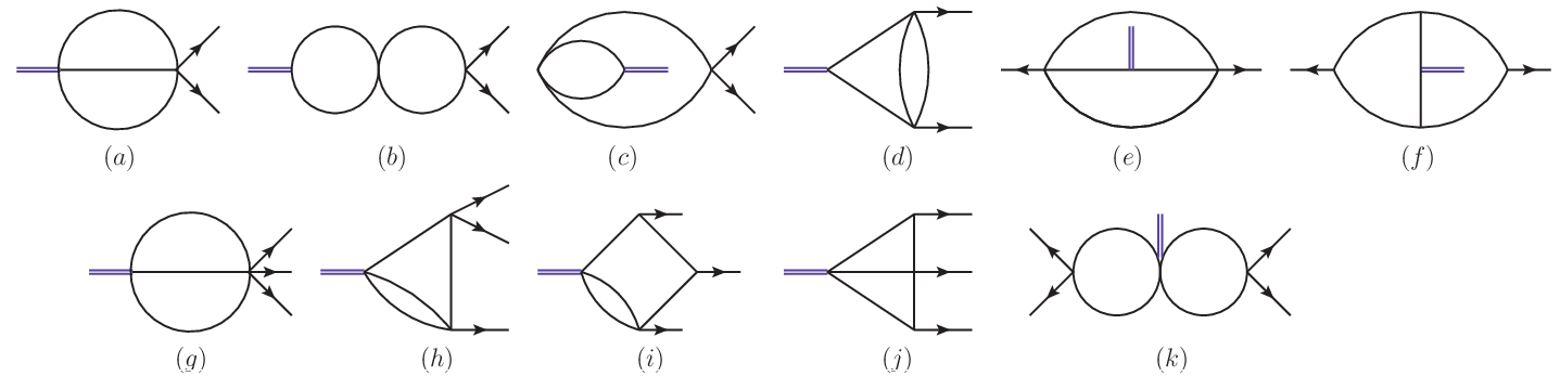
where $\mathcal{F}_{L\to n}$ represents an $n$-point form factor of a length-$L$ operator. For all these form factors, the one-loop and two-loop master integrals are shown in Figure 1 and Figure 3. And we present all corresponding cuts in Figure 2 and Figure 4. Notice that all external legs outside the loop are included in the double line. Since the calculation is in the large $N_{c}$ limit, all the cuts are planar and all the tree blocks are color-ordered. The relations between the form factors, master integrals and the cuts are as follows.

• •

  The only master for one-loop minimal form factors is $(a)$ in Figure 1, detected by the cut $(a)$ in Figure 2.

• •

  The masters for one-loop next-to-minimal form factors are $(a)\sim(c)$ in Figure 1, detected by the cuts $(a)$ and $(b)$ in Figure 2 respectively.

• •

  A two-loop sub-minimal form factor only has the master $(a)$ in Figure 3, detected by the cut $(a)$ in Figure 4.

• •

  A two-loop $2\to 2$ form factor includes the masters $(a)\sim(f)$ in Figure 3. The detecting cuts are $(a)\sim(e)$ in Figure 4. Note that since the local operator is a color singlet, the non-planar masters $(c)$, $(e)$ and $(f)$ in Figure 3 are of leading $N_{c}$ order.

• •

  A two-loop $3\to 3$ form factor includes the masters $(a),\ (b),\ (d),\ (g)\sim(j)$ in Figure 3. The flipped version of $(h)$ and $(i)$, which we do not draw, are also included in the masters. The cuts are $(a),\ (b),\ (d)$ and $(f)$ in Figure 4.

• •

  All two-loop minimal form factors with more than 3 external legs have all the masters of a two-loop $3\to 3$ form factor and the master $(k)$ in Figure 3. Accordingly, one needs one more cut, which is the cut $(g)$ in Figure 4.

It is worthwhile noting that coefficients of some master integrals can be calculated via different cuts, e.g. the master integral $(j)$ in Figure 3 can be detected by the cuts $(a)$ and $(f)$ in Figure 4. In that case, coefficients of the master integral calculated from different cuts must be the same. All two-loop master integrals can be found in Gehrmann:2000zt; Gehrmann:2001ck.

In this subsection, we give a detailed description of two methods for tensor reduction. We first introduce the gauge-invariant basis projection (see e.g. Gehrmann:2011aa; Boels:2018nrr) in Section 4.2.1. This method takes advantage of the gauge invariance of the cut form factors and is powerful for the form factors with a small number of external legs. Then in Section 4.2.2, we introduce a hybrid method, including loop momentum decomposition and the PV reductionPassarino:1978jh; Kreimer:1991wj. The second method is efficient for the calculation of the two-loop high-point form factors.

References

• (1) G. ’t Hooft and M. J. G. Veltman, Regularization and Renormalization of Gauge Fields, Nucl. Phys. B 44 (1972) 189–213.
• (2) Q. Jin, K. Ren, G. Yang, and R. Yu, Gluonic evanescent operators: classification and one-loop renormalization, arXiv:2202.08285.
• (3) A. J. Buras and P. H. Weisz, QCD Nonleading Corrections to Weak Decays in Dimensional Regularization and ’t Hooft-Veltman Schemes, Nucl. Phys. B 333 (1990) 66–99.
• (4) M. J. Dugan and B. Grinstein, On the vanishing of evanescent operators, Phys. Lett. B 256 (1991) 239–244.
• (5) S. Herrlich and U. Nierste, Evanescent operators, scheme dependences and double insertions, Nucl. Phys. B 455 (1995) 39–58, [hep-ph/9412375].
• (6) A. J. Buras, Weak Hamiltonian, CP violation and rare decays, in Les Houches Summer School in Theoretical Physics, Session 68: Probing the Standard Model of Particle Interactions, pp. 281–539, 6, 1998. hep-ph/9806471.
• (7) A. Bondi, G. Curci, G. Paffuti, and P. Rossi, Metric and Central Charge in the Perturbative Approach to Two-dimensional Fermionic Models, Annals Phys. 199 (1990) 268.
• (8) A. N. Vasiliev and M. I. Vyazovsky, Proof of the absence of multiplicative renormalizability of the Gross-Neveu model in the dimensional regularization d = 2+2epsilon, Theor. Math. Phys. 113 (1997) 1277–1288.
• (9) J. A. Gracey, T. Luthe, and Y. Schroder, Four loop renormalization of the Gross-Neveu model, Phys. Rev. D 94 (2016), no. 12 125028, [arXiv:1609.05071].
• (10) L. Di Pietro and E. Stamou, Operator mixing in the ϵ\boldsymbol{\epsilon}-expansion: Scheme and evanescent-operator independence, Phys. Rev. D 97 (2018), no. 6 065007, [arXiv:1708.03739].
• (11) M. Hogervorst, S. Rychkov, and B. C. van Rees, Unitarity violation at the Wilson-Fisher fixed point in 4-ϵ\epsilon dimensions, Phys. Rev. D 93 (2016), no. 12 125025, [arXiv:1512.00013].
• (12) W. Cao, F. Herzog, T. Melia, and J. R. Nepveu, Renormalization and non-renormalization of scalar EFTs at higher orders, JHEP 09 (2021) 014, [arXiv:2105.12742].
• (13) Z. Bern, C. Cheung, H.-H. Chi, S. Davies, L. Dixon, and J. Nohle, Evanescent Effects Can Alter Ultraviolet Divergences in Quantum Gravity without Physical Consequences, Phys. Rev. Lett. 115 (2015), no. 21 211301, [arXiv:1507.06118].
• (14) Z. Bern, H.-H. Chi, L. Dixon, and A. Edison, Two-Loop Renormalization of Quantum Gravity Simplified, Phys. Rev. D 95 (2017), no. 4 046013, [arXiv:1701.02422].
• (15) W. A. Bardeen, A. J. Buras, D. W. Duke, and T. Muta, Deep Inelastic Scattering Beyond the Leading Order in Asymptotically Free Gauge Theories, Phys. Rev. D18 (1978) 3998.
• (16) K. G. Wilson and M. E. Fisher, Critical exponents in 3.99 dimensions, Phys. Rev. Lett. 28 (1972) 240–243.
• (17) Z. Bern, L. J. Dixon, D. C. Dunbar, and D. A. Kosower, Fusing gauge theory tree amplitudes into loop amplitudes, Nucl. Phys. B435 (1995) 59–101, [hep-ph/9409265].
• (18) Z. Bern, L. J. Dixon, D. C. Dunbar, and D. A. Kosower, One loop n point gauge theory amplitudes, unitarity and collinear limits, Nucl.Phys. B425 (1994) 217–260, [hep-ph/9403226].
• (19) R. Britto, F. Cachazo, and B. Feng, Generalized unitarity and one-loop amplitudes in N=4 super-Yang-Mills, Nucl.Phys. B725 (2005) 275–305, [hep-th/0412103].
• (20) K. Chetyrkin and F. Tkachov, Integration by Parts: The Algorithm to Calculate beta Functions in 4 Loops, Nucl.Phys. B192 (1981) 159–204.
• (21) F. Tkachov, A Theorem on Analytical Calculability of Four Loop Renormalization Group Functions, Phys.Lett. B100 (1981) 65–68.
• (22) G. Passarino and M. J. G. Veltman, One Loop Corrections for e+ e- Annihilation Into mu+ mu- in the Weinberg Model, Nucl. Phys. B160 (1979) 151–207.
• (23) D. Kreimer, One loop integrals revisited. 1. The Two point functions, Z. Phys. C 54 (1992) 667–672.
• (24) G. Yang, On-shell methods for form factors in 𝒩=4\mathcal{N}=4 SYM and their applications, Sci. China Phys. Mech. Astron. 63 (2020), no. 7 270001, [arXiv:1912.11454].
• (25) W. A. Bardeen, Anomalous Ward identities in spinor field theories, Phys. Rev. 184 (1969) 1848–1857.
• (26) T. Gehrmann, M. Jaquier, E. Glover, and A. Koukoutsakis, Two-Loop QCD Corrections to the Helicity Amplitudes for H→H\to 3 partons, JHEP 1202 (2012) 056, [arXiv:1112.3554].
• (27) S. Catani, The Singular behavior of QCD amplitudes at two loop order, Phys. Lett. B427 (1998) 161–171, [hep-ph/9802439].
• (28) Q. Jin and G. Yang, Analytic Two-Loop Higgs Amplitudes in Effective Field Theory and the Maximal Transcendentality Principle, Phys. Rev. Lett. 121 (2018), no. 10 101603, [arXiv:1804.04653].
• (29) Q. Jin and G. Yang, Hidden Analytic Relations for Two-Loop Higgs Amplitudes in QCD, Commun. Theor. Phys. 72 (2020), no. 6 065201, [arXiv:1904.07260].
• (30) Q. Jin and G. Yang, Two-Loop QCD Corrections to the Higgs plus three-parton amplitudes with Top Mass Correction, JHEP 02 (2020) 169, [arXiv:1910.09384].
• (31) R. H. Boels and H. Luo, A minimal approach to the scattering of physical massless bosons, JHEP 05 (2018) 063, [arXiv:1710.10208].
• (32) R. H. Boels, Q. Jin, and H. Luo, Efficient integrand reduction for particles with spin, arXiv:1802.06761.
• (33) Q. Jin and H. Luo, Analytic Form of the Three-loop Four-gluon Scattering Amplitudes in Yang-Mills Theory, arXiv:1910.05889.
• (34) D. A. Kosower and K. J. Larsen, Maximal Unitarity at Two Loops, Phys. Rev. D85 (2012) 045017, [arXiv:1108.1180].
• (35) K. J. Larsen and Y. Zhang, Integration-by-parts reductions from unitarity cuts and algebraic geometry, Phys. Rev. D93 (2016), no. 4 041701, [arXiv:1511.01071].
• (36) H. Ita, Two-loop Integrand Decomposition into Master Integrals and Surface Terms, Phys. Rev. D94 (2016), no. 11 116015, [arXiv:1510.05626].
• (37) A. Georgoudis, K. J. Larsen, and Y. Zhang, Azurite: An algebraic geometry based package for finding bases of loop integrals, Comput. Phys. Commun. 221 (2017) 203–215, [arXiv:1612.04252].
• (38) S. Abreu, F. Febres Cordero, H. Ita, B. Page, and M. Zeng, Planar Two-Loop Five-Gluon Amplitudes from Numerical Unitarity, Phys. Rev. D 97 (2018), no. 11 116014, [arXiv:1712.03946].
• (39) S. Abreu, F. Febres Cordero, H. Ita, M. Jaquier, B. Page, and M. Zeng, Two-Loop Four-Gluon Amplitudes from Numerical Unitarity, Phys. Rev. Lett. 119 (2017), no. 14 142001, [arXiv:1703.05273].
• (40) W. Siegel, Supersymmetric Dimensional Regularization via Dimensional Reduction, Phys. Lett. B 84 (1979) 193–196.
• (41) D. M. Capper, D. R. T. Jones, and P. van Nieuwenhuizen, Regularization by Dimensional Reduction of Supersymmetric and Nonsupersymmetric Gauge Theories, Nucl. Phys. B 167 (1980) 479–499.
• (42) I. Jack, D. R. T. Jones, and K. L. Roberts, Dimensional reduction in nonsupersymmetric theories, Z. Phys. C 62 (1994) 161–166, [hep-ph/9310301].
• (43) R. Harlander, P. Kant, L. Mihaila, and M. Steinhauser, Dimensional Reduction applied to QCD at three loops, JHEP 09 (2006) 053, [hep-ph/0607240].
• (44) D. Nandan, C. Sieg, M. Wilhelm, and G. Yang, Cutting through form factors and cross sections of non-protected operators in 𝒩=4\mathcal{N}=4 SYM, JHEP 06 (2015) 156, [arXiv:1410.8485].
• (45) M. Accettulli Huber, A. Brandhuber, S. De Angelis, and G. Travaglini, Complete Form Factors in Yang-Mills from Unitarity and Spinor Helicity in Six Dimensions, Phys. Rev. D101 (2020), no. 2 026004, [arXiv:1910.04772].
• (46) J. A. Gracey, Six dimensional QCD at two loops, Phys. Rev. D93 (2016), no. 2 025025, [arXiv:1512.04443].
• (47) J. A. Gracey, Eight dimensional QCD at one loop, Phys. Rev. D97 (2018), no. 2 025009, [arXiv:1712.02565].
• (48) C. Schubert, The Yukawa Model as an Example for Dimensional Renormalization With γ\gamma (5), Nucl. Phys. B 323 (1989) 478–492.
• (49) A. V. Smirnov and F. S. Chuharev, FIRE6: Feynman Integral REduction with Modular Arithmetic, Comput. Phys. Commun. 247 (2020) 106877, [arXiv:1901.07808].
• (50) T. Gehrmann and E. Remiddi, Two loop master integrals for gamma* →\rightarrow 3 jets: The Planar topologies, Nucl. Phys. B601 (2001) 248–286, [hep-ph/0008287].
• (51) T. Gehrmann and E. Remiddi, Two loop master integrals for gamma* →\rightarrow 3 jets: The Nonplanar topologies, Nucl. Phys. B601 (2001) 287–317, [hep-ph/0101124].
• (52) J. M. Henn and J. C. Plefka, Scattering Amplitudes in Gauge Theories, vol. 883. Springer, Berlin, 2014.
• (53) J. A. Gracey, Classification and one loop renormalization of dimension-six and dimension-eight operators in quantum gluodynamics, Nucl. Phys. B634 (2002) 192–208, [hep-ph/0204266]. [Erratum: Nucl. Phys.B696,295(2004)].
• (54) A. Y. Morozov, MATRIX OF MIXING OF SCALAR AND VECTOR MESONS OF DIMENSION D <<= 8 IN QCD. (IN RUSSIAN), Sov. J. Nucl. Phys. 40 (1984) 505.
• (55) D. Neill, Two-Loop Matching onto Dimension Eight Operators in the Higgs-Glue Sector, arXiv:0908.1573.
• (56) R. V. Harlander and T. Neumann, Probing the nature of the Higgs-gluon coupling, Phys. Rev. D88 (2013) 074015, [arXiv:1308.2225].
• (57) S. Dawson, I. M. Lewis, and M. Zeng, Effective field theory for Higgs boson plus jet production, Phys. Rev. D90 (2014), no. 9 093007, [arXiv:1409.6299].
• (58) Q. Jin, K. Ren, and G. Yang, Two-Loop anomalous dimensions of QCD operators up to dimension-sixteen and Higgs EFT amplitudes, JHEP 04 (2021) 180, [arXiv:2011.02494].
• (59) V. P. Spiridonov and K. G. Chetyrkin, Nonleading mass corrections and renormalization of the operators m psi-bar psi and g**2(mu nu), Sov. J. Nucl. Phys. 47 (1988) 522–527.
• (60) A. N. Vasilev, The field theoretic renormalization group in critical behavior theory and stochastic dynamics. 2004.
• (61) T. R. Morris, Renormalizable extra-dimensional models, JHEP 01 (2005) 002, [hep-ph/0410142].
• (62) F. De Cesare, L. Di Pietro, and M. Serone, Five-dimensional CFTs from the ε\varepsilon-expansion, Phys. Rev. D 104 (2021), no. 10 105015, [arXiv:2107.00342].
• (63) J. Zinn-Justin, Quantum field theory and critical phenomena, Int. Ser. Monogr. Phys. 113 (2002) 1–1054.