Robust Causal Graph Representation Learning against Confounding Effects

IV approach (Wooldridge 2002) deals with the confounding effects by conducting estimations under conditional moment restrictions. The general type of an IV model can be described as follows. Let $X_{i}$, $Y_{i}$ denote observable variable vectors of some data distribution to be studied. $X_{i}\in\mathcal{R}^{m}$, $Y_{i}\in\mathcal{R}^{b}$. Assume that the observations $\{(X_{i},Y_{i})\}^{n}_{i=1}$ are i.i.d., our goal is to learn a structural function $f\left(\cdot\right)$ that can represent the correlations between $X_{i}$ and $Y_{i}$. We presume that $f\left(\cdot\right)$ can be completely determined by parameters $\theta^{*}$. Such a function can be formulated as:

$\displaystyle Y_{i}=f_{\theta^{*}}(X_{i}).$

(1)

Then, we can acquire $\theta^{*}$ using regression methods. Unfortunately, in real-world circumstances, confounders generally exist in the data. Formally, we have:

$\displaystyle Y_{i}=f_{\theta^{*}}(X_{i})+\epsilon_{i},$

(2)

where $\epsilon_{i}$ is the error term. If we cannot acquire a clear representation of $\epsilon_{i}$, we will not be able to get ${\theta^{*}}$ correctly according to $Y_{i}$ and $X_{i}$.

The IV approach addresses this issue with conditional moment restrictions. Such an approach selects a conditioning variables vector $Z_{i}$ as the IV. $\{(X_{i},Y_{i},Z_{i})\}^{n}_{i=1}\text{ are i.i.d.}$, $Z_{i}$ satisfies:

$\displaystyle\mathbb{E}[\epsilon_{i}|Z_{i}]=0\ \ \ \forall i\in\llbracket 1,n\rrbracket.$

(3)

By introducing $Z_{i}$ into the calculation of $f\left(\cdot\right)$, we can eliminate the confounding effects brought by $\epsilon_{i}$. Based on this idea, (Ai and Chen 2003) defines a formal training objective of the IV approach as:

$\displaystyle\mathbb{E}[f_{\theta^{*}}(X_{i})-Y_{i}|Z_{i}]=0.$

(4)

However, the IV, $Z_{i}$, is also hard to acquire in most learning tasks. In linear cases, approaches, such as (Hayashi 2000; Hansen, Heaton, and Yaron 1996), address the issue by transferring the conditional moment restrictions into unconditional ones.

Given an attributed graph $G=(V,E)$, $V$ and $E$ denote the node and edge sets, respectively. $\mathcal{G}=\left\{G_{i},i\in\llbracket{1,N^{G}}\rrbracket\right\}$ is a graph dataset. The objective of graph representation learning is to learn an encoder $f^{G}(\cdot):\mathcal{G}\to\mathbb{R}$, where $\mathbb{R}$ denotes an embedding space. Accordingly, $f^{G}(G_{i})$ is the representation containing discriminative information of $G_{i}$ for downstream tasks.

To learn the discriminative representation, benchmark methods employ GNN as the encoder. GNN encodes nodes in $G_{i}=(V_{i},E_{i})$ into embedded vectors. The $k$-th layer of GNN can be formulated as:

$$\bm{h}^{\left(k+1\right)}_{v}=\textrm{COM}^{\left(k\right)}\Bigg(\bm{h}^{\left(k\right)}_{v},\textrm{AGG}^{\left(k\right)}\left(\bm{h}^{\left(k\right)}_{u},\forall u\in\textrm{N}\left(v\right)\right)\Bigg),$$

(5)

where $\bm{h}_{v}$ denotes the vector for node $v\in V_{i}$, $\textrm{N}\left(v\right)$ denotes the neighbors of $v$, and $\bm{h}^{\left(k\right)}$ is the representation vector of the corresponding node at the $k$-th layer. Specifically, $\bm{h}^{\left(0\right)}$ is initialized with the input node features. $\textrm{COM}\left(\cdot\right)$ and $\textrm{AGG}\left(\cdot\right)$ are learnable functions of GNN. $\textrm{COM}\left(\cdot\right)$ combines the aggregated neighbor feature into the feature of the target node, and $\textrm{AGG}\left(\cdot\right)$ aggregates the features of neighbors. To obtain the graph representation $f^{G}(G_{i})$ for $G_{i}$, we adopt

$${f^{G}(G_{i})}=\textrm{READOUT}\left(\bm{h}_{v},v\in V_{i}\right),$$

(6)

where $\textrm{READOUT}\left(\cdot\right)$ is a readout function pooling the node representations $\left\{\bm{h}_{v}|v\in V_{i}\right\}$.

Our method aims at enhancing causality in graph representation learning. We propose that models generating predictions with high causal relationships with labels can be treated as “confounder-robust” models. We define a confounder-robust GNN as follows.

We adopt the IV approach (Greene 2003) to empower us to acquire a confounder-robust model. Given a graph dataset $\mathcal{G}=\left\{G_{i},i\in\llbracket{1,N^{G}}\rrbracket\right\}$, we define the confounder in each graph as $C_{i}$. Meanwhile, $X_{i}$ denotes the information causally related to $Y_{i}$. However, $X_{i}$ and $C_{i}$ are mixed in $G_{i}$. Our purpose is to train a GNN model to predict the label $Y_{i}$ based on $X_{i}$, regardless of $C_{i}$. We denote the parameter of the model that can achieve such a goal as $\theta^{*}$. With the IV approach, our objective is to acquire $\theta^{*}$, which can be formulated as follows.

	$$\displaystyle\theta^{*}=\arg\min_{\theta}\Big(\mathbb{E}[m(G_{i},Y_{i},Z_{i},\theta)|Z_{i}]\Big),\forall i\in\llbracket 1,n\rrbracket$$
	$$\displaystyle s.t.\ \mathbb{E}[(|C_{i}|)|Z_{i}]=0,\ \forall i\in\llbracket 1,n\rrbracket,$$		(7)

where $m(\cdot)$ outputs the difference between the model’s output and ground truth labels, $|C_{i}|$ denotes the number of elements in $C_{i}$, $Z_{i}$ denote the IVs that instruct the model to eliminate confounders $C_{i}$ through certain measures. Equation 7 can be treated as a generalization of Equation 4 in the field of graph representation learning.

As mentioned above, the IV $Z_{i}$ can be challenging to acquire. Furthermore, the complexity of graph representation learning with neural networks enlarges such difficulty. To make calculating $Z_{i}$ operable, we transfer the conditional moment restrictions of Equation 7 into unconditional moment restrictions by generating the IV $Z_{i}$ with a GNN model $q^{G}(\cdot)$, which can be formulated as:

$\displaystyle Z_{i}=q^{G}_{\varphi}(G_{i}),$

(8)

where $\varphi$ are the parameters of GNNs that generates $Z_{i}$. To replace $Z_{i}$, an ideal $q^{G}(\cdot)$ with parameters $\varphi^{*}$ should satisfy:

$\displaystyle\mathbb{E}[(|C_{i}|)|q^{G}_{\varphi^{*}}(G_{i})]=0,\ \ \ \forall i\in\llbracket 1,n\rrbracket.$

(9)

As we expect to train the model to predict the label $Y_{i}$ based on $X_{i}$, we need to leave $X_{i}$ unaffected. Therefore, $q^{G}(\cdot)$ should also satisfy:

$\displaystyle\mathbb{E}[X_{i}|q^{G}_{\varphi^{*}}(G_{i})]=X_{i},\ \ \ \forall i\in\llbracket 1,n\rrbracket.$

(10)

As $q^{G}(\cdot)$ is a GNN, we can utilize the backpropagation to train it. We propose the following theorem to define the objective for training $q^{G}(\cdot)$.

Proof. We provide proofs to demonstrate the effectiveness of Theorem 1. Since we already know the values of $\theta^{*}$, therefore, $\varphi^{*}$ is the only parameter variable in Equation 11. We can give the proof of Theorem 1 by proofing that equations 9 and 10 hold if and only if cross entropy $I\big(f_{\theta^{*}}^{G}(r(G,q^{G}_{\varphi^{*}}(G))),Y\big)$ reaches the maximum value.

First, we prove the sufficiency. According to the definition of mutual information, we have:

	$$\displaystyle I\left(f_{\theta^{*}}^{G}\left(r\left(G,q^{G}_{\varphi^{*}}(G)\right)\right),Y\right)=$$
	$$\displaystyle H(Y)-H\left(Y|f_{\theta^{*}}^{G}\left(r\left(G,q^{G}_{\varphi^{*}}(G)\right)\right)\right).$$		(12)

$H(Y)$ is defined by the distribution of the dataset, therefore $H(Y)$ has a fixed value. Thus, if $I\left(f_{\theta^{*}}^{G}\left(r\left(G,q^{G}_{\varphi^{*}}(G)\right)\right),Y\right)$ reaches maximum, then $H\left(Y|f_{\theta^{*}}^{G}\left(r\left(G,q^{G}_{\varphi^{*}}(G)\right)\right)\right)$ reaches minimum, i.e., $H\left(Y|f_{\theta^{*}}^{G}\left(r\left(G,q^{G}_{\varphi^{*}}(G)\right)\right)\right)=0$. Therefore, according to the definition of conditional entropy, we have:

	$$\displaystyle H\left(Y|f_{\theta^{*}}^{G}\left(r\left(G,q^{G}_{\varphi^{*}}(G)\right)\right)\right)$$
	$$\displaystyle=-\mathbb{E}\Big[log\Big(p\left(Y|f_{\theta^{*}}^{G}\left(r\left(G,q^{G}_{\varphi^{*}}(G)\right)\right)\right)\Big)\Big]=0$$		(13)

As $log\Big(p\left(Y_{i}|f_{\theta^{*}}^{G}\left(r\left(G_{i},q^{G}_{\varphi^{*}}(G_{i})\right)\right)\right)\Big)\leq 0$, if the above equation holds, then:

	$$\displaystyle log\Big(p\left(Y_{i}|f_{\theta^{*}}^{G}\left(r\left(G_{i},q^{G}_{\varphi^{*}}(G_{i})\right)\right)\right)\Big)=0$$
	$$\displaystyle,i=1,2,3,...,n.$$		(14)

Therefore, we have:

	$$\displaystyle p\left(Y_{i}|f_{\theta^{*}}^{G}\left(r\left(G_{i},q^{G}_{\varphi^{*}}(G_{i})\right)\right)\right)=1$$
	$$\displaystyle,i=1,2,3,...,n.$$		(15)

As $f(\cdot)$ output the prediction of $Y$, thus, we have:

$$\displaystyle Y_{i}=f_{\theta^{*}}^{G}\left(r\left(G_{i},q^{G}_{\varphi^{*}}(G_{i})\right)\right),i=1,2,3,...,n.$$

(16)

According to the assumptions, the following equation holds:

$$\displaystyle Y_{i}=f_{\theta^{*}}^{G}(X_{i}),i=1,2,3,...,n.$$

(17)

And, $f^{G}_{\theta^{*}}(X_{i}\cup C^{\prime}_{i})\neq Y_{i},\forall C^{\prime}_{i}\subseteq C_{i}$, therefore:

$$\displaystyle r\left(G_{i},q^{G}_{\varphi^{*}}(G_{i})\right)=X_{i},i=1,2,3,...,n.$$

(18)

As $r(\cdot)$ is a non-parameter function that removes graph data according to $q(\cdot)$, according to Equation 18, the confounder $C_{i}$ has been totally removed and the information of $X_{i}$ is unaffected. Therefore, the conditions defined in Equations 9 and 10 are met. Then, we can get that if $I\left(f_{\theta^{*}}^{G}\left(r\left(G,q^{G}_{\varphi^{*}}(G)\right)\right),Y\right)$ is maximized, then Equations 9 and 10 holds, the sufficiency is proved.

Next, we will prove the necessity. If Equations 9 and 10 hold, then $r(\cdot)$ will be able to remove $C_{i}$ without affecting $X_{i}$, therefore Equation 18 holds. Substituting Equation 18 into Equation 12, we get:

	$$\displaystyle I\left(f_{\theta^{*}}^{G}\left(r\left(G,q^{G}_{\varphi^{*}}(G)\right)\right),Y\right)=$$
	$$\displaystyle I\left(f_{\theta^{*}}^{G}\left(X_{i}\right),Y\right)=H(Y)-H\left(Y|f_{\theta^{*}}^{G}\left(X_{i}\right)\right).$$		(19)

As $Y_{i}=f^{G}_{\theta^{*}}(X_{i})$, we have:

$$\displaystyle I\left(f_{\theta^{*}}^{G}\left(r\left(G,q^{G}_{\varphi^{*}}(G)\right)\right),Y\right)=H(Y)-H(Y|Y).$$

(20)

Because $H(Y|Y)=0$, therefore $I\left(f_{\theta^{*}}^{G}\left(r\left(G,q^{G}_{\varphi^{*}}(G)\right)\right),Y\right)$ is maximized. We can then come up with the conclusion that if Equation 9 and Equation 10 holds, then $I\left(f_{\theta^{*}}^{G}\left(r\left(G,q^{G}_{\varphi^{*}}(G)\right)\right),Y\right)$ is maximized. The necessity is proved.

With the sufficiency and necessity proved, we can say that Equations 9 and 10 holds if and only if cross entropy $H\big(f_{\theta^{*}}^{G}(r(G,q^{G}_{\varphi^{*}}(G))),Y\big)$ reaches the minimum value. According to the discussion at the beginning of the proof, we have proved Theorem 1.

With Equation 7 and Theorem 1, we define our IV approach-based training objective with unconditional moment restrictions as:

$$\displaystyle\theta^{*}=\arg\min_{\theta}\Big(\mathbb{E}[m(G_{i},Y_{i},q_{\varphi^{*}}^{G}(G_{i}),\theta)]\Big),$$

(21)

where $\varphi^{*}$ can be calculated with Equation 11. However, at the beginning, we can neither acquire $\theta^{*}$ nor $\varphi^{*}$. Furthermore, the assumptions of Theorem 1 cannot be strictly met in real-world scenarios. To address such issues, we initialize $\theta$ and $\varphi$ randomly and update them alternatively. We further introduce some new designs to ensure that the model can learn label-causal-related graph representations against confounding effects. These designs will be discussed in the implementation and optimization parts.

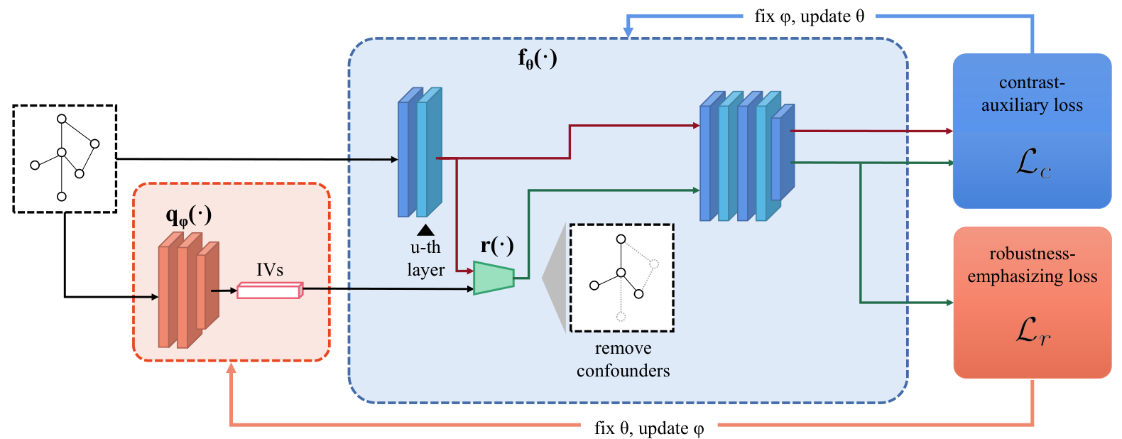
We implement the framework to reach the training objectives defined in Equations 11 and 21. See Figure 3 for the illustration. We build a GNN $f^{G}(\cdot)$ as our encoder, and a GNN $q^{G}(\cdot)$, which outputs the IVs as a series of edge weights. These edge weights are used to remove a certain amount of graph data, including dropping certain edges when the corresponding edge weights are too low and reducing information transfer through edges according to the edge weights.

Meanwhile, some nodes and edges may contain both causal and confounding information. Certain critical information may be lost if they are removed before went through the GNN encoder. Therefore, we perform graph data removal after the $u$-th layer of $f^{G}(\cdot)$, $u$ is a hyperparameter. In this way, We can perform confounder elimination at a more fine-grained level.

To make $f^{G}(\cdot)$ further robust to confounders, we introduce the concept of contrastive learning into our network. We enforce the encoder without the confounder removed to output similar features as the original ones (with the confounder removed), thereby bootstrapping the encoder’s ability to eliminate the confounding effects of some confounders.

For optimization, we perform the updates alternatively, i.e., fix $\theta$ to learn $\varphi$, and then fix $\varphi$ to learn $\theta$, and so on. We update the parameter $\varphi$ of $q^{G}(\cdot)$ according to Theorem 1, and maximize $I\left(f_{\theta^{*}}^{G}\left(r\left(G,q^{G}_{\varphi}(G)\right)\right),Y\right)$ in Equation 11 by minimizing the cross entropy loss based on the label and the model output.

Our confounder elimination operation should be beneficial to improve the causality of model predictions. Therefore, in order to get a more ideal $\varphi$, we need to further optimize the training of $q^{G}(\cdot)$ from the causality aspect. According to Definition 1, a confounder-robust GNN model is required to make correct predictions regardless of the confounders. Based on this, the model should learn the same representations for the same and correct category. For the graph sample $G_{i}$ of class $l$, suppose the model learns a representation vector $\bm{h}_{i}$, and $\bm{h}_{i}$ enables the model to perform the correct prediction. Then, the optimal value of $\bm{h}_{i}$ is to be the same as other representation vectors within the same class $l$. On the other hand, if $\bm{h}_{i}$ fails to enable the model to predict correctly, $\bm{h}_{i}$ is restricted to be different from all other classification feature vectors within class $l$. According to (Sun et al. 2020), the farther the output deviates from the optimal value, the greater the contribution to training. Inspired by such intuition, during the optimization of $q^{G}(\cdot)$, we want to emphasize those samples that contribute more to training in terms of causality.

Specifically, for $\bm{h}_{i}$ belongs to class $l$, we first obtain a feature vector $\bm{t}_{i}$, which is the average of all feature vectors within the class $l$. Then, we acquire a series of weights $w_{i}$ for samples to perform the emphasizing operation, which is formulated by:

$$\displaystyle w_{i}=\begin{split}\left\{\begin{array}[]{lr}|s(\bm{h}_{i},\bm{t}_{i})-O_{max}|,&\text{correct result,}\\ |s(\bm{h}_{i},\bm{t}_{i})-O_{min}|,&\text{wrong result,}\\ \end{array}\right.\end{split}$$

(22)

where $s(\cdot)$ stands for the similarity calculation function, $O_{min}$ and $O_{max}$ denote the minimal and maximal values of similarity, respectively.

We can then define the loss for learning $\varphi$:

$$\displaystyle\mathcal{L}_{w}=\frac{1}{n}\sum_{i=1}^{n}w_{i}^{\gamma}\mathcal{H}\Big(f^{G}_{\dot{\theta}}\big(r(G_{i},q^{G}_{\varphi}(G_{i}))\big),Y_{i}\Big),$$

(23)

where $\mathcal{H}(\cdot)$ calculates the cross entropy loss for the $i$-th sample. $n$ is the amount of samples. $\dot{\theta}$ denotes the fixed parameters of $f^{G}(\cdot)$. $\gamma$ is a hyperparameter that controls the effect of $w_{l,i}$.

$\mathcal{L}_{w}$ makes the model output more consistent representations for the same class. We further hope that the representations of all the samples be discriminative and that the model can distinguish the samples of different classes. Therefore, we design a regular term $\mathcal{M}$:

$$\displaystyle\mathcal{M}=\tau\frac{1}{n}\sum_{i=1}^{n}|s(\bm{h}_{i},\bar{\bm{t}})-O_{max}|,$$

(24)

where $\bar{\bm{t}}$ denotes the average of all feature vectors of all classes. $\tau$ is a hyperparameter. $\mathcal{M}$ prevents the model from outputting the same features for all classes, or, falling into a local optimum as parts of the graph data are removed according to the proposed IV-based approach.

Leveraging Equations 23 and 24, we propose the robustness-emphasizing loss for learning $\varphi$:

$$\displaystyle\mathcal{L}_{r}=\mathcal{L}_{w}+\zeta\mathcal{M},$$

(25)

where $\zeta$ can be defined as follows:

$$\displaystyle\zeta=\begin{split}\left\{\begin{array}[]{lr}-1,&\mathcal{M}\leq\sigma\\ 0,&\mathcal{M}>\sigma.\\ \end{array}\right.\end{split}$$

(26)

$\sigma$ is the hyperparameter that determines when the regular term $\mathcal{M}$ should be activated.

For the optimization of $\theta$, our objective is defined in Equation 21. As an implementation for $m(\cdot)$ in Equation 21, we adopt the cross entropy loss to judge the difference between model output and ground truth labels. Formally, we define the loss for learning $\theta$ as:

$$\displaystyle\mathcal{L}_{o}=\frac{1}{n}\sum_{i=1}^{n}\mathcal{H}\Big(f^{G}_{\theta}\big(r(G_{i},q^{G}_{\dot{\varphi}}(G_{i}))\big),Y_{i}\Big),$$

(27)

where $\dot{\varphi}$ denotes the fixed parameters of $q^{G}(\cdot)$. Moreover, we build a contrastive structure to make $f^{G}(\cdot)$ further robust to confounders. For the training objective, we design a contrastive loss as follows:

$$\displaystyle\mathcal{L}_{a}=-\frac{1}{n}\sum_{i=1}^{n}s\Big(f^{G}_{\dot{\theta}}\big(r(G_{i},q^{G}_{\dot{\varphi}}(G_{i}))\big),f^{\prime G}_{\theta}\big(G_{i}\big)\Big),$$

(28)

where $s(\cdot)$ denotes the similarity calculation function, $\dot{\varphi}$ denotes the fixed parameters of $q^{G}(\cdot)$, and $f^{\prime G}(\cdot)$ denotes the encoder without the confounder removal module.

Note that $f^{\prime G}(\cdot)$ and $f^{G}(\cdot)$ share the same GNN structure and parameters, but the parameters of $f^{G}(\cdot)$ are fixed as $\dot{\theta}$, i.e., $f^{G}(\cdot)$ are excluded from back propagation of $\mathcal{L}_{a}$. Therefore, $f^{\prime G}(\cdot)$ that fed by the input data containing confounders is enforced to generate similar outputs as $f^{G}(\cdot)$, which fed by the graphs without confounders (by using the confounder removal operation). Then, the learned parameters of $f^{\prime G}(\cdot)$ will be used to update $f^{G}(\cdot)$. This training paradigm encourages $f^{\prime G}(\cdot)$ to ignore information with confounding effects, result in certain confounders no longer have confounding effects on our model. Because we fix the outputs of a view in the contrastive learning part, we could avoid the risk of generating trivial solutions. Therefore, the contrastive learning in our method can be performed without negative samples, which significantly simplifies the computation during training.

We combine Equations 27 and 28 to introduce the contrast-auxiliary loss as the training objective of $\theta$:

$$\displaystyle\mathcal{L}_{c}=\mathcal{L}_{o}+\lambda\mathcal{L}_{a},$$

(29)

where $\lambda$, as a hyperparameter, controls the effect of $\mathcal{L}_{a}$.

We evaluate our method on both OOD and ID datasets. The OOD datasets include: 1) Spurious-Motif, a synthetic dataset created by (Ying et al. 2019), and we adopt the re-implementation version created by (Wu et al. 2022); 2) Graph-SST2(OOD) is an OOD version of Graph-SST2 (Yuan et al. 2020) created by (Wu et al. 2022). The ID datasets include: Graph-SST2 (ID) (Yuan et al. 2020), Graph-Twitter (Yuan et al. 2020), Mol-BBBP, and Mol-BACE (Hu et al. 2020). Different GNNs are picked for different datasets. Please refer to Appendix A for details.

We compare our method with Empirical Risk Minimization (ERM) and various causality-enhanced methods, including the interpretable baselines, i.e., GAT and Top-k Pool, and the robust learning baselines, i.e., Group DRO, IRM, and DIR.

For a fair comparison, we follow the experimental principle of (Wu et al. 2022) and adopt the same training setting for all models, which is described in detail in Appendix A. For each task, we report the averaged performance $\pm$ std over ten runs. Some of the results are cited from (Wu et al. 2022). For the values of the hyperparameters, please refer to Appendix A.3. To study the effects of the weights $w$ and contrastive loss $\mathcal{L}_{a}$, we create two additional ablation models by dropping certain structures. The first one is RCGRL-Wabl, which removes the weight factor $w$. The second one is RCGRL-Labl, which removes the contrastive loss $\mathcal{L}_{a}$. We train RCGRL-Wabl and RCGRL-Labl under the same training setting.

The results are reported in Table 1 and 2. We observe from the tables and find that our method outperforms all baselines on all downstream tasks, which demonstrates that RCGRL can learn discriminative and robust graph representations against confounding effects. Such representations have the desired performance on both ID and OOD problems, i.e., RCGRL has outstanding prediction performance and generalization ability. For the ablation studies, RCGRL outperforms RCGRL-Wabl and RCGRL-Labl on most tasks, which verifies the effectiveness of our proposed weights $w$ and auxiliary contrastive learning.

References

- Ai and Chen (2003) Ai, C.; and Chen, X. 2003. Efficient estimation of models with conditional moment restrictions containing unknown functions. Econometrica, 71(6): 1795–1843.
- Arjovsky et al. (2019) Arjovsky, M.; Bottou, L.; Gulrajani, I.; and Lopez-Paz, D. 2019. Invariant risk minimization. arXiv preprint arXiv:1907.02893.
- Gao and Ji (2019a) Gao, H.; and Ji, S. 2019a. Graph U-Nets. In Chaudhuri, K.; and Salakhutdinov, R., eds., Proceedings of the 36th International Conference on Machine Learning, ICML 2019, 9-15 June 2019, Long Beach, California, USA, volume 97 of Proceedings of Machine Learning Research, 2083–2092. PMLR.
- Gao and Ji (2019b) Gao, H.; and Ji, S. 2019b. Graph u-nets. In international conference on machine learning, 2083–2092. PMLR.
- Glymour, Pearl, and Jewell (2016) Glymour, M.; Pearl, J.; and Jewell, N. P. 2016. Causal inference in statistics: A primer. John Wiley & Sons.
- Greene (2003) Greene, W. H. 2003. Econometric analysis. Pearson Education India.
- Hansen, Heaton, and Yaron (1996) Hansen, L. P.; Heaton, J.; and Yaron, A. 1996. Finite-sample properties of some alternative GMM estimators. Journal of Business & Economic Statistics, 14(3): 262–280.
- Hayashi (2000) Hayashi, F. 2000. Econometrics,‖ Princeton University Press: Princeton.
- Hu et al. (2021) Hu, W.; Fey, M.; Ren, H.; Nakata, M.; Dong, Y.; and Leskovec, J. 2021. OGB-LSC: A Large-Scale Challenge for Machine Learning on Graphs. In Vanschoren, J.; and Yeung, S., eds., Proceedings of the Neural Information Processing Systems Track on Datasets and Benchmarks 1, NeurIPS Datasets and Benchmarks 2021, December 2021, virtual.
- Hu et al. (2020) Hu, W.; Fey, M.; Zitnik, M.; Dong, Y.; Ren, H.; Liu, B.; Catasta, M.; and Leskovec, J. 2020. Open graph benchmark: Datasets for machine learning on graphs. Advances in neural information processing systems, 33: 22118–22133.
- Kipf and Welling (2016) Kipf, T. N.; and Welling, M. 2016. Semi-supervised classification with graph convolutional networks. arXiv preprint arXiv:1609.02907.
- Krueger et al. (2021) Krueger, D.; Caballero, E.; Jacobsen, J.-H.; Zhang, A.; Binas, J.; Zhang, D.; Le Priol, R.; and Courville, A. 2021. Out-of-distribution generalization via risk extrapolation (rex). In International Conference on Machine Learning, 5815–5826. PMLR.
- Lee, Lee, and Kang (2019) Lee, J.; Lee, I.; and Kang, J. 2019. Self-Attention Graph Pooling. In Chaudhuri, K.; and Salakhutdinov, R., eds., Proceedings of the 36th International Conference on Machine Learning, ICML 2019, 9-15 June 2019, Long Beach, California, USA, volume 97 of Proceedings of Machine Learning Research, 3734–3743. PMLR.
- Li, Ren, and Li (2014) Li, H.; Ren, C.; and Li, L. 2014. U-processes and preference learning. Neural computation, 26(12): 2896–2924.
- Lin, Lan, and Li (2021) Lin, W.; Lan, H.; and Li, B. 2021. Generative Causal Explanations for Graph Neural Networks. In Proceedings of the 38th International Conference on Machine Learning, ICML 2021, 18-24 July 2021, Virtual Event, Proceedings of Machine Learning Research. PMLR.
- Luo et al. (2020) Luo, D.; Cheng, W.; Xu, D.; Yu, W.; Zong, B.; Chen, H.; and Zhang, X. 2020. Parameterized explainer for graph neural network. Advances in neural information processing systems, 33: 19620–19631.
- Morris et al. (2019) Morris, C.; Ritzert, M.; Fey, M.; Hamilton, W. L.; Lenssen, J. E.; Rattan, G.; and Grohe, M. 2019. Weisfeiler and Leman Go Neural: Higher-Order Graph Neural Networks. In The Thirty-Third AAAI Conference on Artificial Intelligence, AAAI 2019, The Thirty-First Innovative Applications of Artificial Intelligence Conference, IAAI 2019, The Ninth AAAI Symposium on Educational Advances in Artificial Intelligence, EAAI 2019, Honolulu, Hawaii, USA, January 27 - February 1, 2019, 4602–4609. AAAI Press.
- Ranjan, Sanyal, and Talukdar (2020) Ranjan, E.; Sanyal, S.; and Talukdar, P. P. 2020. ASAP: Adaptive Structure Aware Pooling for Learning Hierarchical Graph Representations. In The Thirty-Fourth AAAI Conference on Artificial Intelligence, AAAI 2020, The Thirty-Second Innovative Applications of Artificial Intelligence Conference, IAAI 2020, The Tenth AAAI Symposium on Educational Advances in Artificial Intelligence, EAAI 2020, New York, NY, USA, February 7-12, 2020, 5470–5477. AAAI Press.
- Sagawa et al. (2019) Sagawa, S.; Koh, P. W.; Hashimoto, T. B.; and Liang, P. 2019. Distributionally Robust Neural Networks. In International Conference on Learning Representations.
- Sun et al. (2020) Sun, Y.; Cheng, C.; Zhang, Y.; Zhang, C.; Zheng, L.; Wang, Z.; and Wei, Y. 2020. Circle loss: A unified perspective of pair similarity optimization. In Proceedings of the IEEE/CVF Conference on Computer Vision and Pattern Recognition, 6398–6407.
- Veličković et al. (2017) Veličković, P.; Cucurull, G.; Casanova, A.; Romero, A.; Lio, P.; and Bengio, Y. 2017. Graph attention networks. arXiv preprint arXiv:1710.10903.
- Wooldridge (2002) Wooldridge, J. M. 2002. Econometric analysis of cross section and panel data MIT press. Cambridge, MA, 108(2): 245–254.
- Wu et al. (2022) Wu, Y.-X.; Wang, X.; Zhang, A.; He, X.; and Chua, T.-S. 2022. Discovering invariant rationales for graph neural networks. arXiv preprint arXiv:2201.12872.
- Xu et al. (2018) Xu, K.; Hu, W.; Leskovec, J.; and Jegelka, S. 2018. How Powerful are Graph Neural Networks? In International Conference on Learning Representations.
- Ying et al. (2019) Ying, Z.; Bourgeois, D.; You, J.; Zitnik, M.; and Leskovec, J. 2019. /Gnnexplainer: Generating explanations for graph neural networks. Advances in neural information processing systems, 32.
- Yuan et al. (2020) Yuan, H.; Yu, H.; Gui, S.; and Ji, S. 2020. Explainability in graph neural networks: A taxonomic survey. arXiv preprint arXiv:2012.15445.
- Yuan et al. (2021) Yuan, H.; Yu, H.; Wang, J.; Li, K.; and Ji, S. 2021. On explainability of graph neural networks via subgraph explorations. In International Conference on Machine Learning, 12241–12252. PMLR.