Bayesian Latent Variable Co-kriging Model in Remote Sensing for Observations with Quality Flagged

Remote sensing technology provides a wealth of information for understanding geophysical processes with unprecedented spatial and temporal coverage. Remote sensing data provide indirect information on these geophysical quantities of interest, which are typically estimated or inferred from instrument spectra (Susskind et al. 2003). The heterogeneous nature of the Earth’s atmosphere and surface contributes to remote sensing data records with variable quality, which is often documented by the product development teams and included as quality flags associated with observations in remote sensing data products (Thrastarson et al. 2021, e.g.,). These quality flags, instead of providing quantitative uncertainty measures for the observations, indicate whether data are of good, acceptable or unreliable qualities. When the remote sensing data products are used in a wide range of downstream analyses, these quality flags are usually treated in a dichotomous way: Data flagged as unreliable are removed, while the remaining data, no matter how they may be flagged differently (e.g., good or acceptable), are combined directly (Zhu et al. 2015; Ma and Kang 2020b; Tian et al. 2020; Waliser et al. 2020, e.g.,). This practice ignores the delicate quality difference between observations with different quality flags.

Our work is motivated by data products from the Atmospheric Infrared Sounder (AIRS) instrument on board NASA’s Aqua satellite. The AIRS instrument collects radiance spectra, termed Level 1 data products, across the globe in the infrared portion of the spectrum. A retrieval algorithm is used to infer atmospheric quantities such as temperature and humidity from the spectra at 45km$\mathchar 8706$ 45km spatial resolution, called the Level 2 data products (Susskind et al. 2003). Note that the AIRS Level 2 data products include a quality flag (QF) variable: QF value of $\mathchar 28720$ indicates observations of very good quality, QF value of $\mathchar 28721$ indicates observations of acceptable quality, and QF value of $\mathchar 28722$ are deemed to be bad or unreliable. AIRS data products have been used by weather prediction centers around the world to improve weather forecasts (Lu and Zhang 2019). They are also used to assess the skill of climate models and in applications ranging from volcanic plume detection (Prata and Lynch 2019) to drought forecasting (Behrangi et al. 2016). Although data with QF value of 0 are removed from such analyses, AIRS data with QF values of 1 and 0 are combined without further consideration of their quality difference indicated by their QF values (Tian et al. 2020; Waliser et al. 2020, e.g.,). In this work, we focus on ARIS Level 2 air temperature data at 100 different vertical pressure levels which we refer to as 3D (longitude, latitude, and vertical atmospheric pressure level) air temperature observations. To our knowledge, our work is the first to build a statistical model for such quality-flagged remote sensing data.

Since the quality flags indicate variable fidelity associated with remote sensing observations, a natural statistical model to explore the dependencies of successive fidelity levels is the autoregressive co-kriging model (Kennedy and O’Hagan 2000). Essentially, this autoregressive co-kriging method considers a scalar and an additive discrepancy to model observations with a sequential fidelity order. A number of important variations of this model have been proposed. Qian and Wu 2008 consider the scale discrepancy as a function of the input space by casting it as a Gaussian process (GP) which produces non-standard conditional posteriors. Perdikaris et al. 2017 relax the auto-regressive structure by using deep learning ideas to introduce nonlinear relationships, but the computational cost to train the model is significantly increased. Konomi and Karagiannis 2021 propose a Bayesian augmented hierarchical co-kriging procedure which makes possible the analysis of non-nested input and non-stationary output. These methods rely on Gaussian processes and do not scale well with large data sets. Meanwhile, these methods are initially designed for deterministic computer models and thus don’t include a term for measurement errors which is highly recommended in spatial statistics (Cressie 1993; Stein 1999).

Spatial statistical methods for big data have been evolving over the past two decades due to emergence of massive spatial data sets. Banerjee 2017 and Heaton et al. 2019 provide a good overview of these methods with comparisons. Briefly we distinguish between low-rank approximation methods (Banerjee et al. 2008; Cressie and Johannesson 2008), approximate likelihood methods (Stein et al. 2004; Gramacy and Apley 2015), sparse structures (Lindgren et al. 2011; Nychka et al. 2015; Ma and Kang 2020a; Peruzzi et al. 2020), multiple-scale approximation (Sang and Huang 2012; Katzfuss 2017), and lower dimensional conditional distributions (Vecchia 1988; Stein et al. 2004; Datta et al. 2016; Katzfuss and Guinness 2021). Directly applying these methods within the autoregressive co-kriging framework for multi-fidelity remote sensing data is complicated. In particular, when the locations of data at different fidelity levels are not nested, the likelihood function no longer benefits from the Markovian property assumed in the model, making it complex to apply the methods aforementioned for massive spatial data (Konomi and Karagiannis 2021). Recently, Cheng et al. 2021 extend the nearest-neighbor Gaussian process (NNGP) to analyze multi-level data sets by introducing a nested NNGP reference set for each level. Although this method can handle multi-fidelity data, its way to define the reference sets makes it more appropriate when low-fidelity data are observed homogeneously over the spatial domain, but not suitable for the AIRS data described in Section 2 when the observations with the same QF values are clustered spatially.

In this paper, we propose a latent variable co-kriging model with separable Gaussian processes, which is able to account for multi-fidelity remote sensing data with measurement errors. Noticing that for AIRS Level 2 data products the latitude and longitude of observation locations are fixed across different vertical pressure levels, we adopt a multiplicative (separable) covariance function for the horizontal and vertical dimensions. Such a multiplicative (separable) covariance function is widely used in spatial statistics (Banerjee et al. 2014) and uncertainty quantification for computer experiments (Gramacy 2020). For AIRS air temperature data, the resulting covariance matrix can be decomposed into a Kronecker product of a purely horizontal (i.e., latitude and longitude) correlation matrix and a purely vertical (i.e., pressure level) correlation matrix. This can alleviate the computational bottleneck related to Gaussian process likelihood evaluation and spatial prediction (Genton 2007; Rougier 2008; Bilionis et al. 2013; Guillas et al. 2018; Ma et al. 2019). However, the introduction of the different QF values as well as missing data destroys this Kronecker-product representation of the separable covariance structure. To facilitate efficient inference, we introduce an imputation mechanism within the Markov chain Monte Carlo (MCMC) procedure to take advantage of the latent variable representation and the data structure, which enables us to decompose the large covariance matrices into two separate computationally efficient components. Moreover, we propose a computationally efficient Monte Carlo recursive prediction procedure to make spatial prediction at high-fidelity level. We apply this proposed method to analyze level 2 AIRS air temperature data. Extensive numerical results demonstrate that compared to methods that ignores the different QF values of data, our method provides more accurate predictions but also remains computationally efficient.

The rest of the paper is organized as follows. In Section 2, we introduce the quality-flagged AIRS 3D air temperature data studied in this work. Section 3 presents the latent variable co-kriging model. In Section 4, we give details on Bayesian inference including spatial prediction by constructing an augmented posterior using imputation of latent variables. In Section 5, we apply the proposed method to analyze the AIRS air temperature data and demonstrate its inferential advantages compared to methods ignoring the quality flags. We offer conclusions and discussion in Section 6.

The Atmospheric Infrared Sounder (AIRS) instrument on board NASA’s Aqua satellite measures radiance spectra in infrared channels along the satellite’s polar orbit. These infrared channels are sensitive to thermal emission from the atmosphere. The AIRS retrieval algorithm first obtains cloud properties and effective cloud-cleared radiance (CCR) and then uses CCR to further infer atmospheric properties including temperature and humidity at different vertical pressure levels at 45km $\mathchar 8706$ 45km spatial resolution. A single 45km $\mathchar 8706$ 45km areal unit is known as a field of regard (FOR) in Susskind et al. 2003. AIRS Level 2 data are further sectioned into pieces called granules. Each granule is roughly 2250km $\mathchar 8706$ 1650km and thus contains $\mathchar 29038_{\mathchar 29043}\mathchar 12349\mathchar 28721\mathchar 28723\mathchar 28725\mathchar 28720$ FORs horizontally at each pressure level. Tere are a total of $\mathchar 29038_{\mathchar 29040}\mathchar 12349\mathchar 28721\mathchar 28720\mathchar 28720$ pressure levels in AIRS data products. Therefore, Within a granule, there are potentially $\mathchar 28721\mathchar 24891\mathchar 28723\mathchar 28725\mathchar 28720\mathchar 8706\mathchar 28721\mathchar 28720\mathchar 28720\mathchar 12349\mathchar 28721\mathchar 28723\mathchar 28725\mathchar 24891\mathchar 28720\mathchar 28720\mathchar 28720$ in the three-dimensional domain (horizontally and vertically).

It has been noted that heterogeneity of clouds yields substantial variability in the radiance, resulting in varying quality of the retrievals. Therefore, most retrieved remote sensing data for atmospheric properties including air temperature are accompanied by a quality flag (QF) variable. The AIRS convention is that QF values of 0 indicate best quality data, mostly retrieved under a clear-sky condition, values of 1 indicate acceptable quality, and values of 2 are deemed bad quality. The AIRS Level 2 products we analyze in this paper are extracted from the AIRS Version 6 retrieval support product (Kahn et al. 2014). Further details on the data products have been recently documented for the AIRS Version 7 products (Thrastarson et al. 2021).

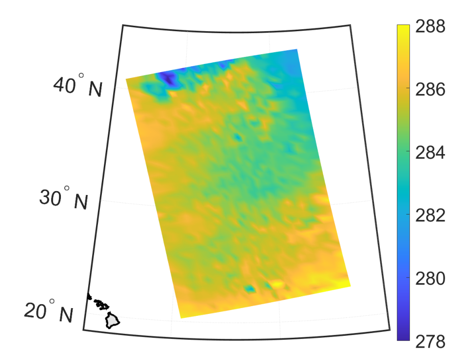
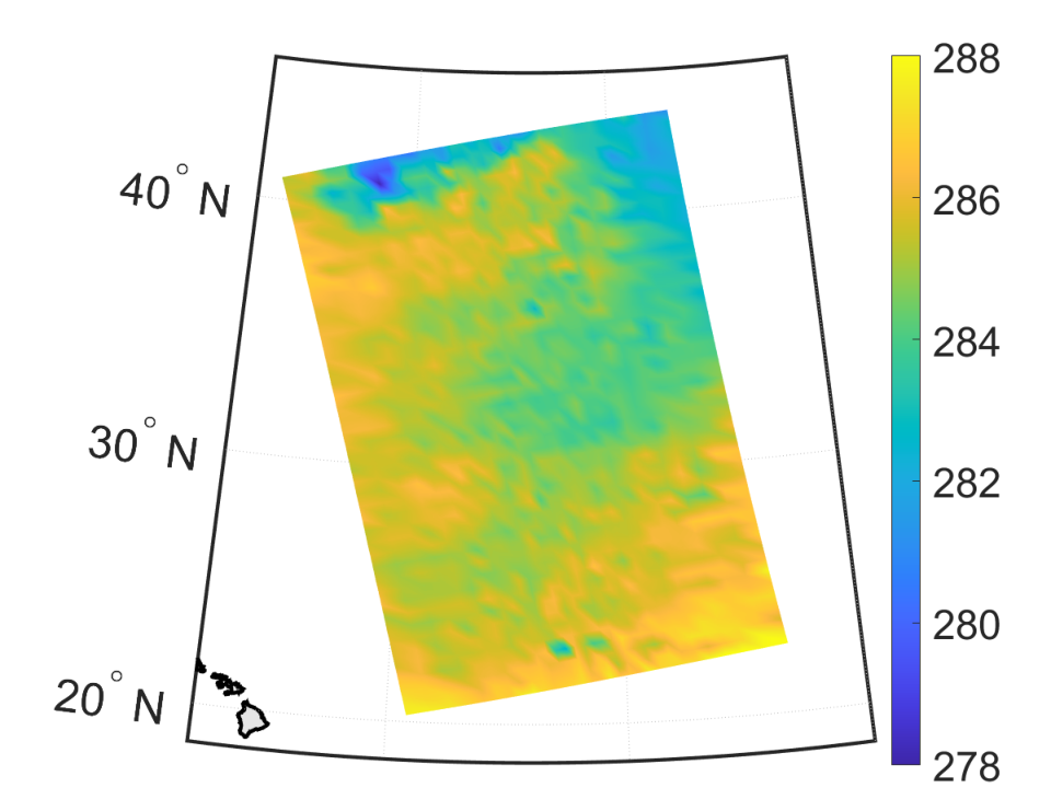
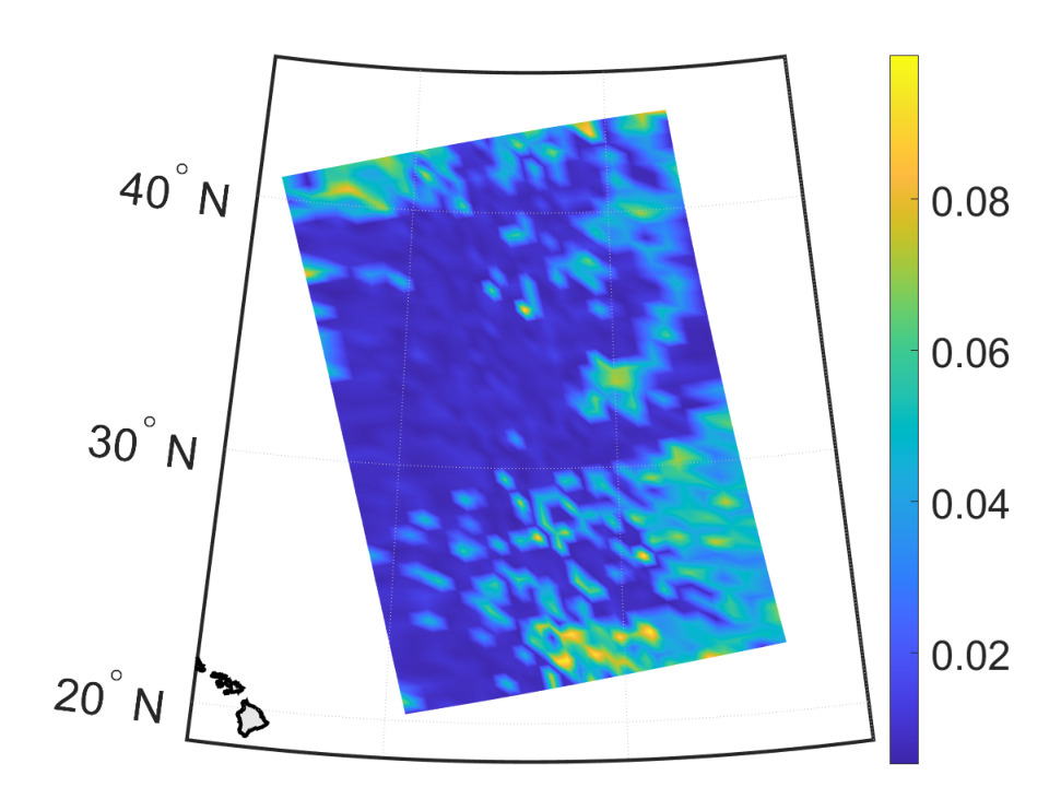
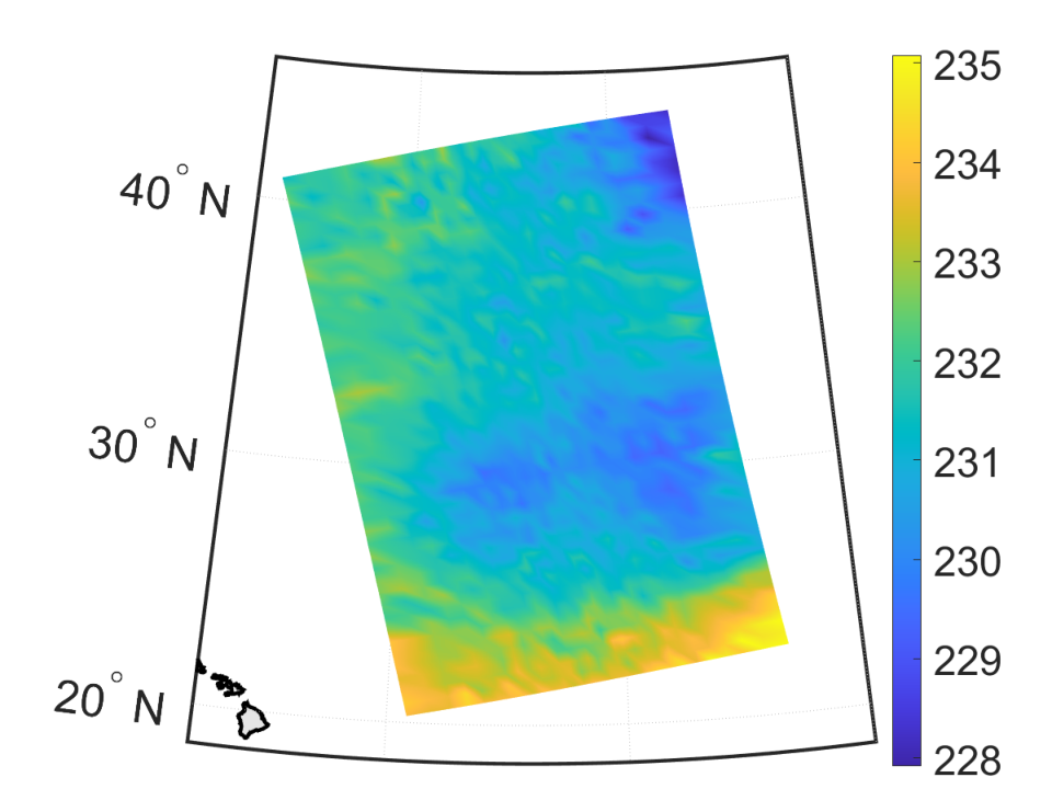
In this paper, we focus on the 3D (longitude, latitude, and pressure level) Level 2 air temperature data product from AIRS, and we choose to focus on a specific granule over the subtropical eastern Pacific Ocean. This region’s weather variability spans multiple cloud regimes that present multiple challenges for remote sensing. Therefore, the region corresponding to this particular granule has been chosen to be the study region in works assessing retrievals from AIRS and other instruments such as the MAGIC validation campaign (Zhou et al. 2015; Kalmus et al. 2015). Figure 1 displays the air temperature in our study region at two different pressure levels, together with their associated QF values. Note that here higher pressure levels means higher pressure values and thus closer to the surface, while lower pressure levels correspond to higher altitudes. The amount of observations with QF value of 1 (i.e., acceptable quality) and 2 (i.e., bad quality) increases as we move from low to high pressure levels. Panels (c) and (d) in Figure 1 show that there are a lot more observations with QF value 1 and 2 at pressure level 90 (pressure level value $\mathchar 29008\mathchar 12349\mathchar 28729\mathchar 28725\mathchar 28728\mathchar 314\mathchar 28725\mathchar 28729\mathchar 28721\mathchar 28721\textrm{ hPa}$) compared to those at pressure level 10 (pressure level value $\mathchar 29008\mathchar 12349\mathchar 28721\mathchar 314\mathchar 28722\mathchar 28729\mathchar 28727\mathchar 28722\textrm{ hPa}$). Meanwhile, it is clear that observations with the same QF values form spatial clusters instead of being distributed uniformly in the region, which is expected as lower quality observations don’t occur randomly but are related to heterogeneous cloud properties at medium or fine spatial scales. Because observations with QF value of 2 are not reliable data, we treat them as missing values in our analysis. For simplicity, we will refer to air temperature data with QF value of 1 as low-fidelity observations and those with QF value of 0 as high-fidelity observations.

Let $\textbf{x}\mathchar 12349\delimiter 67273472\textbf{s}\mathchar 24891\mathchar 29040\delimiter 84054785\mathchar 12850\mathcal{\mathchar 29016}\mathchar 12349\mathcal{\mathchar 29011}\mathchar 8706\mathcal{\mathchar 29008}$ represent the input space with the $\textbf{s}\mathchar 12349\delimiter 67273472\mathchar 29043_{\mathchar 28721}\mathchar 24891\mathchar 29043_{\mathchar 28722}\delimiter 84054785\mathchar 12850\mathcal{\mathchar 29011}\mathchar 12826\mathbb{\mathchar 29010}^{\mathchar 28722}$ denoting the longitude and latitude of the FOR centers and $\mathchar 29040\mathchar 12850\mathcal{\mathchar 29008}\mathchar 12826\mathbb{\mathchar 29010}$ denoting the pressure level values. Let $\left\delimiter 0\delimiter 67273472\mathchar 29050_{\mathchar 29004}\delimiter 67273472\textbf{x}\delimiter 84054785\mathchar 24891\mathchar 29050_{\mathchar 29000}\delimiter 67273472\textbf{x}\delimiter 84054785\delimiter 84054785\mathchar 12346\textbf{x}\mathchar 12850\mathcal{\mathchar 29016}\right\delimiter 0$ represent the observation of low fidelity (QF value 1, subscript $\mathchar 29004$) and high fidelity (QF value 0, subscript $\mathchar 29000$). We assume the data observed at input x is contaminated by additive random noise: $\mathchar 29050_{\mathchar 29004}\delimiter 67273472\textbf{x}\delimiter 84054785\mathchar 12349\mathchar 29049_{\mathchar 29004}\delimiter 67273472\textbf{x}\delimiter 84054785\mathchar 8235\mathchar 28943_{\mathchar 29004}\delimiter 67273472\textbf{x}\delimiter 84054785$ and $\mathchar 29050_{\mathchar 29000}\delimiter 67273472\textbf{x}\delimiter 84054785\mathchar 12349\mathchar 29049_{\mathchar 29000}\delimiter 67273472\textbf{x}\delimiter 84054785\mathchar 8235\mathchar 28943_{\mathchar 29000}\delimiter 67273472\textbf{x}\delimiter 84054785$. Specifically, we model the measurement error of the low fidelity as $\mathchar 28943_{\mathchar 29004}\delimiter 67273472\textbf{x}\delimiter 84054785\mathchar 12824\mathchar 29006\delimiter 67273472\mathchar 28720\mathchar 24891\mathchar 28956_{\mathchar 29004}^{\mathchar 28722}\delimiter 84054785$ and the measurement error of the high fidelity as $\mathchar 28943_{\mathchar 29000}\delimiter 67273472\textbf{x}\delimiter 84054785\mathchar 12824\mathchar 29006\delimiter 67273472\mathchar 28720\mathchar 24891\mathchar 28956_{\mathchar 29000}^{\mathchar 28722}\delimiter 84054785$.

For the latent low- and high-fidelity processes $\mathchar 29049_{\mathchar 29004}\delimiter 67273472\textbf{x}\delimiter 84054785$ and $\mathchar 29049_{\mathchar 29000}\delimiter 67273472\textbf{x}\delimiter 84054785$, we assume that they are linked via the latent variable autoregressive co-kriging model as follows:

where $\mathchar 28954$ represents a constant scalar discrepancy, and $\mathchar 28942_{\mathchar 29000}\delimiter 67273472\textbf{x}\delimiter 84054785$ represents the additive discrepancy between $\mathchar 29049_{\mathchar 29004}\delimiter 67273472\textbf{x}\delimiter 84054785$ and $\mathchar 29049_{\mathchar 29000}\delimiter 67273472\textbf{x}\delimiter 84054785$. Here, $\mathbf{\mathchar 29032}_{\mathchar 29004}\delimiter 67273472\mathchar 8705\delimiter 84054785$ and $\mathbf{\mathchar 29032}_{\mathchar 29000}\delimiter 67273472\mathchar 8705\delimiter 84054785$ are $\mathchar 29040_{\mathchar 29000}$ and $\mathchar 29040_{\mathchar 29004}$ known covariates to describe the mean structure of $\mathchar 29049_{\mathchar 29004}\delimiter 67273472\textbf{x}\delimiter 84054785$ and $\mathchar 28942_{\mathchar 29000}\delimiter 67273472\textbf{x}\delimiter 84054785$, respectively. Utilizing the structure of the observations, we use a product of separate basis functions for the spatial locations and the pressure level values. Suppose, we wish to use $\mathchar 29037_{\mathchar 29004\mathchar 24891\mathchar 29040}$ basis functions to capture the pressure dependence of the lower fidelity mean: $\mathchar 29032_{\mathchar 29004\mathchar 24891\mathchar 29040}\mathchar 12349\{\mathchar 29032_{\mathchar 29004\mathchar 24891\mathchar 29040\mathchar 24891\mathchar 28721}\delimiter 67273472\mathchar 29040\delimiter 84054785\mathchar 24891\dots\mathchar 24891\mathchar 29032_{\mathchar 29004\mathchar 24891\mathchar 29040\mathchar 24891\mathchar 29037_{\mathchar 29004\mathchar 24891\mathchar 29040}}\delimiter 67273472\mathchar 29040\delimiter 84054785\}$. We choose also $\mathchar 29037_{\mathchar 29004\mathchar 24891\mathchar 29043}$ basis functions to capture the spatial dependence of the mean: $\mathchar 29032_{\mathchar 29004\mathchar 24891\bm{\mathchar 29043}}\mathchar 12349\{\mathchar 29032_{\mathchar 29004\mathchar 24891\bm{\mathchar 29043}\mathchar 24891\mathchar 28721}\delimiter 67273472\bm{\mathchar 29043}\delimiter 84054785\mathchar 24891\dots\mathchar 24891\mathchar 29032_{\mathchar 29004\mathchar 24891\bm{\mathchar 29043}\mathchar 24891\mathchar 29037_{\mathchar 29004\mathchar 24891\mathchar 29043}}\delimiter 67273472\bm{\mathchar 29043}\delimiter 84054785\}$. These can be for example the finite element basis of the model or any other suitable functions. This strategy makes possible to separately construct basis functions, in lower dimensions, with the help of the Kronecker product as we explain below. Correspondingly, $\bm{\mathchar 28940}_{\mathchar 29004}$ and $\bm{\mathchar 28940}_{\mathchar 29000}$ are the unknown vectors of coefficient vectors. Finally, we model the latent $\mathchar 29047_{\mathchar 29000}\delimiter 67273472\mathchar 8705\delimiter 84054785$ and $\mathchar 29047_{\mathchar 29004}\delimiter 67273472\mathchar 8705\delimiter 84054785$ as mutually independent Gaussian processes: $\mathchar 29047_{\mathchar 29004}\delimiter 67273472\mathchar 8705\delimiter 84054785\mathchar 12824\mathchar 28999\mathchar 29008\delimiter 67273472\mathchar 28720\mathchar 24891\mathchar 28955_{\mathchar 29004}^{\mathchar 28722}\mathchar 29010_{\mathchar 29004}\delimiter 67273472\mathchar 8705\mathchar 24891\mathchar 8705\mathchar 24635\bm{\mathchar 28946}_{\mathchar 29004}\delimiter 84054785\delimiter 84054785$ where $\mathchar 28955_{\mathchar 29004}^{\mathchar 28722}$ is the variance and $\mathchar 29010_{\mathchar 29004}\delimiter 67273472\mathchar 8705\mathchar 24891\mathchar 8705\mathchar 24635\bm{\mathchar 28946}_{\mathchar 29004}\delimiter 84054785$ is a correlation function with parameters $\bm{\mathchar 28946}_{\mathchar 29004}$ at fidelity level $\mathchar 29004$. Similarly, $\mathchar 29047_{\mathchar 29000}\delimiter 67273472\mathchar 8705\delimiter 84054785\mathchar 12824\mathchar 28999\mathchar 29008\delimiter 67273472\mathchar 28720\mathchar 24891\mathchar 28955_{\mathchar 29000}^{\mathchar 28722}\mathchar 29010_{\mathchar 29000}\delimiter 67273472\mathchar 8705\mathchar 24891\mathchar 8705\mathchar 24891\bm{\mathchar 28946}_{\mathchar 29000}\delimiter 84054785\delimiter 84054785$, but independent of $\mathchar 29047_{\mathchar 29004}\delimiter 67273472\mathchar 8705\delimiter 84054785$.

We define $\bm{\mathchar 28955}^{\bm{\mathchar 28722}}\mathchar 12349\delimiter 67273472\mathchar 28955_{\mathchar 29004}^{\mathchar 28722}\mathchar 24891\mathchar 28955_{\mathchar 29000}^{\mathchar 28722}\delimiter 84054785$, $\bm{\mathchar 28956}^{\bm{\mathchar 28722}}\mathchar 12349\delimiter 67273472\mathchar 28956_{\mathchar 29004}^{\mathchar 28722}\mathchar 24891\mathchar 28956_{\mathchar 29000}^{\mathchar 28722}\delimiter 84054785$, and $\bm{\mathchar 28940}\mathchar 12349\delimiter 67273472\bm{\mathchar 28940}_{\mathchar 29004}\mathchar 24891\bm{\mathchar 28940}_{\mathchar 29000}\delimiter 84054785$, $\bm{\mathchar 28946}\mathchar 12349\delimiter 67273472\bm{\mathchar 28946}_{\mathchar 29004}\mathchar 24891\bm{\mathchar 28946}_{\mathchar 29000}\delimiter 84054785$. A direct Bayesian inference can be computationally costly when the number of the observations is large. The computational complexity of the likelihood is $\mathcal{\mathchar 29007}\delimiter 67273472\mathchar 29038_{\mathchar 29043}^{\mathchar 28723}\mathchar 29038_{\mathchar 29040}^{\mathchar 28723}\delimiter 84054785$ flops and the parameters of the model cannot be expressed in closed form. For more details see Appendix A.

To overcome this computational issue, we assume that the covariance function can be expressed in a multiplicative (separable) form $\mathchar 29010_{\mathchar 29004}\delimiter 67273472\textbf{x}\mathchar 24891\textbf{x}^{\mathchar 560}\mathchar 24635\bm{\mathchar 28946}_{\mathchar 29004}\delimiter 84054785\mathchar 12349\mathchar 29010_{\mathchar 29004\mathchar 24891\mathchar 29043}\delimiter 67273472\textbf{s}\mathchar 24891\textbf{s}^{\mathchar 560}\mathchar 24635\bm{\mathchar 28946}_{\mathchar 29004\mathchar 24891\mathchar 29043}\delimiter 84054785\mathchar 29010_{\mathchar 29004\mathchar 24891\mathchar 29040}\delimiter 67273472\mathchar 29040\mathchar 24891\mathchar 29040^{\mathchar 560}\mathchar 24635\bm{\mathchar 28946}_{\mathchar 29004\mathchar 24891\mathchar 29040}\delimiter 84054785$ and $\mathchar 29010_{\mathchar 29000}\delimiter 67273472\textbf{x}\mathchar 24891\textbf{x}^{\mathchar 560}\mathchar 24635\bm{\mathchar 28946}_{\mathchar 29000}\delimiter 84054785\mathchar 12349\mathchar 29010_{\mathchar 29000\mathchar 24891\mathchar 29043}\delimiter 67273472\textbf{s}\mathchar 24891\textbf{s}^{\mathchar 560}\mathchar 24635\bm{\mathchar 28946}_{\mathchar 29000\mathchar 24891\mathchar 29043}\delimiter 84054785\mathchar 29010_{\mathchar 29000\mathchar 24891\mathchar 29040}\delimiter 67273472\mathchar 29040\mathchar 24891\mathchar 29040^{\mathchar 560}\mathchar 24635\bm{\mathchar 28946}_{\mathchar 29000\mathchar 24891\mathchar 29040}\delimiter 84054785$. This multiplicative (separable) model requires the specification of correlation functions for space and atmospheric pressure for each of the two fidelity levels $\mathchar 29004$ and $\mathchar 29000$. To ensure the well-conditioning of the correlation matrices involved in the calculations, we add nugget effects for the spatial component and for the atmospheric pressure component. In the literature these values are usually fixed based on a cross validation exploration and they are expected to be typically small (of the order of $\mathchar 28721\mathchar 28720^{\mathchar 8704\mathchar 28726}$). In practice, considering these parameters as unknown and estimating them from the data not only improves the stability of the computations but also can lead to better predictive accuracy as shown in our application.

Based on a preliminary study on AIRS data, for both levels of fidelity, we choose a product exponential correlation function:

where $\bm{\mathchar 28946}_{\mathchar 8705\mathchar 24891\mathchar 29043}\mathchar 12349\delimiter 67273472\bm{\mathchar 28958}_{\mathchar 8705\mathchar 24891\mathchar 29043}\mathchar 24891\mathchar 29031_{\mathchar 8705\mathchar 24891\mathchar 29043}^{\mathchar 28722}\delimiter 84054785$, $\bm{\mathchar 28946}_{\mathchar 8705\mathchar 24891\mathchar 29040}\mathchar 12349\delimiter 67273472\mathchar 28958_{\mathchar 8705\mathchar 24891\mathchar 29040}\mathchar 24891\mathchar 29031_{\mathchar 8705\mathchar 24891\mathchar 29040}^{\mathchar 28722}\delimiter 84054785$, $\mathchar 28958_{\mathchar 8705\mathchar 24891\mathchar 28721\mathchar 24891\mathchar 29043}$ controls the spatial dependence strength in longitude, $\mathchar 28958_{\mathchar 8705\mathchar 24891\mathchar 28722\mathchar 24891\mathchar 29043}$ controls the spatial dependence strength in latitude, and $\mathchar 28958_{\mathchar 8705\mathchar 24891\mathchar 29040}$ controls the spatial dependence strength in the pressure level values. Also ${\mathchar 29031}_{\mathchar 8705\mathchar 24891\mathchar 29043}^{\mathchar 28722}$ accounts for the nugget effect in the spatial component and ${\mathchar 29031}_{\mathchar 8705\mathchar 24891\mathchar 29040}^{\mathchar 28722}$ accounts for the nugget effect in the atmospheric pressure component. More intricate covariance functions such as the Matérn family (Cressie 1993; Stein 1999; Banerjee et al. 2014) or non-stationary models (Paciorek and Schervish 2006; Konomi et al. 2014) can also be used within the proposed latent variable co-kriging model.

Despite this flexible and general representation of the separable covariance function, the covariance matrix of the observations or the latent variables cannot be represented as a Kronecker product of separate components. This is simply because none of the input combinations of low and high fidelity data can be represented as a tensor product. The presence of missing data for both quality flags destroys the Kronecker product representation of the covariance matrices and makes the computations impossible in practice.

We make computations and practical implementation possible by constructing an augmented posterior which is based on the imputation of latent variables. The augmented posterior takes advantage of the tensor product of the locations and the pressure level values in a granule. Based on this augmented posterior, we are also able to construct a MCMC procedure with mostly closed form conditional distributions for parameter inference as well as a computationally efficient recursive prediction procedure.

This section conducts a full analysis of the AIRS data set described in Section 2 using the proposed latent variable co-kriging model with separable covariance structure (LVCS). We compare LVCS with two alternatives that ignores the flag values: (a) the latent variable separable Gaussian process (SGP) model; (b) the non-separable additive approximate Gaussian process (AAGP) Ma et al. 2019. For both SGP and AAGP, data with QF values 0 and 1 are combined, and fit with the corresponding model, respectively. Analysis is performed in MATLAB R2020a, on a computer with specifications (intelR i7-3770 3.4GHz Processor, RAM 8.00GB, MS Windows 64bit). In addition, we consider two variations for each of the three models: a) fix the variance of the nugget effects (${\bf\mathchar 29031}_{\mathchar 8705}^{\mathchar 28722}$) within the correlation functions based on a cross validation exploration and b) sample ${\bf\mathchar 29031}_{\mathchar 8705}^{\mathchar 28722}$ within the MCMC procedure as explained in section 4.2.

Each granule has $\mathchar 28721\mathchar 28723\mathchar 28725\mathchar 24891\mathchar 28720\mathchar 28720\mathchar 28720$ estimated temperature values of three different quality flags. Since the vertical pressure levels for atmospheric variables increase in an exponential order, we take a logarithmic transformation of the pressure level values. In each specific FOR, the temperature is taken vertically at $\mathchar 28721\mathchar 28720\mathchar 28720$ distinct pressure level values. Pressure level values with non available (NA) data are removed prior to the analysis. These pressure level values are below the surface pressure and correspond to structurally missing/undefined data due to physical constraints.

We start by testing our proposed model in a granule of August 1 of 2013 within the MAGIC validation campaign Zhou et al. 2015. The last 4 of the distinct pressure levels have only NA data, so we consider only $\mathchar 28729\mathchar 28726$ distinct pressure levels in our analysis. Figure 2a shows the temperature as a function of the log of pressure level values for a collection of FORs with only QF 0 and Figure 2b shows the temperature as a function of pressure level values for FORs with variable quality flags. From these plots as well as Figure 1, one can observe that the QF 1 and 2 data are more common in higher vertical pressure levels (closer to the sea surface) within the vertical profile.

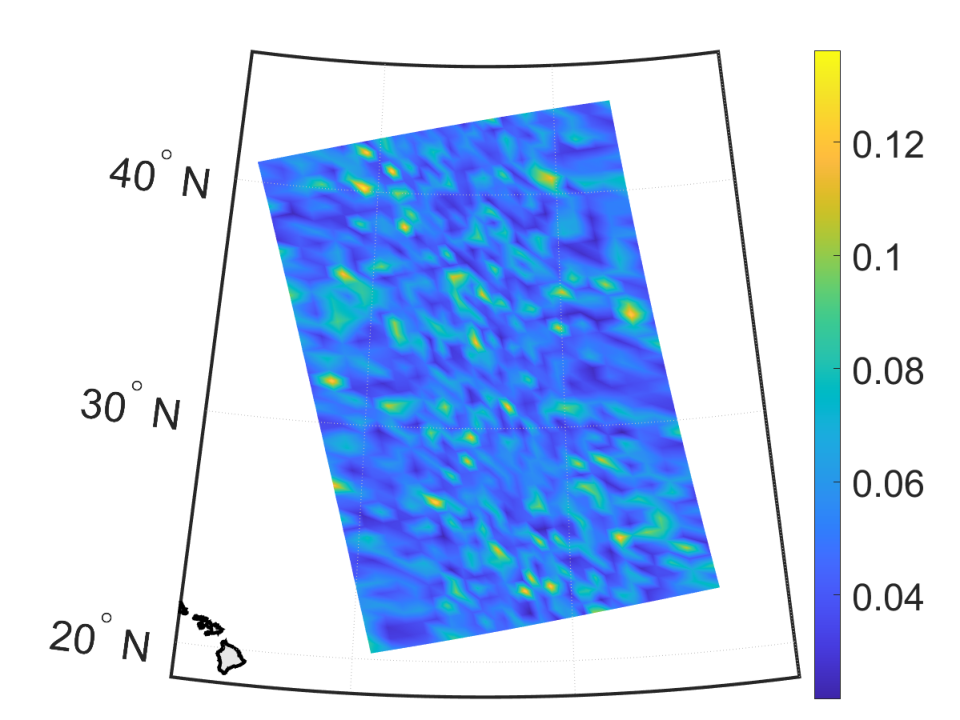
To simulate a realistic missing data (i.e., with QF 2) scenario, we randomly select testing data in a block of input. Since missing observations are more common in higher vertical atmospheric pressure values (close to the sea surface), we only consider vertical atmospheric pressure values higher than $\mathchar 28721\mathchar 28721\mathchar 28724\mathchar 314\mathchar 28720\mathchar 28720\mathchar 28727\mathchar 28720$ hPa (pressure level greater than $\mathchar 28724\mathchar 28727$). Evaluation of predictive performance is based on mean squared prediction errors (MSPE), coverage probability of the $\mathchar 28729\mathchar 28725\%$ equal tail credible interval (CVG($\mathchar 28729\mathchar 28725\%$)), average length of the $\mathchar 28729\mathchar 28725\%$ equal tail credible interval (ALCI($\mathchar 28729\mathchar 28725\%$)), and continuous rank probability score (CRPS)(Gneiting and Raftery 2007).

Based on the relationship of the log pressure values with the data Figure 2, we chose polynomial basis functions of degree three for the log pressure level. Since we do not observe a spatial structure of the mean of temperature given a pressure level, we chose a constant mean for the spatial basis. The basis functions of the complete data are created based on the Kronecker product of these two bases. Based on an empirical study between three different covariance functions; the square exponential, exponential, and the $\mathchar 28725\delimiter 68408078\mathchar 28722$ Matérn; we chose the exponential covariance function. For all the tested days and models, the exponential covariance function gave the best prediction performance.

We apply the same specifications for all three models, the proposed LVCS, the separable model, and the AAGP. To speed up computations in the AAGP we specify a grid of knots: $\mathchar 28721\mathchar 28725$ knots for pressure level, $\mathchar 28728$ knots for longitude and $\mathchar 28726$ for latitude. In total, we use $\mathchar 28727\mathchar 28722\mathchar 28720$ knots for the predictive process part and the same specification for the separable part. For the Bayesian inference of the three models on the unknown parameters $\bm{\mathchar 28940}_{\mathchar 28721}\mathchar 24891\bm{\mathchar 28940}_{\mathchar 28722}$, we assigned independent Normal prior distributions with zero mean and large variances. We used inverse Gamma priors for the spatial and noise variances $\mathchar 28955_{\mathchar 29004}^{\mathchar 28722}\mathchar 24891\mathchar 28955_{\mathchar 29000}^{\mathchar 28722}\mathchar 24891\mathchar 28956_{\mathchar 29004}^{\mathchar 28722}\mathchar 24891\mathchar 28956_{\mathchar 29000}^{\mathchar 28722}$ as $\mathchar 29001\mathchar 28999\delimiter 67273472\mathchar 28722\mathchar 24891\mathchar 28721\delimiter 84054785$. The range correlation parameters in space are assigned a uniform prior $\mathchar 29013\delimiter 67273472\mathchar 28720\mathchar 24891\mathchar 28721\mathchar 28720\mathchar 28720\delimiter 84054785$ and the range correlation parameters in logarithmic pressure level values a uniform prior $\mathchar 29013\delimiter 67273472\mathchar 28720\mathchar 24891\mathchar 28722\mathchar 28720\delimiter 84054785$ . For all three models, we ran the MCMC sampler as described in Section $\mathchar 28723$ with $\mathchar 28722\mathchar 28725\mathchar 24891\mathchar 28720\mathchar 28720\mathchar 28720$ iterations where the first $\mathchar 28725\mathchar 24891\mathchar 28720\mathchar 28720\mathchar 28720$ iterations were discarded as burn-in. For all the parameters of the three models the MCMC converges within the first $\mathchar 28722\mathchar 24891\mathchar 28720\mathchar 28720\mathchar 28720$ iterations. The convergence of the MCMC sampler for each parameter was assessed from their associated trace plots.

Table 1 shows the results with the prediction performances for each model when we assume an unknown nugget effect ($\mathchar 29031_{\mathchar 8705}^{\mathchar 28722}$) within the correlation functions as described in section 3 and when we fix it to $\mathchar 28721\mathchar 28720^{\mathchar 8704\mathchar 28726}$. Based on the MSPE and CRPS the proposed LVCS kriging gives better prediction results than the separable kriging and the AAGP for both fixed or random nugget effects cases. Making the nugget effect random improves the predictability for all models. The proposed LVCS has smaller MSPE and CRPS than both the separable kriging and the AAGP kriging. Specifically, the MSPE of the proposed model is less than half of both AAGP and separable model. The LVCS has nominal coverage probability close to $\mathchar 28720\mathchar 314\mathchar 28729\mathchar 28725$ and short interval length for the 95% credible interval. The separable model and the AAGP kriging have very similar MSPE which indicates that AIRS data have a separable covariance structure. The computational time for the AAGP is almost $\mathchar 28721\mathchar 28720$ times slower. It is worth pointing out that we can improve the computational time of AAGP by decreasing the number of predictive process knots. However, this may result in missing a potential non-separable small scale variation.

To better demonstrate the prediction benefit of accounting for the quality flag into our model, we plot the predicted temperature values against held-out temperature values for pressure level values between $\mathchar 28727\mathchar 28725\mathchar 28720$ hPa and $\mathchar 28728\mathchar 28725\mathchar 28720$ hPa using: (a) Figure 3a the model which ignores the quality flag of the data and (b) Figure 3b the proposed LVCS model which accounts for different quality flags. From these scatter plots it is clear that accounting for the different quality of the retrievals improves predictions. Specifically the predicted temperature values of the proposed LVCS scattered in a narrower interval around the $\mathchar 28724\mathchar 28725$ degree straight red line. The fact that the predicted values when ignoring the fidelity level are still scattered around the $\mathchar 28724\mathchar 28725$ degree straight red line indicates that the flag one observations may be unbiased estimates of the temperature with bigger variance.

We are able to reconstruct the 3D observations with the high fidelity (quality flag 0). Given the MCMC sample from fitting the model, the reconstruction based on the quality flag 0 data is automatic and does not require additional computational burden. Figure 4a shows the observed temperature values of mixed quality flags at vertical pressure level $\mathchar 28728\mathchar 28722\mathchar 28727$ hPa (pressure level 89). Figure 4b shows the corresponding quality flag values of the data based on the locations. Figure 4c shows the quality flag $\mathchar 28720$ predicted mean values of the temperature at vertical pressure level $\mathchar 28728\mathchar 28722\mathchar 28727$ hPa using the proposed recursive prediction procedure. The two images have a lot of similarities with more significant differences when the quality flag values are equal to 2 (Figure 4b). Also the proposed procedure can take into account the parameter uncertainty as well as the nugget effects. Figure 4d shows the predictive variance of the predicted values. There is a clear association of the the variance with the quality flag values and the spatial proximity as they are shown in Figure 4b.

Within the boundaries of a granule, we can also use the proposed procedure to predict the air temperature values at a unmeasured vertical pressure level different from those 100 levels in AIRS data products, i.e, interpolating vertically and horizontally. Given the MCMC values obtained in fitting of the model, we can find the predictive distribution for any location and vertical pressure value. With $\mathchar 28722\mathchar 28720\mathchar 24891\mathchar 28720\mathchar 28720\mathchar 28720$ posterior samples of model parameters, the total computing time to make prediction for a vertical pressure level at the specified granule locations is about 145.5 seconds based on Matlab 2020 on a laptop with specifications described above. For example Figure 5a shows the predicted temperature and Figure 5b shows the associated standard deviation for unmeasured vertical pressure level value $\mathchar 28722\mathchar 28726\mathchar 28725$ hPa which corresponds to pressure level between $\mathchar 28726\mathchar 28720$ and $\mathchar 28726\mathchar 28721$.

Within the study region of the subtropical eastern Pacific Ocean, we repeat the proposed model and inference for five different granules on different days in August 2013. Two different models are considered: a) the SGP which ignores the quality flag and b) the proposed LVCS which accounts for the quality flag. Because the AAGP gives similar results to the SGP and it is computationally more expensive, we discard it from this analysis. This is also a strong evidence of the separable covariance structure between coordinates and atmospheric pressure for the AIRS observation. We follow the same computational strategy as explained above where the MCMC is run in a sequence for both models. Table 2 shows that the MSPE applying the LVCS is consistently almost half to the MSPE if we ignore the different flag quality. These results strengthen our modeling approach to account for different quality flags when we analyse AIRS temperature data sets.

In this paper, we propose a latent variable co-kriging model with separable Gaussian processes (LVCS) to analyze 3D AIRS air temperature data with different quality flags from NASA’s AIRS instrument. We propose an MCMC procedure with an imputation mechanism which takes advantage of the 3D input structure to facilitate efficient computation. By applying our method to the AIRS data, we demonstrate that incorporating the quality-flag information into statistical modeling and data analysis can provide substantial inferential benefits. Unlike other methods for NASA’s AIRS mission in the literature (Tian et al. 2020; Waliser et al. 2020, e.g.,), we allow for different fidelity and missing data. Our methodology provides a coherent framework for the combined use of remote sensing retrievals with variable quality in both the horizontal and vertical directions. This capability can bolster the utility of observations from AIRS and next-generation infrared sounder instruments, particularly in challenging observing conditions such as the subtropical ocean regions illustrated in this work.

Our LVCS model can be generalized for larger spatial data sets over multiple granules. For example, we may apply a computationally efficient method such as low-dimensional conditional approximation (Datta et al. 2016; Katzfuss and Guinness 2021, e.g.,) for both horizontal and vertical components in the separable covariance function. It is also possible to extend our method for multi-fidelity spatio-temporal remote sensing data by adding the temporal dependence and considering 4D data (longitude, latitude, vertical pressure level and time). Extending the LVCS modeling framework for multivariate multi-fidelity data could also prove to be fruitful.

The current LVCS model assumes a linear relationship between low- and high-fidelity levels. One direction in future research is to extend this work by borrowing the idea of deep Gaussian process in Perdikaris et al. 2017 and Ming et al. 2021 so that we can incorporate nonlinear dependence structure into the model. In addition, the LVCS modeling framework can be applied in observing system uncertainty experiments (Hobbs et al. 2017; Turmon and Braverman 2019; Braverman et al. 2021; Ma et al. 2021), in particular when surrogates with different fidelity levels and computational efficiency are used to perform forward uncertainty propagation and inverse calibration for remote sensing data products.

The research of Konomi and Kang was partially supported by National Science Foundation grant NSF DMS-2053668. Kang was also partially supported by Simons Foundation’s Collaboration Award (#317298 and #712755), and the Taft Research Center at the University of Cincinnati.Part of this work was performed at the Jet Propulsion Laboratory, California Institute of Technology, under contract with NASA. Support was provided by the Atmospheric Infrared Sounder (AIRS) mission. The authors thank Amy Braverman and Hai Nguyen for valuable discussions during the course of this work.

References

• Banerjee (2017) Banerjee, S. (2017), “High-Dimensional Bayesian Geostatistics,” Bayesian Analysis, 12, 583 – 614, URL https://doi.org/10.1214/17-BA1056R.
• Banerjee et al. (2014) Banerjee, S., Carlin, B. P., and Gelfand, A. E. (2014), Hierarchical Modeling and Analysis for Spatial Data, New York: Chapman and Hall/CRC, second edition.
• Banerjee et al. (2008) Banerjee, S., Gelfand, A. E., Finley, A. O., and Sang, H. (2008), “Gaussian predictive process models for large spatial data sets,” Journal of the Royal Statistical Society: Series B (Statistical Methodology), 70, 825–848.
• Behrangi et al. (2016) Behrangi, A., Fetzer, E. J., and Granger, S. L. (2016), “Early detection of drought onset using near surface temperature and humidity observed from space,” International Journal of Remote Sensing, 37, 3911–3923.
• Bilionis et al. (2013) Bilionis, I., Zabaras, N., Konomi, B. A., and Lin, G. (2013), “Multi-output separable Gaussian process: Towards an efficient, fully Bayesian paradigm for uncertainty quantification,” Journal of Computational Physics, 241, 212–239.
• Braverman et al. (2021) Braverman, A., Hobbs, J., Teixeira, J., and Gunson, M. (2021), “Post hoc Uncertainty Quantification for Remote Sensing Observing Systems,” SIAM/ASA Journal on Uncertainty Quantification, 9, 1064–1093, URL https://doi.org/10.1137/19M1304283.
• Cheng et al. (2021) Cheng, S., Konomi, B. A., Matthews, J. L., Karagiannis, G., and Kang, E. L. (2021), “Hierarchical Bayesian Nearest Neighbor Co-Kriging Gaussian Process Models; An Application to Intersatellite Calibration,” Spatial Statistics, 44, 100516.
• Cressie (1993) Cressie, N. (1993), Statistics for Spatial Data, New York: John Wiley & Sons, revised edition.
• Cressie and Johannesson (2008) Cressie, N. and Johannesson, G. (2008), “Fixed rank kriging for very large spatial data sets,” Journal of the Royal Statistical Society: Series B (Statistical Methodology), 70, 209–226.
• Datta et al. (2016) Datta, A., Banerjee, S., Finley, A. O., and Gelfand, A. E. (2016), “Hierarchical nearest-neighbor Gaussian process models for large geostatistical datasets,” Journal of the American Statistical Association, 111, 800–812.
• Gelfand and Smith (1990) Gelfand, A. E. and Smith, A. F. M. (1990), “Sampling-Based Approaches to Calculating Marginal Densities,” Journal of the American Statistical Association, 85, 398–409.
• Genton (2007) Genton, M. G. (2007), “Separable approximations of space-time covariance matrices,” Environmetrics, 18, 681–695.
• Gneiting and Raftery (2007) Gneiting, T. and Raftery, A. E. (2007), “Strictly Proper Scoring Rules, Prediction, and Estimation,” Journal of the American Statistical Association, 102, 359–378.
• Gramacy (2020) Gramacy, R. B. (2020), Surrogates: Gaussian Process Modeling, Design and Optimization for the Applied Sciences, Boca Raton, Florida: Chapman Hall/CRC. http://bobby.gramacy.com/surrogates/.
• Gramacy and Apley (2015) Gramacy, R. B. and Apley, D. W. (2015), “Local Gaussian Process Approximation for Large Computer Experiments,” Journal of Computational and Graphical Statistics, 24, 561–578.
• Guillas et al. (2018) Guillas, S., Sarri, A., Day, S. J., Liu, X., and Dias, F. (2018), “Functional emulation of high resolution tsunami modelling over Cascadia,” The Annals of Applied Statistics, 12, 2023 – 2053, URL https://doi.org/10.1214/18-AOAS1142.
• Hastings (1970) Hastings, W. K. (1970), “Monte Carlo sampling methods using Markov chains and their applications,” Biometrika, 57, 97–109.
• Heaton et al. (2019) Heaton, M. J., Datta, A., Finley, A., Furrer, R., Guhaniyogi, R., Gerber, F., Gramacy, R. B., Hammerling, D., Katzfuss, M., Lindgren, F., Nychka, D., Sun, F., and Zammit-Mangion, A. (2019), “A Case Study Competition Among Methods for Analyzing Large Spatial Data,” Journal of Agricultural, Biological and Environmental Statistics, 24, 398–425.
• Hobbs et al. (2017) Hobbs, J., Braverman, A., Cressie, N., Granat, R., and Gunson, M. (2017), “Simulation-Based Uncertainty Quantification for Estimating Atmospheric CO2 from Satellite Data,” SIAM/ASA Journal on Uncertainty Quantification, 5, 956–985.
• Kahn et al. (2014) Kahn, B. H., Irion, F. W., Dang, V. T., Manning, E. M., Nasiri, S. L., Naud, C. M., Blaisdell, J. M., Schreier, M. M., Yue, Q., Bowman, K. W., Fetzer, E. J., Hulley, G. C., Liou, K. N., Lubin, D., Ou, S. C., Susskind, J., Takano, Y., Tian, B., and Worden, J. R. (2014), “The Atmospheric Infrared Sounder version 6 cloud products,” Atmospheric Chemistry and Physics, 14, 399–426, URL https://acp.copernicus.org/articles/14/399/2014/.
• Kalmus et al. (2015) Kalmus, P., Wong, S., and Teixeira, J. (2015), “The Pacific Subtropical Cloud Transition: A MAGIC Assessment of AIRS and ECMWF Thermodynamic Structure,” IEEE Geoscience and Remote Sensing Letters, 12, 1586–1590.
• Katzfuss (2017) Katzfuss, M. (2017), “A multi-resolution approximation for massive spatial datasets,” Journal of the American Statistical Association, 112, 201–214.
• Katzfuss and Guinness (2021) Katzfuss, M. and Guinness, J. (2021), “A general framework for Vecchia approximations of Gaussian processes,” Statistical Science, 36, 124–141.
• Kennedy and O’Hagan (2000) Kennedy, M. C. and O’Hagan, A. (2000), “Predicting the output from a complex computer code when fast approximations are available,” Biometrika, 87, 1–13.
• Konomi and Karagiannis (2021) Konomi, B. A. and Karagiannis, G. (2021), “Bayesian Analysis of Multifidelity Computer Models With Local Features and Nonnested Experimental Designs: Application to the WRF Model,” Technometrics, 63, 510–522.
• Konomi et al. (2014) Konomi, B. A., Sang, H., and Mallick, B. K. (2014), “Adaptive Bayesian Nonstationary Modeling for Large Spatial Datasets Using Covariance Approximations,” Journal of Computational and Graphical Statistics, 23, 802–829.
• Lindgren et al. (2011) Lindgren, F., Rue, H., and Lindström, J. (2011), “An explicit link between Gaussian fields and Gaussian Markov random fields: the stochastic partial differential equation approach,” Journal of the Royal Statistical Society: Series B (Statistical Methodology), 73, 423–498.
• Lu and Zhang (2019) Lu, Y. and Zhang, F. (2019), “Toward Ensemble Assimilation of Hyperspectral Satellite Observations with Data Compression and Dimension Reduction Using Principal Component Analysis,” Monthly Weather Review, 147, 3505––3518.
• Ma and Kang (2020a) Ma, P. and Kang, E. L. (2020a), “A Fused Gaussian Process Model for Very Large Spatial Data,” Journal of Computational and Graphical Statistics, 29, 479–489.
• Ma and Kang (2020b) — (2020b), “Spatio-Temporal data fusion for massive sea surface temperature data from MODIS and AMSR-E instruments,” Environmetrics, 31, e2594. E2594 env.2594.
• Ma et al. (2019) Ma, P., Konomi, B. A., and Kang, E. L. (2019), “An additive approximate Gaussian process model for large spatio-temporal data,” Environmetrics, 30, e2569.
• Ma et al. (2021) Ma, P., Mondal, A., Konomi, B. A., Hobbs, J., Song, J. J., and Kang, E. L. (2021), “Computer Model Emulation with High-Dimensional Functional Output in Large-Scale Observing System Uncertainty Experiments,” Technometrics, 0, 1–15.
• Ming et al. (2021) Ming, D., Williamson, D., and Guillas, S. (2021), “Deep Gaussian Process Emulation using Stochastic Imputation,” .
• Mueller (1993) Mueller, P. (1993), “Alternatives to the Gibbs sampling scheme,” Technical report, Institute Statistics and Decision Sciences, Duke University.
• Nychka et al. (2015) Nychka, D., Bandyopadhyay, S., Hammerling, D., Lindgren, F., and Sain, S. (2015), “A multiresolution Gaussian process model for the analysis of large spatial datasets,” Journal of Computational and Graphical Statistics, 24, 579–599.
• Paciorek and Schervish (2006) Paciorek, C. and Schervish, M. (2006), “Spatial modelling using a new class of nonstationary covariance functions,” Environmetrics, 17, 483–506.
• Perdikaris et al. (2017) Perdikaris, P., Raissi, M., Damianou, A., Lawrence, N., and Karniadakis, G. E. (2017), “Nonlinear information fusion algorithms for data-efficient multi-fidelity modelling,” Proceedings of the Royal Society A: Mathematical, Physical and Engineering Sciences, 473, 20160751.
• Peruzzi et al. (2020) Peruzzi, M., Banerjee, S., and Finley, A. O. (2020), “Highly Scalable Bayesian Geostatistical Modeling via Meshed Gaussian Processes on Partitioned Domains,” Journal of the American Statistical Association, 0, 1–14.
• Prata and Lynch (2019) Prata, F. and Lynch, M. (2019), “Passive Earth Observations of Volcanic Clouds in the Atmosphere,” Atmosphere, 10, 199.
• Qian and Wu (2008) Qian, P. Z. and Wu, C. J. (2008), “Bayesian hierarchical modeling for integrating low-accuracy and high-accuracy experiments,” Technometrics, 50, 192–204.
• Roberts et al. (2004) Roberts, G. O., Rosenthal, J. S., et al. (2004), “General state space Markov chains and MCMC algorithms,” Probability surveys, 1, 20–71.
• Rougier (2008) Rougier, J. (2008), “Efficient Emulators for Multivariate Deterministic Functions,” Journal of Computational and Graphical Statistics, 17, 827–843.
• Sang and Huang (2012) Sang, H. and Huang, J. Z. (2012), “A full scale approximation of covariance functions for large spatial data sets,” Journal of the Royal Statistical Society: Series B (Statistical Methodology), 74, 111–132.
• Stein (1999) Stein, M. L. (1999), Interpolation of Spatial Data: Some Theory for Kriging. 2nd edition, New York: Springer.
• Stein et al. (2004) Stein, M. L., Chi, Z., and Welty, L. J. (2004), “Approximating likelihoods for large spatial data sets,” Journal of the Royal Statistical Society: Series B (Statistical Methodology), 66, 275–296.
• Susskind et al. (2003) Susskind, J., Barnet, C. D., and Blaisdell, J. M. (2003), “Retrieval of atmospheric and surface parameters from AIRS/AMSU/HSB data in the presence of clouds,” IEEE Transactions on Geoscience and Remote Sensing, 41, 390–409.
• Thrastarson et al. (2021) Thrastarson, H. T., Manning, E., Kahn, B., Fetzer, E. J., Yue, Q., Wong, S., Kalmus, P., Payne, V., Olsen, E. T., Wilson, R. C., Blaisdell, J., Iredell, L., Susskind, J., Warner, J., and Cady-Pereira, K. (2021), “AIRS/AMSU/HSB Version 7 Level 2 Product User Guide,” URL URL:https://docserver.gesdisc.eosdis.nasa.gov/public/project/AIRS/V7_L2_Product_User_Guide.pdf.
• Tian et al. (2020) Tian, B., Manning, E., Roman, J., Thrastarson, H., Fetzer, E., and Monarrez, R. (2020), “AIRS Version 7 Level 3 Product User Guide,” URL URL:https://docserver.gesdisc.eosdis.nasa.gov/public/project/AIRS/V7_L3_Product_User_Guide.pdf.
• Turmon and Braverman (2019) Turmon, M. and Braverman, A. (2019), “Uncertainty quantification for JPL retrievals,” Technical report, Pasadena, CA: Jet Propulsion Laboratory, National Aeronautics and Space Administration, 2019. Http://hdl.handle.net/2014/45978.
• Vecchia (1988) Vecchia, A. V. (1988), “Estimation and model identification for continuous spatial processes,” Journal of the Royal Statistical Society: Series B (Methodological), 50, 297–312.
• Waliser et al. (2020) Waliser, D., Gleckler, P. J., Ferraro, R., Taylor, K. E., Ames, S., Biard, J., Bosilovich, M. G., Brown, O., Chepfer, H., Cinquini, L., Durack, P. J., Eyring, V., Mathieu, P.-P., Lee, T., Pinnock, S., Potter, G. L., Rixen, M., Saunders, R., Schulz, J., Thépaut, J.-N., and Tuma, M. (2020), “Observations for Model Intercomparison Project (Obs4MIPs): status for CMIP6,” Geoscientific Model Development, 13, 2945–2958.
• Zhou et al. (2015) Zhou, X., Kollias, P., and Lewis, E. R. (2015), “Clouds, Precipitation, and Marine Boundary Layer Structure during the MAGIC Field Campaign,” Journal of Climate, 28, 2420 – 2442.
• Zhu et al. (2015) Zhu, Y., Kang, E. L., Bo, Y., Tang, Q., Cheng, J., and He, Y. (2015), “A Robust Fixed Rank Kriging Method for Improving the Spatial Completeness and Accuracy of Satellite SST Products,” IEEE Transactions on Geoscience and Remote Sensing, 53, 5021–5035.
Refer to caption
(a)
(b)
(c)
(d)
Figure 1: Top: AIRS retrieved temperature (units are Kelvin) on two different pressure levels, a) pressure level 10 (P=1.2​9​7​2​ hPa\mathchar 29008\mathchar 12349\mathchar 28721\mathchar 314\mathchar 28722\mathchar 28729\mathchar 28727\mathchar 28722\textrm{ hPa}) and b) pressure level 90 (P=9​5​8.5​9​1​1​ hPa\mathchar 29008\mathchar 12349\mathchar 28729\mathchar 28725\mathchar 28728\mathchar 314\mathchar 28725\mathchar 28729\mathchar 28721\mathchar 28721\textrm{ hPa}). Bottom: Retrieved temperature quality flag on two different pressure levels, c) pressure level 10 (P=1.2​9​7​2​ hPa\mathchar 29008\mathchar 12349\mathchar 28721\mathchar 314\mathchar 28722\mathchar 28729\mathchar 28727\mathchar 28722\textrm{ hPa}) and d) pressure level 90 (P=9​5​8.5​9​1​1​ hPa\mathchar 29008\mathchar 12349\mathchar 28729\mathchar 28725\mathchar 28728\mathchar 314\mathchar 28725\mathchar 28729\mathchar 28721\mathchar 28721\textrm{ hPa})
Figure 2: AIRS retrieved temperature (units are Kelvin) as a function of log pressure levels: a) Quality flag 0 only b) Quality flag 1 (Red), and 2 (Blue).
Figure 3: Scatter plot of predicted values against held-out testing data for the last three pressure levels values using two different models: a) Separable model, and b) the proposed latent variable co-kriging model with separable covariance structure (LVCS)
Figure 4: a) AIRS air temperature data (units in Kelvin) b) the corresponding quality flag values c) Predicted means of the temperature with quality flag value 0, d) Prediction standard error
Figure 5: a) Predicted means of the temperature (units are Kelvin) at 2​6​5\mathchar 28722\mathchar 28726\mathchar 28725 hPa with quality flag value 0, b) Prediction standard error.
Model Nugget MSPE CRSP CVG 95% ALCI 95% Time (hours)
SGP Fixed 0.2714 0.3011 84.9% 1.8113 3.973
Random 0.2503 0.2974 89.2% 1.9213 5.977
AAGP Fixed 0.2783 0.3361 91.7% 2.089 65.402
Random 0.2482 0.3361 92.3% 2.139 96.419
LVCS Fixed 0.1341 0.2323 92.9% 1.58 7.801
Random 0.1081 0.2270 96.1% 1.63 10.432