Quantum Machine Learning for Material Synthesis and Hardware Security (Invited Paper)DOI: XXXXXXX.XXXXXXXConference: International Conference on Computer-Aided Design 2022; Oct 29 – Nov 03, 2022; San Diego, CAPrice: 15.00ISBN: 978-1-4503-XXXX-X/18/06CCS: Computing methodologies Neural networksCCS: Computer systems organization Quantum computing
Abstract.
Using quantum computing, this paper addresses two scientifically-pressing and day to day-relevant problems, namely, chemical retrosynthesis which is an important step in drug/material discovery and security of semiconductor supply chain. We show that Quantum Long Short-Term Memory (QLSTM) is a viable tool for retrosynthesis. We achieve 65% training accuracy with QLSTM whereas classical LSTM can achieve 100%. However, in testing we achieve 80% accuracy with the QLSTM while classical LSTM peaks at only 70% accuracy! We also demonstrate an application of Quantum Neural Network (QNN) in the hardware security domain, specifically in Hardware Trojan (HT) detection using a set of power and area Trojan features. The QNN model achieves detection accuracy as high as 97.27%.
Keywords:
Quantum computing, quantum machine learning, chemical retrosynthesis, drug discovery, machine learning, Trojan, hardware Trojan, hardware security, LSTM, QLSTM, QNN, quantum neural network1. Introduction
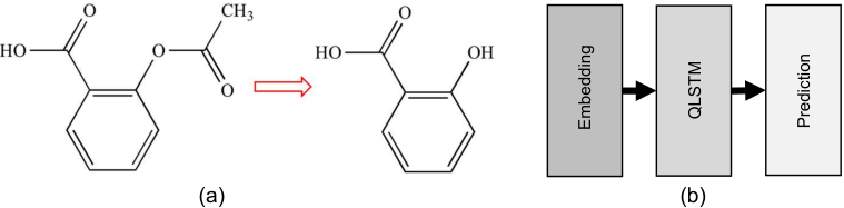
Problem 1, chemical retrosynthesis: Chemical retrosynthesis attempts to provide reactants that can be combined, using a chemical reaction, to synthesize a desired molecule. This process defines fields such as agriculture, medical treatment, material discovery, and countless others. Fig. 1a exemplifies the retrosynthesis process, where the chemical on the left can be formed by the chemical on the right in combination of a chemical reaction. Performing retrosynthesis in the lab using trial-and-error takes years, and possibly cost billions of dollars, to resolve just for a single chemical. This leads to an immense amount of interest in machine learning (ML)-based solutions. Previous work have been able to generate promising results, but suffer from limitations. For example, expert defined rules for retrosynthesis (Socorro et al. 2005) relies on human’s incomplete knowledge of retrosynthesis and doesn’t scale well as more rules are being defined. To overcome limitations of domain knowledge, models have been created that do not require prior knowledge (Liu et al. 2017; Wang et al. 2021). These solutions ignore the certainty of domain knowledge, require excessive training time, and still poses scalability issues, making it hard to solve retrosynthesis of large molecules (Dai et al. 2019). Another common issue is a dependence on a predefined library of solutions rather than coming up with unique chemical results (Gómez-Bombarelli et al. 2016). The efforts to resolve these issues run into the difficulty of finding chemically viable solutions, long training times, etc. (Gómez-Bombarelli et al. 2018; Rappoport et al. 2014). Chemical retrosynthesis could benefit from more capability than what modern machines offer, prompting us to search for solutions in new hardware domains.
The promise of exponential growth in computational space has led to the idea of Quantum Neural Networks (QNN) (Kak 1995) and more recently the Quantum Long Short-Term Memory (QLSTM) (Chen et al. 2022). Unfortunately, Quantum Machine Learning (QML) efforts have fallen short of their desired exponential gain in speed (Ciliberto et al. 2018). However, they still offer the ability to represent an exponentially growing amount of information with only a linear growth in hardware size.
We evaluate the performance of QLSTM (a quantum-classical hybrid approach) and compare it to the performance of LSTM in its ability to make retrosynthetic predictions using the USPTO-50k dataset (Lowe 2012). We also introduce two unique approaches to simplify the retrosynthesis process by identifying a specific substring within the reactants that are used to produce the given reaction.
Problem 2, security of semiconductor supply chain: In recent years, the hardware supply chain has been flooded with low-quality counterfeit Integrated Circuits (IC). The ICs suffer from a variety of threats/vulnerabilities such as, manufacturing defects, malicious circuitry, reverse engineering, etc. Hardware Trojans (HTs) tamper the circuitry posing a threat to IC trustworthiness since it could severely disrupt system functionality/security. Prior work has exploited classical ML to automate and provide a more reliable solution to the HT detection problem. In (Hasegawa et al. 2017), 51 Trojan features are proposed to describe Trojan nets from gate-level netlists, use a random forest classifier to extract the best 11 Trojan features, and train a classifier to perform the classification task. The work in (Yasaei et al. 2021) utilizes a graph data structure for hardware representation and generates Data Flow Graphs (DFG) from RTL codes. Then Graph Neural Network (GNN) is used to extract features from the DFG and detect the presence of HT. A possible application of QML in classifying PCB defects (which can severely hinder system performance if undetected) from images is proposed in (Kundu and Ghosh 2022). However, detection of HT has not been addressed yet.
To solve the above challenge, we evaluate the performance of a QNN model in detecting HTs from a small number of features. We also compare the results of our QNN with a few traditional ML classifiers and neural networks. Specifically, we use a Trojan feature dataset consisting of 50 features (of area and power), reduce feature size to 2 features using a dimensionality reduction algorithm, T-distributed Stochastic Neighbor Embedding (t-SNE), and then train a 2-qubit QNN using those features to evaluate the performance of the quantum model.
2. Background
2.1. Material Discovery
Material discovery extensively employs USPTO-50K dataset (Lowe 2012) which consists of 40,000 training, 5,000 validation, and 5,000 testing SMILES formatted chemical examples. SMILES is originally created as a way to use characters to represent chemical chains (Weininger 1988). The letters represent various elements within the chain where the first letter of an element can be uppercase, denoting that the element is non-aromatic, or lowercase, denoting that the element is aromatic. If an element requires a second letter it will be lowercase, regardless of the casing of the first letter. Numbers are used within the chain to represent the opening and closing of a ring. Finally, parenthesis are used to denote branches from a chain, whereas periods are used to denote the start of a new chemical.
| (1) |
The input from USPTO-50K consists of two parts, the first part is the reaction type that causes the reaction whereas the second part of the string is the reaction. The reaction type consists of 10 different possible values, ranging from 1-10. The output consists of possible input reactants that can be used in combination with the reaction type to create the final reaction. Exemplifying the SMILES format in Eq. 1, the initial six characters, (), represent the reaction type that causes the target molecule given certain reactant(s). Following the reaction type, we have the chemical , which breaks down into three unique pieces. makes the initial chain, while forms a separate chain, which is denoted by the parentheses. Finally, we end with a third smaller chain, . Next is the use of and , in the uppercase we note there is only a single non-aromatic carbon used, while the rest of the carbon in the chain is aromatic. Finally, we consider the use of numbers. Within the separate chain marked by the parentheses, we note the smallest ring formed, , this is the third ring in the set, which is why it is marked by two different 3s. Since the creation of the USPTO-50K, it has frequently been used as an experimental testing ground for chemical retrosynthesis (Shi et al. 2020; Dai et al. 2019; Wang et al. 2021). We note that due to the nature of this difficult problem and unlike familiar benchmarks in other domains, the accuracy of much of this work rarely reaches higher than 50% while predicting the proper reactant for a given input. Although 50% is typically associated with random guessing, in this domain the accuracy relies on the exact match of reactant(s) to the given reaction. Given each reaction can have one or two reactants, and the majority of these reactants are unique to their reaction, it is easy to see 50% accuracy is far higher than random guess. We summarize the results from previous work in Table 1.
| Model Type | Resulting Top 1 Accuracy |
|---|---|
| G2Gs (Shi et al. 2020) | 48.9% |
| GLN (Dai et al. 2019) | 52.5% |
| RetroPrime (Wang et al. 2021) | 51.4% |
| Augmented Transformer (Tetko et al. 2020) | 53.5% |
2.2. Qubits
The qubit is the basis for all quantum computing, similar to its classical counterpart, the bit. But, there is a significant advantage of the qubit. Unlike the classical bit a qubit stores a mix of two states together, which is called superposition. For a single qubit, the states and are called our basis states. It is from these basis states that almost all quantum computation stems from.
2.3. Quantum Gates
Quantum gates are operations that are performed on qubits, similar to classical gates. These quantum gates are used to change the state of the qubits on which the operation is being performed. They typically are represented in the form of unitary matrices which operate on some initial qubit state. The most common quantum gates are the Hadamard (H), Bit flip (X) and Rotation gate (RX, RY, RZ) which are all single qubit gates. While the Controlled Not (CNOT) is a two-qubit gate. These gates allow us to perform almost all of our basic encodings of data in the quantum state, allowing for meaningful computation of quantum information.
2.4. LSTM
LSTM is an adaptation of the original Recurrent Neural Network (RNN) structure which is designed to keep temporal storage of information. This allows the neural network to maintain previous states of information. However, there is no guarantee as to what information is held and for how long it will remain, causing saturation issues. To get around these issues the LSTM allows for the neural network to decide when to add/remove pieces of information, helping mitigate context saturation issues.

2.5. QLSTM
There have been many attempts in the quantum computing domain to create trainable networks (Cong et al. 2019; Kak 1995) to solve classification problems. However, selective memory has not been available. QLSTM addresses this challenge and offers the same advantage as classical LSTMs, i.e., the ability to intentionally form a contextual understanding of previous input. This approach is near identical to the classical LSTM. The divergence of the two occurs when the network, instead of taking the information directly from the hidden layer and the input, takes the information and pass it to a Variational Quantum Circuit (VQC) where we can perform a data entanglement of the values. We then perform a measurement on the entangled information and proceed to process it in the same prediction structure as the classical LSTM. Fig. 1b displays the basic overall architecture of the network: embedding, QLSTM and prediction. Embedding is preferred to a bag of words model as it reduces potentially large sparse vectors to smaller dense vectors that require less memory. Fig. 2 shows the structure of the QLSTM. Starting with our representation choices, we use the round edge boxes to represent the external values fed into the QLSTM, each varying in size. For the size is dependant on the embedding layer whereas for and the size is defined by the hidden dimension size. We use the sharp-cornered boxes to represent layers of a network, and circles to represent pointwise functions. For the wires, as displayed in the key, we use the wire merging to represent concatenation and wire splitting to represent a copy of the wire. We also use to represent the sigmoid activation function, defined by Eq. 2, and tanh is the arctan activation function, defined by Eq. 3.
| (2) |
| (3) |
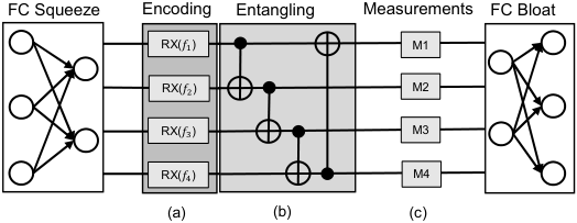
Working through the QLSTM starting with the bottom left, we have which represents the input to the QLSTM structure. The input is concatenated with the previous hidden layer information, which is represented as . This combination is fed into four different VQCs; each of them are defined by a modified version of the basic entangler circuit from Fig. 3.
The modified basic entangler includes a trainable fully connected layer that squeezes the dimensional space of the information down to the circuit size of the VQC. After each VQC a quantum measurement of the expectation for each wire is fed to the trainable fully connected bloating layer. The bloating layer, increases the size from the quantum circuit back to the required dimensional space of the classical network. This is then processed using classical LSTM approaches. Hence, this is a quantum-classical hybrid approach. The first sigmoid activation is known as the forget gate which is used to decide whether to update the context to include the new input. After the sigmoid, the result is multiplied onto . The second sigmoid, and the activations are known as the input gate which is used to write the new input into the context. The result of the sigmoid and tanh activations are multiplied to either be added to , or to ensure the input is not added to . The last sigmoid activation is known as the output gate where the actual prediction is performed. This output is also used to update the hidden layer .
2.6. QNN
QNN is a promising QML model that has received a lot of attention in recent years. A traditional QNN is made up of a data encoding circuit, a Parametric Quantum Circuit (PQC), and measurement operations. The data encoder transforms classical data into a quantum state. The PQC transforms the quantum state using a chosen ansatz. Measurements determine the output state. The PQC parameters are tuned during the training phase to produce the desired measurement results. We can train QNN models to perform traditional ML tasks such as classification, regression, distribution generation, etc. by selecting appropriate cost functions.
Fig. 4 shows the architecture of the 2-qubit QNN we used for training. It consists of the (a) Encoding, (b) PQC and (c) Measurement blocks. Several encoding techniques have been explored, e.g., amplitude encoding, basis encoding, NEQR (Zhang et al. 2013). We employ angle encoding where we pass classical features () as angles of quantum rotations gates () to transform them to quantum state. Similar to angle encoding, there are a number of PQC ansatz (Sim et al. 2019) to choose from but almost all of the PQCs consists of two main gate types: single qubit gates which are used to perform design space exploration, and two qubit gates which are used to entangle the qubits. The latter forms a correlation between the qubits based on the input feature values.
In the QNN, we use the 2-qubit Controlled-RZ () gate to entangle the qubits and rotation gates along X and Z axes () for transformation/exploration. The PQC/QNN is analogous to a classical neural network where we adjust the weights () to reduce the loss value while we adjust the tunable parameters () to generate the desired output in QNN. Finally, to measure the qubit state the most widely used measurement technique is Pauli’s measurement along any of the X, Y, or Z axes. In our QNN model we used Pauli-Z measurement (). A measurement in the Pauli Z basis means projecting the state onto one of the states or (the eigenstates of Pauli Z matrix).

3. Proposed Methodology
3.1. Chemical Retrosynthesis
Previous works on retrosynthesis have addressed the problem from many different ways such as, using graph, transformer or some other approach. Prior to transformers, LSTMs were the preferred approach to neural networks that required a memory (Vaswani et al. 2017). However, LSTMs don’t work as well as transformers. Therefore, we propose two unique approaches to simplify the problem of retrosynthesis namely, (a) we restrict the reactions by selecting just a single reaction type, , in an attempt to simplify the retrosynthesis process. This subset is reduced from 12,000 to just 9 samples to reduce training time, and emulate the proof of concept proposed by Di Sipio (Di Sipio et al. 2022) (b) We revert back to including all reaction types and change our output from a prediction of the reactants to a prediction of a chemical chain within the reactant. For this we select acetic acid and acetone as the common chemical chains and reduce the input reactions to only options that produce the selected chemical chains. This subset is reduced from 2,100 samples down to 200, which is then splitted 90:10 between training-validation set so there are 180 training samples and 20 validation samples. We then introduce these approaches to the QLSTM to show the potential of quantum computing in chemical retrosynthesis. In order to implement the encoding and the required layers for both LSTM and QLSTM, as well as the sigmoid activation and arctan activation function for the QLSTM, we use Pytorch (Paszke et al. 2019). The quantum circuits are trained using pennylane (Bergholm et al. 2018).
3.2. Hardware Trojan Detection
Here we consider a 50-feature dataset (Liakos et al. 2019), which was originally created from Trojan free (TF) and Trojan infected (TI) circuits/ benchmarks available in Trust-Hub (Shakya et al. 2017), a public benchmark library. This original feature set containing area and power characteristics of the TI/TF circuits has been created using an industrial circuit design tool (DC compiler Synopsys). However, the feature set had a total of 900 samples among which very few samples of TF circuits were present compared to TI ones with a TF:TI ratio of 1:40. Thus, a reproduction technique (e.g., by repeating the TF circuit features to match the number of TI ones for each circuit/benchmark category) has been used to balance out the ratio between TF and TI samples. The resultant feature set that we use for our evaluation purposes contains 3026 samples and 50 features. We tested our models on both the original and reproduced/augmented dataset.
Since it is not ideal to directly train a QNN using a dataset containing such larger number of features, we compress the information down to a handful of meaningful features. In the noisy quantum computing era, with access to a hardware with low qubits, it is critical to reduce dataset dimension to train QNNs efficiently. Although we can run quantum simulations in classical computers, they incur a very high computational cost. As a result, we use a non-linear dimensionality reduction technique, specifically T-distributed Stochastic Neighbor Embedding (t-SNE) (Van der Maaten and Hinton 2008), to reduce the feature size from 50 to 2 features for training our QNN. Although t-SNE is widely used as a visualization technique as it helps clearly visualize multiple class high dimensional data in 2D/3D space, it can also be used as a dimension reduction technique. This is true since it generates low number of high variance features which can help train networks/classifiers effectively. Lastly, we normalize the features of this reduced dimension dataset before training our QNN (as shown in Fig. 4). More specifically, we use the "max" normalization technique provided by the sklearn library (Pedregosa et al. 2011), which divides each feature value with the max feature value of that specific row (). The need to normalize the features before training comes from the fact that, during the encoding step, as we are passing the features as rotation angle values of quantum gates, it is possible that feature values of different classes differ by a multiple of and thus end up being treated as features of the same class by our QNN (as ).
4. Results
4.1. Experimental Setups
Since we adopt unique approaches to perform chemical retrosynthesis our results cannot be directly compared to other state-of-the-art work. For a fair comparison we create a classical LSTM in the same form as the QLSTM. The QLSTM depends on a 4 qubit VQC structure, while relatively small, the 4 qubit structure allows for a more manageable run time. Both the QLSTM and the LSTM use a small embedding dimension size of 8, and a small hidden dimension size of 6. The small embedding dimension is used for two reasons: first, it allows for enough memory for the second approach where we are predicting a reactant sub-string, and still uses a smaller vector than a bag of words would use for the proof of concept. The second reason is that when the concatenation of and occurs, it doesn’t require a large fully connected layer squeeze/bloat to match the size of the VQC structure. The hidden dimension size is heuristically selected, using values less than the embedding dimension, in expectation to keep the fully connected layer size requirement low. For the concatenation it is performed such that appends to . Table 2 contains a summation of parameters. All performance results are reported from execution on an Intel Xeon W-2125 CPU running at 4 GHz, with 16 GB of RAM.
| Parameter | VQC size | |||
|---|---|---|---|---|
| Value | 8x1 dim | 6x1 dim | 6x1 dim | 4 qubits |
For the second problem, the train-test split of 90:10 is used. We further used 10% of the training data for validating the model Therefore, training, testing and validation employs 2452, 302 and 272 samples, respectively. We trained the QNN for 10 epochs with the following parameters; Loss function: Sparse Categorical Cross Entropy (Abadi et al. 2015), Optimizer: Adagrad (Duchi et al. 2011) , Learning rate: 0.4, and Batch size: 32. All simulations were performed using Pennylane’s (Bergholm et al. 2018) default.qubit device on a computer equipped with a 12th Gen Intel(R) Core(TM) i7-12700H and 16GB RAM.
4.2. Single Reaction Type Retrosynthesis
Before beginning the single reaction type retrosynthesis some preprocessing of the original data is required. For clarity, an example string is provided for each step. To begin we take the initial input strings, as seen below.
We note here that the use of multiple lines are meaningless, they are just inserted for readability purposes. For simplicity and legibility, we use superscript numbers to represent a repeating series of a character. This format will be followed for the continuation of the work:
As part of our method, we then compress by removing all of the individual spacing, as this space does not carry any special meaning in the context of SMILES format:
We then ensure the reaction type is the first reaction type, matching the . After this we strip off the reaction type as it is no longer helpful:
After finishing the input string, we take the output string for processing. Here we match the input string to the output string to find the corresponding output:
After we find the matching output string, we simply compress the string by removing the spaces:
Once the trimming of the input and output is done, we perform a word encoding for both the input and the output to have a numerical representation of the SMILES strings for use in LSTM. The word encoding requires two unique lists, one for reactions and another for reactants. Each list consists of unique chemicals, where each chemical is assigned it’s numerical value based on it’s index within the list it belongs to. After completing the preprocessing we train the LSTM and QLSTM models. The promising results in Fig. 5(a) show that the quantum approach, while unable to match the results of classical approach, is able converge to an accuracy of 65% and a loss of 0.1.
4.3. Chemical Chain Prediction
We perform similar preprocessing of the original data as explained with an example string below. We take the initial output strings from the input file:
We then remove all of the individual spacing:
We then ensure the reaction contains the acetic acid chain, or acetone . After this we dispose of the reactant and simply use the label of the chain the string contains, for example: acetic.
After we finish the output string, we take the input string and match it to the output string to find the corresponding input:
After we find the matching input string, we remove the spaces, and the reaction type:
Once the trimming of the input and output is done, we perform our encoding and we train the LSTM and QLSTM models. The results in Fig. 5(b) show that the classical loss never reaches a point of convergence, where the quantum loss also doesn’t reach convergence nor does it reach the same level as the classical. These results hold true for accuracy, where the classical domain reaches 65% and the quantum domain reaches 55%. While there is a small gap in performance, we see that given the task of identifying a common substring within the predicted reactants, quantum is able to nearly match classical performance during training. Validation is ran once every 5 epochs during training and here, there is a flip of performance. The results in Fig. 6 show that the classical loss starts to increase after just 25 training epochs, whereas the quantum loss is steadily decreasing for the entirety of the training. As for the accuracy, the classical accuracy reaches a high of 70% and steadily decreases to 40%. For the quantum domain the accuracy starts at 50%, while steadily increasing all the way to 80%, outperforming the classical model by 40% at the end of the model training.
4.4. Trojan Detection
Coming to the second problem we study, Fig. 7 shows the accuracy and loss comparison of our QNN with a simple classical neural network on the augmented dataset with the following neuron configuration; 2-64-256-64-2 per the five layers from input to output. We trained our classical NN for 10 epochs [Optimizer: Adam (Kingma and Ba 2014), Loss_Fn: Sparse Categorical Cross Entropy (Abadi et al. 2015) and Learning rate: 0.01]. The maximum training accuracy achieved by our QNN and classical NN was 91.06% and 98.03% respectively.
| Model | Training Acc. | Testing Acc. |
|---|---|---|
| Perceptron | 73.72% | 72.61% |
| GaussianNB | 74.92% | 76.73% |
| LogisticRegression | 75.04% | 73.76% |
| QuantumNN | 91.06% | 90.04% |
| SVM | 96.49% | 96.04% |
| ClassicalNN | 98.03% | 98.35% |
We also trained some of the linear/non-linear ML classifiers with the augmented dataset of features and compared the results of the same with our QNN model. From Table 3 we can see that QNN performs better than few of the linear/non-linear models (Perceptron/GaussianNB) but falls behind SVM and classical neural network. The results clearly show that the classes are not linearly separable because linear classifiers like Perceptron and Logistic Regression perform poorly, as shown in Table 3.
Without employing the reproducing technique, we also trained our QNN and traditional NN model with the original feature set ( samples). We only modified one parameter before training the models; the learning rate, which we lowered to 0.01 and 0.001 for QNN and classicalNN, respectively. In this case, the QNN model is found to be more effective at detecting HTs, with a classification accuracy of up to 97.27%. The QNN model performed identical to classicalNN, which produced an accuracy of 97.09%. As a result, we can conclude that QNN models can potentially perform similar to classical neural networks in some cases.
It should be noted that the goal of this work is not to demonstrate superior classification accuracy over classical counterparts, but rather to show a proof-of-concept application of QML in hardware security domain. We posit that further optimization of the feature count, qubits, layers, epochs and/or lower the learning rate could achieve higher detection accuracy.
5. Conclusion and Future Work
We have shown that QLSTM is a viable solution to solve chemical retrosynthesis problem, even with just 4 qubits. While QLSTM didn’t train as well as its classical counterpart, it is able to reach a reasonable accuracy and loss metrics for the proof of concept. For example, quantum achieves 65% accuracy and classical achieves 100%. It again is able to reach a reasonable accuracy e.g., 55% for quantum and 65% for classical while attempting to predict substrings. However these gaps are misleading since quantum is able to reach an accuracy or 80% whereas classical peaks at an accuracy of 70% during testing of the substring prediction! We also demonstrated a QNN application in hardware security domain, specifically Trojan detection from a set of area and power features. A very simple 2-qubit QNN with demonstrated () accuracy is able to outperform some linear/non-linear classifiers which show in terms of detection accuracy. In the future, the performance of the model can be improved by using a Quantum RAM (QRAM) to load the data and/or using a Quantum Graph Neural Network (QGNN) instead of QNN.
Acknowledgements.
The work is supported in parts by NSF (CNS-1722557, CNS-2129675, CCF-2210963, CCF-1718474, OIA-2040667, DGE-1723687, DGE-1821766 and DGE-2113839) and seed grants from Penn State ICDS and Huck Institute of the Life Sciences.References
- (1)
- Abadi et al. (2015) Martín Abadi et al. 2015. TensorFlow: Large-Scale Machine Learning on Heterogeneous Systems. https://www.tensorflow.org/ Software available from tensorflow.org.
- Bergholm et al. (2018) Ville Bergholm et al. 2018. PennyLane: Automatic differentiation of hybrid quantum-classical computations. arXiv e-prints, Article arXiv:1811.04968 (Nov. 2018), arXiv:1811.04968 pages. arXiv:1811.04968 [quant-ph]
- Bergholm et al. (2018) Ville Bergholm, Josh Izaac, Maria Schuld, Christian Gogolin, M Sohaib Alam, Shahnawaz Ahmed, Juan Miguel Arrazola, Carsten Blank, Alain Delgado, Soran Jahangiri, et al. 2018. Pennylane: Automatic differentiation of hybrid quantum-classical computations. arXiv preprint arXiv:1811.04968 (2018).
- Chen et al. (2022) Samuel Yen-Chi Chen, Shinjae Yoo, and Yao-Lung L Fang. 2022. Quantum long short-term memory. In ICASSP 2022-2022 IEEE International Conference on Acoustics, Speech and Signal Processing (ICASSP). IEEE, 8622–8626.
- Ciliberto et al. (2018) Carlo Ciliberto et al. 2018. Quantum machine learning: a classical perspective. Proceedings of the Royal Society A: Mathematical, Physical and Engineering Sciences 474, 2209 (2018), 20170551.
- Cong et al. (2019) Iris Cong, Soonwon Choi, and Mikhail D Lukin. 2019. Quantum convolutional neural networks. Nature Physics 15, 12 (2019), 1273–1278.
- Dai et al. (2019) Hanjun Dai, Chengtao Li, Connor Coley, Bo Dai, and Le Song. 2019. Retrosynthesis prediction with conditional graph logic network. Advances in Neural Information Processing Systems 32 (2019).
- Di Sipio et al. (2022) Riccardo Di Sipio, Jia-Hong Huang, Samuel Yen-Chi Chen, Stefano Mangini, and Marcel Worring. 2022. The dawn of quantum natural language processing. In ICASSP 2022-2022 IEEE International Conference on Acoustics, Speech and Signal Processing (ICASSP). IEEE, 8612–8616.
- Duchi et al. (2011) John Duchi, Elad Hazan, and Yoram Singer. 2011. Adaptive Subgradient Methods for Online Learning and Stochastic Optimization. J. Mach. Learn. Res. 12, null (jul 2011), 2121–2159.
- Gómez-Bombarelli et al. (2016) Rafael Gómez-Bombarelli et al. 2016. Design of efficient molecular organic light-emitting diodes by a high-throughput virtual screening and experimental approach. Nature materials 15, 10 (2016), 1120–1127.
- Gómez-Bombarelli et al. (2018) Rafael Gómez-Bombarelli et al. 2018. Automatic chemical design using a data-driven continuous representation of molecules. ACS central science 4, 2 (2018), 268–276.
- Hasegawa et al. (2017) Kento Hasegawa, Masao Yanagisawa, and Nozomu Togawa. 2017. Trojan-feature extraction at gate-level netlists and its application to hardware-Trojan detection using random forest classifier. In 2017 IEEE International Symposium on Circuits and Systems (ISCAS). IEEE, 1–4.
- Kak (1995) Subhash C Kak. 1995. Quantum neural computing. Advances in imaging and electron physics 94 (1995), 259–313.
- Kingma and Ba (2014) Diederik P. Kingma and Jimmy Ba. 2014. Adam: A Method for Stochastic Optimization. (2014). https://doi.org/10.48550/ARXIV.1412.6980
- Kundu and Ghosh (2022) Satwik Kundu and Swaroop Ghosh. 2022. Security Aspects of Quantum Machine Learning: Opportunities, Threats and Defenses. In Proceedings of the Great Lakes Symposium on VLSI 2022. 463–468.
- Liakos et al. (2019) Konstantinos G Liakos, Georgios K Georgakilas, Serafeim Moustakidis, Patrik Karlsson, and Fotis C Plessas. 2019. Machine learning for hardware trojan detection: a review. In 2019 Panhellenic Conference on Electronics & Telecommunications (PACET). IEEE, 1–6.
- Liu et al. (2017) Bowen Liu, Bharath Ramsundar, Prasad Kawthekar, Jade Shi, Joseph Gomes, Quang Luu Nguyen, Stephen Ho, Jack Sloane, Paul Wender, and Vijay Pande. 2017. Retrosynthetic reaction prediction using neural sequence-to-sequence models. ACS central science 3, 10 (2017), 1103–1113.
- Lowe (2012) Daniel Mark Lowe. 2012. Extraction of chemical structures and reactions from the literature. Ph.D. Dissertation. University of Cambridge.
- Paszke et al. (2019) Adam Paszke et al. 2019. PyTorch: An Imperative Style, High-Performance Deep Learning Library. Curran Associates, Inc., 8024–8035. http://papers.neurips.cc/paper/9015-pytorch-an-imperative-style-high-performance-deep-learning-library.pdf
- Pedregosa et al. (2011) F. Pedregosa et al. 2011. Scikit-learn: Machine Learning in Python. Journal of Machine Learning Research 12 (2011), 2825–2830.
- Rappoport et al. (2014) Dmitrij Rappoport, Cooper J Galvin, Dmitry Yu Zubarev, and Alán Aspuru-Guzik. 2014. Complex chemical reaction networks from heuristics-aided quantum chemistry. Journal of chemical theory and computation 10, 3 (2014), 897–907.
- Shakya et al. (2017) Bicky Shakya, Tony He, Hassan Salmani, Domenic Forte, Swarup Bhunia, and Mark Tehranipoor. 2017. Benchmarking of hardware trojans and maliciously affected circuits. Journal of Hardware and Systems Security 1, 1 (2017), 85–102.
- Shi et al. (2020) Chence Shi, Minkai Xu, Hongyu Guo, Ming Zhang, and Jian Tang. 2020. A graph to graphs framework for retrosynthesis prediction. In International Conference on Machine Learning. PMLR, 8818–8827.
- Sim et al. (2019) Sukin Sim, Peter D Johnson, and Alán Aspuru-Guzik. 2019. Expressibility and entangling capability of parameterized quantum circuits for hybrid quantum-classical algorithms. Advanced Quantum Technologies 2, 12 (2019), 1900070.
- Socorro et al. (2005) Ingrid M Socorro, Keith Taylor, and Jonathan M Goodman. 2005. ROBIA: a reaction prediction program. Organic letters 7, 16 (2005), 3541–3544.
- Tetko et al. (2020) Igor V Tetko, Pavel Karpov, Ruud Van Deursen, and Guillaume Godin. 2020. State-of-the-art augmented NLP transformer models for direct and single-step retrosynthesis. Nature communications 11, 1 (2020), 1–11.
- Van der Maaten and Hinton (2008) Laurens Van der Maaten and Geoffrey Hinton. 2008. Visualizing data using t-SNE. Journal of machine learning research 9, 11 (2008).
- Vaswani et al. (2017) Ashish Vaswani, Noam Shazeer, Niki Parmar, Jakob Uszkoreit, Llion Jones, Aidan N Gomez, Łukasz Kaiser, and Illia Polosukhin. 2017. Attention is all you need. Advances in neural information processing systems 30 (2017).
- Wang et al. (2021) Xiaorui Wang, Yuquan Li, et al. 2021. RetroPrime: A Diverse, plausible and Transformer-based method for Single-Step retrosynthesis predictions. Chemical Engineering Journal 420 (2021), 129845.
- Weininger (1988) David Weininger. 1988. SMILES, a chemical language and information system. 1. Introduction to methodology and encoding rules. Journal of chemical information and computer sciences 28, 1 (1988), 31–36.
- Yasaei et al. (2021) Rozhin Yasaei, Shih-Yuan Yu, and Mohammad Abdullah Al Faruque. 2021. Gnn4tj: Graph neural networks for hardware trojan detection at register transfer level. In 2021 Design, Automation & Test in Europe Conference & Exhibition (DATE). IEEE, 1504–1509.
- Zhang et al. (2013) Yi Zhang, Kai Lu, Yinghui Gao, and Mo Wang. 2013. NEQR: a novel enhanced quantum representation of digital images. Quantum information processing 12, 8 (2013), 2833–2860.