Metric Residual Networks for Sample Efficient
Goal-Conditioned Reinforcement Learning
Abstract
Goal-conditioned reinforcement learning (GCRL) has a wide range of potential real-world applications, including manipulation and navigation problems in robotics. Especially in such robotics tasks, sample efficiency is of the utmost importance for GCRL since, by default, the agent is only rewarded when it reaches its goal. While several methods have been proposed to improve the sample efficiency of GCRL, one relatively under-studied approach is the design of neural architectures to support sample efficiency. In this work, we introduce a novel neural architecture for GCRL that achieves significantly better sample efficiency than the commonly-used monolithic network architecture. The key insight is that the optimal action-value function must satisfy the triangle inequality in a specific sense. Furthermore, we introduce the metric residual network (MRN) that deliberately decomposes the action-value function into the negated summation of a metric plus a residual asymmetric component. MRN provably approximates any optimal action-value function , thus making it a fitting neural architecture for GCRL. We conduct comprehensive experiments across 12 standard benchmark environments in GCRL. The empirical results demonstrate that MRN uniformly outperforms other state-of-the-art GCRL neural architectures in terms of sample efficiency. The code is publicly available at https://github.com/Cranial-XIX/metric-residual-network.
1 Introduction
Goal-conditioned reinforcement learning (GCRL) refers to the problem in which an agent learns to solve a set of tasks indicated by different “goals” via trial and error. In contrast to the standard reinforcement learning (RL) setting, in which the per-step reward the agent receives can be an arbitrary fixed scalar function, the reward function in GCRL is usually an indicator function identifying whether the agent has achieved the goal but with a varying goal. As a result, GCRL enables the learning of a whole family of tasks with relatively little human effort toward reward design and thus has many potential real-world applications. For instance, robot manipulation tasks like picking and placing an object in a target location can be viewed as a GCRL problem where the underlying task family is parameterized by the target goal location. Similarly, robot navigation can be viewed as a GCRL problem where the goal can be any navigation destination.
Although GCRL has a straightforward reward formulation, it inherits the challenges associated with sparse reward learning: unlike in the dense reward setting, the reward signal is only informative when the agent reaches the goal. Therefore, sample efficiency is a major challenge in GCRL, meaning that the agent typically needs a large number of interactions with the environment to make meaningful learning progress. To address this problem, an active line of research focuses on designing novel learning algorithms that efficiently use the data. One popular approach is hindsight experience replay (HER) (Andrychowicz et al. 2017), which relabels the agent’s trajectories as if they were aiming to reach the state that they in fact reached, thus rendering every trajectory an example of a successful goal achievement.
One relatively under-explored direction is the design of better neural architectures for GCRL. For actor-critic-like methods, prior work has proposed decomposing the critic function (a.k.a the action-value function , see Sec. 2.1) into a bilinear network, e.g., either (Schaul et al. 2015) or (Hong, Yang, and Agrawal 2022), where and are separate neural modules. The principle behind these designs is to inject useful inductive bias into the architecture. Although empirically found to be effective, it remains unclear why such a decomposition works and whether it can be improved upon.
In this work, we argue that one fundamental inductive bias is that under the sparse reward setting, the negated optimal action-value (e.g., ) must satisfy the triangle inequality in a specific sense. While there exists prior work on neural architectures that respect the triangle inequality (Pitis et al. 2020), we make the following novel contributions:
- •
We are the first to show that the discounted in the standard GCRL setting (See Sec. 2.1), when the goal is a deterministic onto mapping from the state, satisfies the triangle inequality.
- •
Motivated by the first point, we introduce the metric residual network (MRN) that deliberately decomposes the negative action-value function (e.g., ) into the sum of a metric and an asymmetric residual component, which provably approximates any quasipseudometric.11 1 defines a quasipseudometric on if 1) and 2) .
- •
With a comprehensive experiment on 12 standard GCRL benchmark environments, MRN consistently performs better than a range of common prior designs. We hypothesize that MRN’s metric component speeds up learning, and the asymmetric residual component makes the approximation accurate.

2 Preliminaries
In this section, we first introduce the formal definition of the GCRL problem. Then we review the off-policy actor-critic algorithm DDPG and the hindsight experience replay (HER) method with goal relabeling for GCRL. DDPG+HER serves as the substrate algorithm within which we compare different neural architecture designs.
2.1 Goal-conditioned Reinforcement Learning
The goal-conditioned reinforcement learning problem can be formulated as a goal-conditioned Markov Decision Process, which is an 8-tuple . Here, , , and are the state, action, and goal spaces of the agent. is the transition dynamics. is the reward function. is the discount factor. and are the initial state and target goal distributions. Concretely, at the start of each episode, an initial state and a goal are sampled. The agent starts at , and at each time step , it chooses action from a policy , e.g., . It then receives a reward and transitions to the next state . The overall objective of the infinite-horizon GCRL problems is to maximize the following:
| (1) |
where the reward is often defined as22 2 There are two conventional setups: either the agent receives a reward of when reaching the goal and otherwise, or it receives reward until it reaches the goal. In this work, without further specification, we assume the latter setting.
| (2) |
Here is an onto mapping from the product space of the state and action to the goal space. Note that does not terminate when the goal is reached; the agent receives a reward every time it returns to the goal (or remains there). In practice, usually . For example, if the goal is for an autonomous car to reach any given velocity, then would naturally comprise the velocity component of the agent’s full state space . For technical reasons in Sec. 3.1, we also include in deciding whether the goal is reached.33 3 When is determined by checking whether , as opposed to whether , it is a deterministic function involving no randomness from the transition dynamics .
2.2 Off-Policy Actor-Critic
Actor-critic methods like Deep Deterministic Policy Gradient (DDPG) (Lillicrap et al. 2015), Twin Delayed DDPG (TD3) (Fujimoto, Hoof, and Meger 2018) and Soft Actor-Critic (SAC) (Haarnoja et al. 2018) are popular methods for solving GCRL. In this work, we consider DDPG as the underlying RL algorithm, as it is the most commonly used method in prior GCRL research. In DDPG and under the GCRL setting, the critic evaluates the expected discounted return to reach goal at state by choosing . In particular, is called the universal value function approximator (UVFA) as it extends the normal to a subset of goals indicated by . Formally, we have
|
|
(3) |
The critic is then updated by minimizing the temporal-difference (TD) error:
|
|
(4) |
where the expectation is taken over , and is the replay buffer that stores the agent’s previous experience. The actor (a.k.a the policy ) is then updated through the critic. In particular, the policy’s gradient in DDPG is
| (5) |
2.3 Hindsight Experience Replay
A popular technique for mitigating the sparse reward problem is hindsight experience replay (HER) (Andrychowicz et al. 2017). Assume the agent collects a trajectory using policy and corresponding initial state and goal . If , then the agent receives reward every step and therefore learns nothing from this rollout trajectory. HER relabels the trajectory as if the agent were pursuing the goal . In this case, the trajectory can be viewed as a successful example of reaching a different goal. By representing as a UVFA (e.g., ), one hopes that learning on these relabeled trajectories can help to generalize to all different goals in the goal space, including those from the original goal distribution . In practice, HER is often combined with an off-policy actor-critic algorithm. Following the original work of HER and prior work in GCRL, we use DDPG+HER as the base GCRL algorithm for policy learning and compare the performance across different neural architectures within the critic.
3 Metric Residual Network
One way to design a good neural architecture for UVFA is to base it on theoretically sound inductive biases so that the designed networks naturally inherit these inductive biases. Metric residual network (MRN) is designed based on the observation that the optimal universal action-value function in GCRL must satisfy the triangle inequality in a specific way. We formally prove this observation is correct in Sec. 3.1 and introduce a novel network architecture that enforces the triangle inequality in Sec. 3.2.
3.1 Triangle Inequality in GCRL
In this section, we start by showing that when , satisfies the triangle inequality. Then we extend the result to the general case when .
When
Under this setting, (in Eq. (2)) becomes the identity mapping. For convenience of notation, let , i.e. . Given a policy , the universal value function on then becomes
| (6) |
The optimal universal value function is therefore:
| (7) |
To build intuition regarding why satisfies the triangle inequality, consider any and in (Fig. 2).

Think of as consisting of the “cost” of (discounted reward for) reaching () plus the “cost” of staying at (). Decompose and similarly. Then, by definition of , a proof sketch is
| (8) |
This statement is formally presented in Thm. 9, and the proof is provided in Appendix A.1.
Theorem 1.
Concurrently, Wang and Isola 2022 present a claim similar to Thm. 9, where they show the optimal goal-reaching plan costs in MDPs form a quasipseudometric. The optimal goal-reaching plan cost can be viewed as the minimum expected first hitting time from to . We emphasize the two differences between Thm. 9 and their statement: 1) the formulation in Sec. 2.1 does not assume the agent terminates once reaching the goal. Thus the optimal behavior will be staying at the goal as long as possible, if necessary, leaving the goal state and returning as quickly as possible. By contrast, the optimal behavior for the first hitting time problem is hitting the goal as soon as possible, even if the agent passes the goal, never to return. In practice, sometimes it is possible to change one type of problem to the other by modifying the underlying MDP, but we submit that the problem formulation we consider in Sec. 2.1 is more relevant and general, as it is the setting used in almost all common GCRL benchmarks and it can always subsume the first hitting time problem by enlarging the state space.44 4 One can introduce an extra sink state where the agent stays once it reaches the goal to subsume the first hitting time problem into our formulation. 2) on the other hand, Wang and Isola 2022 state that the optimal goal-reaching plan costs form a quasipseudometric, while we only claim that satisfies the triangle inequality. The subtle difference is that within the formulation in Sec. 2.1, it is possible that for some .55 5 For instance, there are no actions that ensure the agent can stay at forever, i.e., it needs to come out and return to repeatedly. Hence, our formulation is less restrictive.
However, as we will show next, one can still approximate well using a quasipseudometric in a larger space. For instance, assume we have a copy of denoted for every . Call the space , where . Then consider the following function :
| (10) |
It is easy to check that 1) is a quasipseudometric on , 2) , , where if and if . Therefore, though only needs to satisfy triangle inequality on , by mapping to , , a negated quasipseudometric, represents .
When
Under this setting, (in Eq. (2)) is an onto mapping, meaning that there might exist multiple pairs mapping to the same goal. If the underlying transition dynamics is deterministic, one observes that
| (11) |
Therefore, when the is attainable, denote then . The proof and more discussion are in Appendix A.3. As a result, we can view as a specific ‘‘distance”66 6 Quotation marks are used to indicate that might not be a true distance function as it is not guaranteed to be symmetric. between and , which leads to our design of the neural architecture in the following section.
3.2 Network Design
In this section, we first present a novel construction for quasipseudometrics and prove that it universally approximates any quasipseudometric. Then we present a novel neural architecture for GCRL based on this construction and show in a toy example why such design improves generalization and therefore sample efficiency. Lastly, we provide a unified view of existing architecture designs for GCRL.
A Novel Construction for Quasipseudometrics
From the observations in Eq. (10)-(11), we know , where the latter can be represented by a negated quasipseudometric . Therefore, we first present a novel construction for quasipseudometrics in Prop. 1.
Proposition 1.
Assume , define
| (12) |
where is the Rectified Linear Unit (ReLU) function, , and is a metric. Then ensures the three axioms of quasipseudometrics:
- •
Non-negativity:
- •
Identity:
- •
Triangle inequality:
In practice, we choose where is an arbitrary neural network. Clearly, , , and with the ReLU function, is asymmetric, i.e. , .
The proof is provided in Appendix A.2. Prop. 1 ensures that any construction of in the form of Eq. (12) is a quasipseudometric, but does not guarantee that any quasipseudometric on can be represented in the form of . The following theorem confirms that this is indeed the case.
Theorem 2 (Universal approximation of ).
Given any continuous function , where is a quasipseudometric and is compact. Then , with a sufficiently large , there exists a quasipseudometric in the form of Eq. (12) such that
The proof is provided in Appendix A.4.
A Novel Architecture for GCRL
Based on the novel construction of a quasipseudometric in Eq. (12), we introduce the metric residual network (MRN) for GCRL problems, which consists of two parts:
- •
Projection: with two encoders and , we project to two latent vectors:
- •
Enforcing triangle inequality: with and defined in Eq. (12), represent:
In the projection step, one can view and as summarizing the sufficient statistics of and and projecting them to the same latent space . In theory, should be a function of . The reason why we omit from the inputs to is that otherwise has all the information needed to predict directly, which makes the decomposition to and meaningless and thus slows down training (See the ablation study in Sec. 5.2 for empirical evidence). After the projection step, and act as the inductive bias that constrains the learning on the latent space . The core intuition behind decomposing into and is that , due to its symmetry, improves sample efficiency, while ensures the approximation is accurate.
Toy Example
We provide a toy example in Fig. 3 (top-left) to validate 1) helps improve generalization, and 2) helps improve the modeling accuracy. The environment is a square of size . The agent navigates freely in the white region (w/ width ), and is constrained to move in directions that do not decrease its height in the indigo region. Clearly, the shortest path length is a quasipseudometric. We then approximate by . To test ’s generalization ability, we consider supervised learning on 20 data points , where are sampled uniformly at random.77 7 For simplicity, directly regresses to without doing RL, hence no actions are involved. In the rest of Fig. 3, we plot the generalization error over training iteration for different thresholds , when is either MRN or MRN with only .88 8 MRN with only is expanded to match the size of MRN. For reference, we also plot the best generalization error of the bilinear value network (BVN) (Hong, Yang, and Agrawal 2022) and monolithic network, as other designs including the deep/wide norms (Pitis et al. 2020) fail to work in this toy example. The generalization error is evaluated on 10000 randomly sampled pairs different from the training data. Each curve is plotted to the iteration that reaches the lowest generalization error. From the figures, we observe that 1) as threshold increases, the generalization error of MRN decreases because becomes more symmetric; and 2) the symmetric part alone (green) does not approximate well as is asymmetric.
To summarize, the design of MRN not only incorporates the inductive bias that must satisfy the triangle inequality but also ensures it can universally approximate any with good generalization ability by having both the and parts. For the convenience of understanding and implementation of MRN, we provide the forward pass of MRN in PyTorch-like pseudocode in Alg. 1 in the Appendix.
A Unified View of Existing GCRL Architectures
Recent work proposed Deep Norm (DN) and Wide Norm (WN) (Pitis et al. 2020), which also satisfy the triangle inequality by design. However, both DN and WN are norm-based networks, i.e., they are restricted to only approximate norm-induced quasi-metrics. On the other hand, the conventional monolithic multi-layer perceptron (MLP) modeling , and the recently proposed bilinear value network (BVN) (Hong, Yang, and Agrawal 2022) both inherit the universal approximation guarantee from general neural networks, but they do not enforce the triangle inequality, thus making them less computationally efficient to learn. The Poisson Quasi-metric Embedding (PQE) (Wang and Isola 2022) enjoys the same theoretical guarantee as MRN. However, MRN is simpler in structure and empirically performs better than PQE (See Sec. 5.1). As such, all existing designs discussed so far can be summarized in Fig. 4.

4 Related Work
A brief summary of previous attempts to approximate the action-value function is presented in the following.
Early work considered linear functions as parametric models for value function approximation (Sutton and Barto 2018; Littman and Sutton 2001; Singh et al. 2003). Successor featured (Dayan 1993; Kulkarni et al. 2016; Borsa et al. 2018) is another line of work that assumes the reward is a linear function of the state-action features (e.g. ). Therefore, where is the discounted expected state-action feature occupancy. While linear functions are well-studied and relatively supportive of proving convergence properties, they can be too restrictive to approximate the value function in practical problems. Laplacian reinforcement learning (Mahadevan and Maggioni 2005) instead represents the value function based on a set of Fourier series. All of the above work discussed so far learns the action-value function in a single-task setting, without considering the more general goal-conditioned setting.
More recently, researchers have considered how to decompose the universal value function approximator where can be any context variable (e.g. a goal or a specific task ). In particular, for GCRL, Schaul et al. 2015 consider the low-rank bilinear decomposition, i.e. . The motivation behind bilinear value networks is that decomposing may result in better learning efficiency compared to the low-rank bilinear decomposition (Hong, Yang, and Agrawal 2022). Besides the above approaches designed specifically for GCRL, Pitis et al. 2020 proposed the Deep Norm (DN) and Wide Norm (WN) families of neural networks that respect the triangle inequality. Note that norms always respect the triangle inequality, and DN is a network that essentially computes some norm between two points and . However, to relax one additional assumption of norms called homogeneity, i.e. , DN adds a concave function on top of the convex neural network. But even with this relaxation, DN still cannot represent all functions that respect the triangle inequality as the input to DN is restricted to be . WN is essentially any linear or maxout combination of DN networks. While DN and WN can approximate a rich family of functions, they are still restricted to norm-induced functions. Concurrently, Possion Quasi-metric Embedding (PQE) has been proposed, which approximates any quasipseudometric from a distribution perspective (Wang and Isola 2022). PQE improves upon DN/WN as it can universally approximate any quasipseudometric function. However, as explained in detail in Sec. 3.1, when applied to RL problems, PQE considers the more restrictive first hitting-time problem, while we consider the general GCRL setting. By explicitly decomposing the network into a metric part plus an asymmetric residual part, MRN can learn more efficiently. In addition, the design of DN, WN, and PQE are relatively complicated and may require careful hyperparameter tuning in practice. By contrast, MRN is much simpler and involves no hyperparameters.
5 Experimental Results
Experiments are designed to validate two hypotheses: 1) MRN achieves better sample efficiency compared to the baseline methods (Sec. 5.1), and 2) and are both important in the design of MRN (Sec. 5.2). We start by introducing the benchmarks and baseline methods and provide the experiment details. Then we provide the results and analysis indicating that they confirm our hypotheses.
Benchmarks
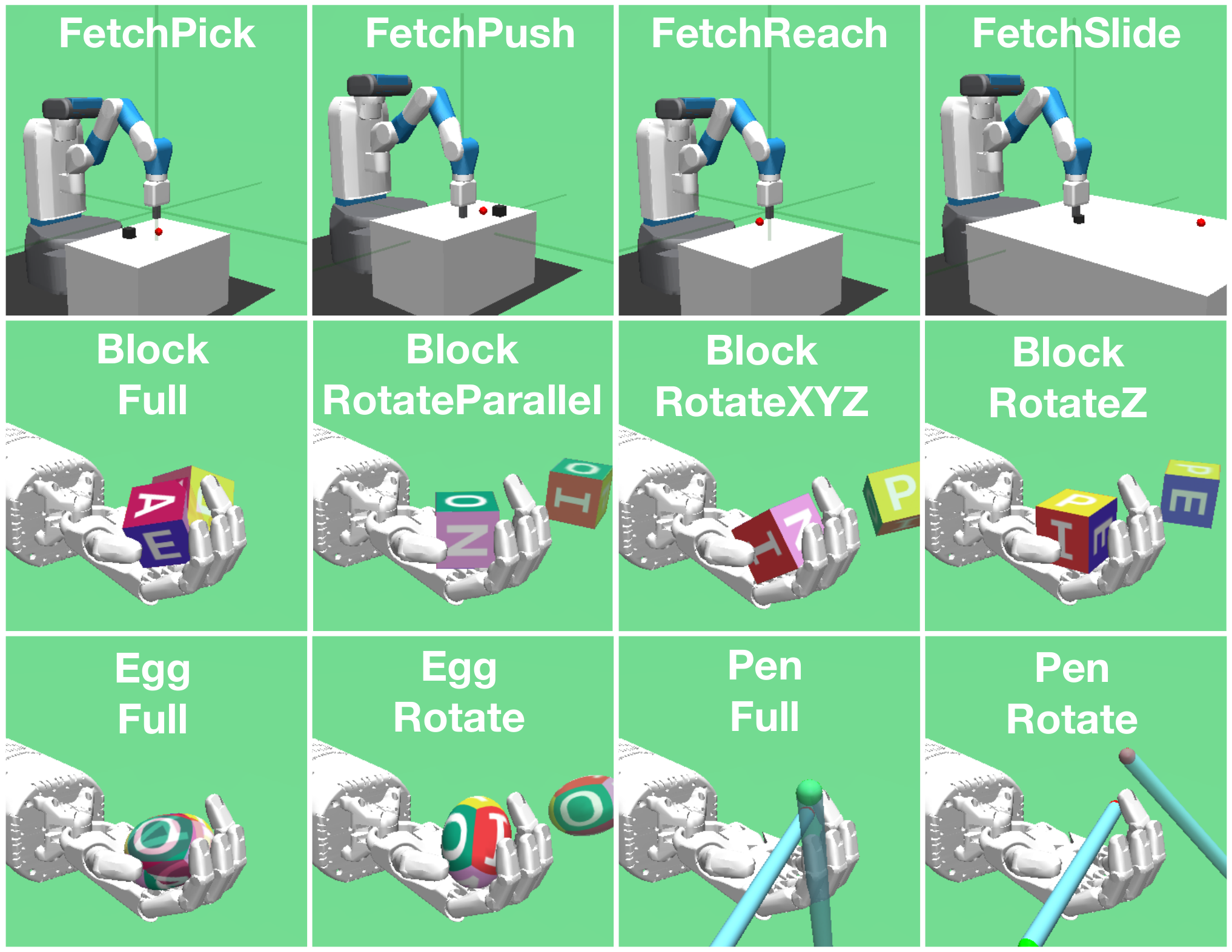
We use the standard GCRL benchmarks (Plappert et al. 2018) including all manipulation tasks on the Fetch robot and Shadow-hand (See Fig. 5).
Baselines
We compare MRN with a comprehensive list of existing UVFA architectures as illustrated in Fig. 1:
- •
Monolithic: is an unconstrained neural network that directly maps to the value.
- •
Bilinear Value Network (BVN) (Hong, Yang, and Agrawal 2022): .
- •
Deep/Wide Norms (DN/WN) (Pitis et al. 2020). DN/WN are networks that represent norm-induced metrics. The original DN/WN operates on the space where the metric is defined. To adapt them to the GCRL setting, we apply DN/WN to and with the same encoders as MRN.
- •
Poisson Quasi-metric Embedding (PQE) (Wang and Isola 2022). PQE represents quasi-metrics from a distribution perspective.
Algorithm and architecture
We use deep deterministic policy gradient (DDPG) (Lillicrap et al. 2015) with hindsight experience replay (HER) (Andrychowicz et al. 2017) as the base GCRL algorithm, within which we test all different architectures. Specifically, we only change the critic architecture . We constrain different networks to have the same number of parameters to equalize learning capacity. The monolithic network is a three-hidden-layer multi-layer perception (MLP) with 256 neurons per layer with ReLU activation (e.g. [linear-relu] + linear). BVN has two separate networks and , each of which is a three-layer MLP with 176 neurons per layer. For all other networks, we first define two encoders and (e.g. [linear-relu]). DN, WN, and PQE have method-specific modules on top of the two encoders, which follow the corresponding published implementation. For MRN, both the metric part and the residual asymmetric part are a single hidden layer neural network with 176 neurons (e.g., linear-relu-linear). The actor network is the same as the monolithic critic network except that the output layer projects to the action space.
Unified implementation on GPU
To our knowledge, there has not been a consistent codebase that compares all existing neural architectures for the GCRL problem. Moreover, past implementations with HER (Andrychowicz et al. 2017) require heavy CPU computation (e.g., 19 threads per run per environment). To address both issues, we implement all existing implementations in a unified framework and train fully on GPUs, which greatly reduces the amount of training time when extensive CPU computation is not available. The implementation only requires 2000 mebibytes (MiB) per run per environment. Across all architectures, we use the same learning rate of and the Adam optimizer (Kingma and Ba 2014) for updating both the actor and the critic.
Evaluation
For each architecture and each environment, we evaluate with 5 independent seeds . The agent is trained on 1000 episodes of data each epoch. After each training epoch, we evaluate the agent by recording its average performance (success rate) over 100 independent rollouts with randomly sampled goals. We plot the average success rate over learning epochs, averaged over the 5 seeds, along with its standard deviation (shaded region).
5.1 MRN Achieves Better Sample Efficiency
The GCRL experiment results using different state-of-the-art neural architectures as the critic is presented in Fig. 6. Note that within BVN, DN, WN, and PQE, no single method performs uniformly better than all other methods across all environments. By contrast, MRN (cyan) performs comparably to or better than all baseline methods in all environments.
5.2 On Importance of Both and
To validate the necessity of decomposing MRN into and , we conduct an ablation study that experiments with each part alone. To match the learning capacity, we enlarge the -only and -only networks to have 300 neurons per layer. The results are depicted in Fig. 7. From the figure, we can see that the -only network converges faster than the -only network. However, neither alone achieves the best sample efficiency or final performance. This result further confirms the necessity of combining both parts. To exclude the case that MRN outperforms the ablated networks due to the learning rate, we double the learning rate for the ablated methods, and the result is in Appendix C.1. Recall from Sec. 3.2 (and as illustrated in Fig. 1), that whereas in theory, is a function of , in practice, we only provide as inputs for the sake of efficiency. To validate this design, we check what happens when but . The result is in Fig. 7 (w/ SAG for e2). We observe that feeding all as input to confuses the network and prevents it from distinguishing between the roles of and .
6 Conclusion
This paper introduces the metric residual network for GCRL problems that has clear theoretical motivations and is straightforward to implement in practice. Comprehensive studies on standard GCRL benchmarks demonstrate that MRN outperforms all existing designs of neural architectures in terms of sample efficiency. As large models pretrained on a large set of environments become increasingly popular, we expect that investigating useful inductive biases for saving computation will become increasingly interesting and important. An interesting future research direction is to explore effective architectures for more general RL problems where the reward function can take an arbitrary form.
7 Acknowledgement
The research was conducted in both the statistical learning and AI group (SLAI) led by Qiang Liu and the Learning Agents Research Group (LARG) led by Peter Stone in computer science at UT Austin. SLAI research is supported in part by CAREER-1846421, SenSE-2037267, EAGER-2041327, and Office of Navy Research, and NSF AI Institute for Foundations of Machine Learning (IFML). LARG research is supported in part by NSF (CPS-1739964, IIS-1724157, FAIN-2019844), ONR (N00014-18-2243), ARO (W911NF-19-2-0333), DARPA, GM, Bosch, and UT Austin’s Good Systems grand challenge. Peter Stone serves as the Executive Director of Sony AI America and receives financial compensation for this work. The terms of this arrangement have been reviewed and approved by the University of Texas at Austin in accordance with its policy on objectivity in research. Special thanks to Xuchen Ma for the valuable discussion on goal-conditioned reinforcement learning.
References
- Andrychowicz et al. (2017) Andrychowicz, M.; Wolski, F.; Ray, A.; Schneider, J.; Fong, R.; Welinder, P.; McGrew, B.; Tobin, J.; Pieter Abbeel, O.; and Zaremba, W. 2017. Hindsight experience replay. Advances in neural information processing systems, 30.
- Borsa et al. (2018) Borsa, D.; Barreto, A.; Quan, J.; Mankowitz, D.; Munos, R.; Van Hasselt, H.; Silver, D.; and Schaul, T. 2018. Universal successor features approximators. arXiv preprint arXiv:1812.07626.
- Dayan (1993) Dayan, P. 1993. Improving generalization for temporal difference learning: The successor representation. Neural computation, 5(4): 613–624.
- Fujimoto, Hoof, and Meger (2018) Fujimoto, S.; Hoof, H.; and Meger, D. 2018. Addressing function approximation error in actor-critic methods. In International conference on machine learning, 1587–1596. PMLR.
- Haarnoja et al. (2018) Haarnoja, T.; Zhou, A.; Hartikainen, K.; Tucker, G.; Ha, S.; Tan, J.; Kumar, V.; Zhu, H.; Gupta, A.; Abbeel, P.; et al. 2018. Soft actor-critic algorithms and applications. arXiv preprint arXiv:1812.05905.
- Hong, Yang, and Agrawal (2022) Hong, Z.-W.; Yang, G.; and Agrawal, P. 2022. Bilinear value networks. arXiv preprint arXiv:2204.13695.
- Kingma and Ba (2014) Kingma, D. P.; and Ba, J. 2014. Adam: A method for stochastic optimization. arXiv preprint arXiv:1412.6980.
- Kulkarni et al. (2016) Kulkarni, T. D.; Saeedi, A.; Gautam, S.; and Gershman, S. J. 2016. Deep successor reinforcement learning. arXiv preprint arXiv:1606.02396.
- Lillicrap et al. (2015) Lillicrap, T. P.; Hunt, J. J.; Pritzel, A.; Heess, N.; Erez, T.; Tassa, Y.; Silver, D.; and Wierstra, D. 2015. Continuous control with deep reinforcement learning. arXiv preprint arXiv:1509.02971.
- Littman and Sutton (2001) Littman, M.; and Sutton, R. S. 2001. Predictive representations of state. Advances in neural information processing systems, 14.
- Mahadevan and Maggioni (2005) Mahadevan, S.; and Maggioni, M. 2005. Value function approximation with diffusion wavelets and laplacian eigenfunctions. Advances in neural information processing systems, 18.
- Pitis et al. (2020) Pitis, S.; Chan, H.; Jamali, K.; and Ba, J. 2020. An inductive bias for distances: Neural nets that respect the triangle inequality. arXiv preprint arXiv:2002.05825.
- Plappert et al. (2018) Plappert, M.; Andrychowicz, M.; Ray, A.; McGrew, B.; Baker, B.; Powell, G.; Schneider, J.; Tobin, J.; Chociej, M.; Welinder, P.; et al. 2018. Multi-goal reinforcement learning: Challenging robotics environments and request for research. arXiv preprint arXiv:1802.09464.
- Schaul et al. (2015) Schaul, T.; Horgan, D.; Gregor, K.; and Silver, D. 2015. Universal value function approximators. In International conference on machine learning, 1312–1320. PMLR.
- Singh et al. (2003) Singh, S. P.; Littman, M. L.; Jong, N. K.; Pardoe, D.; and Stone, P. 2003. Learning predictive state representations. In Proceedings of the 20th International Conference on Machine Learning (ICML-03), 712–719.
- Sutton and Barto (2018) Sutton, R. S.; and Barto, A. G. 2018. Reinforcement learning: An introduction. MIT press.
- Wang and Isola (2022) Wang, T.; and Isola, P. 2022. On the Learning and Learnablity of Quasimetrics. arXiv preprint arXiv:2206.15478.
Appendix A Theory
A.1 Proof of Thm. 2
Theorem 1.
Proof.
Assume the statement does not hold. As we fix the goals to be or , the GCRL problem is transformed into two standard MDPs with fixed goals. Therefore, there exists an optimal Markov policy for each problem. Specifically, denote optimal Markov policies corresponding to and as , and . Then consider the following policy for :
| (14) |
Here, denotes all past state and action pairs before time . Let be the random variable that indicates the first time reaches . Then we define
and
Then, clearly
| (15) |
The first equality follows the definition of . To see why the first inequality holds, note that
Similarly, we have
Combining above we can tell that the first inequality holds. The last inequality in Eq. (15) holds because of our assumption. Therefore, we have a policy (though possibly non-Markov) that achieves a higher expected discounted return with respect to reaching than , which contradicts the assumption that is optimal. ∎
A.2 Proof of Prop. 1
Proposition 1.
Assume , define
| (16) |
where is the Rectified Linear Unit (ReLU) function, and is a metric. Then ensures the three axioms of quasipseudometrics:
- •
Non-negativity:
- •
Identity:
- •
Triangle inequality:
Proof.
The non-negativity is obvious because is a metric and we use the ReLU function. The identity property can be easily checked. For the triangle inequality,
∎
A.3 Proof of in Eq. (11)
Assume the is attainable. Fixing a goal , the GCRL problem becomes the standard MDP and there exists a deterministic optimal policy for reaching from . Since we assume the dynamics is also deterministic, then it means the optimal trajectory to reach from is also deterministic. Denote this trajectory as where . Also denote
| (17) |
Then we argue that . Assume otherwise, then either or .
- •
:
this is impossible because otherwise we can replace with the policy corresponding to to reach a higher return, contradicting the definition of . - •
:
DenoteIn other words, is the first pair along that reaches the goal. Then there are two cases:
- –
After reaches , it will come back to again (hence repeatedly). In this case, clearly
contradicting our assumption that . The first inequality follows the definition of . The second inequality follows the definition of .
- –
After reaches , it will never come back to again. In this case, one can find the next . Then similarly there are two cases, if repeatedly visits , then we follow the argument in the above case. Otherwise we can recursively find the next , so on and so forth. Eventually, either we end up with the last state such that no satisfies , from which then we can see that
The last inequality follows that ever since we visit , all future rewards will be . Or the other case is that there exists an infinite length sequence of such . Then following this sequence, the original statement is still true though the is no longer attainable. But in this case, one can find a in the sequence such that is arbitrarily close to .
- –
A.4 Proof of Thm. 2
Theorem 1 (Universal approximation of ).
Given any continuous function , where is a quasipseudometric and is compact. Then , with a sufficiently large , there exists a quasipseudometric in the form of Eq. (12) such that
Proof.
First of all, from Prop. 1, any in the form of Eq. (12) is a quasipseudometric. Next we show that any quasipseudometric can be approximated by a in the form of Eq. (12). Since is a quasipseudometric, we have
| (18) |
As is continuous in both and , for a fixed pair of , define
| (19) |
Then is clearly continuous in (continuous functions are closed under subtraction and max operation). By definition of continuity,
| (20) |
where is a metric on . Since is compact, for a sufficient large , we can cover the domain with -radius balls centered at , i.e.
Now, consider the function , where for any ,
| (21) |
Denote , then we have ,
| (22) |
Clearly the defined above is in the form of Eq. (12) (we can set ). ∎
Appendix B Algorithm
The forward pass of MRN in PyTorch-like pseudocode is provided in Alg. 1. Here, , , and are standard multi-layer perceptrons (MLPs).
# The forward pass in PyTorch code
def forward(self, state, action, goal):
# state (batch, dim_state)
# action (batch, dim_action)
# goal (batch, dim_goal)
# 1. Projection
sa = torch.cat([state, action], -1)
sg = torch.cat([state, goal], -1)
x = self.e_1(sa)
y = self.e_2(sg)
# 2. Enforcing triangle inequality
d_sym = self.sym(x) - self.sym(y)
d_sym = d_sym.pow(2).mean(-1).sqrt()
d_asym = self.asym(x) - self.asym(y)
d_asym = F.relu(d_asym).max(-1)[0]
Q_sag = -(d_sym + d_asym).view(-1,1)
return Q_sag
Appendix C Experiment
C.1 Ablation study with doubled learning rate
We conduct the same ablation as in Sec. 5.1 except that we double the learning rate to . Results are shown in Fig. 8. From the figure, we can see that the claim in the main experiment section holds true.