A Sequence Tagging based Framework for Few-Shot Relation Extraction
Abstract
Relation Extraction (RE) refers to extracting the relation triples in the input text. Existing neural work based systems for RE rely heavily on manually labeled training data, but there are still a lot of domains where sufficient labeled data does not exist. Inspired by the distance-based few-shot named entity recognition methods, we put forward the definition of the few-shot RE task based on the sequence tagging joint extraction approaches, and propose a few-shot RE framework for the task. Besides, we apply two actual sequence tagging models to our framework (called Few-shot TPLinker and Few-shot BiTT), and achieves solid results on two few-shot RE tasks constructed from a public dataset.
1 Introduction
Relation Extraction (RE) is a fundamental task in natural language processing, aiming to extract the relation triples of the form in unstructured text. In a relation triple, and are the entities in the text, called the head entity and the tail entity respectively according to their positions. And describes the directed relationship from the head entity to the tail entity. Currently, the mainstream solutions follow the idea of joint extraction, which are mainly divided into the two methods: building up a label predicting system with a sequence tagging scheme (Zheng et al. 2017; Wei et al. 2020; Wang et al. 2020) and constructing a seq2seq system (Zeng et al. 2018; Nayak and Ng 2020; Zeng, Zhang, and Liu 2020). These systems have achieved solid results on the generic RE datasets with a sufficient amount of labeled instances.
However, one challenge remaining is that these RE systems based on the neural network require a lot of labeled training data, while the tagging effort is labor-intensive. The distant supervision method (Mintz et al. 2009) was proposed to obtain training data more cost-effectively. Based on existing knowledge graphs, the instances in the corresponding domain are automatically annotated. But a serious problem is that the samples labeled by the distant supervision method suffer from a large number of missed and incorrect tags. Thus the models must be reconstructed to accommodate these datasets with noise information. In addition, if there is no available knowledge graph for a particular domain, it is still impossible to complete the annotation for the training data.
As a result, researchers started to explore how to transfer knowledge from the resource-rich domains (such as the news domain) to the resource-poor domains (such as the medical domain). They worked to make the model achieve better results based on a small amount of labeled data in the target domain. Previously, they followed the simple pipeline idea and respectively assigned the knowledge transferred task to RE’s two sub-tasks, i.e. named entity recognition (NER) (Fritzler, Logacheva, and Kretov 2019; Hou et al. 2020; Yang and Katiyar 2020) and relation classification (RC) (Han et al. 2018; Gao et al. 2019; Baldini Soares et al. 2019). These works are all distance-based approaches, drawing on the classical few-shot approaches in the image field. However, the error propagation of pipeline is self-explanatory. Currently, the methods of few-shot NER and few-shot RC are not effective enough, let alone combining the two for RE.
Besides, the few-shot works in named entity recognition are essentially to find the closest label to a particular token of the input text. The idea is also applicable to the sequence label predicting systems in the joint extraction methods. Therefore, it is effective and feasible to apply the few-shot methods to joint extraction models.
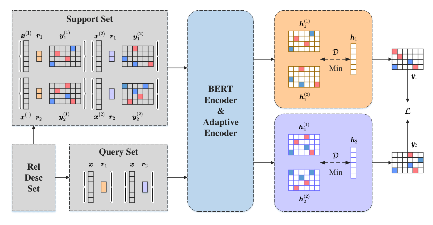
In this paper, we propose a method11 1 Available at https://anonymous/for/review. to combine a sequence tagging based model for joint extraction and the few-shot methods to improve the performance with limited target domain’s labeled data. In order to adopt the idea of distance-based few-shot sequence tagging to joint extraction methods, we begin with proposing a definition of the few-shot RE task through the sequence tagging based approaches. Second, we construct a sequence tagging based few-shot RE framework for the few-shot RE task. In our framework, the input instances are encoded by a BERT Encoder and an Adaptive Encoder, and then the distance between the hidden states of tokens and the labels are calculated, finally the predicted label sequence is outputted through distance comparison. Third, we apply two actual sequence tagging RE models (Wang et al. 2020; Luo et al. 2020) to the framework. These two models achieve solid results on two few-shot RE tasks constructed from a public dataset.
The key contributions are summarized as:
- •
The definition of the few-shot RE task based on the sequence tagging approaches is presented for the first time.
- •
A few-shot joint RE framework is developed for sequence tagging approaches, and two actual sequence tagging models is applied to the framework.
- •
An accelerated approximation scheme is proposed for calculating the distance matrices in the training phrase of Section 4.2.
2 Related Work
2.1 Relation Extraction
RE, as a sub-task of information extraction, is an important part of building knowledge graphs. Current research on supervised methods is becoming increasingly sophisticated.
Some supervised RE methods followed the pipeline ideas (Zeng et al. 2014; Xu et al. 2015; Vu et al. 2016; Zhong and Chen 2021), i.e., one model is used to recognize entities in a sentence, and then another model is used to identify the relations between each entity pair. The two models have different structures and parameters. Due to the error propagation problem of pipeline, other models turned to the joint method. They extracted entities and relations separately through two models that share parameters, or even simultaneously using a single model. For example, (Miwa and Bansal 2016; Katiyar and Cardie 2016) extended the relation classification module to share the encoder representation with the entity recognition module; (Zheng et al. 2017; Dai et al. 2019; Wei et al. 2020; Luo et al. 2020; Wang et al. 2020) took the extracting tasks as a sequence labeling problem, worked on proposing reliable tagging scheme that can reduce out relational triples; (Zeng et al. 2018; Nayak and Ng 2020; Zeng, Zhang, and Liu 2020) directly generated the triples by the seq2seq framework.
2.2 Few-shot Relation Extraction
The above supervised methods rely on a large amount of training data in the target domain. However, the labeling of relational triples in sentence is labor-intensive, resulting in frequent shortages of target domain’s training data. Thus, learning from limited new labeled samples, called few-shot relation extraction, is a non-trivial task. To simplify the task, previous researchers followed the pipeline idea, which is different from the few-shot joint RE work in our paper.
Few-shot NER
There are already a few approaches for Few-shot NER. An intuitive one is to extract cross-domain generic knowledge based on the source domain’s labeled data, and then utilize target domain’s limited data for knowledge migration. To carry on, Fritzler, Logacheva, and Kretov 2019 applied the prototypical network (Snell, Swersky, and Zemel 2017) for Few-shot NER, utilizing prototypes comparison to tag tokens. Hou et al. 2020 put forward the collapsed dependency transfer mechanism, adapting the traditional conditional random field (CRF) to the mutable entity label categories. Yang and Katiyar 2020 proposed the nearest neighbor comparison scheme and pre-trained the few-shot NER model by a standard supervised NER method. Tong et al. 2021 found and explored the rich semantics in class. And Ding et al. 2021 presented a practical and challenging dataset named Few-NERD for few-shot NER.
Few-shot RC
Given one entity pair that appear in a sentence, the RC task becomes a multi-classification problem. Han et al. 2018 were the first to formalize the definition of few-shot RC and proposed a new dataset called FewRel. They apply several few-shot learning methods to FewRel, e.g., prototypical network and meta network (Munkhdalai and Yu 2017). Gao et al. 2019 built up FewRel2.0 for few-shot RC with two real-world issues, i.e., few-shot domain adaptation and few-shot none-of-the-above detection. Baldini Soares et al. 2019 employed a simple prototype approach for a CNN-based system. What’s more, a more in-depth analysis (Brody, Wu, and Benton 2021) is performed on above works in a more realistic RE setting.
3 Problem Definition
In the sequence tagging based approaches of joint extraction, the label sequence can be obtained by a specific invertible tagging function , where is a sequence of tokens. indicates the set of relational triples in and is a specific relation category. Note that the numerical relationship between and is related to function from previous works, e.g., in (Zheng et al. 2017) and in (Dai et al. 2019).
Thus in few-shot RE, we intent to obtain a function . Here indicates a set of relation categories. And is called the support set, including relation categories (-way) and instances (-shot) for each category in the target domain. However, there may be multiple categories of triples in a single instance, making it difficult to sample from the source domain when training. To solve the problem, similar to (Ding et al. 2021), we introduce the -way -shot setting into few-shot RE task (Algorithm 1), i.e., a sampled contains instances for each relation category. Besides, is called the query set, which is the collection of the token sequences that need to be heuristically labeled according to . For simplicity, the number of instances in is assumed to be 1, i.e., . And is the prediction of the single instance in .
4 Methodology
In this section, we first present our sequence tagging based few-shot RE framework in general. Then we give two examples of how to apply the previous sequence tagging models for joint extraction to our framework, i.e., Few-shot TPLinker (Wang et al. 2020) and Few-shot BiTT (Luo et al. 2020).
4.1 Few-shot Relation Extraction Framework
As shown in Figure 1, our few-shot RE framework for sequence tagging approaches consists of the following 4 steps.
First, for each relation category, our framework needs to generate a label sequence by function for each instance in . For example, in Figure 1 is the label sequence derived from the instance in and the relation triple set in with relation category .
Second, each token sequence in and along with the description of a specific relation are input into a BERT Encoder (Devlin et al. 2019) to get the embedding of each token in , as follow.
| (1) |
Note that in Eq.(1) we utilize [SEP] as the concatenation token of and .
Third, for different sequence tagging models, our framework sets up an Adaptive Encoder, allowing models to obtain the hidden states for each position to be labeled that meet their own requirements.
| (2) |
Here the dimension of is , where is related to the tagging strategy and is the pre-defined hidden size. Note that the parameters of the Bert Encoder and the Adaptive Encoder can be pre-trained in advance with a traditional sequence tagging task in the source domain by appending a linear layer after and maximizing the probability of every correct label.
Finally, we compute the distance of the hidden state between each position of in and .
| (3) |
Here is the distance matrix, where means the instance number in . and are the hidden states of and respectively from Eq.(2). Besides, indicates the squared Euclidean distance function. Note that since is chunked in some specific tagging strategies, the distances between positions across chunks are not calculated to avoid the confusion of the labels in different chunks. For example, in TPLinker (Wang et al. 2020), there are three tagging matrices which contain different tags and represent different information. The labels sequence in a single matrix for all tokens is called a chunk and generated based on the TPLinker tagging strategy contains three chunks. For the inference stage, we utilize the label of the closest position in to a specific position in as ’s label, as follow.
| (4) | ||||
| (5) |
Here is the predicted label sequence of for the specific relation and indicates the mapping function from each position in to its label. And for the training stage, we assume that is divided into chunks of equal length. In a specific chunk with index , the distance between a position in and a label can be calculated by:
| (6) |
where indicates the set of all positions labeled with in the chunk of . Note that the chunk contains kinds of labels, i.e., . And we apply the cross entropy loss function for every chunk to minimize the distances between and the correct label, as follow.
| (7) | ||||
| (8) |
Here is the one-hot form of , which means the label index of the -th position in chunk of . The final loss is the average of .
4.2 Few-shot TPLinker

TPLinker (Wang et al. 2020) is an one-stage joint extraction model. It predicts three tagging matrices for the input instance, i.e., EH-to-ET, SH-to-OH and ST-to-OT. The elements in the matrices are selected in . Note that the label is proposed to reduce the matrix space by mapping the label in the lower triangular region to the upper triangular region. However, in the few-shot RE task, there may be no label in the tagging matrices of , making it hard to calculate the distance from the positions to be annotated to label . Therefore, we cancel this improvement when applying TPLinker to our framework. In this case, the length of the label sequence for a specific relation category is , and where . And the number of chunks in TPLinker is . The following describes the process for a single chunk of applying TPLinker to the sequence tagging based few-shot RE framework.
Adaptive Encoder
For the optimization of the next distance calculation step, we define the hidden state of (, ) as a concatenation of two parts, as follow.
| (9) |
Here and respectively denote the hidden states of the head token and the tail token . They are calculated by two linear layers:
| (10) | ||||
| (11) |

| Group | Categories | Instances Num | |||||
|---|---|---|---|---|---|---|---|
| A |
|
56,546 | |||||
| B |
|
14,942 | |||||
| C |
|
8,284 |
Distance Matrix
As shown in Figure 2, the distance between the token pairs (, ) in and (, ) in is divided into two part, as follow.
| (12) |
Here are distance matrices between the tokens in and . and are generated from and respectively by Eq.(3). Note that and belong to the same instance in . In Few-shot TPLinker, the distances from (, ) to label and label , called and , is required to be obtained respectively. If the solution is preformed by traversing all token pairs in , the overall time complexity for working out and can be . For example, as shown in the left part of Figure 2, all distances between (, ) and all token pairs in should be computed once, for a total of 16 times. Thus, we devise an accelerated approximation scheme in the training phrase. First, iterate over the positive samples set to fill as follow, since .
| (13) |
Second, assume that there is at least one negative sample among the top- tokens pairs with the shortest distance from (, ). These top- distances can be given by:
| (14) |
where , , and . and denote the distances respectively from ’s and ’s top- nearest tokens of the s-th instance in .
| (15) | ||||
| (16) |
Last, denote the set of values in except for as . can be roughly filled with the minimum (Eq.(17)) or average (Eq.(18)) value in . Thus the time complexity of our accelerated approximation scheme for and is .
| (17) | ||||
| (18) |
4.3 Few-shot BiTT
BiTT (Luo et al. 2020) is an end-to-end RE framework with the bidirectional tree tagging scheme. It predicts a label sequence containing the tree structures of the relational triples for an input sentence, and then reconstructs the relational graph to extract triples. In BiTT scheme, the chunk number is 8, and the length of is . The following introduces the procedure in a single chunk for adopting BiTT into our framework.
Adaptive Encoder
We define that the hidden state of is related to the embedding of by the following equation:
| (19) |
where is the weighted matrix and is the bias.
Distance Matrix
As shown in Figure 3, we calculate the distances from to the tokens in and work out the minimum distance for each label. Since there may not be any token with label , we calculate the distance between and a prototype inherited from previous training steps.
| (20) |
Here indicates the set of all tokens labeled with in the chunk of . Note that the update operation is executed only if .
5 Experiments
5.1 Dataset and Evaluation Tasks
Considering that different RE datasets are generated with different methods and relation category naming standards, it may face the issues of inconsistent relation descriptions and contradictory common knowledge when using multiple datasets for few-shot experiments. Moreover, it is practical to utilize a single dataset to perform different few-shot task scenarios, and then effectively validate the performance of our framework. Therefore, we evaluate Few-shot TPLinker and Few-shot BiTT on NYT (Zeng et al. 2014), an English RE dataset with 66,195 instances. NYT is labeled by the distant supervision method and a hierarchical naming standard. It pre-defines 24 fine-grained relation categories and 4 coarse-grained relation types.
Following the few-shot task setting of (Ding et al. 2021), we split the overall relation triple set into groups on consideration for the different granularity of category names. In this case, every group corresponds to a sub-dataset of instances containing the triples in the group. Besides, to avoid the observation of triples belonging to other groups, we need to mask out these triples first and then perform sequence tagging on the instances. Based on this setting, we develop two few-shot RE tasks adopting different splitting scheme and conduct 2-way 12-shot experiments on these tasks.
| Model | Group A | Group B | Group C | Average | ||||||||||||||||||||
|---|---|---|---|---|---|---|---|---|---|---|---|---|---|---|---|---|---|---|---|---|---|---|---|---|
| Prec | Rec | F1 | Prec | Rec | F1 | Prec | Rec | F1 | Prec | Rec | F1 | |||||||||||||
| No pretrain, no finetune | ||||||||||||||||||||||||
| Few-shot TPLinker (min) | 24.2 | 15.1 | 18.6 | 44.8 | 26.1 | 33 | 22.5 | 22.9 | 22.7 | 30.5 | 21.4 | 24.8 | ||||||||||||
| Few-shot TPLinker (avg) | 6.4 | 13.1 | 8.6 | 28.9 | 22.9 | 25.6 | 4 | 18 | 6.7 | 13.1 | 18 | 13.6 | ||||||||||||
| Few-shot BiTT | 47.7 | 12.9 | 20.4 | 51.6 | 14.4 | 22.5 | 23.6 | 8.3 | 12.3 | 41 | 11.9 | 18.4 | ||||||||||||
| Pretrain, no finetune | ||||||||||||||||||||||||
| Few-shot TPLinker (min) | 38.7 | 12.5 | 18.9 | 50 | 22.7 | 31.2 | 33.4 | 14.3 | 20 | 40.7 | 16.5 | 23.4 | ||||||||||||
| Few-shot TPLinker (avg) | 37.8 | 12.3 | 18.5 | 46.9 | 22.4 | 30.3 | 25.9 | 20 | 22.6 | 36.9 | 18.2 | 23.8 | ||||||||||||
| Few-shot BiTT | 63.9 | 10.5 | 18.1 | 64 | 22.8 | 33.6 | 53.4 | 6.4 | 11.5 | 60.4 | 13.2 | 21.1 | ||||||||||||
| Pretrain, finetune | ||||||||||||||||||||||||
| Few-shot TPLinker (min) | 21.3 | 18.7 | 19.9 | 50.1 | 33.6 | 40.2 | 37.3 | 24 | 29.2 | 36.2 | 25.4 | 29.8 | ||||||||||||
| Few-shot TPLinker (avg) | 43 | 17 | 24.3 | 48.5 | 31.5 | 38.2 | 25.9 | 20 | 22.6 | 39.1 | 22.8 | 28.4 | ||||||||||||
| Few-shot BiTT | 60.5 | 13.4 | 21.9 | 62.2 | 27.2 | 37.9 | 54.7 | 10.3 | 17.3 | 59.1 | 17 | 25.7 | ||||||||||||
Few-NYT (INTER)
In this task, we randomly and manually divide the 24 relation categories in NYT into group A, group B and group C. As shown in Table 1, every group is assigned 8 fine-grained relation categories, and the instances number of three sub-datasets are 56,546, 14,942 and 8,284 respectively. We do not consider the coarse-grained type to which each fine-grained relation category belongs. For example, /people/person/ethnicity, /people/person/place_lived and /people/person/children all belong to the coarse-grained type people, while they are separately partitioned into group A, group B and group C. In the experiments of this task, we take each group as the target domain for evaluating our models, and the remaining two groups as the source domain for training. In Few-NYT (INTER), our models may be more capable of mining the common knowledge between the source and target domains, since the three groups share some of the coarse information.
Few-NYT (INTRA)
In NYT, there are 4 predefined coarse-grained relation types, i.e., location, business, sports and people. When dividing these four relation types, we consider about the balance the amount of data in the training and validation sets, and also expect to mask out as few as possible relation triples. Thus, we simply adopt the instances set of location, business and sports as the training set, and the instances set of people as the validation set. The instances number of the training and validation sets are 51,559 and 16,711 respectively. In contrast to Few-NYT (INTER), the source and target domains of Few-NYT (INTRA) do not share coarse information as there is no intersection of coarse-grained relation types. Therefore, our models may be able to explore less inter-domain pervasive information, making this task more difficult.
5.2 Experimental Settings
Competitive Models
To the best of our knowledge, our Few-shot Relation Extraction Framework is the first few-shot system for joint extraction of entities and relations. Thus we do not choose other baselines, but construct three competitive models based on our framework for comparison experiments, as shown in Tabel 2 and Tabel 3.
- •
- •
- •
Few-shot BiTT: The Few-shot BiTT model mentioned in Section 4.3.
In addition, we design three training modes for these models to explore the effect of pre-training and fine-tuning on them. No pretrain, no finetune indicates that the models are trained directly from scratch based on the loss (Eq.(7)) of our few-shot RE framework. Pretrain, no finetune indicates that the models are only pre-trained in the traditional sequence tagging RE task, while not fine-tuned in the few-shot RE task. Pretrain, finetune indicates that the models are both pre-trained in the traditional sequence tagging RE task and fine-tuned in the few-shot RE task.
Parameter Tuning
In our framework, we adopt the default BERT-Based-Cased hyper-parameter values provided by Hugging Face22 2 https://huggingface.co/. Overall, in our experiments, the number of iterations for direct training and fine-tuning are 500,000 and 100,000 separately, and the number of epochs in pre-training is 20. In the process of direct training and fine-tuning, 5,000 iterations of validation are performed for every 10,000 iterations of training. In the pre-training process, we divide the data in the source domain into training set and validation set in the ratio of 4:1, and evaluate on the validation set after two training epochs. Then we save the pre-trained models with the best result. Besides, the batch size in pre-training process is set to 128, and the learning rate of Adam optimizer is 2e-5.
What’s more, there are a few hyper-parameters that need to be set artificially in the formulations elaborating our framework and models in Section 4. For our few-shot RE framework, in Eq.(1), the maximum length of the relation category description and the input tokens sequence are 10 (including [CLS] and [SEP]) and 50 (including [SEP]) respectively. And the relation category description is the word sequence obtained from the corresponding fine-grained relation category name by the tokenization based on the BERT-Based-Cased vocabulary. In Eq.(2), the hidden size of is . For few-shot TPLinker, in Eq.(10) and Eq.(11), the dimension of and is 76832. And is set to 3 in Eq.(14), Eq.(15) and Eq.(16). For few-shot BiTT, in Eq.(19), the dimension of is 76832. In Eq.(20), the hidden size is 32 and the weighted variable is set to 0.9.
Evaluation Metrics
The optimal models after training are evaluated on the target domain by 20,000 iterations of sampling. We report the standard evaluation metrics for RE: Precision (Prec), Recall (Rec) and F1 score (F1). We consider a predicted triple as a correct one only if , and are all correct.
5.3 Results
The experimental results on Few-NYT (INTER) and Few-NYT (INTRA) are shown in Table 2 and Table 3 respectively.
Models Comparison
As shown in Table 2, each of the three models based on our proposed Few-shot RE framework has its own benefits. First, Few-shot TPLinker (min) achieves the best average F1 (29.8%) and rec (25.4%) scores on Few-NYT (INTER), outperforms the second best model (Few-shot TPLinker (avg)) by 1.4% and 2.6% separately. This indicates that Few-shot TPLinker (min) works best overall and is able to recognize more valid relation triples in the target domain instances. Second, Few-shot TPLinker (avg) obtains the best F1 (24.3%) scores on Few-NYT (INTER) when we take group A as the target domain. It outperforms Few-shot TPLinker (min) by 4.4% and Few-shot BiTT by 2.4% in F1 respectively when the amount of instances (23,226) in the source domain is comparatively small. Third, Few-shot BiTT achieves the best average Prec (60.4%) score on Few-NYT (INTER), outperforms the second model (Few-shot TPLinker (min)) by 19.7%. This demonstrates that Few-shot BiTT tends to focus on the validity of its own predictions, rather than locating as many triples in the instance as possible. It is due to the fact that Few-shot BiTT only outputs a predicted triple when all tokens of both head entity and tail entity are consistently labeled.
| Model | Prec | Rec | F1 | |||
|---|---|---|---|---|---|---|
| No pretrain, no finetune | ||||||
| Few-shot TPLinker (min) | 2.2 | 3.3 | 2.6 | |||
| Few-shot TPLinker (avg) | 4.5 | 2.9 | 3.5 | |||
| Few-shot BiTT | 7.7 | 1 | 1.7 | |||
| Pretrain, no finetune | ||||||
| Few-shot TPLinker (min) | 22.8 | 3.2 | 5.6 | |||
| Few-shot TPLinker (avg) | 21.9 | 3.3 | 5.7 | |||
| Few-shot BiTT | 31.9 | 2.0 | 3.8 | |||
| Pretrain, finetune | ||||||
| Few-shot TPLinker (min) | 18 | 6.2 | 9.2 | |||
| Few-shot TPLinker (avg) | 39.8 | 5.1 | 9.1 | |||
| Few-shot BiTT | 20.2 | 1.9 | 3.5 |
The results in Table 3 also support the above conclusion on Few-shot TPLinker (min). Few-shot TPLinker(min) achieves the best F1 (9.2%) and rec (6.2%) scores on Few-NYT (INTRA), outperforms the second model (Few-shot TPLinker (avg)) by 0.1% and 1.1%. Few-shot TPLinker(avg) obtains the best Prec (39.8%) score, outperforms the second model (Few-shot BiTT) by 19.6%.
Effect of Pre-training
In our paper, we pretrain our encoders by appending a linear layer, and then perform softmax to achieve classification for each token. This operation can restrict the hidden state of tokens in the same class to a cluster, making the distance between these tokens small.
As demonstrated by comparing the results of part No pretrain, no finetune and part Pretrain, finetune in Table 2 and Table 3, pre-training enables the models to learn more knowledge related to RE, which greatly boosts the performance of our models. And the improvement is reliable in different few-shot task scenarios. On Few-NYT (INTER), Few-shot TPLinker(min), Few-shot TPLinker(avg) and Few-shot BiTT boost their average F1 score respectively by 5.0%, 14.8% and 2.7% after pre-training. On Few-NYT (INTRA), the three models boost their F1 separately by 6.6%, 5.6% and 1.8% after pre-training. In particular, on Few-NYT (INTER), the performance boost of Few-shot TPLinker(avg) is obvious. It indicates that the few-shot training of Few-shot TPLinker(avg) has a strict requirement on the parameters initialization, while pre-training optimizes the parameters by utilizing the knowledge of the sequence tagging RE task.
Effect of Fine-tuning
In our framework, the role of the loss in fine-tuneing stage is to further reduce the distance of intra-cluster tokens and increase the inter-cluster distance, thus increasing the probability of correctly classifying tokens on cluster boundaries.
Fine-tuning on the few-shot task based on pre-training has been proved to be a appropriate method to improve the generalization of our models. Comparing the results of part Pretrain, no finetune and part Pretrain, finetune in Table 2, Few-shot TPLinker(min), Few-shot TPLinker(avg) and Few-shot BiTT boost their average F1 score respectively by 6.4%, 4.6% and 4.6% after fine-tuning. However, experiments show that fine-tuning on the few-shot RE task may lead to overfitting in the source domain when the common knowledge between source and target domains is insufficient. For example, as shown in Table 3, on the Few-NYT (INTRA) task, the Prec, Rec and F1 of Few-shot BiTT separately decrease by 11.7%, 0.1% and 0.3% after fine-tuning.
Few-NYT (INTER) vs. Few-NYT (INTRA)
Since there is no overlap of coarse-grained relation types between the source and target domains in the Few-NYT (INTRA) task, our models is able to obtain less common information between the two domains, making it more difficult to extract triples. From Table 2 and Table 3, all models show a substantial decrease in performance on the Few-NYT (INTRA) task. Among them, Few-BiTT decreases the most, as evidenced by a significant drop in Prec and a tiny Rec. From this situation, it can be seen that the Few-BiTT model mainly learns information from the overlap of coarse-grained relation types. We conjecture that it is due to the fact that Few-BiTT needs to extract the tree structure embedded in the instance. While instances belonging to different coarse-grained types do not have similar relationship structures for Few-BiTT to learn.
6 Conclusion
In this paper, we put forward the definition of the few-shot RE task based on the sequence tagging approaches, and propose a few-shot RE framework for the task. Based on the few-shot RE framework, we construct three models called Few-TPLinker(min), Few-TPLinker(min) and Few-BiTT, and achieve solid results on Few-NYT (INTER) and Few-NYT (INTRA) tasks. Our future work aims to improve our frameork in two aspects, i.e. combining more category description information and exploring other ways to model the cross-domain knowledge.
References
- Baldini Soares et al. (2019) Baldini Soares, L.; FitzGerald, N.; Ling, J.; and Kwiatkowski, T. 2019. Matching the Blanks: Distributional Similarity for Relation Learning. In Proceedings of the 57th Annual Meeting of the Association for Computational Linguistics, 2895–2905. Florence, Italy: Association for Computational Linguistics.
- Brody, Wu, and Benton (2021) Brody, S.; Wu, S.; and Benton, A. 2021. Towards Realistic Few-Shot Relation Extraction. In Proceedings of the 2021 Conference on Empirical Methods in Natural Language Processing, 5338–5345. Online and Punta Cana, Dominican Republic: Association for Computational Linguistics.
- Dai et al. (2019) Dai, D.; Xiao, X.; Lyu, Y.; Dou, S.; She, Q.; and Wang, H. 2019. Joint Extraction of Entities and Overlapping Relations Using Position-Attentive Sequence Labeling. In Proceedings of AAAI, 6300–6308.
- Devlin et al. (2019) Devlin, J.; Chang, M.-W.; Lee, K.; and Toutanova, K. 2019. BERT: Pre-training of Deep Bidirectional Transformers for Language Understanding. In Proceedings of the 2019 Conference of the North American Chapter of the Association for Computational Linguistics: Human Language Technologies, Volume 1 (Long and Short Papers), 4171–4186. Minneapolis, Minnesota: Association for Computational Linguistics.
- Ding et al. (2021) Ding, N.; Xu, G.; Chen, Y.; Wang, X.; Han, X.; Xie, P.; Zheng, H.; and Liu, Z. 2021. Few-NERD: A Few-shot Named Entity Recognition Dataset. In Proceedings of the 59th Annual Meeting of the Association for Computational Linguistics and the 11th International Joint Conference on Natural Language Processing (Volume 1: Long Papers), 3198–3213. Online: Association for Computational Linguistics.
- Fritzler, Logacheva, and Kretov (2019) Fritzler, A.; Logacheva, V.; and Kretov, M. 2019. Few-Shot Classification in Named Entity Recognition Task. In Proceedings of the 34th ACM/SIGAPP Symposium on Applied Computing, 993–1000.
- Gao et al. (2019) Gao, T.; Han, X.; Zhu, H.; Liu, Z.; Li, P.; Sun, M.; and Zhou, J. 2019. FewRel 2.0: Towards More Challenging Few-Shot Relation Classification. In Proceedings of the 2019 Conference on Empirical Methods in Natural Language Processing and the 9th International Joint Conference on Natural Language Processing (EMNLP-IJCNLP), 6250–6255. Hong Kong, China: Association for Computational Linguistics.
- Han et al. (2018) Han, X.; Zhu, H.; Yu, P.; Wang, Z.; Yao, Y.; Liu, Z.; and Sun, M. 2018. FewRel: A Large-Scale Supervised Few-Shot Relation Classification Dataset with State-of-the-Art Evaluation. In Proceedings of the 2018 Conference on Empirical Methods in Natural Language Processing, 4803–4809. Brussels, Belgium: Association for Computational Linguistics.
- Hou et al. (2020) Hou, Y.; Che, W.; Lai, Y.; Zhou, Z.; Liu, Y.; Liu, H.; and Liu, T. 2020. Few-shot Slot Tagging with Collapsed Dependency Transfer and Label-enhanced Task-adaptive Projection Network. In Proceedings of the 58th Annual Meeting of the Association for Computational Linguistics, 1381–1393. Online: Association for Computational Linguistics.
- Katiyar and Cardie (2016) Katiyar, A.; and Cardie, C. 2016. Investigating LSTMs for Joint Extraction of Opinion Entities and Relations. In Proceedings of the 54th Annual Meeting of the Association for Computational Linguistics (Volume 1: Long Papers), 919–929. Berlin, Germany: Association for Computational Linguistics.
- Luo et al. (2020) Luo, X.; Liu, W.; Ma, M.; and Wang, P. 2020. BiTT: Bidirectional Tree Tagging for Joint Extraction of Overlapping Entities and Relations. CoRR, abs/2008.13339.
- Mintz et al. (2009) Mintz, M.; Bills, S.; Snow, R.; and Jurafsky, D. 2009. Distant supervision for relation extraction without labeled data. In Proceedings of the Joint Conference of the 47th Annual Meeting of the ACL and the 4th International Joint Conference on Natural Language Processing of the AFNLP, 1003–1011. Suntec, Singapore: Association for Computational Linguistics.
- Miwa and Bansal (2016) Miwa, M.; and Bansal, M. 2016. End-to-End Relation Extraction using LSTMs on Sequences and Tree Structures. In Proceedings of the 54th Annual Meeting of the Association for Computational Linguistics (Volume 1: Long Papers), 1105–1116. Berlin, Germany: Association for Computational Linguistics.
- Munkhdalai and Yu (2017) Munkhdalai, T.; and Yu, H. 2017. Meta Networks. In Proceedings of ICML.
- Nayak and Ng (2020) Nayak, T.; and Ng, H. T. 2020. Effective Modeling of Encoder-Decoder Architecture for Joint Entity and Relation Extraction. In Proceedings of AAAI.
- Snell, Swersky, and Zemel (2017) Snell, J.; Swersky, K.; and Zemel, R. 2017. Prototypical Networks for Few-shot Learning. In Proceeding of NeurIPS.
- Tong et al. (2021) Tong, M.; Wang, S.; Xu, B.; Cao, Y.; Liu, M.; Hou, L.; and Li, J. 2021. Learning from Miscellaneous Other-Class Words for Few-shot Named Entity Recognition. In Proceedings of the 59th Annual Meeting of the Association for Computational Linguistics and the 11th International Joint Conference on Natural Language Processing (Volume 1: Long Papers), 6236–6247. Online: Association for Computational Linguistics.
- Vu et al. (2016) Vu, N. T.; Adel, H.; Gupta, P.; and Schütze, H. 2016. Combining Recurrent and Convolutional Neural Networks for Relation Classification. In Proceedings of the 2016 Conference of the North American Chapter of the Association for Computational Linguistics: Human Language Technologies, 534–539. San Diego, California: Association for Computational Linguistics.
- Wang et al. (2020) Wang, Y.; Yu, B.; Zhang, Y.; Liu, T.; Zhu, H.; and Sun, L. 2020. TPLinker: Single-stage Joint Extraction of Entities and Relations Through Token Pair Linking. In Proceedings of the 28th International Conference on Computational Linguistics, 1572–1582. Barcelona, Spain (Online): International Committee on Computational Linguistics.
- Wei et al. (2020) Wei, Z.; Su, J.; Wang, Y.; Tian, Y.; and Chang, Y. 2020. A Novel Cascade Binary Tagging Framework for Relational Triple Extraction. In Proceedings of the 58th Annual Meeting of the Association for Computational Linguistics, 1476–1488. Online: Association for Computational Linguistics.
- Xu et al. (2015) Xu, Y.; Mou, L.; Li, G.; Chen, Y.; Peng, H.; and Jin, Z. 2015. Classifying Relations via Long Short Term Memory Networks along Shortest Dependency Paths. In Proceedings of the 2015 Conference on Empirical Methods in Natural Language Processing, 1785–1794. Lisbon, Portugal: Association for Computational Linguistics.
- Yang and Katiyar (2020) Yang, Y.; and Katiyar, A. 2020. Simple and Effective Few-Shot Named Entity Recognition with Structured Nearest Neighbor Learning. In Proceedings of the 2020 Conference on Empirical Methods in Natural Language Processing (EMNLP), 6365–6375. Online: Association for Computational Linguistics.
- Zeng et al. (2014) Zeng, D.; Liu, K.; Lai, S.; Zhou, G.; and Zhao, J. 2014. Relation Classification via Convolutional Deep Neural Network. In Proceedings of COLING 2014, the 25th International Conference on Computational Linguistics: Technical Papers, 2335–2344. Dublin, Ireland: Dublin City University and Association for Computational Linguistics.
- Zeng, Zhang, and Liu (2020) Zeng, D.; Zhang, R. H.; and Liu, Q. 2020. CopyMTL: Copy Mechanism for Joint Extraction of Entities and Relations with Multi-Task Learning. In Proceedings of AAAI.
- Zeng et al. (2018) Zeng, X.; Zeng, D.; He, S.; Liu, K.; and Zhao, J. 2018. Extracting Relational Facts by an End-to-End Neural Model with Copy Mechanism. In Proceedings of the 56th Annual Meeting of the Association for Computational Linguistics (Volume 1: Long Papers), 506–514. Melbourne, Australia: Association for Computational Linguistics.
- Zheng et al. (2017) Zheng, S.; Wang, F.; Bao, H.; Hao, Y.; Zhou, P.; and Xu, B. 2017. Joint Extraction of Entities and Relations Based on a Novel Tagging Scheme. In Proceedings of the 55th Annual Meeting of the Association for Computational Linguistics (Volume 1: Long Papers), 1227–1236. Vancouver, Canada: Association for Computational Linguistics.
- Zhong and Chen (2021) Zhong, Z.; and Chen, D. 2021. A Frustratingly Easy Approach for Entity and Relation Extraction. In Proceedings of the 2021 Conference of the North American Chapter of the Association for Computational Linguistics: Human Language Technologies, 50–61. Online: Association for Computational Linguistics.