Higher-order accurate two-sample network inference and network hashing
Abstract
Two-sample hypothesis testing for network comparison presents many significant challenges, including: leveraging repeated network observations and known node registration, but without requiring them to operate; relaxing strong structural assumptions; achieving finite-sample higher-order accuracy; handling different network sizes and sparsity levels; fast computation and memory parsimony; controlling false discovery rate (FDR) in multiple testing; and theoretical understandings, particularly regarding finite-sample accuracy and minimax optimality. In this paper, we develop a comprehensive toolbox, featuring a novel main method and its variants, all accompanied by strong theoretical guarantees, to address these challenges. Our method outperforms existing tools in speed and accuracy, and it is proved power-optimal. Our algorithms are user-friendly and versatile in handling various data structures (single or repeated network observations; known or unknown node registration). We also develop an innovative framework for offline hashing and fast querying as a very useful tool for large network databases. We showcase the effectiveness of our method through comprehensive simulations and applications to two real-world datasets, which revealed intriguing new structures.
Keywords: Network analysis, higher-order accuracy, nonparametric statistics, degeneracy, false-discovery rate
1 Introduction
The relational nature of network data presents unique challenges to data analysts. It is therefore very intriguing to ask how to extend statistical concepts, tools and theory in the classical i.i.d. setting to network settings. Levin and Levina 2019 said well: “A core problem in statistical network analysis is to develop network analogues of classical techniques.” Indeed, recent years have witnessed significant developments of network analysis toolbox for both point estimation (Abbe 2017) and one-sample inference (Gao and Lafferty 2017a; Banerjee and Ma 2017; Green and Shalizi 2022; Jin et al. 2018; Levin and Levina 2019; Zhang and Xia 2022). Comprehensive theoretical analysis of these tools has deepened our understanding of their statistical behaviors and performances. This paper studies a challenging and under-explored topic: two-sample network comparison. Spoken in plain language, the scientific question is how to compare two network models and based on their respective observations and . Though being challenging in general, this problem can be made easier by imposing two popular assumptions. The first popular assumption is repeated network observations, that is, and possibly even diverge, such as Ginestet et al. 2017; Ghoshdastidar and Von Luxburg 2018; Kolaczyk et al. 2020; Ghoshdastidar et al. 2020; Chen et al. 2022+; Maugis et al. 2020; Bravo-Hermsdorff et al. 2021; Yuan and Wen 2021. This assumption is particularly strong in that it implicitly assumes repeated network observations within each group are identically distributed. However, many real-world data sets clearly exhibit within-group heterogeneity. Consider the schizophrenia data in Section 9.2. Our analysis discovers subgroups within the patient and healthy people groups as shown in Figure 8. This is a clear evidence against the i.i.d. assumption on all patients’ brain networks. The second popular assumption states that all networks share a common node set, with known node correspondence, including Ghoshdastidar and Von Luxburg 2018; Li and Li 2018; Ghoshdastidar et al. 2020; Chen et al. 2022+. This assumption is sensible in some applications such as networks between the same set of participants, but it is restrictive in general. For instance, this assumption is true for the brain image data we shall analyze in Section 9.2, but not for the Google+ data in Section 9.1, where we compare ego-networks of different individuals, which, not only have no node correspondence, but also may vary greatly in network sizes. Two-sample network comparison becomes most challenging in the absence of the aforementioned two assumptions, namely, and there is no available node correspondence. Prior works typically require additional strong structural assumptions such as low-rankness or strict degree monotonicity (Tang et al. 2017; Agterberg et al. 2020; Yang et al. 2014; Sabanayagam et al. 2021). Moreover, most of these methods depend on strong modeling assumptions such as low-rankness with a known rank and equal network sizes with a known registration between the node sets of any two networks.
In this work, we propose a novel framework based on the network method-of-moments which can effectively tackle various challenges for network two-sample test. The highlights of our contributions are as follows. First, we present the first two-sample test procedure with higher-order accurate control of type-I error under the non-degeneracy assumption, a frequently met condition in many network data sets. Our method requires far less restrictive structural assumptions and can handle a much wider range of different sizes and sparsity levels than SVD-based methods; and outperforms other network-moment-based methods, such as network bootstraps, in finite-sample risk control accuracy.
Second, our method does not require repeated network observations or known node registration. However, the pooled version of our method can effectively leverage such available information to improve statistical efficiency. Its high versatility in handling various data types, combined with the higher-order accuracy of our inference formula, set our method apart from existing techniques. Moreover, our one-on-one comparison procedure remains a vital tool for detecting in-group heterogeneity, even with multiple observed networks in each group. It plays a crucial role in assessing the validity of pooling networks, addressing a key concern often overlooked in prior studies on comparing groups of networks.
Third, our method enjoys considerable speed advantages in one-on-one test over most existing methods, except for the normal approximation that we also studied in this paper. For multiple comparisons, we propose an innovative “network hashing + fast query” procedure. In the first stage, each network is precomputed into a concise vector of summary statistics; then in the second stage, we run our test using only these statistics. Our novel framework is particularly beneficial for large network databases, as it streamlines maintenance, boosts query speeds, and improves data privacy protection. While this framework can also enhance several existing methods, its combination with the test we propose in this paper achieves unrivaled memory efficiency after stage 1 and computational speed in stage 2 when facing a large number of queries.
Fourth, our paper also addresses several key issues that previous works have largely overlooked. The first challenge is computation, which becomes increasingly expensive as motif size grows. Another critical problem in practice is handling degeneracy, which remains blank in existing literature on network two-sample test. We propose a pioneering method in Section 6.2, leveraging recent advances in reduced U-statistics (Shao et al. 2023), to both speed up computation and adapt automatically to indeterminate degeneracy. Additionally, we address the unexplored problem of false discovery rate (FDR) control in multiple network comparison tests. We develop the first provably valid FDR control procedure for the network database query problem, filling a significant gap in the field.
Fifth, our theoretical studies provide rigorous guarantees of all the aforementioned methodological developments in this paper. Our results are much sharper than counterparts in existing literature. Furthermore, we present the first lower-bound result (Theorem 3) that delineates the finite-sample fundamental limit in test power and show that our method achieves power-optimality.
In summary, this paper substantially enhances and enriches the existing methodology toolbox and deepens the theoretical understanding of the performance and fundamental limits of network method-of-moments.
2 Graphon model and network moments
2.1 Two-sample graphon model
For narrative simplicity, we state our method and theory for unweighted, undirected networks with no self-loop, but these specifications are not essential. We observe two independent networks with and nodes, respectively, represented by their adjacency matrices and , where and . Throughout this paper, we choose graphon model as our base model. Graphon is a very general wrapper around many famous and widely-used network models (Gao et al. 2018; Young and Scheinerman 2007; Hunter et al. 2008; Bickel and Chen 2009; Olhede and Wolfe 2014). Our method, though designed to work for graphons, also works for these models as special cases. The data generation mechanism is as follows. First, assign a latent position to each node: Uniform. Second, there exists a latent, symmetric graphon function encoding all network structures, and a sparsity parameter , such that the edge probability between is . We inherit the regularity condition for model identifiability from Olhede and Wolfe 2014. Similarly define and . Finally, our observation is generated according to for all . Similarly define , , and generate . General audience may wonder if one can estimate , ’es and ’s and use them to compare network structures. Unfortunately, are only identifiable up to equivalent classes (Olhede and Wolfe 2014; Gao et al. 2015; Zhang et al. 2017). The edge probability matrices are fully identifiable, so one naturally considers a graph-matching-based network comparison. However, graph matching is a difficult problem even with structural assumptions (Lyzinski et al. 2015; Arroyo et al. 2021), and it typically requires rather costly computation.
2.2 Network method of moments
Our approach is to compare network moments, namely, the frequencies of patterned motifs, e.g. edges, triangles, star-shapes and circles (Bickel et al. 2011; Jin et al. 2018; Levin and Levina 2019). The idea is naturally inspired by its counterpart in classical statistics, where we compare the means, variances and other numerical features of two populations. Network method of moments enjoys high computational speed and memory efficiency (Zhang and Xia 2022). Particularly conveniently, they are invariant under node permutations, which exempts our approach from a slow and difficult graph matching step and easily enables it to handle different network sizes. Interestingly, two potentially very different network models may still share some common numerical features of scientific importance and interest. This is exactly analogous to the understanding in the classical two-sample test. Moreover, by (Zhao 2023, Corollary 5.49), the edit distance between two graphon models can be controlled by finite many moment distances. Therefore, our devised toolbox provides more flexibility than existing tools that test the exactly equality of two network models under restrictive structural assumptions.
Now we formally define network moments. Let denote a given motif of nodes and edges. Throughout this paper, we always assume the motif is connected. Following the tradition of Bickel et al. 2011; Zhang and Xia 2022; Maugis et al. 2020, for any -node graph , define if there exists bijection ; otherwise . The empirical network moment indexed by for network is
where we omit the dependency of and on to simplify notation. Here denotes the sub-matrix with row and column indices from the set . Denote the corresponding population moment by , where the expectation is taken w.r.t. the randomness of both network edges and latent positions. Similarly define and for network .
Notice that, however, the moments , are impacted by network sparsity measures , , and , respectively. Here the empirical network sparsity is define by
and similarly. Networks may exhibit very different sparsity levels (Decelle et al. 2011). To rule out the nuisance of network sparsity, similar to Bickel et al. 2011; Bhattacharya et al. 2022, we consider the Horvitz–Thompson estimators when designing the population discrepancy measure, which is defined as
Our central goal is to perform inference on . For instance, means that the two networks are possibly generated from the same network model (except sparsity levels), which can be of great scientific values in practice. A natural point estimator of is the plug-in version defined by
| (1) |
The main task is then to characterize the distribution of , for which its variance estimate is necessary so that it can be studentized. In Zhang and Xia 2022, the one-sample counterpart of our inference method is simply based on the studentized version of empirical moment where the underlying latent network sparsity only plays a role in theoretical analysis but does not appear in the method formulation. In sharp contrast, the network sparsities are indispensable in our designed estimator (1). As a result, a higher-order accurate characterization of the distribution of must carefully handles the estimation error induced by and , which will also interact with the estimation error in and . Moreover, the networks can have drastically different sizes and sparsity levels. All of this should reflect in the Edgeworth expansions. thus the one-sample result in Zhang and Xia 2022 needs significantly nontrivial extensions to suit our purpose.
3 Higher-order accurate method by Edgeworth expansion
3.1 Variance estimation and studentization
We quickly outline this section’s contents. We first estimate and use it to studentize ; this is nontrivial as variance estimators that require repeated network observations such as Maugis et al. 2020; Bravo-Hermsdorff et al. 2021 cannot function here. Then we studentize and formulate a higher-order accurate distributional approximation. This formulation then leads to our novel network offline hashing and fast querying toolbox. We also formulate the Cornish-Fisher confidence interval by inverting the CDF approximation. We conclude this section with our theorems that establish finite-sample accuracy and minimax optimality.
We now brief the rationale in our designed estimator of . Readers not interested in technical details may skip to eq. (3). To estimate , we decompose the stochastic variation in as follows:
| (2) |
where we define and . Note that the random variables and are classical noiseless U-statistics of degrees 2 and , respectively. Their randomness is exclusively driven by the latent positions ; thus they admit Hoeffding’s decompositions (Hoeffding 1948):
respectively. Here we slightly abuse notation and write . The Hoeffding’s decomposition terms are defined by , . The notation adopted here is slightly different from the conventional in literature. Basically, we write if for some absolute constant .
From eq. (2), the variation in originates from that in , and . It turns out (by the proof of Theorem 1) that when , the variation contributed by and are dominated by that in and . In fact, terms and are both dominated by a weighted average of terms, which encodes the randomness of network edges. Note that contains a remainder term while does not. Putting these understandings together, we have
| (3) |
where . The -index counterparts and are defined in the same fashion so that the variance of can be decomposed accordingly. The variance decomposition (3) is the foundation for us to estimate the variance of . We set throughout this paper, which is a fairly mild condition of network sparsity. Then we write , where we design the empirical version of via
Here the empirical versions of and are defined as follows:
The -indexed counterparts and are defined similarly. We are now in position to estimate by
| (4) |
Finally, we studentize as follows
| (5) |
One can equivalently use jackknife (Maesono 1997) to design , but our design is more convenient for analysis and faster to compute; see Theorem 3.3 in Zhang and Xia 2022 and the paragraph beneath it.
3.2 Characterizing the distribution via Edgeworth expansion
In this section, we present Edgeworth expansions as a higher-order accurate means to approximate , i.e., the c.d.f. of . To start, we set up some auxiliary quantities as building bricks of the coefficients in our expansion formula. Define the second-order terms in Hoeffding decomposition
and similarly define . Moreover, we set their variances and covariance by
Recall we defined in Section 3.1. The higher-order accurate characterization of requires auxiliary quantities , , , and , . Due to page limit, we sink their formal definitions to Section 11 in Supplementary Material. Define , , , , through similarly for graphon . The formal definitions of to and to are involved, but they are all and can be fast calculated empirically. Similarly, the quantities and are all . Note that we focus on the non-degenerate case where . We address degeneracy in Section 6.2.
Denote and the density and distribution function of a standard normal random variable. The higher-order accurate characterization of is decided by the following Edgeworth expansion (population version)
| (6) |
where the expansion terms are defined by
Here we write and , both of which are . Therefore, , and all of , and are . They characterize the first order terms in Edgeworth expansion. Basically, the goal is to show that approximates the distribution of (up to certain continuity correction to be clarified soon) with an accuracy sharper than , i.e., more precise than a Berry-Esseen bound. The following Theorem 1 confirms that such a higher-order accuracy can be achieved by under mild conditions.
The population version is not immediately applicable since it involves unknown quantities like , and so on. Fortunately, all these quantities can be accurately estimated and fast computed. Due to space limit, the definitions of corresponding estimators are relegated to Section 11 in the Supplementary Material. These estimators lead to empirical Edgeworth expansion terms , and . The empirical Edgeworth expansion (EEE) is defined by replacing , and by their estimators in . It is worth noting that all the involved quantities are computed separately for network or network , respectively, and no cross-network quantity is needed.
There are cases in which and admit discrete-type distributions (see (Zhang and Xia 2022) fore more discussions). If that happens, the dominating terms in such as are discrete-type random variables, and it becomes generally impossible to achieve the higher-order approximation to a discrete-type distribution by a continuous function like . A common assumption in the analysis of Edgeworth expansion of noiseless and noisy U-statistics is the Cramér’s condition. Zhang and Xia 2022 discovered that the observational errors in networks can contribute a surprising self-smoothing effect that waives the Cramér’s condition in most cases, but it does not cover very dense networks. In the context of this paper, this corresponds to assuming that either or for network ; and a similar assumption for network . Here, we propose a simple remedy that completely waives Cramér’s condition. Let be an artificial Gaussian noise term independent of the observed data with a sufficiently large constant . Simply put, the artificial Gaussian noise is strong enough to smooth the potentially discrete distribution of the dominating terms in . We shall use instead of for statistical inference.
We call acyclic if it is a tree; otherwise call it cyclic. The approximation accuracy of Edgeworth expansion depends on both the network size and sparsity level. More precisely, it is characterized by
| (7) |
We can define similarly for network B. We now present our main theorem. Note that the Kolmogorov distance is defined by .
Theorem 1 (Population and empirical Edgeworth expansions).
Assume:
- 1.
Network sizes satisfy: ;
- 2.
Network sparsities satisfy: and if is acyclic; and and if is cyclic.
- 3.
Non-degeneracy: .
Define the population Edgeworth expansion for as in (6). Let be its empirical version defined above. Then we have
| (8) | ||||
| (9) |
Theorem 1 addresses a much wider range of than all existing similar works. For example, Ghoshdastidar et al. 2017 assumes ; and Agterberg et al. 2020 makes the restrictive assumption that constant for dense networks or constant for sparse networks. Moreover, under the same parameter configuration assumptions, our method achieves much stronger results. For instance, under the settings of Ghoshdastidar et al. 2017, our eq. (9) gives a higher-order accurate distribution approximation error bound; to our best knowledge, this is the first result of its kind. Note that eq. (8) also implies the canonical Berry-Essen bound under appropriate network sparsity conditions. The network sparsity requirement in Theorem 1 matches those in the classical literature on network method-of-moments (Bickel et al. 2011; Bhattacharyya and Bickel 2015). Also, compared to other approaches to improve risk control accuracy such as iterative bootstrap (Hall and Martin 1988; Beran 1987; Beran 1988), which though has not yet been formulated for the network setting, our empirical Edgeworth expansion method computes much faster and has a much better provable error bound.
3.3 Two-sample test and Cornish-Fisher confidence interval
We now present our approach to two-sided test. Parallel results for one-sided alternatives can be easily derived. Our goal is to test
| (10) |
The empirical p-value produced by our method is
where we define the observed statistic by . Given a significance level , we reject the null hypothesis if and do not reject otherwise.
We also formulate the Cornish-Fisher confidence interval by inverting the Edgeworth expansion. Define to be the true lower- quantile of the distribution of . We can approximate by where . The two-sided Cornish-Fisher CI for estimating is
| (11) |
The higher-order accuracy of our distribution approximation leads to accurate controls of type-I error in the hypothesis test and the confidence level associated with the confidence interval.
Theorem 2.
The next theorem shows that our method, while enjoying higher-order accurate risk controls, simultaneously achieves minimax optimality.
Theorem 3.
- 1.
(Rate-optimality of the separation condition of our test) For any fixed , there exists population models:
- *
Under network 1 , network 2 ;
- *
Under network 1 , network 2
for some , , , , , such that under , while any procedure for the hypothesis test (10) suffers
(12) for some constant as .
- *
- 2.
(Rate-optimality of the expected length of our confidence interval) For any fixed ,
(13) for some constant .
Remark 1.
By Theorem 2 and Theorem 3, respectively, our method enjoys both higher-order accurate risk control and power-optimality. Importantly, we emphasize that achieving either of these two desirable properties is not difficult. For instance, a simple normal approximation also enjoys the optimality properties in Theorem 3, but not that in Theorem 2. However, achieving both higher-order accurate risk control and power-optimality, is challenging. To our best knowledge, our method is the first to provably achieve both.
4 Network hashing and fast querying
Suppose we query 11 1 The goal is to search for a network in a large database of networks that, potentially, is generated similarly as ignoring the possibly different sparsity levels and network sizes. a graph in a graph database that contains network entries of sizes and sparsity parameters , respectively. Here any or all of could potentially be very large. Our method effectively addresses this challenge by hashing database entries (each entry corresponds to a network) with offline computation into just a few summary statistics. When querying a keyword (network) , we only need to compare the hash of to entries’ hashes. This provides a very fast screening algorithm to quickly narrow down the search range. Our hashing-query procedure also protects data privacy, since all parties only need to disclose network summary statistics, not the entire networks. The fast speed and enhanced privacy may cater to the urgent needs of multi-institutional clinical research collaboration on Alzheimer (Chen et al. 2022) and other diseases, where privacy protection and high communication cost are two paramount concerns when sharing sensitive patient-level data (Chen et al. 2022). Using our method, researchers can conveniently build, maintain and query a large similarity graph between patient brain images across multiple hospitals for disease subtyping with improved privacy protection and high communication efficiency. We do clarify that mathematical quantification of privacy protection would be an interesting future work but not the purpose of this paper.
Input: Network database:
Output: Each hashes into a short vector of its own summary statistics
Steps:
For and for each motif, compute and output
and defined earlier; and
,
,
,
,
,
using
Section 11 of Supplementary Material.
Also output the motif name and .
Input: Queried “keyword” network ; Hashed database (output of Algorithm 1); level
Output: A list of ’s with similar network moments to ; or “not found” (empty query result)
Steps:
- 1.
Compute and defined earlier; and , , , , , using Section 11 of Supplementary Material using .
- 2.
- 3.
Extract entries satisfying as candidates passing our screening algorithm, whose match with the queried entry is to be further inspected.
Algorithms 1 and 2 show the offline nature of our hashing procedure, which can prepare database entries for fast query without knowing the queried keyword. This is very different from most existing methods such as Ghoshdastidar et al. 2017; Tang et al. 2017; Agterberg et al. 2020, which do not have a hashing stage and their query methods unavoidably require at least cross-computation, where is the size of the queried keyword network. The hashing cost on each individual entry is , see Section III.A of Ahmed et al. 2015. To see the distinction in computational cost, suppose all entries have same sizes and density levels and there are incoming queries. Then our method costs . In sharp constrast, existing methods that requires cross-computation cost , which will soon burn out the query system as becomes very large.
Next, we give a finite-sample error bound for type I and type II query errors.
Theorem 4.
Our proposed network hashing framework can also benefit several existing methods. However, these methods cannot match our approach in terms of memory efficiency and query speed22 2 In this scenario, hashing is computed only once, while the speed of handling continually incoming queries is the paramount concern. For the computation cost in the hashing stage: SVD methods require ; our method costs (full computation) or (reduced computation, see Section 6.1) for each motif; bootstraps need at least times the total cost of our method.. Let us first consider memory cost. For each network, after stage 1, SVD-based methods such as Agterberg et al. 2020 require memory, where is the network model’s known rank; bootstrap methods need memory, with being the number of bootstrap iterations; the cost is shared by ad-hoc inference procedures for other benchmarks (Wills and Meyer 2020; Tsitsulin et al. 2018), as they also utilize bootstrap. As Zhang and Xia 2022 highlights, to maintain accurate inference, bootstrap methods must increase at least as fast as increases. In stark contrast, our method requires only memory, where is the number of motifs considered, which can either stay fixed or grow rather slowly. Then we compare their query speeds. SVD-based methods are very slow due to their required cross-term computations – they cost ; bootstraps cost ; whereas our method only costs . This shows our method’s clear superiority in both memory and computational costs.
5 Pooling over multiple networks in the same group
As introduced in Section 3, our study initially focuses on the challenging scenario of , where each group has only one observed network. This prompts the question: can our method be adapted for less challenging scenarios where and/or exceed 1? Although our method can be applied in a one-on-one manner across tests, an extension that allows group-wise pooling would more effectively exploit available information in practice, when networks within a group are known to originate from the same model. To simplify presentation, we assume that all networks in group not only share the same graphon function but also have identical density adjustments and network sizes ; the same goes for group . While relaxing this simplifying assumption is not difficult, it would significantly complicate the formulas. We differentiate between two sub-cases: (i) networks in the same group sharing a common node set, and (ii) networks in each group independently generating their own node set.
5.1 Common node set
When networks share a common set of nodes, it is natural to assume that these nodes have identical latent positions across all networks. This implies a shared common probability matrix for all adjacency matrices. A natural treatment is to average the adjacency matrix as follows:
| (15) |
and use to estimate and . Denote the estimators as and , defined by:
| (16) |
In comparison to and from the case, following Zhang and Xia 2022 and this paper’s methodology, we decompose the variations in into two components: one due to randomness in and the other attributable to edge-wise observational errors. Remarkably, the formula of our method is calculated based on the first component, which remains unaffected by pooling. Therefore, no modifications to our algorithm are required, other than using as the input instead of in the case; the same applies to group . Theoretically, as anticipated, pooling modifies the error term.
Theorem 5.
With a fixed , the term in (17) does not vanish as , because it stems from the noiseless U-statistic part in the decomposition of the test statistic. This variation cannot be suppressed by repeated network observations, since these networks all share the same .
5.2 Independently selected node sets
6 Computation acceleration and adapting to degeneracy
6.1 Computation acceleration by U-statistic reduction
Computing a network moment for nodes and edges on a single network has a computational cost of . This is notably higher compared to low-rank decomposition methods, which cost with a known rank (Tang et al. 2017), particularly when and slowly diminishes. To speed-up our method, we use the U-statistic reduction technique (Chen and Kato 2019; Shao et al. 2023). For a tuning parameter , let be randomly selected with replacement from all -tuples , with . The incomplete network U-statistic is
| (20) |
where for any and -tuple , define . Similarly, we estimate the sparsity by The reduction in computation necessitates modifications to the inference procedure, including updates to the variance estimator and the Edgeworth expansion formula. While Shao et al. 2023 provides a framework for higher-order accurate one-sample inference using a non-degenerate , adapting this to the two-sample test statistic is a complex task. Consequently, our study will concentrate on asymptotic methods. To save space, we will devise an accelerated method that also tackles indeterminate degeneracy in the subsequent subsection, deferring the exploration of the more complex higher-order accurate approximation to future work.
6.2 Handling indeterminate degeneracy
Much of the literature on network moments relies on the non-degeneracy conditions, i.e., . However, in real-world applications, network U-statistics may not always fulfill this criterion. For instance, consider a stochastic block model with two equal-sized communities and connection probabilities ; all network moments here are inherently degenerate due to symmetry. The existing literature on degenerate network moment statistics is rather limited (Gao and Lafferty 2017a; Gao and Lafferty 2017b; Hladky et al. 2021). Furthermore, many previous works, such as (Maugis 2020; Bickel et al. 2011), that do not explicitly mention the non-degeneracy condition actually require it33 3 For example, both Maugis 2020 and Bickel et al. 2011 assumed non-degeneracy but missed the statement in their theorems. In Maugis 2020, the proof of Theorem 2 used Theorem 15.1 in DasGupta 2008; and in Bickel et al. 2011, the proof of Lemma 1 (needed by their main theorem) used the asymptotic normality of noiseless U-statistics Serfling 2009. Both premises require non-degeneracy. .
We propose a novel, unified formula that can consistently estimate the variance in both non-degenerate and degenerate scenarios. The automatic adaptivity sets our approach apart from all existing methods. For clarity, we will focus on the one-sample case, later extending the result to the two-sample test problem. The first nontrivial step is to establish that under mild conditions,
| (21) |
where define and and with . If , a modified version of ’“” replaces in equation (21), but fortunately, the alternative term is invariably dominated by . This simplifies our variance estimation. Our individual variance estimators are
| (22) |
where in which, and is defined similarly to , except that “” in the formula of is replaced by “”. In practice, identifying the dominant term among , , and is challenging due to its dependence on factors including , and in complex ways. Fortunately, we can achieve a consistent overall variance estimator by simply summing the estimated variances of these terms.
Theorem 7 (Asymptotic normality with automatic adaptation to indeterminate degeneracy).
Under the conditions of Theorem 1, we further assume (i) , (ii) ; (iii) select . To circumvent boundary cases, we impose two technical conditions: (iv) or ; and (v) or . Assume similar conditions for -indexed terms. We also assume or it equals 0; the same goes for . Then we have
| (23) |
as , regardless of the respective degeneracy statuses of and .
The selection of in Theorem 7 follows the rationale partially outlined in Shao et al. 2023. Specifically, choosing is using only a diminishing fraction of input data; while in the non-degenerate case, setting complicates variance estimation but will not improve inference accuracy beyond what is achieved at . The technical conditions (iv) and (v) are manageable through careful selection of and are empirically verifiable. The proof of Theorem 7, though seemingly straightforward, is quite intricate. It involves examining regimes where each term dominates and demonstrating the consistency and dominance of the corresponding variance estimator in all regimes. Ultimately, Theorem 7 puts a neat wrapper around these complexities and presents a user-friendly result.
7 False Discovery Rate (FDR) control
In this section, we provide an FDR control algorithm for the network query problem (Section 4). Given a query network , our goal is to identify networks from a database that are dissimilar to . Following the convention of FDR control literature, we work under the assumption that most networks in the database resemble . To this end, we assess the covariance between test statistics and implement factor-adjusted False Discovery Rate (FDR) control, as described in Fan et al. 2012 and Friguet et al. 2009. For any chosen threshold , the false discovery proportion (FDP), i.e., the ratio of incorrectly screened-out networks that actually share the same moment as network , is
| (24) |
where the denominator is known in practice but the numerator is unknown, and {true nulls} denotes the set of network satisfying .
Theorem 8.
Suppose the conditions in Theorem 1 hold for all query the query network and database networks and
Define and let . Denote . Then,
where , for with and .
In Theorem 8, the vector characterizes the correlation between the test statistics. The theorem approximates the actual FDP in (24) by utilizing the estimated and . The procedure for network screening is outlined in Algorithm 3, where the tuning parameter should be less than the anticipated proportion of true null hypotheses.
Input: Network database: , query keyword , target FDR , threshold
Output: ’s which have different moments compared with
Procedure:
For , compute the test statistics and -values
Compute the principal component:
Denote such that and for all and . Estimate the factor by
Solve
Screen out (reject null hypotheses for) those networks with .
8 Simulations
8.1 Simulation 1: Type I error and power comparison
In our first experiment, we evaluate our method’s ability to accurately control type-I error at the nominal level and its power. We generated data from two graphons: , and , with indicating the location shift. The observed rejection rate of any method is denoted by . Under (when ), we assess performance by , the smaller the better. Under (when ), represents the method’s power, where larger values are preferable. We compare our method against several benchmarks: normal approximation; NetComp (Wills and Meyer 2020); NetLSD (Tsitsulin et al. 2018); NonparGT (Agterberg et al. 2020); Resampling bootstrap; and Subsampling bootstrap. Benchmarks NetComp and NetLSD, originally only providing heuristic dissimilarity measures, were adapted using the approach from Section 2.6.1 of Wills and Meyer 2020 to generate ad-hoc p-values. Due to their varying computational costs, we set different Monte Carlo repetitions for each method: for our method, for subsampling, 100 for resampling, 30 for NetLSD and NonparGT, and 25 for NetComp.
Figure 1 presents our results. Our method notably outperforms bootstrap approaches in both type-I error control and power across most settings. Compared to normal approximation, our method demonstrates superior higher-order accuracy in type-I error control for moderate network sizes and consistently higher power in a majority of settings. It is important to note that, as shown in Row 1, plots 2 and 3, the ad-hoc testing procedures using NetComp and NetLSD do not effectively control type-I error in networks of varying sizes. Therefore, their apparent power advantages in these contexts are not meaningful when compared to our method.


8.2 Simulation 2: Network hashing and querying
In this experiment, we simulate a large network database consisting of 10 different graphon models, each corresponds to 100 adjacency matrices as database entries. We use our Algorithm 1 to hash database entries, and then evaluate the accuracy of our Algorithm 2 on querying two representative keyword networks. We compare the time costs of hashing and querying with 30 repeated experiments. To save memory, in each experiment we only re-generate the queried keyword network but reuse the database generated by the first repetition. We conduct two sub-simulations. Sub-simulation 1 aims to compare different methods’ AUC curves and time costs, therefore, we generate one keyword network from one of the constituent graphons in the database. Sub-simulation 2 aims to visualize a sketch of our method’s query results, therefore, we compare the query results of two different keyword networks from graphons inside and outside the database, respectively. Due to page limit, we relegate the formulation of database graphons and the two keyword networks to Section 12.1 in Supplementary Material. When querying, we perform steps 1 & 2 of Algorithm 2 to evaluate the ROC curves and AUC scores that measure the accuracy of our method in ranking database entries by similarity to the queried keyword network. Due to page limit, we only compare AUC scores for all methods. For simplicity, we equate all network sizes. We repeat each experiment 30 times and cap the total running time for each method for each network size at 12 hours.
Row 1 of Figure 2 shows the result for sub-simulation 1. In this example, the motifs considered are triangles and V-shapes. The ROC and AUC plots confirm our Algorithm 2’s high accuracy in screening database entries similar to the queried keyword. The time cost plot clearly shows the speed advantage of our method. Importantly, to query a new keyword, our method only costs the time described by the pink curve tagged query time, and we would not need to repeat the hashing step; in stark contrast, all the other methods would need to rerun, which incurs the same time costs shown on their curves. This experiment therefore demonstrate our method’s significant advantage in scalability. Row 2 of Figure 2 shows the result for sub-simulation 2 by comparing the p-value distributions associated with both keywords. We marked the typically used significance line in dashed blue. Red bars to the right of it are making type I error. As increases, we see the expected result that all red bars move to the left of the dashed blue threshold line. But the cyan bars, which corresponds to power, should be interpreted with much more carefulness. Notice that by construction, the keyword network corresponding to cyan bars only matches database entries but does not match the remaining , so the majority chunk of cyan bars should still remain distant from 0 as increases, see also the full-X-scale plots in Section 12.2 in Supplementary Material.


8.3 FDR control in multiple testing
This simulation assesses the effectiveness of our Algorithm 3 in controlling the FDR for keyword querying (Section 4), where and . The performance of FDR control typically hinges on several factors: (a) proportions of true null and alternative hypotheses; (b) ’gap’ between these hypotheses; and (c) any tuning parameters in the algorithm. In each test, we use two graphons and , designating as the queried keyword network. The database entries are generated with a proportion following (true ’s) and following (true ’s). We vary from 0.1 to 0.9 and from 0 to 0.05. Our goal is to maintain an FDR under , setting . We consider four graphon models: (1) stochastic block model (SBM) with 3 equal-sized communities, connection probabilities of ; (2) SBM variant with probabilities ; (3) smooth graphon . (4) smooth graphon . Power is quantified by the ratio of correctly rejected null hypotheses. As our method uniquely offers FDR control among network two-sample test methods, no benchmark comparisons are included in this simulation.


Figure 3 displays our results, indicating that Algorithm 3 effectively controls the FDR in almost all scenarios while maintaining strong performance in power. We observe that as nears 1, the empirical FDP converges towards the target FDR. This is because, in the formula for , the numerator conservatively assumes all test pairs could potentially be . The approach becomes less conservative with higher . Conversely, a smaller inflates the numerator, leading to a smaller and more conservative FDR control. Additionally, a well-documented trend in FDR literature (Genovese and Wasserman 2002) is validated: power decreases as increases. As expected, power improves with larger values and increased network sizes. These trends align well with our theoretical predictions.
8.4 Pooling over repeated network observations
Building on Section 5, we simulate two sub-scenarios: (i) common node set, and (ii) independent node sets. For simplicity and a more principled comparison, we inherit the graphon setting from Section 8.1, varying . In scenario (i), we generate and only once, while in scenario (ii), they are independently generated for each network. We use the same performance metrics as in Section 8.1. Most benchmarks from other simulations unfortunately lack pooled versions, but we can compare our results with a normal approximation approach, which closely resembles our method but omits higher-order correction terms.


Figures 4 and 5 present the result. Across most scenarios, our approach shows a marked improvement in both accuracy and power. In Row 1 of both figures, where the network size is small (), normal approximation outperforms our method in type-I error control when either group or has only one network. However, our method quickly gains a significant advantage when and increase to at least 2. This improvement can be attributed to the enhanced accuracy in estimating empirical Edgeworth expansion coefficients. This aligns with our theoretical understanding that accuracy is bottle-necked by the group with less information.
8.5 Computational acceleration and handling indeterminate degeneracy
Since our method is the first to automatically adapt to indeterminate degeneracy in network method-of-moments. this simulation demonstrates our method’s validity and validate the predictions of our Theorem 7. Due to page limit, we present selected results under: model 1, an SBM with two equal-sized communities and connection probabilities , leading to degeneracy; and model 2, as described in Section 8.3, producing non-degenerate network moments.


Figure 6 illustrates the result. We observe the anticipated asymptotic normality of the test statistic and the consistency of our adaptive variance estimator, regardless of degeneracy status. Among the four scenarios tested, plot 4 adheres least to the assumptions of Theorem 7. As anticipated, this leads to the slowest convergence of the studentized statistic towards .
9 Data examples
9.1 Data example 1: Google+ ego-network data
In this example, we study the well-known SNAP-Gplus data set (Leskovec and Mcauley 2012). It consists of 132 ego-networks in severely varying sizes and densities. The combined network consists of more than 100 thousand nodes and 1.36 million edges. Existing works on this data set typically analyze the 132 ego-networks separately from each other (Leskovec and Mcauley 2012; Yang et al. 2013); while we are interested in exploring the structural similarity relationships between these ego-networks. We pre-processe the data by symmetrizing the ego-networks, eliminating 2 ego-networks with nodes. Our two-sample inference method then produces a similarity graph between the remaining 130 ego-nodes. Table 1 row 1 reports the time costs of all methods. It turns out that subsampling is the only benchmark that can finish running. We use a negative-exponential transformation to convert Cornish-Fisher CI midpoints to network similarity measures. Triangle and the V-shape are the motifs considered in this example.
Figure 7 reports the result. In the left panel, our method identifies 3 loosely clustered subgroups among ego-networks with further internal structures. To further improve presentation, we post-process the similarity graph by reordering nodes based on the estimated graphon slice similarity measure (Zhang et al. 2017). We find this sorting method to be more effective when the similarity graph displays within-group heterogeneity. Compared to our method, the transformed distance estimated by node subsampling seem to be systemtically lower than our method. To intuitively understand why network subsampling may inflate type I error in finite-sample examples, consider two moderately large networks generated from the same model, but the model has much heterogeneity. Consequently, there is a good chance that subsampling may sample different parts of the two networks and incorrectly reject the null hypothesis.


| Our method (hash) | Our method (test) | Subsample | Resample | |
| Data example 1 | (Timeout) | |||
| Data example 2 | (Timeout) | |||
| NonparGT | NetLSD | NetComp | ||
| Data example 1 | (Numerical error) | (Timeout) | (Timeout) | |
| Data example 2 | (Numerical error) |
9.2 Data example 2: Brain connectome data for schizophrenia research
This data set, collected by Adhikari et al. 2019, consists of functional brain connectivity networks among 103 patients with schizophrenia and 124 healthy people as normal controls. We follow the protocol by Adhikari et al. 2019 to pre-process the resting-state fMRI data. All individuals’ networks share a common set of 246 nodes that represent different regions of interests. Each edge is a Fisher Z-transformed correlation between the blood-oxygen-level-dependent signals at the two terminal nodes. We test all methods for pairwise comparison and use the technique similar to data example 1 to reorder nodes in the obtained similarity graph to facilitate result interpretation.
Figure 8 shows the result. Our method identified several subgroups that are potentially sub-types of the disease worth further investigation. The result significant enriches over many network two-sample test methods in existing literature (Yuan and Wen 2021; Bravo-Hermsdorff et al. 2021; Chen et al. 2022+), which only produce a binary decision of whether the two groups of networks are structurally identical but could not discover within-group structures like our method provides. Row 2 of Figure 8 suggests that among females, subgroups SZ2, SZ3 and NC2 mostly consist of mid-age to seniors, whereas NC1 is particularly young; among males, SZ4b, NC1 and NC3 exhibit different levels of concentration around their own particular age groups. Moreover, the similarity graph produced by our method finds structural similarities between some patient-normal subgroup pairs, such as (SZ1, NC2) and (SZ2, NC3). Therefore, it might be of interest for biomedical researchers to further compare these subgroups pairs and look for disease-linked differences. Similar to data example 1, here, subsampling also identifies much less similarities between individual pairs. NonparGT identifies even less pairwise similarity, understandably since its null hypothesis requires the two network models to be completely identical. NetComp does not produce an empirical p-value but an estimated distance between each network pair. Its output a similarity graph with patterns different from ours and of independent interest. Row 2 of Table 1 records running time. Our method again shows significant speed advantage by only computing the hashing once for each network, and all pair-wise comparisons can be done in time. To understand why our method spends much less time in hashing but more time in pairwise comparisons in data example 2 than that in data example 1, we refer to the network size histogram in Figure 7. Most network sizes in data example 1 are in thousands, much larger than the common network size of 246 nodes in data example 2; while data examples 2 contains 75% more networks than data example 1, and , which explains the inflation of pairwise comparison time.


10 Future work
Although this paper comprehensively addresses several crucial aspects of network two-sample testing, there remain many interesting directions for future research. To illustrate, we propose two potential extensions. The first is to extend our analysis to the joint distribution of various network moments. This topic, initially explored for one-sample inference under the Erdos-Renyi model by Gao and Lafferty 2017a; Gao and Lafferty 2017b, warrants further investigation, especially on how to address the two-sample test problem under general models. Secondly, while our current work controls the FDR for the network query problem, it remains an intriguing yet challenging problem to devise a valid FDR control procedure for pairwise comparison among many networks.
SUPPLEMENTARY MATERIAL
The Supplementary Material contains the following contents: 1. definitions of the - and -terms in Section 3.2 and their estimators 2. all proofs; and 3. additional simulation results.
Supplementary Material to “Higher-order accurate two-sample network inference and network hashing”
11 Definitions and estimations of ’s and ’s in Section 3.2 of Main Paper
The Edgeworth expansion terms and depend on the expectation of quantities involving and , whose definitions are enumerated as follows. For completeness, we still write down the formulation of , which has been defined in Main Paper.
| (25) | ||||
| (26) | ||||
| (27) | ||||
| (28) | ||||
| (29) |
Similarly, define
| (30) | ||||
| (31) | ||||
| (32) | ||||
| (33) | ||||
| (34) |
All the above terms involve and , which need to be estimated in practice. Without loss of generality, we only elaborate the estimators for all -indexed quantities.
| (35) | ||||
| (36) | ||||
| (37) | ||||
| (38) |
Then, and can be estimated, respectively, by
| (39) |
Similarly, define . Plug the estimates , into eq. (25) through (29). We can now define the empirical estimates and , e.g, . Moreover, we estimate by
Equipped with above estimates , and , the empirical version of the Edgeworth expansion terms and can be calculated accordingly. For instance,
| (40) |
and we formulate and exactly similarly, but we omit the display of their lengthy expressions. Note that the expectations and are all calculated by the empirical version as follows
| (41) | ||||
| (42) | ||||
| (43) | ||||
| (44) |
Additionally, and can be estimated via
| (45) |
11.1 Simulation 1: distribution approximation error
Our first simulation aims to illustrate our method’s higher-order accuracy in approximating the distribution of where . In practice, we find the self-smoothing effect to be strong enough such that seems quite smooth. For this reason, in all numerical work of this paper, we keep this small to avoid disrupting the distribution formula of much for finite-sample examples.
We generate data from the two graphons and , and approximately the true by Monte Carlo replications. Accuracy is measured by the truncated Kolmogorov distance . We compare to three benchmark methods: approximation, node subsampling, and node resampling. Here, the node subsampling and resampling methods are in our own formulation, which extend Bhattacharyya and Bickel 2015 and Green and Shalizi 2022, respectively. The algorithm is given in Algorithm 4. We set ; and set for both subsampling and resampling.
Input: Networks ; bootstrap repetition ; if subsampling: subsample sizes
Output: Bootstrapped studentized empirical moment discrepancies
Steps: For , do
Taking subsampling as an example, a key distinction between our subsampling and Bhattacharyya and Bickel 2015; Lunde and Sarkar 2019 is that we bootstrap the studentization that we formulate in (4) and (5), whereas they bootstrap the unstudentized or its standardization. As pointed out by Wasserman 2006; Hall 2013, studentization is the key to achieve higher-order accuracy, which standardization does not achieve. Ghoshdastidar et al. 2017 uses a conservative variance estimate, which leads to their test statistic that is not a studentized. Their test method is based on the convergence of their test statistic, without characterizing the statistic’s distribution, thus is not comparable. To ease visualization, in this simulation, we set . We did not test on larger networks because node resampling bootstrap costs more than 12 hours for .


Figure 9 shows the result. The vertical error bar shows the standard deviation of our method over 100 repeated experiments. The result echoes our method’s higher-order accuracy that improves over due to bias correction. It also confirms our method’s computational efficiency.
11.2 Simulation 2: Coverage probability of Cornish-Fisher confidence interval
As recognized by classical literature Hall 2013; Beran 1987, one main merit of higher-order accurate CDF approximation is that it enables higher-order accurate control of the confidence interval’s actual coverage probability. In this experiment, we evaluate the discrepancy between the actual coverage probability and nominal confidence level as the performance measure. We inherit the set up of Simulation 1, set , but experiment on more combinations . We compare to the same benchmarks in Simulation 1.
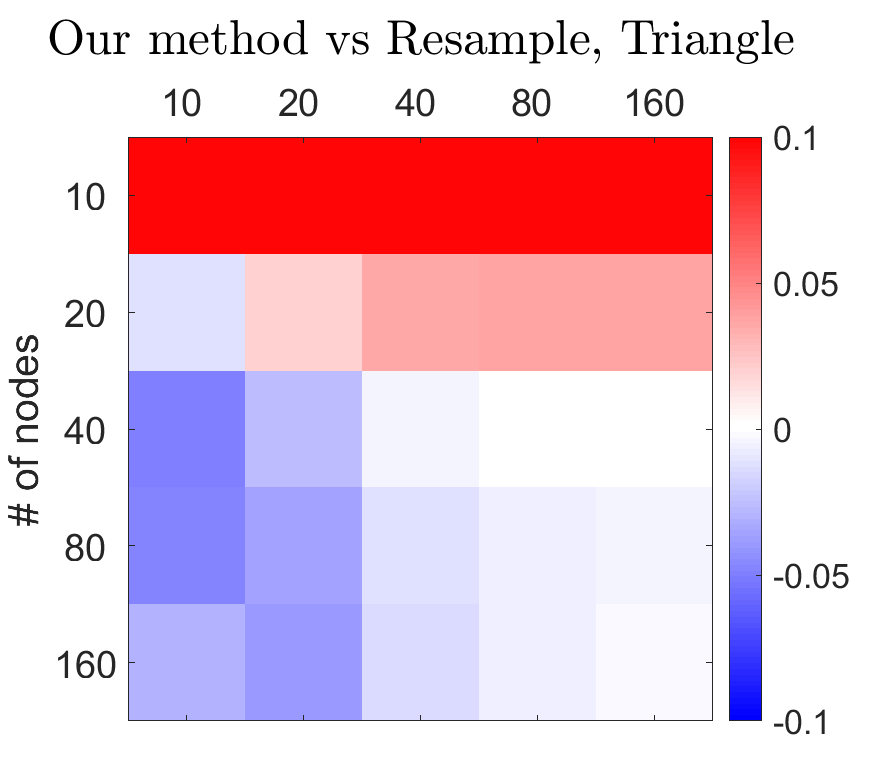
Figure 10 shows that our method controls coverage probabilities more accurately around the nominal level in most settings, except in the case where one network has only nodes. This is not surprising since the remainder terms ignored in the analytical approximation may be no longer ignorable when the network is very small. We recall that both node bootstrap methods in this simulation are also devised based on our formulation of . Node resampling shows good accuracy and robustness on some small network examples, but it is not scalable: it takes more than 12 hours to run node resampling experiments for settings. Due to page limit, we sink the numerical result tables to Section 12.1 in Supplementary Material.



12 Additional simulation set-up information and results
12.1 Addition simulation results for the simulation in Section 11.2 in Main Paper
Tables 2 – 9 show the numerical results of empirical 90% CI coverage probabilities of our method and approximation. The purpose of displaying these tables is to provide more details and confirm the marginal accuracy of our method, completing the message conveyed by Figure 10 in Main Paper.
Network sizes
Network sizes
Network sizes
Network sizes
Network sizes
Network sizes
Network sizes
Network sizes
12.2 Detailed simulation set-up information and full-X-range plots for Simulation 3 in Section 8.2 in Main Paper
In the simulation, we generated a large network database with 10 different graphon models, listed as follows. All these graphons’ functions have been rescaled such that . Set .
- 1.
SmoothGraphon-1: ;
- 2.
SmoothGraphon-2: , where ;
- 3.
SmoothGraphon-3: , where ;
- 4.
SmoothGraphon-4: , where ;
- 5.
SmoothGraphon-5: , where ; , where ;
- 6.
BlockModel-1: Stochastic block model with equal-sized communities and edge probabilities , where ;
- 7.
BlockModel-2: Stochastic block model with equal-sized communities and edge probabilities , where ;
- 8.
BlockModel-3: Stochastic block model with with sized communities and edge probabilities , where ;
- 9.
BlockModel-4: Stochastic block model with with sized communities and edge probabilities , where ;
- 10.
BlockModel-5: Stochastic block model with sized communities and edge probabilities , where .
The keyword network in the first experiment was generated from SmoothGraphon-1. The two keyword networks in the second experiment were generated from the following graphon models:
- •
Keyword 1: Same as BlockModel-1.
- •
Keyword 2: SmoothGraphon-6: , where .
Figure 11 shows full-X-range plots of Row 2 in Figure 2 in Main Paper, with two more cases , , both omitted in Main Paper to meet page limit. Particularly, the plot in Figure 11 better matches the interpretation at the end of the second paragraph in Section 8.2 in Main Paper, that there should be some cyan bars to the left of reference line, showing not-match.


12.3 Additional simulation results for Section 8.5


References
- Abbe (2017) Emmanuel Abbe. Community detection and stochastic block models: recent developments. The Journal of Machine Learning Research, 18(1):6446–6531, 2017.
- Adhikari et al. (2019) Bhim M Adhikari, L Elliot Hong, Hemalatha Sampath, Joshua Chiappelli, Neda Jahanshad, Paul M Thompson, Laura M Rowland, Vince D Calhoun, Xiaoming Du, and Shuo Chen. Functional network connectivity impairments and core cognitive deficits in schizophrenia. Human brain mapping, 40(16):4593–4605, 2019.
- Agterberg et al. (2020) Joshua Agterberg, Minh Tang, and Carey Priebe. Nonparametric two-sample hypothesis testing for random graphs with negative and repeated eigenvalues. arXiv preprint arXiv:2012.09828, 2020.
- Ahmed et al. (2015) Nesreen K Ahmed, Jennifer Neville, Ryan A Rossi, and Nick Duffield. Efficient graphlet counting for large networks. In 2015 IEEE International Conference on Data Mining, pages 1–10. IEEE, 2015.
- Arroyo et al. (2021) Jesús Arroyo, Daniel L Sussman, Carey E Priebe, and Vince Lyzinski. Maximum likelihood estimation and graph matching in errorfully observed networks. Journal of Computational and Graphical Statistics, 30(4):1111–1123, 2021.
- Banerjee and Ma (2017) Debapratim Banerjee and Zongming Ma. Optimal hypothesis testing for stochastic block models with growing degrees. arXiv preprint arXiv:1705.05305, 2017.
- Beran (1987) Rudolf Beran. Prepivoting to reduce level error of confidence sets. Biometrika, 74(3):457–468, 1987.
- Beran (1988) Rudolf Beran. Prepivoting test statistics: a bootstrap view of asymptotic refinements. Journal of the American Statistical Association, 83(403):687–697, 1988.
- Bhattacharya et al. (2022) Bhaswar B Bhattacharya, Sayan Das, and Sumit Mukherjee. Motif estimation via subgraph sampling: The fourth-moment phenomenon. The Annals of Statistics, 50(2):987–1011, 2022.
- Bhattacharyya and Bickel (2015) Sharmodeep Bhattacharyya and Peter J Bickel. Subsampling bootstrap of count features of networks. The Annals of Statistics, 43(6):2384–2411, 2015.
- Bickel and Chen (2009) Peter J Bickel and Aiyou Chen. A nonparametric view of network models and newman–girvan modularities. Proceedings of the National Academy of Sciences, 106(50):21068–21073, 2009.
- Bickel et al. (2011) Peter J Bickel, Aiyou Chen, and Elizaveta Levina. The method of moments and degree distributions for network models. The Annals of Statistics, 39(5):2280–2301, 2011.
- Bravo-Hermsdorff et al. (2021) Gecia Bravo-Hermsdorff, Lee M Gunderson, Pierre-André Maugis, and Carey E Priebe. A principled (and practical) test for network comparison. arXiv preprint arXiv:2107.11403, 2021.
- Chen et al. (2022) Andrew A Chen, Chongliang Luo, Yong Chen, Russell T Shinohara, Haochang Shou, Alzheimer’s Disease Neuroimaging Initiative, et al. Privacy-preserving harmonization via distributed combat. Neuroimage, 248:118822, 2022.
- Chen et al. (2022+) Li Chen, Nathaniel Josephs, Lizhen Lin, Jie Zhou, and Eric D Kolaczyk. A spectral-based framework for hypothesis testing in populations of networks. Statistica Sinica (In press), 2022+.
- Chen et al. (2022) Pindong Chen, Hongxiang Yao, Betty M Tijms, Pan Wang, Dawei Wang, Chengyuan Song, Hongwei Yang, Zengqiang Zhang, Kun Zhao, Yida Qu, et al. Four distinct subtypes of alzheimer’s disease based on resting-state connectivity biomarkers. Biological Psychiatry, 2022.
- Chen and Kato (2019) Xiaohui Chen and Kengo Kato. Randomized incomplete -statistics in high dimensions. The Annals of Statistics, 47(6):3127–3156, 2019.
- DasGupta (2008) Anirban DasGupta. Asymptotic theory of statistics and probability, volume 180. Springer, 2008.
- Decelle et al. (2011) Aurelien Decelle, Florent Krzakala, Cristopher Moore, and Lenka Zdeborová. Inference and phase transitions in the detection of modules in sparse networks. Physical Review Letters, 107(6):065701, 2011.
- Fan et al. (2012) Jianqing Fan, Xu Han, and Weijie Gu. Estimating false discovery proportion under arbitrary covariance dependence. Journal of the American Statistical Association, 107(499):1019–1035, 2012.
- Friguet et al. (2009) Chloé Friguet, Maela Kloareg, and David Causeur. A factor model approach to multiple testing under dependence. Journal of the American Statistical Association, pages 1406–1415, 2009.
- Gao and Lafferty (2017a) Chao Gao and John Lafferty. Testing network structure using relations between small subgraph probabilities. arXiv preprint arXiv:1704.06742, 2017a.
- Gao and Lafferty (2017b) Chao Gao and John Lafferty. Testing for global network structure using small subgraph statistics. arXiv preprint arXiv:1710.00862, 2017b.
- Gao et al. (2015) Chao Gao, Yu Lu, and Harrison H Zhou. Rate-optimal graphon estimation. The Annals of Statistics, 43(6):2624–2652, 2015.
- Gao et al. (2018) Chao Gao, Zongming Ma, Anderson Y Zhang, and Harrison H Zhou. Community detection in degree-corrected block models. Annals of Statistics, 46(5):2153–2185, 2018.
- Genovese and Wasserman (2002) Christopher Genovese and Larry Wasserman. Operating characteristics and extensions of the false discovery rate procedure. Journal of the Royal Statistical Society Series B: Statistical Methodology, 64(3):499–517, 2002.
- Ghoshdastidar and Von Luxburg (2018) Debarghya Ghoshdastidar and Ulrike Von Luxburg. Practical methods for graph two-sample testing. Advances in Neural Information Processing Systems, 31, 2018.
- Ghoshdastidar et al. (2017) Debarghya Ghoshdastidar, Maurilio Gutzeit, Alexandra Carpentier, and Ulrike von Luxburg. Two-sample tests for large random graphs using network statistics. In Conference on Learning Theory, pages 954–977. PMLR, 2017.
- Ghoshdastidar et al. (2020) Debarghya Ghoshdastidar, Maurilio Gutzeit, Alexandra Carpentier, and Ulrike Von Luxburg. Two-sample hypothesis testing for inhomogeneous random graphs. The Annals of Statistics, 48(4):2208–2229, 2020.
- Ginestet et al. (2017) Cedric E Ginestet, Jun Li, Prakash Balachandran, Steven Rosenberg, and Eric D Kolaczyk. Hypothesis testing for network data in functional neuroimaging. The Annals of Applied Statistics, pages 725–750, 2017.
- Green and Shalizi (2022) Alden Green and Cosma Rohilla Shalizi. Bootstrapping exchangeable random graphs. Electronic Journal of Statistics, 16(1):1058 – 1095, 2022. doi: 10.1214/21-EJS1896.
- Hall (2013) Peter Hall. The Bootstrap and Edgeworth Expansion. Springer Science & Business Media, 2013.
- Hall and Martin (1988) Peter Hall and Michael A Martin. On bootstrap resampling and iteration. Biometrika, 75(4):661–671, 1988.
- Hladky et al. (2021) Jan Hladky, Christos Pelekis, and Matas Sileikis. A limit theorem for small cliques in inhomogeneous random graphs. Journal of Graph Theory, 97(4):578–599, 2021.
- Hoeffding (1948) Wassily Hoeffding. A class of statistics with asymptotically normal distribution. The Annals of Mathematical Statistics, 19(3):293–325, 1948.
- Hunter et al. (2008) David R Hunter, Mark S Handcock, Carter T Butts, Steven M Goodreau, and Martina Morris. ergm: A package to fit, simulate and diagnose exponential-family models for networks. Journal of Statistical Software, 24(3), 2008.
- Jin et al. (2018) Jiashun Jin, Zheng Ke, and Shengming Luo. Network global testing by counting graphlets. In International Conference on Machine Learning, pages 2333–2341. PMLR, 2018.
- Kolaczyk et al. (2020) Eric D Kolaczyk, Lizhen Lin, Steven Rosenberg, Jackson Walters, and Jie Xu. Averages of unlabeled networks: Geometric characterization and asymptotic behavior. The Annals of Statistics, 48(1):514–538, 2020.
- Leskovec and Mcauley (2012) Jure Leskovec and Julian Mcauley. Learning to discover social circles in ego networks. Advances in Neural Information Processing Systems, 25, 2012.
- Levin and Levina (2019) Keith Levin and Elizaveta Levina. Bootstrapping networks with latent space structure. arXiv preprint arXiv:1907.10821, 2019.
- Li and Li (2018) Yezheng Li and Hongzhe Li. Two-sample test of community memberships of weighted stochastic block models. arXiv preprint arXiv:1811.12593, 2018.
- Lunde and Sarkar (2019) Robert Lunde and Purnamrita Sarkar. Subsampling sparse graphons under minimal assumptions. arXiv preprint arXiv:1907.12528, 2019.
- Lyzinski et al. (2015) Vince Lyzinski, Donniell E Fishkind, Marcelo Fiori, Joshua T Vogelstein, Carey E Priebe, and Guillermo Sapiro. Graph matching: Relax at your own risk. IEEE Transactions on Pattern Analysis and Machine Intelligence, 38(1):60–73, 2015.
- Maesono (1997) Yoshihiko Maesono. Edgeworth expansions of a studentized u-statistic and a jackknife estimator of variance. Journal of Statistical Planning and Inference, 61(1):61–84, 1997.
- Maugis et al. (2020) P-AG Maugis, SC Olhede, CE Priebe, and PJ Wolfe. Testing for equivalence of network distribution using subgraph counts. Journal of Computational and Graphical Statistics, 29(3):455–465, 2020.
- Maugis (2020) PA Maugis. Central limit theorems for local network statistics. arXiv preprint arXiv:2006.15738, 2020.
- Olhede and Wolfe (2014) Sofia C Olhede and Patrick J Wolfe. Network histograms and universality of blockmodel approximation. Proceedings of the National Academy of Sciences, 111(41):14722–14727, 2014.
- Sabanayagam et al. (2021) Mahalakshmi Sabanayagam, Leena Chennuru Vankadara, and Debarghya Ghoshdastidar. Graphon based clustering and testing of networks: Algorithms and theory. arXiv preprint arXiv:2110.02722, 2021.
- Serfling (2009) Robert J Serfling. Approximation theorems of mathematical statistics. John Wiley & Sons, 2009.
- Shao et al. (2023) Meijia Shao, Dong Xia, and Yuan Zhang. U-statistic reduction: Higher-order accurate risk control and statistical-computational trade-off, with application to network method-of-moments. arXiv preprint arXiv:2306.03793, 2023.
- Tang et al. (2017) Minh Tang, Avanti Athreya, Daniel L Sussman, Vince Lyzinski, Youngser Park, and Carey E Priebe. A semiparametric two-sample hypothesis testing problem for random graphs. Journal of Computational and Graphical Statistics, 26(2):344–354, 2017.
- Tsitsulin et al. (2018) Anton Tsitsulin, Davide Mottin, Panagiotis Karras, Alexander Bronstein, and Emmanuel Müller. Netlsd: hearing the shape of a graph. In Proceedings of the 24th ACM SIGKDD International Conference on Knowledge Discovery & Data Mining, pages 2347–2356, 2018.
- Wasserman (2006) Larry Wasserman. All of Nonparametric Statistics. Springer Science & Business Media, 2006.
- Wills and Meyer (2020) Peter Wills and François G Meyer. Metrics for graph comparison: a practitioner’s guide. Plos one, 15(2):e0228728, 2020.
- Yang et al. (2013) Jaewon Yang, Julian McAuley, and Jure Leskovec. Community detection in networks with node attributes. In 2013 IEEE 13th international conference on data mining, pages 1151–1156. IEEE, 2013.
- Yang et al. (2014) Justin Yang, Christina Han, and Edoardo Airoldi. Nonparametric estimation and testing of exchangeable graph models. In Artificial Intelligence and Statistics, pages 1060–1067. PMLR, 2014.
- Young and Scheinerman (2007) Stephen J Young and Edward R Scheinerman. Random dot product graph models for social networks. In International Workshop on Algorithms and Models for the Web-Graph, pages 138–149. Springer, 2007.
- Yuan and Wen (2021) Mingao Yuan and Qian Wen. A practical two-sample test for weighted random graphs. Journal of Applied Statistics, pages 1–17, 2021.
- Zhang and Xia (2022) Yuan Zhang and Dong Xia. Edgeworth expansions for network moments. The Annals of Statistics, 50(2):726–753, 2022.
- Zhang et al. (2017) Yuan Zhang, Elizaveta Levina, and Ji Zhu. Estimating network edge probabilities by neighbourhood smoothing. Biometrika, 104(4):771–783, 2017.
- Zhao (2023) Yufei Zhao. Graph Theory and Additive Combinatorics: Exploring Structure and Randomness. Cambridge University Press, 2023.