跳到论文正文
W Papers独立论文阅读器 arXiv:2208.07516 论文正文 计算阅读时间 · 0%
引用这篇论文根据当前论文元数据生成,正式投稿前建议核对。


License: CC BY 4.0
arXiv:2208.07516v1 [math.OC] 16 Aug 2022

An Optimal Control Problem with Terminal Stochastic Linear Complementarity ConstraintsThanks: Submitted to the editors DATE.

Jianfeng Luo Email: gstljf@polyu.edu.hk Thanks: CAS AMSS-PolyU Joint Laboratory of Applied Mathematics (Shenzhen), The Hong Kong Polytechnic University Shenzhen Research Institute, Shenzhen, China ().    Xiaojun Chen Email: maxjchen@polyu.edu.hk Thanks: Department of Applied Mathematics, The Hong Kong Polytechnic University, Hong Kong, China ().
Abstract

In this paper, we investigate an optimal control problem with terminal stochastic linear complementarity constraints (SLCC), and its discrete approximation using the relaxation, the sample average approximation (SAA) and the implicit Euler time-stepping scheme. We show the existence of feasible solutions and optimal solutions to the optimal control problem and its discrete approximation under the conditions that the expectation of the stochastic matrix in the SLCC is a Z-matrix or an adequate matrix. Moreover, we prove that the solution sequence generated by the discrete approximation converges to a solution of the original optimal control problem with probability 1 as ϵ↓0\epsilon\downarrow 0, ν→∞\nu\to\infty and h↓0h\downarrow 0, where ϵ\epsilon is the relaxation parameter, ν\nu is the sample size and hh is the mesh size. We also provide asymptotics of the SAA optimal value and error bounds of the time-stepping method. A numerical example is used to illustrate the existence of optimal solutions, the discretization scheme and error estimation.

keywords
linear complementarity problem, sample average approximation, implicit Euler time-stepping, convergence analysis, error estimate.
Funding.
This work is supported by the Hong Kong Research Grants Council grant PolyU15300021 and the CAS AMSS-PolyU Joint Laboratory in Applied Mathematics.
††runningheads: An Optimal Control Problem with Complementarity Constraints / J. LUO and X. CHEN
MSC
49M25, 49N10, 90C15, 90C33

1 Introduction

Let ξ\xi be a random variable defined in the probability space (Ω,ℱ,𝒫)(\Omega,\mathcal{F},\mathcal{P}) with support set Ξ:=ξ⁡(Ω)⊆ℝd\Xi:=\xi(\Omega)\subseteq\mathbb{R}^{d}. Let ∥⋅∥\|\cdot\| denote the Euclidean norm of a vector and a matrix. Let L2​(0,T)nL^{2}(0,T)^{n} denote the Banach space of all quadratically Lebesgue integrable functions mapping from (0,T)(0,T) to ℝn\mathbb{R}^{n}, which is equipped with the norm

‖x‖L2:=(∫0T‖x⁡(t)‖2​𝑑t)12,∀x∈L2​(0,T)n.\|x\|_{L^{2}}:=\left(\int_{0}^{T}\|x(t)\|^{2}dt\right)^{\frac{1}{2}},\,\,\,\forall\,\,x\in L^{2}(0,T)^{n}.

Denote H1​(0,T)nH^{1}(0,T)^{n} the space of all functions x∈L2​(0,T)nx\in L^{2}(0,T)^{n} whose components x1,⋯,xn:(0,T)→ℝx_{1},\cdot\cdot\cdot,x_{n}:(0,T)\rightarrow\mathbb{R} possess weak derivatives such that the function x˙∈L2​(0,T)n\dot{x}\in L^{2}(0,T)^{n}. A suitable norm in H1​(0,T)nH^{1}(0,T)^{n} is defined by

‖x‖H1:=(‖x‖L22+‖x˙‖L22)12,∀x∈H1​(0,T)n.\|x\|_{H^{1}}:=\left(\|x\|_{L^{2}}^{2}+\|\dot{x}\|_{L^{2}}^{2}\right)^{\frac{1}{2}},\,\,\,\forall\,\,x\in H^{1}(0,T)^{n}.

In this paper, we aim to find an optimal solution (x,u)∈H1​(0,T)n×L2​(0,T)m(x,u)\in H^{1}(0,T)^{n}\times L^{2}(0,T)^{m} of the following optimal control problem with terminal stochastic linear complementarity constraints:

minx,u⁡Φ⁡(x,u):=𝔼⁡[F⁡(x⁡(T),ξ)]+12​‖x−xd‖L22+δ2​‖u−ud‖L22\displaystyle\min_{x,u}\,\,\Phi(x,u):=\mathbb{E}[F(x(T),\xi)]+\frac{1}{2}\|x-x_{d}\|_{L^{2}}^{2}+\frac{\delta}{2}\|u-u_{d}\|_{L^{2}}^{2} (1)
s.t.{x˙​(t)=A​x​(t)+B​u​(t),C​x​(t)+D​u​(t)−f⁡(t)≤0,}a.e.t∈(0,T),0≤x⁡(T)⟂𝔼⁡[M⁡(ξ)​x​(T)+q⁡(ξ)]≥0,x(0)=x0,𝔼[g(x(T),ξ)]∈K,\displaystyle\textrm{s.t.}\left\{\begin{aligned} &\left.\begin{aligned} &\dot{x}(t)=Ax(t)+Bu(t),&\\ &Cx(t)+Du(t)-f(t)\leq 0,&\\ \end{aligned}\right\}a.e.\,\,t\in(0,T),&\\ &0\leq x(T)\perp\mathbb{E}[M(\xi)x(T)+q(\xi)]\geq 0,&\\ &x(0)=x_{0},\,\mathbb{E}[g(x(T),\xi)]\in K,\end{aligned}\right.

where A∈ℝn×nA\in\mathbb{R}^{n\times n}, B∈ℝn×mB\in\mathbb{R}^{n\times m}, C∈ℝl×nC\in\mathbb{R}^{l\times n}, D∈ℝl×mD\in\mathbb{R}^{l\times m}, x0∈ℝnx_{0}\in\mathbb{R}^{n} and f∈L2​(0,T)lf\in L^{2}(0,T)^{l} are given, δ>0\delta>0 is a scalar, K⊆ℝℓK\subseteq\mathbb{R}^{\ell} is a nonempty, closed and convex set. Here xd∈L2​(0,T)nx_{d}\in L^{2}(0,T)^{n} and ud∈L2​(0,T)mu_{d}\in L^{2}(0,T)^{m} are the given desired state and control, respectively. The mappings F:ℝn×Ξ→ℝF:\mathbb{R}^{n}\times\Xi\rightarrow\mathbb{R} and g:ℝn×Ξ→ℝℓg:\mathbb{R}^{n}\times\Xi\rightarrow\mathbb{R}^{\ell} are continuously differentiable over ℝn\mathbb{R}^{n} for almost every ξ∈Ξ\xi\in\Xi, and are measurable on Ξ\Xi for each z∈ℝnz\in\mathbb{R}^{n}. Two mappings M:Ξ→ℝn×nM:\Xi\rightarrow\mathbb{R}^{n\times n} and q:Ξ→ℝnq:\Xi\rightarrow\mathbb{R}^{n} are also measurable in ξ∈Ξ\xi\in\Xi.

In [2], Benita and Mehlita studied an optimal control problem with terminal deterministic complementarity constraints, which has many interesting practical applications in multi-agent control networks. They derived some stationarity conditions and presented constraint qualifications which ensure that these conditions hold at a local optimal solution of the optimal control problem under the assumption that the feasible set is nonempty. However, sufficient conditions were not given for the existence of x⁡(T)x(T) such that the terminal deterministic complementarity constraints

0≤x⁡(T)⟂M¯​x​(T)+q¯≥0,\displaystyle 0\leq x(T)\perp\bar{M}x(T)+\bar{q}\geq 0, (2)
g¯​(x​(T))∈K,\displaystyle\bar{g}(x(T))\in K, (3)

hold, where M¯∈ℝn×n\bar{M}\in\mathbb{R}^{n\times n}, q¯∈ℝn\bar{q}\in\mathbb{R}^{n} and g¯:ℝn→ℝℓ\bar{g}:\mathbb{R}^{n}\rightarrow\mathbb{R}^{\ell}. Problem (1) extends the problem in [2] to terminal stochastic case in uncertain environment.

Optimal control with differential equations and complementarity constraints provides a powerful modeling paradigm for many practical problems such as the optimal control of electrical networks with diodes and/or MOS transistors [4] and dynamic optimization of chemical processes [22]. It can also be derived from the KKT conditions of a bilevel optimal control if the lower level problem is convex and satisfies a constraint qualification [17]. A series of works [5, 6, 10, 14, 24] are devoted to the study of optimal control problems with complementarity constraints. It should be noted that these papers focus on deterministic problems, where the system coefficients including system parameters and boundary/initial conditions are perfectly known. On the other hand, optimal control problems with stochastic differential equation constraints under uncertain environment have been extensively studied [16, 19, 20]. These papers investigate theory and algorithms for optimal control when the parameters in the differential equations have noise and uncertainties. However, there is very little research on optimal control with terminal stochastic complementarity constraints.

The main contributions of this paper are summarized as follows. We show the existence of feasible solutions to the optimal control problem (1) under the conditions that 𝔼⁡[M⁡(ξ)]\mathbb{E}[M(\xi)] is a Z-matrix or an adequate matrix, which gives reasonable conditions for the existence of x⁡(T)x(T) such that (2)-(3) hold. Moreover, we prove the existence of feasible solutions and optimal solutions to the discrete approximation using the relaxation, the sample average approximation (SAA) and the implicit Euler time-stepping scheme under the same conditions. In the convergence analysis, we prove that the solution sequence generated by the discrete approximation converges to a solution of the original optimal control problem with probability 1 (w.p.1) as ϵ↓0\epsilon\downarrow 0, ν→∞\nu\to\infty and h↓0h\downarrow 0, where ϵ\epsilon is the relaxation parameter, ν\nu is the sample size and hh is the mesh size. We also provide asymptotics of the SAA optimal value and error bounds of the time-stepping method. These results extend the approximation error of the Euler time-stepping method of an optimal control problem with convex terminal constraints to nonconvex terminal stochastic complementarity constraints.

The paper is organised as follows: Section 2 deals with the existence of feasible solutions of problem (1). Section 3 studies the existence of feasible solutions of the relaxation and the SAA of (1) and the convergence to the original problem (1) as the relaxation parameter goes to zero and the sample size approaches to infinity. In Section 4, we study the convergence of the time-stepping scheme and show the convergence properties of the discrete method using the SAA and the implicit Euler time-stepping scheme. A numerical example is given in Section 5 to illustrate the theoretical results obtained in this paper. Final conclusion remarks are presented in Section 6.

1.1 Notation and assumptions

Throughout this paper we use the following notation. For a matrix A∈ℝm×nA\in\mathbb{R}^{m\times n}, Ai∙A_{i\bullet} and A∙jA_{\bullet j} denote its iith row and jjth column, respectively, A⊤A^{\top} denotes its transpose matrix, and A†A^{\dagger} is its pseudoinverse matrix. If AA possesses full row rank mm, we have A†=A⊤​(A​A⊤)−1A^{\dagger}=A^{\top}(AA^{\top})^{-1}. Let II denote the identity matrix with a certain dimension.

For sets S1,S2⊆ℝn{S}_{1},S_{2}\subseteq\mathbb{R}^{n}, we denote the distance from v∈ℝnv\in\mathbb{R}^{n} to S1S_{1} and the deviation of the set S1S_{1} from the set S2S_{2} by dist​(v,S1)=infv′∈S1‖v−v′‖,\textrm{dist}(v,S_{1})=\inf_{v^{\prime}\in S_{1}}\|v-v^{\prime}\|, and 𝔻⁡(S1,S2)=supv∈S1dist​(v,S2)\mathbb{D}(S_{1},S_{2})=\sup_{v\in S_{1}}\textrm{dist}(v,S_{2}), respectively. For sets S1,S2⊆H1​(0,T)n×L2​(0,T)m{S}_{1},S_{2}\subseteq H^{1}(0,T)^{n}\times L^{2}(0,T)^{m}, we denote the distance from (v1,v2)∈H1​(0,T)n×L2​(0,T)m(v_{1},v_{2})\in H^{1}(0,T)^{n}\times L^{2}(0,T)^{m} to S1S_{1} by dist​((v1,v2),S1)=inf(v1′,v2′)∈S1(‖v1−v1′‖H1+‖v2−v2′‖L2),\textrm{dist}((v_{1},v_{2}),S_{1})=\inf_{(v^{\prime}_{1},v^{\prime}_{2})\in S_{1}}(\|v_{1}-v^{\prime}_{1}\|_{H^{1}}+\|v_{2}-v^{\prime}_{2}\|_{L^{2}}), and the deviation of the set S1S_{1} from the set S2S_{2} by 𝔻⁡(S1,S2)=sup(v1,v2)∈S1dist​((v1,v2),S2)\mathbb{D}(S_{1},S_{2})=\sup_{(v_{1},v_{2})\in S_{1}}\textrm{dist}((v_{1},v_{2}),S_{2}). Let ℬ⁡(v,ε)={w:‖w−v‖≤ε}\mathcal{B}(v,\varepsilon)=\{w:\|w-v\|\leq\varepsilon\} be the closed ball centered at vv with the radius of ε\varepsilon. Let intSS denote the interior of a set SS. Let [N]={1,2,…,N}.[N]=\{1,2,\ldots,N\}.

We give two basic assumptions to ensure that problem (1) is well defined.

Assumption 1.

There exist four nonnegative measurable functions κi​(ξ)\kappa_{i}(\xi) with 𝔼​[κi​(ξ)]<∞\mathbb{E}[\kappa_{i}(\xi)]<\infty (i=1,2,3,4)(i=1,2,3,4) such that for any z1z_{1}, z2∈ℝnz_{2}\in\mathbb{R}^{n},

|F(z1,ξ)−F(z2,ξ)|≤κ1(ξ)∥z1−z2∥,∥g(z1,ξ)∥≤κ2(ξ)∥z1∥,a.e.ξ∈Ξ,|F(z_{1},\xi)-F(z_{2},\xi)|\leq\kappa_{1}(\xi)\|z_{1}-z_{2}\|,\,\,\|g(z_{1},\xi)\|\leq\kappa_{2}(\xi)\|z_{1}\|,\,\,a.e.\,\,\xi\in\Xi,

and

‖M⁡(ξ)‖≤κ3​(ξ)​and​‖q⁡(ξ)‖≤κ4​(ξ),∀ξ∈Ξ.\|M(\xi)\|\leq\kappa_{3}(\xi)\,\,\,\textrm{and}\,\,\,\|q(\xi)\|\leq\kappa_{4}(\xi),\,\,\,\forall\,\,\xi\in\Xi.

Assumption 2.

The matrix D∈ℝl×mD\in\mathbb{R}^{l\times m} is full row rank with l<ml<m and the matrix

ℛ:=[BY(A−BD†C)BY(A−BD†C)2BY⋯(A−BD†C)n−1BY]∈ℝn×n⁡(m−l)\mathcal{R}:=[BY\,\,\,\,(A-BD^{\dagger}C)BY\,\,\,(A-BD^{\dagger}C)^{2}BY\,\,\,\cdot\cdot\cdot\,\,\,(A-BD^{\dagger}C)^{n-1}BY]\in\mathbb{R}^{n\times n(m-l)}

is also full row rank, where Y∈ℝm×(m−l)Y\in\mathbb{R}^{m\times(m-l)} is a matrix with full column rank m−lm-l such that D​Y=0DY=0.

2 Existence of optimal solutions of problem (1)

In this section, we first investigate the feasibility of problem (1). We call (x,u)∈H1​(0,T)n×L2​(0,T)m(x,u)\in H^{1}(0,T)^{n}\times L^{2}(0,T)^{m} a feasible solution of (1) if it satisfies the constraints in (1).

For an index set J⊆{1,2,⋯,n}J\subseteq\{1,2,\cdot\cdot\cdot,n\}, let |J||J| denote its cardinality and JcJ^{c} denote its complementarity set. We denote by qJ∈ℝ|J|q_{J}\in\mathbb{R}^{|J|} the subvector formed from a vector q∈ℝnq\in\mathbb{R}^{n} by picking the entries indexed by JJ and denote by MJ1,J2∈ℝ|J1|×|J2|M_{J_{1},J_{2}}\in\mathbb{R}^{|J_{1}|\times|J_{2}|} the submatrix formed from a matrix M∈ℝn×nM\in\mathbb{R}^{n\times n} by picking the rows indexed by J1J_{1} and columns indexed by J2J_{2}. Let 𝒥={J:𝔼[MJ,J(ξ)]{\cal J}=\{J\,:\,\mathbb{E}[M_{J,J}(\xi)] is nonsingular}\} and

β={1if​𝒥=∅,max⁡{‖(𝔼⁡[MJ,J​(ξ)])−1‖1|J∈𝒥}otherwise.\beta=\left\{\begin{array}[]{ll}1&{\rm if}\,{\cal J}=\emptyset,\\ \max\{\|(\mathbb{E}[M_{J,J}(\xi)])^{-1}\|_{1}\,\,|\,\,J\in{\cal J}\}&{\rm otherwise.}\end{array}\right.

A square matrix is said to be a P-matrix if all its principal minors are positive. A square matrix is said to be a Z-matrix if its off-diagonal entries are non-positive. A matrix 𝔼⁡[M⁡(ξ)]∈ℝn×n\mathbb{E}[M(\xi)]\in\mathbb{R}^{n\times n} is called column adequate if for each z∈ℝnz\in\mathbb{R}^{n}, zi​(𝔼⁡[M⁡(ξ)]​z)i≤0z_{i}(\mathbb{E}[M(\xi)]z)_{i}\leq 0 for all i=1,2,⋯,ni=1,2,\cdot\cdot\cdot,n implies 𝔼⁡[M⁡(ξ)]​z=0\mathbb{E}[M(\xi)]z=0. The matrix 𝔼⁡[M⁡(ξ)]\mathbb{E}[M(\xi)] is row adequate if 𝔼​[M⁡(ξ)]⊤\mathbb{E}[M(\xi)]^{\top} is column adequate and it is adequate if it is both column and row adequate [11]. It is known that a P-matrix is adequate and a symmetric positive semi-definite matrix is also adequate [11, Theorem 3.1.7, Theorem 3.4.4]. However, an adequate matrix may neither be a P-matrix nor a positive semi-definite matrix [11].

Theorem 3.

Let Assumption 1 and Assumption 2 hold. Suppose the following three conditions hold: (i) ℬ⁡(0,β​𝔼​[κ2​(ξ)]​‖𝔼⁡[q⁡(ξ)]‖1)⊆K\mathcal{B}(0,\beta\mathbb{E}[\kappa_{2}(\xi)]\|\mathbb{E}[q(\xi)]\|_{1})\subseteq K, (ii) the set

𝒱:={v∈ℝn|𝔼[M(ξ)v+q(ξ)]≥0,v≥0}\mathcal{V}:=\{v\in\mathbb{R}^{n}\,|\,\mathbb{E}[M(\xi)v+q(\xi)]\geq 0,\,v\geq 0\}

is nonempty, and (iii) 𝔼⁡[M⁡(ξ)]\mathbb{E}[M(\xi)] is an adequate matrix or a Z-matrix. Then problem (1) has a feasible solution (x,u)∈H1​(0,T)n×L2​(0,T)m(x,u)\in H^{1}(0,T)^{n}\times L^{2}(0,T)^{m}. Moreover, the optimal control problem (1) admits an optimal solution if 𝔼⁡[F⁡(⋅,ξ)]\mathbb{E}[F(\cdot,\xi)] is bounded from below.

Proof.

Following Lemma 7.2 in [2], Assumption 2 implies that the following system

{x˙​(t)=A​x​(t)+B​u​(t),C​x​(t)+D​u​(t)=p⁡(t),x(0)=x0,x(T)=b,a.e.t∈(0,T),\left\{\begin{aligned} &\dot{x}(t)=Ax(t)+Bu(t),&\\ &Cx(t)+Du(t)=p(t),&\\ &x(0)=x_{0},\,\,\,x(T)=b,&\\ \end{aligned}\right.\,\,a.e.\,\,t\in(0,T), (4)

admits a solution (x,u)∈H1​(0,T)n×L2​(0,T)m(x,u)\in H^{1}(0,T)^{n}\times L^{2}(0,T)^{m} for any p∈L2​(0,T)lp\in L^{2}(0,T)^{l} and b∈ℝnb\in\mathbb{R}^{n}. If we set p​(t)=f​(t)+p~​(t)p(t)=f(t)+\tilde{p}(t) in (4) for arbitrary p~∈L2​(0,T)l\tilde{p}\in L^{2}(0,T)^{l} with p~​(t)≤0\tilde{p}(t)\leq 0 and f⁡(t)f(t) in (1), then the following problem

{x˙​(t)=A​x​(t)+B​u​(t),C​x​(t)+D​u​(t)−f⁡(t)≤0,x(0)=x0,x(T)=b,a.e.t∈(0,T),\left\{\begin{aligned} &\dot{x}(t)=Ax(t)+Bu(t),&\\ &Cx(t)+Du(t)-f(t)\leq 0,&\\ &x(0)=x_{0},\,\,\,x(T)=b,&\\ \end{aligned}\right.\,\,a.e.\,\,t\in(0,T), (5)

has a solution (x,u)∈H1​(0,T)n×L2​(0,T)m(x,u)\in H^{1}(0,T)^{n}\times L^{2}(0,T)^{m} for any b∈ℝnb\in\mathbb{R}^{n}.

Now we show the solution set of the following stochastic constrained LCP is nonempty,

{min⁡{x⁡(T),𝔼⁡[M⁡(ξ)​x​(T)+q⁡(ξ)]}=0,𝔼⁡[g⁡(x⁡(T),ξ)]∈K.\left\{\begin{aligned} &\min\{x(T),\,\mathbb{E}[M(\xi)x(T)+q(\xi)]\}=0,&\\ &\mathbb{E}[g(x(T),\xi)]\in K.\end{aligned}\right. (6)

Following Corollary 3.3.5 and Theorem 3.11.6 in [11], the LCP in (6) has a solution from the assumption that the set 𝒱\mathcal{V} is nonempty and 𝔼⁡[M⁡(ξ)]\mathbb{E}[M(\xi)] is adequate or a Z-matrix. Let x∗​(T)x^{*}(T) be a sparse solution of the LCP in (6), which is defined as

x∗​(T)∈\displaystyle x^{*}(T)\in argmin​‖x⁡(T)‖0\displaystyle\rm{\displaystyle argmin}\,\|x(T)\|_{0}
s.t.0≤x⁡(T)⟂𝔼⁡[M⁡(ξ)​x​(T)+q⁡(ξ)]≥0,\displaystyle\rm{\displaystyle s.t.}\quad\quad 0\leq x(T)\perp\mathbb{E}[M(\xi)x(T)+q(\xi)]\geq 0,

where ‖x⁡(T)‖0=\|x(T)\|_{0}= the number of nonzero components of x⁡(T)x(T). If there is no JJ such that 𝔼​[MJ,J​(ξ)]\mathbb{E}[M_{J,J}(\xi)] is nonsingular, that is, 𝒥=∅{\cal J}=\emptyset, then by Theorem 2.2 in [8] and Theorem 3.1 in [9], ‖x∗​(T)‖0=‖x∗​(T)‖1=0.\|x^{*}(T)\|_{0}=\|x^{*}(T)\|_{1}=0. Hence, we have

‖x∗​(T)‖≤β​‖𝔼⁡[q⁡(ξ)]‖1.\|x^{*}(T)\|\leq\beta\|\mathbb{E}[q(\xi)]\|_{1}. (7)

If there is JJ such that x∗​(T)J>0x^{*}(T)_{J}>0 and x∗​(T)Jc=0x^{*}(T)_{J^{c}}=0, from Theorem 2.2 in [8] and Theorem 3.1 in [9], we know that 𝔼​[MJ,J​(ξ)]\mathbb{E}[M_{J,J}(\xi)] is nonsingular and

x∗​(T)=−(I−Λ+Λ​𝔼​[M⁡(ξ)])−1​Λ​𝔼​[q⁡(ξ)],x^{*}(T)=-(I-\Lambda+\Lambda\mathbb{E}[M(\xi)])^{-1}\Lambda\mathbb{E}[q(\xi)],

where Λ\Lambda is a diagonal matrix with Λi,i=1,\Lambda_{i,i}=1, if i∈Ji\in J and Λi,i=0,\Lambda_{i,i}=0, if i∈Jci\in J^{c}. Moreover, from

‖(I−Λ+Λ​𝔼​[M⁡(ξ)])−1​Λ‖≤max⁡{‖(𝔼⁡[MJ,J​(ξ)])−1‖1|J∈𝒥},\|(I-\Lambda+\Lambda\mathbb{E}[M(\xi)])^{-1}\Lambda\|\leq\max\{\|(\mathbb{E}[M_{J,J}(\xi)])^{-1}\|_{1}\,|\,J\in{\cal J}\},

we obtain (7) for 𝒥≠∅{\cal J}\neq\emptyset.

Therefore, from Assumption 1 and assumption (i) of this theorem, we have

‖𝔼⁡[g⁡(x∗​(T),ξ)]‖≤𝔼⁡[κ2​(ξ)]​‖x∗​(T)‖≤𝔼⁡[κ2​(ξ)]​‖x∗​(T)‖1≤β​𝔼​[κ2​(ξ)]​‖𝔼⁡[q⁡(ξ)]‖1,\displaystyle\|\mathbb{E}[g(x^{*}(T),\xi)]\|\leq\mathbb{E}[\kappa_{2}(\xi)]\|x^{*}(T)\|\leq\mathbb{E}[\kappa_{2}(\xi)]\|x^{*}(T)\|_{1}\leq\beta\mathbb{E}[\kappa_{2}(\xi)]\|\mathbb{E}[q(\xi)]\|_{1},

which implies that 𝔼⁡[g⁡(x∗​(T),ξ)]∈K\mathbb{E}[g(x^{*}(T),\xi)]\in K. Hence the solution set of (6) is nonempty.

Similar to the proof of Theorem 5.1 in [2], we can derive the existence of optimal solutions to problem (1) under the assumption that 𝔼⁡[F⁡(⋅,ξ)]\mathbb{E}[F(\cdot,\xi)] is bounded from below.

Remark 4.

The constrained LCP (6) may have multiple solutions or may not have a solution. If 𝔼⁡[M⁡(ξ)]\mathbb{E}[M(\xi)] is a P-matrix, then for any 𝔼⁡[q⁡(ξ)]\mathbb{E}[q(\xi)], the LCP in (6) has a unique solution x⁡(T)x(T). In such case, if 𝔼⁡[g⁡(x⁡(T),ξ)]∈K\mathbb{E}[g(x(T),\xi)]\in K, then (6) has a unique solution, otherwise (6) does not have a solution. If 𝔼⁡[M⁡(ξ)]\mathbb{E}[M(\xi)] is a Z-matrix or an adequate matrix, the LCP in (6) may have multiple solutions, while some solutions can be bounded by β​‖𝔼⁡[q⁡(ξ)]‖1\beta\|\mathbb{E}[q(\xi)]\|_{1}. When ℬ⁡(0,β​𝔼​[κ2​(ξ)]​‖𝔼⁡[q⁡(ξ)]‖1)\mathcal{B}(0,\beta\mathbb{E}[\kappa_{2}(\xi)]\|\mathbb{E}[q(\xi)]\|_{1}) ⊆K\subseteq K, some solutions of the LCP satisfy 𝔼⁡[g⁡(x⁡(T),ξ)]∈K\mathbb{E}[g(x(T),\xi)]\in K and thus the constrained LCP (6) is solvable. See the example in Section 5.

Remark 5.

Assumption 2 is also used in [2] for the case l<ml<m, which allows more freedom for the system controls. If l=ml=m and DD is invertible, we can write C​x​(t)+D​u​(t)−f⁡(t)=−v⁡(t)Cx(t)+Du(t)-f(t)=-v(t) with v⁡(t)≥0v(t)\geq 0 for a.e. t∈[0,T]t\in[0,T], where v∈L2​(0,T)lv\in L^{2}(0,T)^{l}. Then the solvability of (5) becomes to find a solution pair (x,v)∈H1​(0,T)n×L2​(0,T)l(x,v)\in H^{1}(0,T)^{n}\times L^{2}(0,T)^{l} with v⁡(t)≥0v(t)\geq 0 satisfying

{x˙​(t)=(A−B​D−1​C)​x​(t)+B​D−1​f​(t)−B​D−1​v​(t),x(0)=x0,x(T)=b,a.e.t∈(0,T).\left\{\begin{aligned} &\dot{x}(t)=(A-BD^{-1}C)x(t)+BD^{-1}f(t)-BD^{-1}v(t),&\\ &x(0)=x_{0},\,\,\,x(T)=b,&\\ \end{aligned}\right.\,\,a.e.\,\,t\in(0,T). (8)

It then requires the concept of positive controllability [3, 25]. Therefore, the conditions to ensure the solution set of (8) is nonempty for any b∈ℝnb\in\mathbb{R}^{n} are (i) the matrix

[BD−1(A−BD−1C)BD−1(A−BD−1C)2BD−1⋯(A−BD−1C)n−1BD−1][BD^{-1}\,\,\,\,(A-BD^{-1}C)BD^{-1}\,\,\,(A-BD^{-1}C)^{2}BD^{-1}\,\,\,\cdot\cdot\cdot\,\,\,(A-BD^{-1}C)^{n-1}BD^{-1}]

possesses full row rank nn, and (ii) there is no real eigenvector w∈ℝn\textbf{w}\in\mathbb{R}^{n} of (A−B​D−1​C)⊤(A-BD^{-1}C)^{\top} such that w⊤​B​D−1​v≥0\textbf{w}^{\top}BD^{-1}\textbf{v}\geq 0 for any v∈ℝ+m\textbf{v}\in\mathbb{R}^{m}_{+}. Then there is a finite time T0T_{0} such that the solution set of (5) is nonempty for any b∈ℝnb\in\mathbb{R}^{n} and T≥T0T\geq T_{0}. Hence we can replace Assumption 2 in Theorem 3 by these two conditions for the case that l=ml=m and DD is invertible.

3 Relaxation and sample average approximation (SAA)

In this section, we apply the relaxation and the SAA approach to solve (1). We consider an independent identically distributed (i.i.d) sample of ξ⁡(ω)\xi(\omega), which is denoted by {ξ1,⋯,ξν}\{\xi_{1},\cdot\cdot\cdot,\xi_{\nu}\}, and use the following relaxation and SAA problem to approximate problem (1):

minx,u⁡Φν​(x,u):=1ν​∑ℓ=1νF⁡(x⁡(T),ξℓ)+12​‖x−xd‖L22+δ2​‖u−ud‖L22\displaystyle\min_{x,u}\,\,\Phi^{\nu}(x,u):=\frac{1}{\nu}\sum_{\ell=1}^{\nu}F(x(T),\xi_{\ell})+\frac{1}{2}\|x-x_{d}\|_{L^{2}}^{2}+\frac{\delta}{2}\|u-u_{d}\|_{L^{2}}^{2} (9)
s.t.{x˙​(t)=A​x​(t)+B​u​(t),C​x​(t)+D​u​(t)−f⁡(t)≤0,}a.e.t∈(0,T),‖min⁡{x⁡(T),1ν​∑ℓ=1ν[M⁡(ξℓ)​x​(T)+q⁡(ξℓ)]}‖≤ϵ,x(0)=x0,1ν∑ℓ=1νg(x(T),ξℓ)∈Kϵ:={z|dist(z,K)≤ϵ},\displaystyle\textrm{s.t.}\left\{\begin{aligned} &\left.\begin{aligned} &\dot{x}(t)=Ax(t)+Bu(t),&\\ &Cx(t)+Du(t)-f(t)\leq 0,\end{aligned}\right\}a.e.\,\,t\in(0,T),&\\ &\left\|\min\left\{x(T),\frac{1}{\nu}\sum_{\ell=1}^{\nu}[M(\xi_{\ell})x(T)+q(\xi_{\ell})]\right\}\right\|\leq\epsilon,&\\ &x(0)=x_{0},\,\,\,\frac{1}{\nu}\sum_{\ell=1}^{\nu}g(x(T),\xi_{\ell})\in K^{\epsilon}:=\left\{z\,|\,{\rm dist}(z,K)\leq\epsilon\right\},\end{aligned}\right.

where ϵ>0\epsilon>0 is a sufficiently small number.

3.1 Convergence of the relaxation and SAA

In this subsection, we show the existence of a solution of problem (9), and its convergence as ϵ↓0\epsilon\downarrow 0 and ν→∞\nu\to\infty.

Theorem 6.

Suppose that the conditions in Theorem 3 hold. Then for any ϵ>0\epsilon>0, the SAA problem (9) has an optimal solution (xϵ,ν,uϵ,ν)∈H1​(0,T)n×L2​(0,T)m(x^{\epsilon,\nu},u^{\epsilon,\nu})\in H^{1}(0,T)^{n}\times L^{2}(0,T)^{m} for sufficiently large ν\nu w.p.1.

Proof.

Since the solution set of the linear control system (5) is nonempty for any b∈ℝnb\in\mathbb{R}^{n}, for the existence of a feasible solution to the SAA problem (9), it suffices to show the solution set of the following system

{‖min⁡{x⁡(T),1ν​∑ℓ=1ν[M⁡(ξℓ)​x​(T)+q⁡(ξℓ)]}‖≤ϵ,1ν​∑ℓ=1νg⁡(x⁡(T),ξℓ)∈Kϵ\left\{\begin{aligned} &\left\|\min\left\{x(T),\frac{1}{\nu}\sum_{\ell=1}^{\nu}[M(\xi_{\ell})x(T)+q(\xi_{\ell})]\right\}\right\|\leq\epsilon,&\\ &\frac{1}{\nu}\sum_{\ell=1}^{\nu}g(x(T),\xi_{\ell})\in K^{\epsilon}\end{aligned}\right. (10)

is nonempty w.p.1 for any positive number ϵ\epsilon.

Let x∗​(T)x^{*}(T) be a sparse solution of the LCP in (6). From Theorem 3, we know that x∗​(T)x^{*}(T) satisfies (6). By the Law of Large Number, for sufficiently lager ν\nu, x∗​(T)x^{*}(T) is a solution of (10). It concludes that the solution set of the system (10) is nonempty w.p.1 for sufficiently large ν\nu.

Since 𝔼⁡[F⁡(⋅,ξ)]\mathbb{E}[F(\cdot,\xi)] is bounded from below, we can also obtain that 1ν​∑ℓ=1νF⁡(⋅,ξℓ)\frac{1}{\nu}\sum_{\ell=1}^{\nu}F(\cdot,\xi_{\ell}) is bounded from below with sufficiently large ν\nu. The existence of optimal solutions to problem (9) is similar to the proof of Theorem 3.

Since F⁡(⋅,ξ)F(\cdot,\xi) is a smoothing function for a.e. ξ∈Ξ\xi\in\Xi, following the proof of Lemma 3.5 in [7], we can have the following lemma.

Lemma 7.

Let 𝒞1×𝒞2\mathcal{C}_{1}\times\mathcal{C}_{2} denote a compact subset of H1​(0,T)n×L2​(0,T)mH^{1}(0,T)^{n}\times L^{2}(0,T)^{m}. It holds that Φν\Phi^{\nu} epiconverges to Φ\Phi w.p.1 over 𝒞1×𝒞2\mathcal{C}_{1}\times\mathcal{C}_{2} as ν→∞\nu\rightarrow\infty.

Let 𝒵ϵ,ν\mathcal{Z}^{\epsilon,\nu} and 𝒵\mathcal{Z} denote the solution sets of (10) and (6), respectively. Let 𝒮ϵ,ν\mathcal{S}^{\epsilon,\nu} and 𝒮\mathcal{S} be the feasible solution sets, and 𝒮^ϵ,ν\hat{\mathcal{S}}^{\epsilon,\nu} and 𝒮^\hat{\mathcal{S}} be optimal solution sets of (9) and (1), respectively.

Theorem 8.

Suppose that the conditions of Theorem 3 hold, then it holds that limϵ↓0limν→∞𝔻⁡(𝒵ϵ,ν,𝒵)=0\lim_{\epsilon\downarrow 0}\lim_{\nu\rightarrow\infty}\mathbb{D}(\mathcal{Z}^{\epsilon,\nu},\mathcal{Z})=0 w.p.1, limϵ↓0limν→∞𝔻⁡(𝒮ϵ,ν,𝒮)=0\lim_{\epsilon\downarrow 0}\lim_{\nu\rightarrow\infty}\mathbb{D}(\mathcal{S}^{\epsilon,\nu},\mathcal{S})=0 w.p.1. and limϵ↓0limν→∞𝔻⁡(𝒮^ϵ,ν,𝒮^)=0\lim_{\epsilon\downarrow 0}\lim_{\nu\rightarrow\infty}\mathbb{D}(\hat{\mathcal{S}}^{\epsilon,\nu},\hat{\mathcal{S}})=0 w.p.1.

Proof.

From Theorem 3 and Theorem 6, 𝒵\mathcal{Z} and 𝒵ϵ,ν\mathcal{Z}^{\epsilon,\nu} with any ϵ>0\epsilon>0 and large enough ν\nu are nonempty. By (7) and ℬ⁡(0,β​𝔼​[κ2​(ξ)]​‖𝔼⁡[q⁡(ξ)]‖1)⊆K\mathcal{B}(0,\beta\mathbb{E}[\kappa_{2}(\xi)]\|\mathbb{E}[q(\xi)]\|_{1})\subseteq K in Theorem 3, we know that there is a compact set 𝒳\mathcal{X} such that 𝒵⊆𝒳\mathcal{Z}\subseteq\mathcal{X} and 𝒵ϵ,ν⊆𝒳\mathcal{Z}^{\epsilon,\nu}\subseteq\mathcal{X} for sufficiently small ϵ\epsilon and sufficiently large ν\nu. Let

ϕ(x(T)):=min{x(T),𝔼[M(ξ)x(T)+q(ξ)]}andψ(x(T)):=𝔼[g(x(T),ξ)].\phi(x(T)):=\min\{x(T),\mathbb{E}[M(\xi)x(T)+q(\xi)]\}\quad{\rm and}\quad\psi(x(T)):=\mathbb{E}[g(x(T),\xi)].

For x⁡(T)∈𝒵x(T)\in\mathcal{Z}, ϕ⁡(x⁡(T))=0\phi(x(T))=0 and ψ⁡(x⁡(T))∈K.\psi(x(T))\in K. From (10), for x⁡(T)∈𝒵ϵ,νx(T)\in\mathcal{Z}^{\epsilon,\nu}, there are vν∈ℝn,wν∈ℝℓv^{\nu}\in\mathbb{R}^{n},w^{\nu}\in\mathbb{R}^{\ell} with ‖vν‖≤ϵ\|v^{\nu}\|\leq\epsilon and ‖wν‖≤ϵ\|w^{\nu}\|\leq\epsilon such that

ϕϵν​(x⁡(T)):=min⁡{x⁡(T),1ν​∑ℓ=1ν[M⁡(ξℓ)​x​(T)+q⁡(ξℓ)]}+vν=0,\displaystyle\phi^{\nu}_{\epsilon}(x(T)):=\min\left\{x(T),\frac{1}{\nu}\sum_{\ell=1}^{\nu}[M(\xi_{\ell})x(T)+q(\xi_{\ell})]\right\}+v^{\nu}=0,
ψϵν​(x⁡(T)):=1ν​∑ℓ=1νg⁡(x⁡(T),ξℓ)+wν∈K.\displaystyle\psi^{\nu}_{\epsilon}(x(T)):=\frac{1}{\nu}\sum_{\ell=1}^{\nu}g(x(T),\xi_{\ell})+w^{\nu}\in K.

Since ϕ\phi and ψ\psi are continuous, and M⁡(⋅),q⁡(⋅)M(\cdot),q(\cdot) and g⁡(x⁡(T),⋅)g(x(T),\cdot) satisfy Assumption 1, we have ϕϵν\phi^{\nu}_{\epsilon} and ψϵν\psi^{\nu}_{\epsilon} converge to ϕ\phi and ψ\psi uniformly, respectively on the compact set 𝒳\mathcal{X}, that is,

limϵ↓0limν→∞maxx⁡(T)∈𝒳⁡‖ϕϵν​(x⁡(T))−ϕ⁡(x⁡(T))‖=0,\lim_{\epsilon\downarrow 0}\lim_{\nu\to\infty}\max_{x(T)\in\mathcal{X}}\|\phi^{\nu}_{\epsilon}(x(T))-\phi(x(T))\|=0,

and

limϵ↓0limν→∞maxx⁡(T)∈𝒳⁡‖ψϵν​(x⁡(T))−ψ⁡(x⁡(T))‖=0.\lim_{\epsilon\downarrow 0}\lim_{\nu\to\infty}\max_{x(T)\in\mathcal{X}}\|\psi^{\nu}_{\epsilon}(x(T))-\psi(x(T))\|=0.

Therefore, following Theorem 5.12 in [23], limϵ↓0limν→∞𝔻⁡(𝒵ϵ,ν,𝒵)=0\lim_{\epsilon\downarrow 0}\lim_{\nu\rightarrow\infty}\mathbb{D}(\mathcal{Z}^{\epsilon,\nu},\mathcal{Z})=0 w.p.1.

Now we show limϵ↓0limν→∞𝔻⁡(𝒮ϵ,ν,𝒮)=0\lim_{\epsilon\downarrow 0}\lim_{\nu\rightarrow\infty}\mathbb{D}(\mathcal{S}^{\epsilon,\nu},\mathcal{S})=0 holds w.p.1. Note that 𝒮ϵ,ν\mathcal{S}^{\epsilon,\nu} and 𝒮\mathcal{S} are two nonempty closed sets. Obviously, two nonempty closed sets 𝒮\mathcal{S} and 𝒮ϵ,ν\mathcal{S}^{\epsilon,\nu} are the solution sets of problem (5) with terminal sets 𝒵\mathcal{Z} and 𝒵ϵ,ν\mathcal{Z}^{\epsilon,\nu}, respectively. For any p∈L2​(0,T)lp\in L^{2}(0,T)^{l}, the pair (‖x‖H1,‖u‖L2)(\|x\|_{H^{1}},\|u\|_{L^{2}}), where (x,u)(x,u) is a solution of problem (4), is uniquely defined by the terminal point x⁡(T)x(T). In addition, it is clear that a solution (x,u)(x,u) of problem (4) is continuous with respect to the terminal point x⁡(T)x(T). Hence, for any (xϵ,ν,uϵ,ν)∈𝒮ϵ,ν(x^{\epsilon,\nu},u^{\epsilon,\nu})\in\mathcal{S}^{\epsilon,\nu} and (x,u)∈𝒮(x,u)\in\mathcal{S}, we have (xϵ,ν,uϵ,ν)→(x,u)(x^{\epsilon,\nu},u^{\epsilon,\nu})\rightarrow(x,u) w.p.1 in the norm ∥⋅∥H1×∥⋅∥L2\|\cdot\|_{H^{1}}\times\|\cdot\|_{L^{2}} when xϵ,ν​(T)→x​(T)x^{\epsilon,\nu}(T)\rightarrow x(T) w.p.1 as ϵ↓0\epsilon\downarrow 0 and ν→∞\nu\rightarrow\infty. It then concludes limϵ↓0limν→∞𝔻⁡(𝒮ϵ,ν,𝒮)=0\lim_{\epsilon\downarrow 0}\lim_{\nu\rightarrow\infty}\mathbb{D}(\mathcal{S}^{\epsilon,\nu},\mathcal{S})=0 w.p.1.

It is clear that, arg⁡min⁡Φ=𝒮^⊆𝒮\arg\min\Phi=\hat{\mathcal{S}}\subseteq\mathcal{S} and arg⁡min⁡Φν=𝒮^ϵ,ν⊆𝒮ϵ,ν\arg\min\Phi^{\nu}=\hat{\mathcal{S}}^{\epsilon,\nu}\subseteq\mathcal{S}^{\epsilon,\nu} for sufficiently small ϵ\epsilon and sufficiently large ν\nu. By limϵ↓0limν→∞𝔻⁡(𝒮ϵ,ν,𝒮)=0\lim_{\epsilon\downarrow 0}\lim_{\nu\rightarrow\infty}\mathbb{D}(\mathcal{S}^{\epsilon,\nu},\mathcal{S})=0 w.p.1, we have, for (x^ϵ,ν,u^ϵ,ν)∈𝒮^ϵ,ν(\hat{x}^{\epsilon,\nu},\hat{u}^{\epsilon,\nu})\in\hat{\mathcal{S}}^{\epsilon,\nu}, there is (x^,u^)∈𝒮(\hat{x},\hat{u})\in\mathcal{S} such that (x^ϵ,ν,u^ϵ,ν)→(x^,u^)(\hat{x}^{\epsilon,\nu},\hat{u}^{\epsilon,\nu})\rightarrow(\hat{x},\hat{u}) in the norm ∥⋅∥H1×∥⋅∥L2\|\cdot\|_{H^{1}}\times\|\cdot\|_{L^{2}} as ϵ↓0\epsilon\downarrow 0 and ν→∞\nu\rightarrow\infty. In addition, according to Theorem 2.5 in [1], we obtain (x^,u^)∈𝒮^(\hat{x},\hat{u})\in\hat{\mathcal{S}} by Φν→e​p​iΦ\Phi^{\nu}\xrightarrow{epi}\Phi w.p.1, which implies limϵ↓0limν→∞𝔻⁡(𝒮^ϵ,ν,𝒮^)=0\lim_{\epsilon\downarrow 0}\lim_{\nu\rightarrow\infty}\mathbb{D}(\hat{\mathcal{S}}^{\epsilon,\nu},\hat{\mathcal{S}})=0 w.p.1.

3.2 Asymptotics of the SAA optimal value

We introduce the relaxation of problem (1) with a parameter ϵ>0\epsilon>0 as follows

minx,u⁡Φ⁡(x,u)\displaystyle\min_{x,u}\,\,\Phi(x,u) (11)
s.t.{x˙​(t)=A​x​(t)+B​u​(t),C​x​(t)+D​u​(t)−f⁡(t)≤0,}a.e.t∈(0,T),‖min⁡{x⁡(T),𝔼⁡[M⁡(ξ)​x​(T)+q⁡(ξ)]}‖≤ϵ,x(0)=x0,𝔼[g(x(T),ξ)]∈Kϵ.\displaystyle\textrm{s.t.}\left\{\begin{aligned} &\left.\begin{aligned} &\dot{x}(t)=Ax(t)+Bu(t),&\\ &Cx(t)+Du(t)-f(t)\leq 0,&\\ \end{aligned}\right\}a.e.\,\,t\in(0,T),&\\ &\|\min\{x(T),\mathbb{E}[M(\xi)x(T)+q(\xi)]\}\|\leq\epsilon,&\\ &x(0)=x_{0},\,\mathbb{E}[g(x(T),\xi)]\in K^{\epsilon}.\end{aligned}\right.

Denote by 𝒵ϵ\mathcal{Z}^{\epsilon} the solution set of the terminal constraints of (11). Denote by 𝒮ϵ\mathcal{S}^{\epsilon} and 𝒮^ϵ\hat{\mathcal{S}}^{\epsilon} the feasible solution set and optimal solution set of (11), respectively. Recall that 𝒵\mathcal{Z} is the solution set of (6), and 𝒮\mathcal{S} and 𝒮^\hat{\mathcal{S}} are the feasible solution set and optimal solution set of (1), respectively. It is clear that 𝒵⊆𝒵ϵ\mathcal{Z}\subseteq\mathcal{Z}^{\epsilon} and 𝒮⊆𝒮ϵ\mathcal{S}\subseteq\mathcal{S}^{\epsilon}, which mean that Φ⁡(x^ϵ,u^ϵ)≤Φ⁡(x^,u^)\Phi(\hat{x}^{\epsilon},\hat{u}^{\epsilon})\leq\Phi(\hat{x},\hat{u}) for any (x^ϵ,u^ϵ)∈𝒮^ϵ(\hat{x}^{\epsilon},\hat{u}^{\epsilon})\in\hat{\mathcal{S}}^{\epsilon} and (x^,u^)∈𝒮^(\hat{x},\hat{u})\in\hat{\mathcal{S}}. Therefore, 𝒵ϵ\mathcal{Z}^{\epsilon}, 𝒮ϵ\mathcal{S}^{\epsilon} and 𝒮^ϵ\hat{\mathcal{S}}^{\epsilon} are nonempty since 𝒵\mathcal{Z} and 𝒮\mathcal{S} are nonempty.

According to Theorem 3 and Remark 4, we also conclude that 𝒵ϵ\mathcal{Z}^{\epsilon} and 𝒮^ϵ\hat{\mathcal{S}}^{\epsilon} are compact. It can also be derived that limϵ↓0𝔻⁡(𝒵ϵ,𝒵)=0\lim_{\epsilon\downarrow 0}\mathbb{D}(\mathcal{Z}^{\epsilon},\mathcal{Z})=0, limϵ↓0𝔻⁡(𝒮ϵ,𝒮)=0\lim_{\epsilon\downarrow 0}\mathbb{D}(\mathcal{S}^{\epsilon},\mathcal{S})=0 and limϵ↓0𝔻⁡(𝒮^ϵ,𝒮^)=0\lim_{\epsilon\downarrow 0}\mathbb{D}(\hat{\mathcal{S}}^{\epsilon},\hat{\mathcal{S}})=0. It is clear that (9) is the corresponding SAA problem of (11). By Theorem 8, we conclude that limν→∞𝔻⁡(𝒵ϵ,ν,𝒵ϵ)=0\lim_{\nu\rightarrow\infty}\mathbb{D}({\mathcal{Z}}^{\epsilon,\nu},{\mathcal{Z}}^{\epsilon})=0, limν→∞𝔻⁡(𝒮ϵ,ν,𝒮ϵ)=0\lim_{\nu\rightarrow\infty}\mathbb{D}({\mathcal{S}}^{\epsilon,\nu},{\mathcal{S}}^{\epsilon})=0 and limν→∞𝔻⁡(𝒮^ϵ,ν,𝒮^ϵ)=0\lim_{\nu\rightarrow\infty}\mathbb{D}(\hat{\mathcal{S}}^{\epsilon,\nu},\hat{\mathcal{S}}^{\epsilon})=0.

In the rest of this section, we study the asymptotics of optimal value of the SAA problem (9) for a fixed ϵ>0\epsilon>0.

Since min⁡{x⁡(T),𝔼⁡[M⁡(ξ)​x​(T)+q⁡(ξ)]}=0\min\{x(T),\mathbb{E}[M(\xi)x(T)+q(\xi)]\}=0 and 𝔼⁡[g⁡(x⁡(T),ξ)]∈K\mathbb{E}[g(x(T),\xi)]\in K for any x⁡(T)∈𝒵x(T)\in\mathcal{Z}, we have 𝒵⊆int​𝒵ϵ\mathcal{Z}\subseteq\textrm{int}\mathcal{Z}^{\epsilon}, which means that int​𝒵ϵ≠∅\textrm{int}\mathcal{Z}^{\epsilon}\neq\emptyset. Let

𝒵^={x⁡(T):(x,u)∈𝒮^}and𝒵^ϵ={x⁡(T):(x,u)∈𝒮^ϵ}.\hat{\mathcal{Z}}=\{x(T):\,(x,u)\in\hat{\mathcal{S}}\}\quad{\rm and}\quad\hat{\mathcal{Z}}^{\epsilon}=\{x(T):\,(x,u)\in\hat{\mathcal{S}}^{\epsilon}\}.

Obviously, we have 𝒵^⊆int​𝒵ϵ\hat{\mathcal{Z}}\subseteq\textrm{int}\mathcal{Z}^{\epsilon} and limϵ↓0𝔻⁡(𝒵^ϵ,𝒵^)=0\lim_{\epsilon\downarrow 0}\mathbb{D}(\hat{\mathcal{Z}}^{\epsilon},\hat{\mathcal{Z}})=0.

We give the following assumptions.

Assumption 9.

The set 𝒵^\hat{\mathcal{Z}} is a singleton.

Assumption 10.
  • (i)

    There exists a nonnegative measurable function κ1​(ξ)\kappa_{1}(\xi) with 𝔼⁡[κ12​(ξ)]<∞\mathbb{E}[\kappa_{1}^{2}(\xi)]<\infty such that for any z1z_{1}, z2∈ℝnz_{2}\in\mathbb{R}^{n} and ξ∈Ξ\xi\in\Xi,

    |F⁡(z1,ξ)−F⁡(z2,ξ)|≤κ1​(ξ)​‖z1−z2‖,|F(z_{1},\xi)-F(z_{2},\xi)|\leq\kappa_{1}(\xi)\|z_{1}-z_{2}\|,

    and 𝔼⁡[F2​(z,ξ)]<∞\mathbb{E}[F^{2}(z,\xi)]<\infty for any z∈ℝnz\in\mathbb{R}^{n}.

  • (ii)

    The function 𝔼⁡[F⁡(⋅,ξ)]\mathbb{E}[F(\cdot,\xi)] is a strongly convex function, that is, there is a constant μ>0\mu>0 such that, for any z1z_{1}, z2∈ℝnz_{2}\in\mathbb{R}^{n} and τ∈(0,1)\tau\in(0,1),

    𝔼⁡[F⁡((1−τ)​z1+τ​z2,ξ)]≤(1−τ)​𝔼​[F⁡(z1,ξ)]+τ​𝔼​[F⁡(z2,ξ)]−μ​τ​(1−τ)2​‖z1−z2‖2.\displaystyle\hskip-21.68121pt\mathbb{E}[F((1-\tau)z_{1}+\tau z_{2},\xi)]\leq(1-\tau)\mathbb{E}[F(z_{1},\xi)]+\tau\mathbb{E}[F(z_{2},\xi)]-\frac{\mu\tau(1-\tau)}{2}\|z_{1}-z_{2}\|^{2}.

Theorem 11.

Suppose that the conditions of Theorem 3, Assumption 9 and Assumption 10 hold. Let (x^ϵ,u^ϵ)(\hat{x}^{\epsilon},\hat{u}^{\epsilon}) and (x^ϵ,ν,u^ϵ,ν)(\hat{x}^{\epsilon,\nu},\hat{u}^{\epsilon,\nu}) be optimal solutions of (11) and (9), respectively. Then for sufficiently small ϵ\epsilon and sufficiently large ν\nu, we have

ν​(Φν​(x^ϵ,ν,u^ϵ,ν)−Φ⁡(x^ϵ,u^ϵ))→𝐷𝒩⁡(0,σ2​(x^ϵ​(T))),\sqrt{\nu}(\Phi^{\nu}(\hat{x}^{\epsilon,\nu},\hat{u}^{\epsilon,\nu})-\Phi(\hat{x}^{\epsilon},\hat{u}^{\epsilon}))\quad\xrightarrow{D}\quad\mathcal{N}(0,\sigma^{2}(\hat{x}^{\epsilon}(T))),

where “ →𝐷\xrightarrow{D} ” denotes convergence in distribution and 𝒩⁡(0,σ2​(x^ϵ​(T)))\mathcal{N}(0,\sigma^{2}(\hat{x}^{\epsilon}(T))) denotes the norm distribution with mean 0 and variance σ2​(x^ϵ​(T)):=𝕍​ar​[F⁡(x^ϵ​(T),ξ)]\sigma^{2}(\hat{x}^{\epsilon}(T)):=\mathbb{V}\textrm{ar}[F(\hat{x}^{\epsilon}(T),\xi)].

Proof.

Since 𝒵^\hat{\mathcal{Z}} is a singleton, 𝒵^⊆int​𝒵ϵ\hat{\mathcal{Z}}\subseteq\textrm{int}\mathcal{Z}^{\epsilon} and limϵ↓0𝔻⁡(𝒵^ϵ,𝒵^)=0\lim_{\epsilon\downarrow 0}\mathbb{D}(\hat{\mathcal{Z}}^{\epsilon},\hat{\mathcal{Z}})=0, we have 𝒵^ϵ⊆int​𝒵ϵ\hat{\mathcal{Z}}^{\epsilon}\subseteq\textrm{int}\mathcal{Z}^{\epsilon} for sufficiently small ϵ\epsilon, which means that there is a convex set 𝒵𝒳\mathcal{Z}_{\mathcal{X}} such that 𝒵^ϵ⊆𝒵𝒳⊆𝒵ϵ\hat{\mathcal{Z}}^{\epsilon}\subseteq\mathcal{Z}_{\mathcal{X}}\subseteq\mathcal{Z}^{\epsilon} for sufficiently small ϵ\epsilon. We can also obtain that 𝒵^ϵ\hat{\mathcal{Z}}^{\epsilon} is a singleton for sufficiently small ϵ\epsilon under Assumption 10(ii). We argue it by contradiction. Suppose (x^ϵ,u^ϵ)(\hat{x}^{\epsilon},\hat{u}^{\epsilon}) and (xˇϵ,uˇϵ)(\check{x}^{\epsilon},\check{u}^{\epsilon}) are two optimal solutions of (11) with x^ϵ​(T)≠xˇϵ​(T)\hat{x}^{\epsilon}(T)\neq\check{x}^{\epsilon}(T). Then (xτϵ,uτϵ):=((1−τ)​x^ϵ+τ​xˇϵ,(1−τ)​u^ϵ+τ​uˇϵ)(x^{\epsilon}_{\tau},u^{\epsilon}_{\tau}):=((1-\tau)\hat{x}^{\epsilon}+\tau\check{x}^{\epsilon},(1-\tau)\hat{u}^{\epsilon}+\tau\check{u}^{\epsilon}) with τ∈(0,1)\tau\in(0,1) is also a feasible solution of (11), since xτϵ​(T)∈𝒵𝒳⊆𝒵ϵx^{\epsilon}_{\tau}(T)\in\mathcal{Z}_{\mathcal{X}}\subseteq\mathcal{Z}^{\epsilon}. Moreover,

Φ⁡(xτϵ,uτϵ)≤(1−τ)​Φ​(x^ϵ,u^ϵ)+τ​Φ​(xˇϵ,uˇϵ)−μ​τ​(1−τ)2​‖x^ϵ​(T)−xˇϵ​(T)‖2,\displaystyle\Phi(x^{\epsilon}_{\tau},u^{\epsilon}_{\tau})\leq(1-\tau)\Phi(\hat{x}^{\epsilon},\hat{u}^{\epsilon})+\tau\Phi(\check{x}^{\epsilon},\check{u}^{\epsilon})-\frac{\mu\tau(1-\tau)}{2}\|\hat{x}^{\epsilon}(T)-\check{x}^{\epsilon}(T)\|^{2},

which means Φ⁡(xτϵ,uτϵ)<Φ⁡(x^ϵ,u^ϵ)\Phi(x^{\epsilon}_{\tau},u^{\epsilon}_{\tau})<\Phi(\hat{x}^{\epsilon},\hat{u}^{\epsilon}) since Φ⁡(x^ϵ,u^ϵ)=Φ⁡(xˇϵ,uˇϵ)\Phi(\hat{x}^{\epsilon},\hat{u}^{\epsilon})=\Phi(\check{x}^{\epsilon},\check{u}^{\epsilon}) and x^ϵ​(T)≠xˇϵ​(T)\hat{x}^{\epsilon}(T)\neq\check{x}^{\epsilon}(T). It contradicts the assumption that (x^ϵ,u^ϵ)(\hat{x}^{\epsilon},\hat{u}^{\epsilon}) is an optimal solution of (11), and then we know that 𝒵^ϵ\hat{\mathcal{Z}}^{\epsilon} is a singleton for sufficiently small ϵ\epsilon.

In the following argument, ϵ>0\epsilon>0 is a fixed number such that 𝒵^ϵ\hat{\mathcal{Z}}^{\epsilon} is singleton and 𝒵^ϵ⊆int​𝒵ϵ\hat{\mathcal{Z}}^{\epsilon}\subseteq\textrm{int}{\mathcal{Z}}^{\epsilon}. Denote 𝒵^ϵ,ν={x⁡(T):(x,u)∈𝒮^ϵ,ν}\hat{\mathcal{Z}}^{\epsilon,\nu}=\{x(T):\,(x,u)\in\hat{\mathcal{S}}^{\epsilon,\nu}\}. We then obtain that limν→∞𝔻⁡(𝒵^ϵ,ν,𝒵^ϵ)=0\lim_{\nu\rightarrow\infty}\mathbb{D}(\hat{\mathcal{Z}}^{\epsilon,\nu},\hat{\mathcal{Z}}^{\epsilon})=0 and 𝒵^ϵ⊆int​𝒵ϵ,ν\hat{\mathcal{Z}}^{\epsilon}\subseteq\textrm{int}\mathcal{Z}^{\epsilon,\nu} for sufficiently large ν\nu according to limν→∞𝔻⁡(𝒵ϵ,ν,𝒵ϵ)=0\lim_{\nu\rightarrow\infty}\mathbb{D}({\mathcal{Z}}^{\epsilon,\nu},{\mathcal{Z}}^{\epsilon})=0. Therefore, there is a (x^ϵ,ν,u^ϵ,ν)∈𝒮^ϵ,ν(\hat{x}^{\epsilon,\nu},\hat{u}^{\epsilon,\nu})\in\hat{\mathcal{S}}^{\epsilon,\nu} such that x^ϵ,ν​(T)∈int​𝒵ϵ,ν\hat{x}^{\epsilon,\nu}(T)\in\textrm{int}\mathcal{Z}^{\epsilon,\nu} with sufficiently large ν\nu, which implies that, for sufficiently large ν\nu, there is a compact set 𝒳\mathcal{X} such that 𝒵^ϵ⊆𝒳⊆𝒵ϵ\hat{\mathcal{Z}}^{\epsilon}\subseteq\mathcal{X}\subseteq\mathcal{Z}^{\epsilon} and x^ϵ,ν​(T)∈𝒳⊆𝒵ϵ,ν\hat{x}^{\epsilon,\nu}(T)\in\mathcal{X}\subseteq\mathcal{Z}^{\epsilon,\nu}.

The solution (x,u)(x,u) of ODE (5) is continuous with respect to the state terminal value x⁡(T)x(T) and the pair (‖x‖H1,‖u‖L2)(\|x\|_{H^{1}},\|u\|_{L^{2}}) is uniquely defined by x⁡(T)x(T). Therefore, there is a compact set 𝔛\mathfrak{X} such that 𝒮^ϵ⊆𝔛⊆𝒮ϵ\hat{\mathcal{S}}^{\epsilon}\subseteq\mathfrak{X}\subseteq{\mathcal{S}}^{\epsilon} and 𝔛⊆𝒮ϵ,ν\mathfrak{X}\subseteq{\mathcal{S}}^{\epsilon,\nu} with 𝒮^ϵ,ν∩𝔛≠∅\hat{\mathcal{S}}^{\epsilon,\nu}\cap\mathfrak{X}\neq\emptyset. To derive the error of approximation for optimal value of (9) to that of (11), it suffices to investigate the error approximation for optimal value of the following problem

min(x,u)∈𝔛⁡Φ⁡(x,u)\displaystyle\min_{(x,u)\in\mathfrak{X}}\Phi(x,u) (12)

and its SAA problem

min(x,u)∈𝔛⁡Φν​(x,u),\displaystyle\min_{(x,u)\in\mathfrak{X}}\Phi^{\nu}(x,u), (13)

where Φ\Phi and Φν\Phi^{\nu} are defined in (11) and (9), respectively. Clearly, 𝔛⊆𝒮ϵ\mathfrak{X}\subseteq{\mathcal{S}}^{\epsilon} with 𝒮^ϵ∩𝔛≠∅\hat{\mathcal{S}}^{\epsilon}\cap\mathfrak{X}\neq\emptyset and 𝔛⊆𝒮ϵ,ν\mathfrak{X}\subseteq{\mathcal{S}}^{\epsilon,\nu} with 𝒮^ϵ,ν∩𝔛≠∅\hat{\mathcal{S}}^{\epsilon,\nu}\cap\mathfrak{X}\neq\emptyset mean that an optimal solution of (12) is an optimal solution of (11), and an optimal solution of (13) is also an optimal solution of (9). Therefore, according to Theorem 5.7 in [23], we can obtain that, under Assumption 10,

ν​(Φν​(x^ϵ,ν,u^ϵ,ν)−Φ⁡(x^ϵ,u^ϵ))\displaystyle\sqrt{\nu}(\Phi^{\nu}(\hat{x}^{\epsilon,\nu},\hat{u}^{\epsilon,\nu})-\Phi(\hat{x}^{\epsilon},\hat{u}^{\epsilon}))
=ν​(1ν​∑ℓ=1νF⁡(x^ϵ,ν​(T),ξℓ)+12​‖x^ϵ,ν−xd‖L22+δ2​‖u^ϵ,ν−ud‖L22CLOSE\displaystyle=\sqrt{\nu}(\frac{1}{\nu}\sum_{\ell=1}^{\nu}F(\hat{x}^{\epsilon,\nu}(T),\xi_{\ell})+\frac{1}{2}\|\hat{x}^{\epsilon,\nu}-x_{d}\|_{L^{2}}^{2}+\frac{\delta}{2}\|\hat{u}^{\epsilon,\nu}-u_{d}\|_{L^{2}}^{2}
OPEN−𝔼⁡[F⁡(x^ϵ​(T),ξ)]−12​‖x^ϵ−xd‖L22−δ2​‖u^ϵ−ud‖L22)\displaystyle\quad\quad\quad-\mathbb{E}[F(\hat{x}^{\epsilon}(T),\xi)]-\frac{1}{2}\|\hat{x}^{\epsilon}-x_{d}\|_{L^{2}}^{2}-\frac{\delta}{2}\|\hat{u}^{\epsilon}-u_{d}\|_{L^{2}}^{2})
→𝐷inf(x,u)∈𝒮^ϵY⁡(x,u),\displaystyle\xrightarrow{D}\inf_{(x,u)\in\hat{\mathcal{S}}^{\epsilon}}Y(x,u),

where Y⁡(x,u)Y(x,u) has a normal distribution with mean 0 and variance 𝕍​ar​[F⁡(x⁡(T),ξ)]\mathbb{V}\textrm{ar}[F(x(T),\xi)] with (x,u)∈𝒮^ϵ(x,u)\in\hat{\mathcal{S}}^{\epsilon}. Since 𝒵^ϵ={x^ϵ​(T)}\hat{\mathcal{Z}}^{\epsilon}=\{\hat{x}^{\epsilon}(T)\} is a singleton, Y⁡(x,u)Y(x,u) for any (x,u)∈𝒮^ϵ(x,u)\in\hat{\mathcal{S}}^{\epsilon} has the same normal distribution with mean 0 and variance 𝕍​ar​[F⁡(x^ϵ​(T),ξ)]\mathbb{V}\textrm{ar}[F(\hat{x}^{\epsilon}(T),\xi)]. It then concludes our desired result.

4 The time-stepping method

We now adopt the time-stepping method for solving problem (9) with a fixed sample {ξ1,…,ξν}\{\xi_{1},\ldots,\xi_{\nu}\}, which uses a finite-difference formula to approximate the time derivative x˙\dot{x}. It begins with the division of the time interval [0,T][0,T] into NN subintervals for a fixed step size h=T/N=ti+1−tih={T}/{N}=t_{i+1}-t_{i} where i=0,⋯,N−1i=0,\cdot\cdot\cdot,N-1. Starting from 𝐱0ν=x0\mathbf{x}_{0}^{\nu}=x_{0}, we compute two finite sets of vectors {𝐱1ϵ,ν,𝐱2ϵ,ν,⋯,𝐱Nϵ,ν}⊂ℝn\{\mathbf{x}^{\epsilon,\nu}_{1},\mathbf{x}^{\epsilon,\nu}_{2},\cdot\cdot\cdot,\mathbf{x}^{\epsilon,\nu}_{N}\}\subset\mathbb{R}^{n} and {𝐮1ϵ,ν,𝐮2ϵ,ν,⋯,𝐮Nϵ,ν}⊂ℝm\{\mathbf{u}^{\epsilon,\nu}_{1},\mathbf{u}^{\epsilon,\nu}_{2},\cdot\cdot\cdot,\mathbf{u}^{\epsilon,\nu}_{N}\}\subset\mathbb{R}^{m} in the following manner:

min{𝐱i,𝐮i}i=1N⁡1ν​∑ℓ=1νF⁡(𝐱N,ξℓ)+h2​∑i=1N(‖𝐱i−xd,i‖2+δ​‖𝐮i−ud,i‖2)\displaystyle\min_{\{\mathbf{x}_{i},\mathbf{u}_{i}\}_{i=1}^{N}}\,\,\frac{1}{\nu}\sum_{\ell=1}^{\nu}F(\mathbf{x}_{N},\xi_{\ell})+\frac{h}{2}\sum_{i=1}^{N}\left(\|\mathbf{x}_{i}-x_{d,i}\|^{2}+{\delta}\|\mathbf{u}_{i}-u_{d,i}\|^{2}\right) (14)
s.t.{𝐱i+1−𝐱i=h​A​𝐱i+1+h​B​𝐮i+1,C​𝐱i+1+D​𝐮i+1−fi+1≤0,}i=0,1,⋯,N−1,‖min⁡{𝐱N,1ν​∑ℓ=1ν[M⁡(ξℓ)​𝐱N+q⁡(ξℓ)]}‖≤ϵ,1ν​∑ℓ=1νg⁡(𝐱N,ξℓ)∈Kϵ,\displaystyle\textrm{s.t.}\left\{\begin{aligned} &\left.\begin{aligned} &\mathbf{x}_{i+1}-\mathbf{x}_{i}=hA\mathbf{x}_{i+1}+hB\mathbf{u}_{i+1},&\\ &C\mathbf{x}_{i+1}+D\mathbf{u}_{i+1}-f_{i+1}\leq 0,\end{aligned}\right\}i=0,1,\cdot\cdot\cdot,N-1,&\\ &\left\|\min\left\{\mathbf{x}_{N},\frac{1}{\nu}\sum_{\ell=1}^{\nu}[M(\xi_{\ell})\mathbf{x}_{N}+q(\xi_{\ell})]\right\}\right\|\leq\epsilon,&\\ &\frac{1}{\nu}\sum_{\ell=1}^{\nu}g(\mathbf{x}_{N},\xi_{\ell})\in K^{\epsilon},\end{aligned}\right.

where ϵ>0\epsilon>0 is a sufficiently small number, xd,i=xd​(ti)x_{d,i}=x_{d}(t_{i}), ud,i=ud​(ti)u_{d,i}=u_{d}(t_{i}) and fi=f⁡(ti)f_{i}=f(t_{i}) for i∈[N]i\in[N].

Theorem 12.

Suppose that the conditions of Theorem 3 hold, then for any ϵ>0\epsilon>0, problem (14) has an optimal solution for sufficiently large ν\nu and sufficiently small hh w.p.1.

Proof.

Theorem 6 has shown that the solution set of (10) with any ϵ>0\epsilon>0 is nonempty for sufficiently large ν\nu w.p.1. About the existence of feasible solution to problem (14), it suffices to show that the following problem has a solution for any b∈ℝnb\in\mathbb{R}^{n},

{𝐱i+1=𝐱i+h​A​𝐱i+1+h​B​𝐮i+1,C​𝐱i+1+D​𝐮i+1−fi+1≤0,}i=0,1,⋯,N−1,𝐱0=x0,𝐱N=b.\left\{\begin{aligned} &\left.\begin{aligned} &\mathbf{x}_{i+1}=\mathbf{x}_{i}+hA\mathbf{x}_{i+1}+hB\mathbf{u}_{i+1},&\\ &C\mathbf{x}_{i+1}+D\mathbf{u}_{i+1}-f_{i+1}\leq 0,\end{aligned}\right\}i=0,1,\cdot\cdot\cdot,N-1,&\\ &\mathbf{x}_{0}=x_{0},\quad\quad\mathbf{x}_{N}=b.\end{aligned}\right. (15)

Firstly, denote Ah=I−h⁡(A−B​D†​C)A_{h}=I-h(A-BD^{\dagger}C). For sufficiently small hh, AhA_{h} is nonsingular. Similar with the proof of Theorem 3, from 𝐱i+1=𝐱i+h⁡(A−B​D†​C)​𝐱i+1+h​B​D†​pi+1\mathbf{x}_{i+1}=\mathbf{x}_{i}+h(A-BD^{\dagger}C)\mathbf{x}_{i+1}+hBD^{\dagger}p_{i+1}, the following iteration with 𝐱0=x0\mathbf{x}_{0}=x_{0},

𝐱i+1=Ah−1(𝐱i+hBD†pi+1),i=0,1,⋯,N−1\mathbf{x}_{i+1}=A_{h}^{-1}(\mathbf{x}_{i}+hBD^{\dagger}p_{i+1}),\quad i=0,1,\cdot\cdot\cdot,N-1

generates a solution {𝐱¯i}i=1N\{\bar{\mathbf{x}}_{i}\}_{i=1}^{N} of the system with 𝐱0=x0,\mathbf{x}_{0}=x_{0},

𝐱i+1=𝐱i+hA𝐱i+1+hB𝐮i+1,C𝐱i+1+D𝐮i+1=pi+1,i=0,1,⋯,N−1,\mathbf{x}_{i+1}=\mathbf{x}_{i}+hA\mathbf{x}_{i+1}+hB\mathbf{u}_{i+1},\quad C\mathbf{x}_{i+1}+D\mathbf{u}_{i+1}=p_{i+1},\quad i=0,1,\cdot\cdot\cdot,N-1,

for any given pi∈ℝlp_{i}\in\mathbb{R}^{l}, i=1,…,N.i=1,\dots,N.

From Assumption 2 and the nonsingularity of AhA_{h}, we know that the matrix

ℛ~d:=[BYAhBY⋯Ahn−1BY]\mathcal{\tilde{R}}_{d}:=[BY\,\,\,\,A_{h}BY\,\,\cdot\cdot\cdot\,\,A_{h}^{n-1}BY]

has full row rank nn. Hence the matrix

ℛd:=[hAh−1BYh(Ah−1)2BY⋯h(Ah−1)nBY]\mathcal{R}_{d}:=[hA_{h}^{-1}BY\,\,\,\,h(A_{h}^{-1})^{2}BY\,\,\cdot\cdot\cdot\,\,h(A_{h}^{-1})^{n}BY]

has full row rank nn. According to Theorem 3.1.1 in [15], the system with 𝐱0=0\mathbf{x}_{0}=0,

{𝐱i+1=Ah−1(𝐱i+hBYvi+1),i=0,1,⋯,N−1,𝐱N=b−𝐱¯N,\left\{\begin{aligned} &\mathbf{x}_{i+1}=A_{h}^{-1}(\mathbf{x}_{i}+hBY{v}_{i+1}),\,\,i=0,1,\cdot\cdot\cdot,N-1,&\\ &\mathbf{x}_{N}=b-\bar{\mathbf{x}}_{N},\end{aligned}\right.

admits a solution {𝐱~i,v~i}i=1N\{\tilde{\mathbf{x}}_{i},\tilde{v}_{i}\}_{i=1}^{N} for any b∈ℝnb\in\mathbb{R}^{n}. Therefore, {𝐱~i+𝐱¯i,v~i}i=1N\{\tilde{\mathbf{x}}_{i}+\bar{\mathbf{x}}_{i},\tilde{v}_{i}\}_{i=1}^{N} is a solution of the following equation

{𝐱i+1=Ah−1(𝐱i+hBYvi+1+hBD†pi+1),i=0,1,⋯,N−1,𝐱0=x0,𝐱N=b.\left\{\begin{aligned} &\mathbf{x}_{i+1}=A_{h}^{-1}(\mathbf{x}_{i}+hBYv_{i+1}+hBD^{\dagger}p_{i+1}),\,\,i=0,1,\cdot\cdot\cdot,N-1,&\\ &\mathbf{x}_{0}=x_{0},\quad\quad\mathbf{x}_{N}=b.\end{aligned}\right.

Let 𝐮~i=Y​v~i+D†​(pi−C⁡(𝐱~i+𝐱¯i))\tilde{\mathbf{u}}_{i}=Y\tilde{v}_{i}+D^{\dagger}(p_{i}-C(\tilde{\mathbf{x}}_{i}+\bar{\mathbf{x}}_{i})). Then it is easy to verify that {𝐱~i+𝐱¯i,𝐮~i}i=1N\{\tilde{\mathbf{x}}_{i}+\bar{\mathbf{x}}_{i},\tilde{\mathbf{u}}_{i}\}_{i=1}^{N} is a solution of (15) by setting pi=fi+p~ip_{i}=f_{i}+\tilde{p}_{i} for any p~i≤0\tilde{p}_{i}\leq 0.

Since 𝔼⁡[F⁡(⋅,ξ)]\mathbb{E}[F(\cdot,\xi)] is bounded from below, we can also obtain that 1ν​∑ℓ=1νF⁡(⋅,ξℓ)\frac{1}{\nu}\sum_{\ell=1}^{\nu}F(\cdot,\xi_{\ell}) is also bounded from below with sufficiently large ν\nu. Similar to Theorem 5.1 in [2], we can prove a minimizing sequence tends to an optimal solution of (14), which shows the existence of optimal solutions to (14) with any ϵ>0\epsilon>0 for sufficiently large ν\nu and sufficiently small hh.

Let {𝐱iϵ,ν,𝐮iϵ,ν}i=1N\{\mathbf{x}^{\epsilon,\nu}_{i},\mathbf{u}^{\epsilon,\nu}_{i}\}_{i=1}^{N} be a solution of (14). We define a piecewise linear function xhϵ,ν{x}^{\epsilon,\nu}_{h} and a piecewise constant function uhϵ,ν{u}^{\epsilon,\nu}_{h} on [0,T][0,T] as below:

xhϵ,ν​(t)=𝐱iϵ,ν+t−tih​(𝐱i+1ϵ,ν−𝐱iϵ,ν),uhϵ,ν​(t)=𝐮i+1ϵ,ν,∀t∈(ti,ti+1].\displaystyle{x}^{\epsilon,\nu}_{h}(t)=\mathbf{x}^{\epsilon,\nu}_{i}+\frac{t-t_{i}}{h}(\mathbf{x}^{\epsilon,\nu}_{i+1}-\mathbf{x}^{\epsilon,\nu}_{i}),\quad{u}^{\epsilon,\nu}_{h}(t)=\mathbf{u}^{\epsilon,\nu}_{i+1},\,\,\,\,\forall\,\,t\in(t_{i},t_{i+1}]. (16)

Denote 𝒮^hϵ,ν\hat{\mathcal{S}}^{\epsilon,\nu}_{h} the set of (x^hϵ,ν,u^hϵ,ν)∈H1​(0,T)n×L2​(0,T)m(\hat{x}_{h}^{\epsilon,\nu},\hat{u}_{h}^{\epsilon,\nu})\in H^{1}(0,T)^{n}\times L^{2}(0,T)^{m}, where (x^hϵ,ν,u^hϵ,ν)(\hat{x}^{\epsilon,\nu}_{h},\hat{u}^{\epsilon,\nu}_{h}) are defined in (16) based on an optimal solution {𝐱^iϵ,ν,𝐮^iϵ,ν}i=1N\{\hat{\mathbf{x}}^{\epsilon,\nu}_{i},\hat{\mathbf{u}}^{\epsilon,\nu}_{i}\}_{i=1}^{N} of (14). Let

Φhν​(xhϵ,ν,uhϵ,ν)=1ν​∑ℓ=1νF⁡(𝐱Nϵ,ν,ξℓ)+h2​∑i=1N(‖𝐱iϵ,ν−xd,i‖2+δ​‖𝐮iϵ,ν−ud,i‖2).\Phi^{\nu}_{h}(x^{\epsilon,\nu}_{h},u^{\epsilon,\nu}_{h})=\frac{1}{\nu}\sum_{\ell=1}^{\nu}F(\mathbf{x}^{\epsilon,\nu}_{N},\xi_{\ell})+\frac{h}{2}\sum_{i=1}^{N}\left(\|\mathbf{x}^{\epsilon,\nu}_{i}-x_{d,i}\|^{2}+{\delta}\|\mathbf{u}^{\epsilon,\nu}_{i}-u_{d,i}\|^{2}\right).
Theorem 13.

Suppose that the conditions of Theorem 3 hold, then we have

limϵ↓0limν→∞limh↓0𝔻⁡(𝒮^hϵ,ν,𝒮^)=0, w.p.1.\lim_{\epsilon\downarrow 0}\lim_{\nu\rightarrow\infty}\lim_{h\downarrow 0}\mathbb{D}(\hat{\mathcal{S}}^{\epsilon,\nu}_{h},\hat{\mathcal{S}})=0,\,\,\textrm{ w.p.1.}

Proof.

Following [12, 18, 21] and the references therein, we can obtain that Φhν\Phi^{\nu}_{h} epiconverges to Φν\Phi^{\nu} as h↓0h\downarrow 0 over a compact subset of H1​(0,T)n×L2​(0,T)mH^{1}(0,T)^{n}\times L^{2}(0,T)^{m}.

Let {𝐱^iϵ,ν,𝐮^iϵ,ν}i=1N\{\hat{\mathbf{x}}^{\epsilon,\nu}_{i},\hat{\mathbf{u}}^{\epsilon,\nu}_{i}\}_{i=1}^{N} be an optimal solution of (14), which means the boundedness of {u^hkϵ,ν}k=1∞⊆L2​(0,T)m\{\hat{u}^{\epsilon,\nu}_{h_{k}}\}_{k=1}^{\infty}\subseteq L^{2}(0,T)^{m}. Since L2​(0,T)mL^{2}(0,T)^{m} is reflexive, there is a subsequence of {u^hkϵ,ν}\{\hat{u}^{\epsilon,\nu}_{h_{k}}\}, which we may assume without loss of generality to be {u^hkϵ,ν}\{\hat{u}^{\epsilon,\nu}_{h_{k}}\} itself, having a weak limit u^∗ϵ,ν∈L2​(0,T)m\hat{u}^{\epsilon,\nu}_{*}\in L^{2}(0,T)^{m}. It is easy to see that (x^hkϵ,ν,u^hkϵ,ν)(\hat{x}^{\epsilon,\nu}_{h_{k}},\hat{u}^{\epsilon,\nu}_{h_{k}}) satisfies the differential equation x˙hkϵ,ν​(t)=A​𝐱i+1ϵ,ν+B​uhkϵ,ν​(t)\dot{x}^{\epsilon,\nu}_{h_{k}}(t)=A\mathbf{x}^{\epsilon,\nu}_{i+1}+Bu^{\epsilon,\nu}_{h_{k}}(t) for a.e. t∈(ti,ti+1)t\in(t_{i},t_{i+1}) with some i∈[N]i\in[N]. Therefore, there is x^∗ϵ,ν∈H1​(0,T)n\hat{x}^{\epsilon,\nu}_{*}\in H^{1}(0,T)^{n} such that x^hϵ,ν→x^∗ϵ,ν\hat{x}^{\epsilon,\nu}_{h}\rightarrow\hat{x}^{\epsilon,\nu}_{*} in H1​(0,T)nH^{1}(0,T)^{n} by u^hϵ,ν→u^∗ϵ,ν\hat{u}^{\epsilon,\nu}_{h}\rightarrow\hat{u}^{\epsilon,\nu}_{*} in L2​(0,T)mL^{2}(0,T)^{m}. According to Theorem 2.5 in [1], we can obtain limh↓0𝔻⁡(𝒮^hϵ,ν,𝒮^ϵ,ν)=0\lim_{h\downarrow 0}\mathbb{D}(\hat{\mathcal{S}}^{\epsilon,\nu}_{h},\hat{\mathcal{S}}^{\epsilon,\nu})=0 with some ϵ>0\epsilon>0 and sufficiently large ν\nu and then limϵ↓0limν→∞limh↓0𝔻⁡(𝒮^hϵ,ν,𝒮^)=0\lim_{\epsilon\downarrow 0}\lim_{\nu\rightarrow\infty}\lim_{h\downarrow 0}\mathbb{D}(\hat{\mathcal{S}}^{\epsilon,\nu}_{h},\hat{\mathcal{S}})=0 w.p.1.

4.1 Error estimates of optimal values of problem (14) to problem (9)

In this subsection, we investigate the Euler approximation of problem (9). Our results are related to the Euler approximation of the optimal control problem with two-point differential system [13, Theorem 5], which requires the convexity of the terminal set. However, the terminal constraint set 𝒵ϵ,ν\mathcal{Z}^{\epsilon,\nu} in (9) is generally nonconvex due to the existence of the complementarity constraints.

Lemma 14.

Suppose that the conditions of Theorem 3 hold. Let (xhϵ,ν,uhϵ,ν)({x}^{\epsilon,\nu}_{h},{u}^{\epsilon,\nu}_{h}) be defined in (16) by a feasible solution {𝐱iϵ,ν,𝐮iϵ,ν}i=1N\{\mathbf{x}^{\epsilon,\nu}_{i},\mathbf{u}^{\epsilon,\nu}_{i}\}_{i=1}^{N} of (14). Then, for sufficiently small hh, there is a feasible solution (xϵ,ν,uϵ,ν)(x^{\epsilon,\nu},u^{\epsilon,\nu}) of problem (9) such that

‖xϵ,ν−xhϵ,ν‖L2≤T​Cy​h,‖xϵ,ν−xhϵ,ν‖H1≤1+T​Cy​h,‖uϵ,ν−uhϵ,ν‖L2≤Cu​h,\|x^{\epsilon,\nu}-{x}^{\epsilon,\nu}_{h}\|_{L^{2}}\leq\sqrt{T}C_{y}h,\,\,\,\|x^{\epsilon,\nu}-{x}^{\epsilon,\nu}_{h}\|_{H^{1}}\leq\sqrt{1+T}C_{y}h,\,\,\,\|u^{\epsilon,\nu}-{u}^{\epsilon,\nu}_{h}\|_{L^{2}}\leq C_{u}h,

where CyC_{y} and CuC_{u} are two constants independent of hh.

Proof.

We denote two positive constants θx\theta_{x} and θu\theta_{u} such that maxi∈[N]⁡‖𝐱iϵ,ν‖≤θx\max_{i\in[N]}\|\mathbf{x}^{\epsilon,\nu}_{i}\|\leq\theta_{x} and maxi∈[N]⁡‖𝐮iϵ,ν‖≤θu\max_{i\in[N]}\|\mathbf{u}^{\epsilon,\nu}_{i}\|\leq\theta_{u}. According to Theorem 12, there are vi∈ℝm−lv_{i}\in\mathbb{R}^{m-l} and p~i≤0\tilde{p}_{i}\leq 0 such that 𝐮iϵ,ν=Y​vi+D†​(fi+p~i−C​𝐱iϵ,ν)\mathbf{u}^{\epsilon,\nu}_{i}=Y{v}_{i}+D^{\dagger}(f_{i}+\tilde{p}_{i}-C\mathbf{x}^{\epsilon,\nu}_{i}) for i∈[N].i\in[N]. Let xϵ,ν​(t)x^{\epsilon,\nu}(t) be the solution of the following system, for t∈(ti,ti+1]t\in(t_{i},t_{i+1}],

{x˙ϵ,ν​(t)=(A−B​D†​C)​xϵ,ν​(t)+B​Y​(vi+1+ai+1​(t−ti))+B​D†​(p~i+1+f⁡(t)),xϵ,ν(0)=x0,xϵ,ν(T)=𝐱ϵ,νN,\left\{\begin{aligned} &\dot{x}^{\epsilon,\nu}(t)=(A-BD^{\dagger}C)x^{\epsilon,\nu}(t)+BY({v}_{i+1}+{a_{i+1}(t-t_{i})})+BD^{\dagger}(\tilde{p}_{i+1}+f(t)),&\\ &{x}^{\epsilon,\nu}(0)=x_{0},\,\,\,x^{\epsilon,\nu}(T)=\mathbf{x}^{\epsilon,\nu}_{N},\end{aligned}\right.

where {ai}i=1N⊂ℝm−l\{a_{i}\}_{i=1}^{N}\subset\mathbb{R}^{m-l} fulfills

𝐱Nϵ,ν=e(A−B​D†​C)​Tx0+∑i=0N−1[∫titi+1e(A−B​D†​C)​(T−τ)dτB(Yvi+1+D†p~i+1)\displaystyle\mathbf{x}^{\epsilon,\nu}_{N}=e^{(A-BD^{\dagger}C)T}x_{0}+\sum_{i=0}^{N-1}\left[\int_{t_{i}}^{t_{i+1}}e^{(A-BD^{\dagger}C)(T-\tau)}d\tau B(Yv_{i+1}+D^{\dagger}\tilde{p}_{i+1})\right.
+∫titi+1e(A−B​D†​C)​(T−τ)BD†f(τ)dτ+∫titi+1e(A−B​D†​C)​(T−τ)BYai+1(τ−ti)dτ].\displaystyle\left.+\int_{t_{i}}^{t_{i+1}}e^{(A-BD^{\dagger}C)(T-\tau)}BD^{\dagger}f(\tau)d\tau+\int_{t_{i}}^{t_{i+1}}e^{(A-BD^{\dagger}C)(T-\tau)}BYa_{i+1}(\tau-t_{i})d\tau\right].

In addition, we know that xhϵ,νx_{h}^{\epsilon,\nu} solves the differential equation, for any t∈(ti,ti+1]t\in(t_{i},t_{i+1}],

{x˙hϵ,ν​(t)=(A−B​D†​C)​xhϵ,ν​(t)+B​Y​(vi+1+ai+1​(t−ti))+B​D†​(p~i+1+f⁡(t))+y⁡(t),xϵ,νh(0)=x0,xϵ,νh(T)=𝐱ϵ,νN,\displaystyle\left\{\begin{aligned} &\dot{x}^{\epsilon,\nu}_{h}(t)=(A-BD^{\dagger}C)x^{\epsilon,\nu}_{h}(t)+BY({v}_{i+1}+a_{i+1}(t-t_{i}))+BD^{\dagger}(\tilde{p}_{i+1}+f(t))+y(t),&\\ &{x}^{\epsilon,\nu}_{h}(0)=x_{0},\,\,\,x^{\epsilon,\nu}_{h}(T)=\mathbf{x}^{\epsilon,\nu}_{N},\end{aligned}\right.

where y⁡(t)=(A−B​D†​C)​(𝐱i+1ϵ,ν−xhϵ,ν​(t))−B​Y​ai+1​(t−ti)−B​D†​(f⁡(t)−fi+1)y(t)=(A-BD^{\dagger}C)(\mathbf{x}^{\epsilon,\nu}_{i+1}-x_{h}^{\epsilon,\nu}(t))-BYa_{i+1}(t-t_{i})-BD^{\dagger}(f(t)-f_{i+1}). Since f∈L2​(0,T)lf\in L^{2}(0,T)^{l}, there is a h0>0h_{0}>0 such that ‖f⁡(t)−fi+1‖≤h\|f(t)-f_{i+1}\|\leq h for any h∈(0,h0]h\in(0,h_{0}] and a.e. t∈(ti,ti+1]t\in(t_{i},t_{i+1}]. Let f~​(t)=fi+1\tilde{f}(t)=f_{i+1} for t∈(ti,ti+1]t\in(t_{i},t_{i+1}], we then have ‖f−f~‖L2≤T​h\|f-\tilde{f}\|_{L^{2}}\leq\sqrt{T}h. It means that ‖y‖L2≤Cy​h\|y\|_{L^{2}}\leq C_{y}h for any h∈(0,h0]h\in(0,h_{0}], where

Cy=‖A−B​D†​C​‖(‖A​‖θx+‖​B‖​θu)​T+maxi∈[N]⁡‖ai‖‖​B​Y​‖T3+‖​B​D†‖​T.C_{y}=\|A-BD^{\dagger}C\|(\|A\|\theta_{x}+\|B\|\theta_{u})\sqrt{T}+\max_{i\in[N]}\|a_{i}\|\|BY\|\sqrt{\frac{T}{3}}+\|BD^{\dagger}\|\sqrt{T}.

Therefore, we have, for any t∈(ti,ti+1]t\in(t_{i},t_{i+1}],

‖xϵ,ν−xhϵ,ν‖L22≤∫0T∫0t‖x˙ϵ,ν​(τ)−x˙hϵ,ν​(τ)‖2​𝑑τ​𝑑t=∫0T∫0t‖y⁡(τ)‖2​𝑑τ​𝑑t≤‖y‖L22​T.\|x^{\epsilon,\nu}-{x}^{\epsilon,\nu}_{h}\|^{2}_{L^{2}}\leq\int_{0}^{T}\int_{0}^{t}\|\dot{x}^{\epsilon,\nu}(\tau)-\dot{x}^{\epsilon,\nu}_{h}(\tau)\|^{2}d\tau dt=\int_{0}^{T}\int_{0}^{t}\|y(\tau)\|^{2}d\tau dt\leq\|y\|_{L^{2}}^{2}T.

Hence, according to the definition of ∥⋅∥H1\|\cdot\|_{H^{1}}, we obtain that

‖xϵ,ν−xhϵ,ν‖H1≤1+T​‖y‖L2≤1+T​Cy​h.\|x^{\epsilon,\nu}-{x}^{\epsilon,\nu}_{h}\|_{H^{1}}\leq\sqrt{1+T}\|y\|_{L^{2}}\leq\sqrt{1+T}C_{y}h.

Let uϵ,ν​(t)=Y⁡(vi+1+ai+1​(t−ti))+D†​(p~i+1+f⁡(t)−C​xϵ,ν​(t))u^{\epsilon,\nu}(t)=Y(v_{i+1}+a_{i+1}(t-t_{i}))+D^{\dagger}(\tilde{p}_{i+1}+f(t)-Cx^{\epsilon,\nu}(t)) for any t∈(ti,ti+1]t\in(t_{i},t_{i+1}]. It is clear that uhϵ,ν​(t)=𝐮i+1ϵ,ν=Y​vi+1+D†​(fi+1+p~i+1−C​𝐱i+1ϵ,ν)u^{\epsilon,\nu}_{h}(t)=\mathbf{u}^{\epsilon,\nu}_{i+1}=Yv_{i+1}+D^{\dagger}(f_{i+1}+\tilde{p}_{i+1}-C\mathbf{x}^{\epsilon,\nu}_{i+1}) for any t∈(ti,ti+1]t\in(t_{i},t_{i+1}]. Then we have ‖uϵ,ν−uhϵ,ν‖L2≤Cu​h,\|u^{\epsilon,\nu}-u^{\epsilon,\nu}_{h}\|_{L^{2}}\leq C_{u}h, where

Cu=maxi∈[N]⁡‖ai‖​‖Y​‖T3+T​‖D†‖+‖​D†​C‖​(Cy+‖A​‖θx+‖​B‖​θu)​T.C_{u}=\max_{i\in[N]}\|a_{i}\|\|Y\|\sqrt{\frac{T}{3}}+\sqrt{T}\|D^{\dagger}\|+\|D^{\dagger}C\|(C_{y}+\|A\|\theta_{x}+\|B\|\theta_{u})\sqrt{T}.

Clearly, according to the definition of uν​(t)u^{\nu}(t), we can obtain that for any t∈(ti,ti+1]t\in(t_{i},t_{i+1}],

C​xϵ,ν​(t)+D​uϵ,ν​(t)−f⁡(t)=p~i+1≤0,Cx^{\epsilon,\nu}(t)+Du^{\epsilon,\nu}(t)-f(t)=\tilde{p}_{i+1}\leq 0,

which shows that (xϵ,ν,uϵ,ν)(x^{\epsilon,\nu},u^{\epsilon,\nu}) is a feasible solution of problem (9).

Lemma 15.

Suppose that the conditions of Theorem 3 hold. Let (xϵ,ν,uϵ,ν)(x^{\epsilon,\nu},u^{\epsilon,\nu}) be a feasible solution of problem (9) with ‖xϵ,ν​(t)‖≤θx′\|x^{\epsilon,\nu}(t)\|\leq\theta^{\prime}_{x} and ‖uϵ,ν​(t)‖≤θu′\|u^{\epsilon,\nu}(t)\|\leq\theta^{\prime}_{u} for a.e. t∈[0,T]t\in[0,T], where θx′\theta^{\prime}_{x} and θu′\theta^{\prime}_{u} are two positive constants. Then, for sufficiently small hh, there is (xhϵ,ν,uhϵ,ν)(x^{\epsilon,\nu}_{h},{u}^{\epsilon,\nu}_{h}) defined in (16) by a feasible solution {𝐱iϵ,ν,𝐮iϵ,ν}i=1N\{\mathbf{x}^{\epsilon,\nu}_{i},\mathbf{u}^{\epsilon,\nu}_{i}\}_{i=1}^{N} of (14), such that

‖xϵ,ν−xhϵ,ν‖L2≤T​C~y​h,‖xϵ,ν−xhϵ,ν‖H1≤1+T​C~y​h,‖uϵ,ν−uhϵ,ν‖L2≤C~u​h,\|x^{\epsilon,\nu}-{x}^{\epsilon,\nu}_{h}\|_{L^{2}}\leq\sqrt{T}\tilde{C}_{y}h,\,\,\,\|x^{\epsilon,\nu}-{x}^{\epsilon,\nu}_{h}\|_{H^{1}}\leq\sqrt{1+T}\tilde{C}_{y}h,\,\,\,\|u^{\epsilon,\nu}-{u}^{\epsilon,\nu}_{h}\|_{L^{2}}\leq\tilde{C}_{u}h,

where C~y\tilde{C}_{y} and C~u\tilde{C}_{u} are two positive constants independent of hh.

Proof.

Let (xϵ,ν,uϵ,ν)∈H1​(0,T)n×L2​(0,T)m(x^{\epsilon,\nu},u^{\epsilon,\nu})\in H^{1}(0,T)^{n}\times L^{2}(0,T)^{m} be a feasible solution of problem (9), then there are v∈L2​(0,T)m−lv\in L^{2}(0,T)^{m-l} and p~∈L2​(0,T)l\tilde{p}\in L^{2}(0,T)^{l} with p~​(t)≤0\tilde{p}(t)\leq 0 for a.e. t∈[0,T]t\in[0,T] such that uϵ,ν​(t)=Y​v​(t)+D†​(p~​(t)+f⁡(t)−C​xϵ,ν​(t))u^{\epsilon,\nu}(t)=Yv(t)+D^{\dagger}(\tilde{p}(t)+f(t)-Cx^{\epsilon,\nu}(t)). In addition, there are h1>0h_{1}>0 and a piecewise constant function φv​(t)=1h​∫titi+1v⁡(τ)​𝑑τ:=φi+1\varphi_{v}(t)=\frac{1}{h}\int_{t_{i}}^{t_{i+1}}v(\tau)d\tau:={\varphi}_{i+1} for any t∈(ti,ti+1]t\in(t_{i},t_{i+1}] such that ‖v⁡(t)−φv​(t)‖≤h\|v(t)-\varphi_{v}(t)\|\leq h for a.e. t∈(ti,ti+1]t\in(t_{i},t_{i+1}] with h∈(0,h1]h\in(0,h_{1}]. There are also h2>0h_{2}>0 and a piecewise constant function φp​(t)=1h​∫titi+1p~​(τ)​𝑑τ:=φ~i+1\varphi_{p}(t)=\frac{1}{h}\int_{t_{i}}^{t_{i+1}}\tilde{p}(\tau)d\tau:=\tilde{\varphi}_{i+1} for any t∈(ti,ti+1]t\in(t_{i},t_{i+1}] such that ‖p~​(t)−φp​(t)‖≤h\|\tilde{p}(t)-\varphi_{p}(t)\|\leq h with h∈(0,h2]h\in(0,h_{2}] and φp​(t)≤0\varphi_{p}(t)\leq 0 for a.e. t∈(ti,ti+1]t\in(t_{i},t_{i+1}].

Recall Ah=I−h⁡(A−B​D†​C)A_{h}=I-h(A-BD^{\dagger}C). For i=0,1,⋯,N−1i=0,1,\cdot\cdot\cdot,N-1, let 𝐱0ϵ,ν=x0\mathbf{x}^{\epsilon,\nu}_{0}=x_{0} and

𝐱i+1ϵ,ν=Ah−1​(𝐱iϵ,ν+h​B​Y​(φi+1+ai+1​h)+h​B​D†​(φ~i+1+fi+1)),\displaystyle\mathbf{x}^{\epsilon,\nu}_{i+1}=A_{h}^{-1}(\mathbf{x}^{\epsilon,\nu}_{i}+hBY(\varphi_{i+1}+a_{i+1}h)+hBD^{\dagger}(\tilde{\varphi}_{i+1}+f_{i+1})),

where {ai}i=1N⊂ℝm−l\{a_{i}\}_{i=1}^{N}\subset\mathbb{R}^{m-l} fulfills

xϵ,ν​(T)=Ah−N​x0+h​∑i=0N−1Ah−(i+1)​[B​Y​(φi+1+ai+1​h)+h​B​D†​(φ~i+1+fi+1)].x^{\epsilon,\nu}(T)=A_{h}^{-N}x_{0}+h\sum_{i=0}^{N-1}A_{h}^{-(i+1)}[BY(\varphi_{i+1}+a_{i+1}h)+hBD^{\dagger}(\tilde{\varphi}_{i+1}+f_{i+1})].

Let 𝐮iϵ,ν=Y⁡(φi+ai​h)+D†​(φ~i+fi−C​𝐱iϵ,ν)\mathbf{u}^{\epsilon,\nu}_{i}=Y(\varphi_{i}+a_{i}h)+D^{\dagger}(\tilde{\varphi}_{i}+f_{i}-C\mathbf{x}^{\epsilon,\nu}_{i}) for i∈[N]i\in[N]. Since ‖xϵ,ν​(t)‖≤θx′\|x^{\epsilon,\nu}(t)\|\leq\theta^{\prime}_{x} and ‖uϵ,ν​(t)‖≤θu′\|u^{\epsilon,\nu}(t)\|\leq\theta^{\prime}_{u} for a.e. t∈[0,T]t\in[0,T], there is a partition to [0,T][0,T] such that the sequences {Y​φi,D†​φ~i}i=1N\{Y\varphi_{i},D^{\dagger}\tilde{\varphi}_{i}\}_{i=1}^{N} and {𝐱iϵ,ν,𝐮iϵ,ν}i=1N\{\mathbf{x}^{\epsilon,\nu}_{i},\mathbf{u}^{\epsilon,\nu}_{i}\}_{i=1}^{N} are also bounded for any given NN. We denote that θ~x\tilde{\theta}_{x} and θ~u\tilde{\theta}_{u} are two positive constants such that maxi∈[N]⁡‖𝐱iϵ,ν‖≤θ~x\max_{i\in[N]}\|\mathbf{x}^{\epsilon,\nu}_{i}\|\leq\tilde{\theta}_{x} and maxi∈[N]⁡‖𝐮iϵ,ν‖≤θ~u\max_{i\in[N]}\|\mathbf{u}^{\epsilon,\nu}_{i}\|\leq\tilde{\theta}_{u}. It is clear that xhϵ,νx^{\epsilon,\nu}_{h} satisfies,

x˙hϵ,ν​(t)=(A−B​D†​C)​xhϵ,ν​(t)+B​Y​v​(t)+B​D†​(p~​(t)+f⁡(t))+y~​(t),t∈(ti,ti+1],\dot{x}^{\epsilon,\nu}_{h}(t)=(A-BD^{\dagger}C)x^{\epsilon,\nu}_{h}(t)+BYv(t)+BD^{\dagger}(\tilde{p}(t)+f(t))+\tilde{y}(t),\,\,\,t\in(t_{i},t_{i+1}],

where y~​(t)=(A−B​D†​C)​(𝐱i+1ϵ,ν−xhϵ,ν​(t))+B​Y​(φi+1+ai+1​h−v⁡(t))+B​D†​(φ~i+1+fi+1−p~​(t)−f⁡(t))\tilde{y}(t)=(A-BD^{\dagger}C)(\mathbf{x}^{\epsilon,\nu}_{i+1}-x^{\epsilon,\nu}_{h}(t))+BY(\varphi_{i+1}+a_{i+1}h-v(t))+BD^{\dagger}(\tilde{\varphi}_{i+1}+f_{i+1}-\tilde{p}(t)-f(t)). It means that ‖y~‖L2≤C~y​h\|\tilde{y}\|_{L^{2}}\leq\tilde{C}_{y}h for any h∈(0,min⁡{h0,h1,h2}]h\in(0,\min\{h_{0},h_{1},h_{2}\}], where

C~y=‖A−B​D†​C​‖(‖A​‖θ~x+‖​B‖​θ~u)​T+‖​B​Y​‖(T+maxi∈[N]⁡‖ai‖)+2‖​B​D†‖​T.\tilde{C}_{y}=\|A-BD^{\dagger}C\|(\|A\|\tilde{\theta}_{x}+\|B\|\tilde{\theta}_{u})\sqrt{T}+\|BY\|(\sqrt{T}+\max_{i\in[N]}\|a_{i}\|)+2\|BD^{\dagger}\|\sqrt{T}.

Hence ‖xϵ,ν−xhϵ,ν‖L2≤T​‖y~‖L2≤T​C~y​h\|x^{\epsilon,\nu}-{x}^{\epsilon,\nu}_{h}\|_{L^{2}}\leq\sqrt{T}\|\tilde{y}\|_{L^{2}}\leq\sqrt{T}\tilde{C}_{y}h and ‖xϵ,ν−xhϵ,ν‖H1≤1+T​C~y​h.\|x^{\epsilon,\nu}-{x}^{\epsilon,\nu}_{h}\|_{H^{1}}\leq\sqrt{1+T}\tilde{C}_{y}h. Moreover, we have ‖uϵ,ν−uhϵ,ν‖L2≤C~u​h,\|u^{\epsilon,\nu}-u^{\epsilon,\nu}_{h}\|_{L^{2}}\leq\tilde{C}_{u}h, where

C~u=|Y|(T+maxi∈[N]⁡‖ai‖)+‖C‖​T​(‖A‖​θ~x+‖B‖​θ~u+C~y)+2​‖D†‖​T.\tilde{C}_{u}=\|Y\|(\sqrt{T}+\max_{i\in[N]}\|a_{i}\|)+\|C\|\sqrt{T}(\|A\|\tilde{\theta}_{x}+\|B\|\tilde{\theta}_{u}+\tilde{C}_{y})+2\|D^{\dagger}\|\sqrt{T}.

Obviously, from the definition of 𝐮iϵ,ν\mathbf{u}^{\epsilon,\nu}_{i}, we get C​𝐱iϵ,ν+D​𝐮iϵ,ν−fi=φ~i≤0C\mathbf{x}^{\epsilon,\nu}_{i}+D\mathbf{u}^{\epsilon,\nu}_{i}-f_{i}=\tilde{\varphi}_{i}\leq 0 (i∈[N])(i\in[N]), which means that {𝐱iϵ,ν,𝐮iϵ,ν}i=1N\{\mathbf{x}^{\epsilon,\nu}_{i},\mathbf{u}^{\epsilon,\nu}_{i}\}_{i=1}^{N} is a feasible solution of (14).

Lemma 16.

Suppose that the conditions of Theorem 3 hold. Let {𝐱iϵ,ν,𝐮iϵ,ν}i=1N\{\mathbf{x}^{\epsilon,\nu}_{i},\mathbf{u}^{\epsilon,\nu}_{i}\}_{i=1}^{N} be a feasible solution of (14) with maxi∈[N]⁡‖𝐱iϵ,ν‖≤θ¯x\max_{i\in[N]}\|\mathbf{x}^{\epsilon,\nu}_{i}\|\leq\bar{\theta}_{x} and maxi∈[N]⁡‖𝐮iϵ,ν‖≤θ¯u\max_{i\in[N]}\|\mathbf{u}^{\epsilon,\nu}_{i}\|\leq\bar{\theta}_{u}, where θ¯x\bar{\theta}_{x} and θ¯u\bar{\theta}_{u} are two positive constants, and let (xhϵ,ν,uhϵ,ν)({x}^{\epsilon,\nu}_{h},{u}^{\epsilon,\nu}_{h}) be defined in (16). Then, for sufficiently small hh,

|Φν​(xhϵ,ν,uhϵ,ν)−Φhν​(xhϵ,ν,uhϵ,ν)|≤CT​h,|\Phi^{\nu}(x^{\epsilon,\nu}_{h},u^{\epsilon,\nu}_{h})-\Phi^{\nu}_{h}(x^{\epsilon,\nu}_{h},u^{\epsilon,\nu}_{h})|\leq C_{T}h,

where CTC_{T} is a positive constant independent of hh.

Proof.

Since {𝐱iϵ,ν,𝐮iϵ,ν}i=1N\{\mathbf{x}^{\epsilon,\nu}_{i},\mathbf{u}^{\epsilon,\nu}_{i}\}_{i=1}^{N} is a bounded feasible solution of (14), Φhν​(xhϵ,ν,uhϵ,ν)\Phi^{\nu}_{h}(x^{\epsilon,\nu}_{h},u^{\epsilon,\nu}_{h}) is bounded, which means that there is a θo>0\theta_{o}>0 such that maxi∈[N]⁡{‖𝐱iϵ,ν−xd,i‖,‖𝐮iϵ,ν−ud,i‖}≤θo\max_{i\in[N]}\{\|\mathbf{x}^{\epsilon,\nu}_{i}-x_{d,i}\|,\|\mathbf{u}_{i}^{\epsilon,\nu}-u_{d,i}\|\}\leq\theta_{o}. Therefore, we have Φν​(xhϵ,ν,uhϵ,ν)−Φhν​(xhϵ,ν,uhϵ,ν)=W1+W2\Phi^{\nu}(x^{\epsilon,\nu}_{h},u^{\epsilon,\nu}_{h})-\Phi^{\nu}_{h}(x^{\epsilon,\nu}_{h},u^{\epsilon,\nu}_{h})=W_{1}+W_{2}, where

W1\displaystyle W_{1} =12​∑i=0N−1∫titi+1(‖xhϵ,ν​(t)−xd​(t)‖2−‖𝐱i+1ϵ,ν−xd​(ti+1)‖2)​dt,\displaystyle=\frac{1}{2}\sum_{i=0}^{N-1}\int_{t_{i}}^{t_{i+1}}\left(\|x^{\epsilon,\nu}_{h}(t)-x_{d}(t)\|^{2}-\|\mathbf{x}^{\epsilon,\nu}_{i+1}-x_{d}(t_{i+1})\|^{2}\right)dt,
W2\displaystyle W_{2} =δ2​∑i=0N−1∫titi+1(‖uhϵ,ν​(t)−ud​(t)‖2−‖𝐮i+1ϵ,ν−ud​(ti+1)‖2)​dt.\displaystyle=\frac{\delta}{2}\sum_{i=0}^{N-1}\int_{t_{i}}^{t_{i+1}}\left(\|u^{\epsilon,\nu}_{h}(t)-u_{d}(t)\|^{2}-\|\mathbf{u}^{\epsilon,\nu}_{i+1}-u_{d}(t_{i+1})\|^{2}\right)dt.

Note that xd∈L2​(0,T)nx_{d}\in L^{2}(0,T)^{n} implies that there is hx>0h_{x}>0 such that ‖xd​(ti+1)−xd​(t)‖≤h\|x_{d}(t_{i+1})-x_{d}(t)\|\leq h for a.e. t∈(ti,ti+1]t\in(t_{i},t_{i+1}] with h∈(0,hx]h\in(0,h_{x}]. Then we have

|W1|≤12​∑i=0N−1∫titi+1(‖xhϵ,ν​(t)−𝐱i+1ϵ,ν‖CLOSE\displaystyle|W_{1}|\leq\frac{1}{2}\sum_{i=0}^{N-1}\int_{t_{i}}^{t_{i+1}}(\|x^{\epsilon,\nu}_{h}(t)-\mathbf{x}^{\epsilon,\nu}_{i+1}\|
OPEN+‖xd​(ti+1)−xd​(t)‖)​(‖xhϵ,ν​(t)−𝐱i+1ϵ,ν‖+‖xd​(ti+1)−xd​(t)‖+2​‖𝐱i+1ϵ,ν−xd​(ti+1)‖)​d​t\displaystyle+\|x_{d}(t_{i+1})-x_{d}(t)\|)\left(\|x^{\epsilon,\nu}_{h}(t)-\mathbf{x}^{\epsilon,\nu}_{i+1}\|+\|x_{d}(t_{i+1})-x_{d}(t)\|+2\|\mathbf{x}^{\epsilon,\nu}_{i+1}-x_{d}(t_{i+1})\|\right)dt
≤12​∑i=0N−1(‖A‖​θ¯x+‖B‖​θ¯u+1)​((‖A‖​θ¯x+‖B‖​θ¯u+1)​h+2​θo)​h2\displaystyle\leq\frac{1}{2}\sum_{i=0}^{N-1}(\|A\|\bar{\theta}_{x}+\|B\|\bar{\theta}_{u}+1)((\|A\|\bar{\theta}_{x}+\|B\|\bar{\theta}_{u}+1)h+2\theta_{o})h^{2}
≤12​(‖A‖​θ¯x+‖B‖​θ¯u+1)​((‖A‖​θ¯x+‖B‖​θ¯u+1)​hx+2​θo)​T​h.\displaystyle\leq\frac{1}{2}(\|A\|\bar{\theta}_{x}+\|B\|\bar{\theta}_{u}+1)((\|A\|\bar{\theta}_{x}+\|B\|\bar{\theta}_{u}+1)h_{x}+2\theta_{o})Th.

Moreover, ud∈L2​(0,T)mu_{d}\in L^{2}(0,T)^{m} implies that there is hu>0h_{u}>0 such that ‖ud​(ti+1)−ud​(t)‖≤h\|u_{d}(t_{i+1})-u_{d}(t)\|\leq h for a.e. t∈(ti,ti+1]t\in(t_{i},t_{i+1}] with h∈(0,hu]h\in(0,h_{u}]. Then

|W2|\displaystyle|W_{2}| ≤\displaystyle\leq δ2​∑i=0N−1∫titi+1‖ud​(ti+1)−ud​(t)‖​(‖ud​(ti+1)−ud​(t)‖+2​‖𝐮i+1ϵ,ν−ud​(ti+1)‖)​𝑑t\displaystyle\frac{\delta}{2}\sum_{i=0}^{N-1}\int_{t_{i}}^{t_{i+1}}\|u_{d}(t_{i+1})-u_{d}(t)\|\left(\|u_{d}(t_{i+1})-u_{d}(t)\|+2\|\mathbf{u}^{\epsilon,\nu}_{i+1}-u_{d}(t_{i+1})\|\right)dt
≤\displaystyle\leq δ2​(hu+2​θo)​T​h.\displaystyle\frac{\delta}{2}(h_{u}+2\theta_{o})Th.

It then derives our result for h∈(0,min⁡{hx,hu}]h\in(0,\min\{h_{x},h_{u}\}] by denoting

CT=12​(‖A‖​θ¯x+‖B‖​θ¯u+1)​((‖A‖​θ¯x+‖B‖​θ¯u+1)​hx+2​θo)​T+δ2​(hu+2​θo)​T.C_{T}=\frac{1}{2}(\|A\|\bar{\theta}_{x}+\|B\|\bar{\theta}_{u}+1)((\|A\|\bar{\theta}_{x}+\|B\|\bar{\theta}_{u}+1)h_{x}+2\theta_{o})T+\frac{\delta}{2}(h_{u}+2\theta_{o})T.

Theorem 17.

Suppose that the conditions of Theorem 3 hold. Let (x^ϵ,ν,u^ϵ,ν)(\hat{x}^{\epsilon,\nu},\hat{u}^{\epsilon,\nu}) be an optimal solution of (9), and let (x^hϵ,ν,u^hϵ,ν)(\hat{x}^{\epsilon,\nu}_{h},\hat{u}^{\epsilon,\nu}_{h}) be defined in (16) associated with an optimal solution {𝐱^iϵ,ν,𝐮^iϵ,ν}i=1N\{\hat{\mathbf{x}}^{\epsilon,\nu}_{i},\hat{\mathbf{u}}^{\epsilon,\nu}_{i}\}_{i=1}^{N} of (14). Then, for sufficiently small hh,

|Φhν​(x^hϵ,ν,u^hϵ,ν)−Φν​(x^ϵ,ν,u^ϵ,ν)|≤C^T​h,|\Phi^{\nu}_{h}(\hat{x}^{\epsilon,\nu}_{h},\hat{u}^{\epsilon,\nu}_{h})-\Phi^{\nu}(\hat{x}^{\epsilon,\nu},\hat{u}^{\epsilon,\nu})|\leq\hat{C}_{T}h, (17)

where CTC_{T} is a positive constant independent of hh.

Proof.

Since {𝐱^iϵ,ν,𝐮^iϵ,ν}i=1N\{\hat{\mathbf{x}}^{\epsilon,\nu}_{i},\hat{\mathbf{u}}^{\epsilon,\nu}_{i}\}_{i=1}^{N} is an optimal solution of (14), there is ψ0\psi_{0} such that max⁡{‖x^hϵ,ν−xd‖L2,‖u^hϵ,ν−ud‖L2}≤ψ0\max\{\|\hat{x}^{\epsilon,\nu}_{h}-x_{d}\|_{L^{2}},\|\hat{u}^{\epsilon,\nu}_{h}-u_{d}\|_{L^{2}}\}\leq\psi_{0}, where (x^hϵ,ν,u^hϵ,ν)(\hat{x}_{h}^{\epsilon,\nu},\hat{u}_{h}^{\epsilon,\nu}) is defined in (16) associated with the sequence {𝐱^iϵ,ν,𝐮^iϵ,ν}i=1N\{\hat{\mathbf{x}}^{\epsilon,\nu}_{i},\hat{\mathbf{u}}^{\epsilon,\nu}_{i}\}_{i=1}^{N}. Similarly, (x^ϵ,ν,u^ϵ,ν)(\hat{x}^{\epsilon,\nu},\hat{u}^{\epsilon,\nu}) is an optimal solution of (1), which means that there is ψ1\psi_{1} such that max⁡{‖x^ϵ,ν−xd‖L2,‖u^ϵ,ν−ud‖L2}≤ψ1\max\{\|\hat{x}^{\epsilon,\nu}-x_{d}\|_{L^{2}},\|\hat{u}^{\epsilon,\nu}-u_{d}\|_{L^{2}}\}\leq\psi_{1}.

Following Lemma 14-Lemma 16, there is h¯>0\bar{h}>0 such that for any h∈(0,h¯]h\in(0,\bar{h}] there is (xϵ,ν,uϵ,ν)(x^{\epsilon,\nu},u^{\epsilon,\nu}), which is a feasible solution of (9) satisfying ‖xϵ,ν−x^hϵ,ν‖L2≤T​Cy​h\|x^{\epsilon,\nu}-\hat{x}^{\epsilon,\nu}_{h}\|_{L^{2}}\leq\sqrt{T}C_{y}h and ‖uϵ,ν−u^hϵ,ν‖L2≤Cu​h.\|u^{\epsilon,\nu}-\hat{u}^{\epsilon,\nu}_{h}\|_{L^{2}}\leq C_{u}h. Moreover, according to Lemma 15, for any h∈(0,h¯]h\in(0,\bar{h}] there is a {𝐱iϵ,ν,𝐮iϵ,ν}i=1N\{\mathbf{x}^{\epsilon,\nu}_{i},\mathbf{u}^{\epsilon,\nu}_{i}\}_{i=1}^{N}, which is a feasible solution of (14), such that ‖x^ϵ,ν−xhϵ,ν‖L2≤T​C~y​h\|\hat{x}^{\epsilon,\nu}-{x}^{\epsilon,\nu}_{h}\|_{L^{2}}\leq\sqrt{T}\tilde{C}_{y}h and ‖u^ϵ,ν−uhϵ,ν‖L2≤C~u​h,\|\hat{u}^{\epsilon,\nu}-{u}^{\epsilon,\nu}_{h}\|_{L^{2}}\leq\tilde{C}_{u}h, where (xhϵ,ν,uhϵ,ν)(x^{\epsilon,\nu}_{h},u^{\epsilon,\nu}_{h}) is defined in (16) based on the sequence {𝐱iϵ,ν,𝐮iϵ,ν}i=1N\{\mathbf{x}^{\epsilon,\nu}_{i},\mathbf{u}^{\epsilon,\nu}_{i}\}_{i=1}^{N}.

Then we have Φhν​(x^hϵ,ν,u^hϵ,ν)≤Φhν​(xhϵ,ν,uhϵ,ν)\Phi^{\nu}_{h}(\hat{x}^{\epsilon,\nu}_{h},\hat{u}^{\epsilon,\nu}_{h})\leq\Phi^{\nu}_{h}({x}^{\epsilon,\nu}_{h},{u}^{\epsilon,\nu}_{h}), which means

Φhν​(x^hϵ,ν,u^hϵ,ν)−Φν​(x^ϵ,ν,u^ϵ,ν)≤Φhν​(xhϵ,ν,uhϵ,ν)−Φν​(x^ϵ,ν,u^ϵ,ν)\displaystyle\Phi^{\nu}_{h}(\hat{x}^{\epsilon,\nu}_{h},\hat{u}^{\epsilon,\nu}_{h})-\Phi^{\nu}(\hat{x}^{\epsilon,\nu},\hat{u}^{\epsilon,\nu})\leq\Phi^{\nu}_{h}({x}^{\epsilon,\nu}_{h},{u}^{\epsilon,\nu}_{h})-\Phi^{\nu}(\hat{x}^{\epsilon,\nu},\hat{u}^{\epsilon,\nu})
≤|Φhν​(xhϵ,ν,uhϵ,ν)−Φν​(xhϵ,ν,uhϵ,ν)|+|Φν​(xhϵ,ν,uhϵ,ν)−Φν​(x^ϵ,ν,u^ϵ,ν)|.\displaystyle\leq|\Phi^{\nu}_{h}({x}^{\epsilon,\nu}_{h},{u}^{\epsilon,\nu}_{h})-\Phi^{\nu}({x}^{\epsilon,\nu}_{h},{u}^{\epsilon,\nu}_{h})|+|\Phi^{\nu}({x}^{\epsilon,\nu}_{h},{u}^{\epsilon,\nu}_{h})-\Phi^{\nu}(\hat{x}^{\epsilon,\nu},\hat{u}^{\epsilon,\nu})|.

Clearly,

|Φν​(xhϵ,ν,uhϵ,ν)−Φν​(x^ϵ,ν,u^ϵ,ν)|\displaystyle|\Phi^{\nu}({x}^{\epsilon,\nu}_{h},{u}^{\epsilon,\nu}_{h})-\Phi^{\nu}(\hat{x}^{\epsilon,\nu},\hat{u}^{\epsilon,\nu})| ≤\displaystyle\leq 12​‖xhϵ,ν−x^ϵ,ν‖L2​(‖xhϵ,ν−x^ϵ,ν‖L2+2​‖x^ϵ,ν−xd‖L2)\displaystyle\frac{1}{2}\|{x}^{\epsilon,\nu}_{h}-\hat{x}^{\epsilon,\nu}\|_{L^{2}}(\|{x}^{\epsilon,\nu}_{h}-\hat{x}^{\epsilon,\nu}\|_{L^{2}}+2\|\hat{x}^{\epsilon,\nu}-x_{d}\|_{L^{2}})
+δ2​‖uhϵ,ν−u^ϵ,ν‖L2​(‖uhϵ,ν−u^ϵ,ν‖L2+2​‖u^ϵ,ν−ud‖L2)\displaystyle+\frac{\delta}{2}\|{u}^{\epsilon,\nu}_{h}-\hat{u}^{\epsilon,\nu}\|_{L^{2}}(\|{u}^{\epsilon,\nu}_{h}-\hat{u}^{\epsilon,\nu}\|_{L^{2}}+2\|\hat{u}^{\epsilon,\nu}-u_{d}\|_{L^{2}})
≤\displaystyle\leq (12​T​C~y​(T​C~y​h¯+2​ψ1)+δ2​C~u​(C~u​h¯+2​ψ1))​h.\displaystyle\left(\frac{1}{2}\sqrt{T}\tilde{C}_{y}(\sqrt{T}\tilde{C}_{y}\bar{h}+2\psi_{1})+\frac{\delta}{2}\tilde{C}_{u}(\tilde{C}_{u}\bar{h}+2\psi_{1})\right)h.

Hence, according to Lemma 16, we get

Φhν​(x^hϵ,ν,u^hϵ,ν)−Φν​(x^ϵ,ν,u^ϵ,ν)\displaystyle\Phi^{\nu}_{h}(\hat{x}^{\epsilon,\nu}_{h},\hat{u}^{\epsilon,\nu}_{h})-\Phi^{\nu}(\hat{x}^{\epsilon,\nu},\hat{u}^{\epsilon,\nu}) ≤\displaystyle\leq (12​T​C~y​(T​C~y​h¯+2​ψ1)+δ2​C~u​(C~u​h¯+2​ψ1)+CT)​h\displaystyle\left(\frac{1}{2}\sqrt{T}\tilde{C}_{y}(\sqrt{T}\tilde{C}_{y}\bar{h}+2\psi_{1})+\frac{\delta}{2}\tilde{C}_{u}(\tilde{C}_{u}\bar{h}+2\psi_{1})+C_{T}\right)h
=:\displaystyle=: β1​h.\displaystyle\beta_{1}h.

From Φν​(x^ϵ,ν,u^ϵ,ν)≤Φν​(xϵ,ν,uϵ,ν)\Phi^{\nu}(\hat{x}^{\epsilon,\nu},\hat{u}^{\epsilon,\nu})\leq\Phi^{\nu}({x}^{\epsilon,\nu},{u}^{\epsilon,\nu}), we have

Φν​(x^ϵ,ν,u^ϵ,ν)−Φhν​(x^hϵ,ν,u^hϵ,ν)≤Φν​(xϵ,ν,uϵ,ν)−Φhν​(x^hϵ,ν,u^hϵ,ν)\displaystyle\Phi^{\nu}(\hat{x}^{\epsilon,\nu},\hat{u}^{\epsilon,\nu})-\Phi_{h}^{\nu}(\hat{x}^{\epsilon,\nu}_{h},\hat{u}^{\epsilon,\nu}_{h})\leq\Phi^{\nu}({x}^{\epsilon,\nu},{u}^{\epsilon,\nu})-\Phi_{h}^{\nu}(\hat{x}^{\epsilon,\nu}_{h},\hat{u}^{\epsilon,\nu}_{h})
≤|Φν​(xϵ,ν,uϵ,ν)−Φν​(x^hϵ,ν,u^hϵ,ν)|+|Φν​(x^hϵ,ν,u^hϵ,ν)−Φhν​(x^hϵ,ν,u^hϵ,ν)|\displaystyle\leq|\Phi^{\nu}({x}^{\epsilon,\nu},{u}^{\epsilon,\nu})-\Phi^{\nu}(\hat{x}^{\epsilon,\nu}_{h},\hat{u}^{\epsilon,\nu}_{h})|+|\Phi^{\nu}(\hat{x}^{\epsilon,\nu}_{h},\hat{u}^{\epsilon,\nu}_{h})-\Phi_{h}^{\nu}(\hat{x}^{\epsilon,\nu}_{h},\hat{u}^{\epsilon,\nu}_{h})|

and

|Φν​(xϵ,ν,uϵ,ν)−Φν​(x^hϵ,ν,u^hϵ,ν)|\displaystyle|\Phi^{\nu}({x}^{\epsilon,\nu},{u}^{\epsilon,\nu})-\Phi^{\nu}(\hat{x}^{\epsilon,\nu}_{h},\hat{u}^{\epsilon,\nu}_{h})| ≤\displaystyle\leq 12​‖xϵ,ν−x^hϵ,ν‖L2​(‖xϵ,ν−x^hϵ,ν‖L2+2​‖x^hϵ,ν−xd‖L2)\displaystyle\frac{1}{2}\|x^{\epsilon,\nu}-\hat{x}^{\epsilon,\nu}_{h}\|_{L^{2}}(\|x^{\epsilon,\nu}-\hat{x}^{\epsilon,\nu}_{h}\|_{L^{2}}+2\|\hat{x}^{\epsilon,\nu}_{h}-x_{d}\|_{L^{2}})
+δ2​‖uϵ,ν−u^hϵ,ν‖L2​(‖uϵ,ν−u^hϵ,ν‖L2+2​‖u^hϵ,ν−ud‖L2)\displaystyle+\frac{\delta}{2}\|u^{\epsilon,\nu}-\hat{u}^{\epsilon,\nu}_{h}\|_{L^{2}}(\|u^{\epsilon,\nu}-\hat{u}^{\epsilon,\nu}_{h}\|_{L^{2}}+2\|\hat{u}^{\epsilon,\nu}_{h}-u_{d}\|_{L^{2}})
≤\displaystyle\leq (12​T​Cy​(T​Cy​h¯+2​ψ0)+δ2​Cu​(Cu​h¯+2​ψ0))​h.\displaystyle\left(\frac{1}{2}\sqrt{T}{C}_{y}(\sqrt{T}{C}_{y}\bar{h}+2\psi_{0})+\frac{\delta}{2}{C}_{u}({C}_{u}\bar{h}+2\psi_{0})\right)h.

It means that

Φν​(x^ϵ,ν,u^ϵ,ν)−Φhν​(x^hϵ,ν,u^hϵ,ν)\displaystyle\Phi^{\nu}(\hat{x}^{\epsilon,\nu},\hat{u}^{\epsilon,\nu})-\Phi^{\nu}_{h}(\hat{x}^{\epsilon,\nu}_{h},\hat{u}^{\epsilon,\nu}_{h}) ≤\displaystyle\leq (12​T​Cy​(T​Cy​h¯+2​ψ0)+δ2​Cu​(Cu​h¯+2​ψ0)+CT)​h\displaystyle\left(\frac{1}{2}\sqrt{T}{C}_{y}(\sqrt{T}{C}_{y}\bar{h}+2\psi_{0})+\frac{\delta}{2}{C}_{u}({C}_{u}\bar{h}+2\psi_{0})+C_{T}\right)h
=:\displaystyle=: β2​h.\displaystyle\beta_{2}h.

Hence (17) holds with C^T=max⁡{β1,β2}.\hat{C}_{T}=\max\{\beta_{1},\beta_{2}\}.

5 Numerical experiments

We use the following numerical example to illustrate the theoretical results obtained in this paper.

minx,u⁡(𝔼⁡[ξ12+ξ2]+1)​‖x⁡(T)‖2+12​(‖x‖L22+‖u‖L22)\displaystyle\min_{x,u}\,\,(\mathbb{E}[\xi_{1}^{2}+\xi_{2}]+1)\|x(T)\|^{2}+\frac{1}{2}\left(\|x\|_{L^{2}}^{2}+\|u\|_{L^{2}}^{2}\right) (18)
s.t.{x˙1​(t)=u1​(t),x˙2​(t)=x2​(t)−u2​(t),x˙3​(t)=u3​(t),x˙4​(t)=x4​(t)−u4​(t),x1​(t)+u2​(t)≤0,x4​(t)+u3​(t)≤0,}a.e.t∈(0,T),x(0)=(1,1,1,1)⊤,0≤x(T)⟂𝔼[M(ξ)x(T)+q(ξ)]≥0,(x1​(T)+x3​(T),(𝔼⁡[ξ1]+1)​(x2​(T)+x4​(T)))⊤∈ℬ⁡(0,6)⊂ℝ2,\displaystyle\textrm{s.t.}\left\{\begin{aligned} &\left.\begin{aligned} &\dot{x}_{1}(t)=u_{1}(t),&\\ &\dot{x}_{2}(t)=x_{2}(t)-u_{2}(t),&\\ &\dot{x}_{3}(t)=u_{3}(t),&\\ &\dot{x}_{4}(t)=x_{4}(t)-u_{4}(t),&\\ &x_{1}(t)+u_{2}(t)\leq 0,&\\ &{x}_{4}(t)+u_{3}(t)\leq 0,&\\ \end{aligned}\right\}a.e.\,\,t\in(0,T),&\\ &x(0)=(1,1,1,1)^{\top},\quad 0\leq x(T)\perp\mathbb{E}[M(\xi)x(T)+q(\xi)]\geq 0,&\\ &\left(x_{1}(T)+x_{3}(T),(\mathbb{E}[\xi_{1}]+1)(x_{2}(T)+x_{4}(T))\right)^{\top}\in\mathcal{B}(0,\sqrt{6})\subset\mathbb{R}^{2},\end{aligned}\right.

where

q⁡(ξ)=(3+ξ2ξ11−ξ2ξ1+1)andM⁡(ξ)=(−2−ξ10−ξ2−ξ10ξ2−100−ξ1ξ20ξ2−100ξ1).q(\xi)=\left(\begin{array}[]{c}3+\xi_{2}\\ \xi_{1}\\ 1-\xi_{2}\\ \xi_{1}+1\\ \end{array}\right)\quad{\rm and}\quad M(\xi)=\left(\begin{array}[]{cccc}-2-\xi_{1}&0&-\xi_{2}&-\xi_{1}\\ 0&\xi_{2}&-1&0\\ 0&-\xi_{1}&\xi_{2}&0\\ \xi_{2}-1&0&0&\xi_{1}\\ \end{array}\right).

We set T=1T=1, and ξ1∼𝒩⁡(1,0.01)\xi_{1}\sim{\cal{N}}(1,0.01) and ξ2∼𝒰⁡(−1,1)\xi_{2}\sim{\cal{U}}(-1,1). It is easy to verify that 𝔼⁡[M⁡(ξ)]\mathbb{E}[M(\xi)] is a Z-matrix and the controllability matrix in Assumption 2

ℛ=(010000000001010100101010−10−10−10−10),\mathcal{R}=\left(\begin{array}[]{cccccccc}0&1&0&0&0&0&0&0\\ 0&0&0&1&0&1&0&1\\ 0&0&1&0&1&0&1&0\\ -1&0&-1&0&-1&0&-1&0\end{array}\right),

is full row rank. We can derive that the solution set of the LCP in (18) is

{(0,0,0,0)⊤,(1,0,0,0)⊤,(0,1,1,0)⊤,(1,1,1,0)⊤}\{(0,0,0,0)^{\top},(1,0,0,0)^{\top},(0,1,1,0)^{\top},(1,1,1,0)^{\top}\}

and the solution set of the terminal constraints in (18) is

{(0,0,0,0)⊤,(1,0,0,0)⊤,(0,1,1,0)⊤}.\{(0,0,0,0)^{\top},(1,0,0,0)^{\top},(0,1,1,0)^{\top}\}.

By computation using Maple for these three terminal vectors, we obtain that the values of the objective function in (18) with (0,0,0,0)⊤(0,0,0,0)^{\top}, (1,0,0,0)⊤(1,0,0,0)^{\top} and (0,1,1,0)⊤(0,1,1,0)^{\top} are 35.2971221335.29712213, 48.7165945348.71659453 and 25.1750112425.17501124, respectively, which means that the optimal solution of (18) has a unique terminal vector x⁡(T)=(0,1,1,0)⊤x(T)=(0,1,1,0)^{\top}. With the terminal vector (0,1,1,0)⊤(0,1,1,0)^{\top}, we derive an optimal solution

x1∗​(t)=\displaystyle x_{1}^{*}(t)= (−40.3067​sin⁡(a​t)+0.3685​cos⁡(a​t))​e−c​t+(1.3063​sin⁡(a​t)+0.6315​cos⁡(a​t))​ec​t\displaystyle(-40.3067\sin(at)+0.3685\cos(at))e^{-ct}+(1.3063\sin(at)+0.6315\cos(at))e^{ct}
x2∗​(t)=\displaystyle x_{2}^{*}(t)= (17.379​sin⁡(a​t)+2.4445​cos⁡(a​t))​e−c​t+(3.0042​sin⁡(a​t)−1.4445​cos⁡(a​t))​ec​t\displaystyle(17.379\sin(at)+2.4445\cos(at))e^{-ct}+(3.0042\sin(at)-1.4445\cos(at))e^{ct}
x3∗​(t)=\displaystyle x_{3}^{*}(t)= 2.0488​e−1.618​t+1.8734​e1.618​t−0.2901​e0.61805​t−2.6321​e−0.61805​t\displaystyle 2.0488e^{-1.618t}+1.8734e^{1.618t}-0.2901e^{0.61805t}-2.6321e^{-0.61805t}
x4∗​(t)=\displaystyle x_{4}^{*}(t)= 3.315​e−1.618​t+0.46938​e1.618​t−1.1578​e0.61805​t−1.6266​e−0.61805​t\displaystyle 3.315e^{-1.618t}+0.46938e^{1.618t}-1.1578e^{0.61805t}-1.6266e^{-0.61805t}
u1∗​(t)=\displaystyle u_{1}^{*}(t)= (51.113​sin⁡(a​t)−14.198​cos⁡(a​t))​e−c​t+(1.4471​sin⁡(a​t)+1.2488​cos⁡(a​t))​ec​t\displaystyle(51.113\sin(at)-14.198\cos(at))e^{-ct}+(1.4471\sin(at)+1.2488\cos(at))e^{ct}
u2∗​(t)=\displaystyle u_{2}^{*}(t)= (40.3067​sin⁡(a​t)−0.3685​cos⁡(a​t))​e−c​t−(1.3063​sin⁡(a​t)+0.6315​cos⁡(a​t))​ec​t\displaystyle(40.3067\sin(at)-0.3685\cos(at))e^{-ct}-(1.3063\sin(at)+0.6315\cos(at))e^{ct}
u3∗​(t)=\displaystyle{u}^{*}_{3}(t)= −3.315​e−1.618​t−0.46938​e1.618​t+1.1578​e0.61805​t+1.6266​e−0.61805​t\displaystyle-3.315e^{-1.618t}-0.46938e^{1.618t}+1.1578e^{0.61805t}+1.6266e^{-0.61805t}
u4∗​(t)=\displaystyle{u}^{*}_{4}(t)= 8.6789​e−1.618​t−0.2901​e1.618​t−0.4423​e0.61805​t−2.6321​e−0.61805​t\displaystyle 8.6789e^{-1.618t}-0.2901e^{1.618t}-0.4423e^{0.61805t}-2.6321e^{-0.61805t}

of problem (18), where a=0.34066a=0.34066 and c=1.2712c=1.2712.

It is easy to verify that Assumption 1.1, Assumption 3.4 and Assumption 3.5 hold for the functions g⁡(x⁡(T),ξ)=(x1​(T)+x3​(T),(ξ1+1)​(x2​(T)+x4​(T)))⊤g(x(T),\xi)=(x_{1}(T)+x_{3}(T),(\xi_{1}+1)(x_{2}(T)+x_{4}(T)))^{\top} and F⁡(x⁡(T),ξ)=(ξ12+ξ2+1)​‖x⁡(T)‖2,F(x(T),\xi)=(\xi_{1}^{2}+\xi_{2}+1)\|x(T)\|^{2}, and random matrix M⁡(ξ)M(\xi) and vector q⁡(ξ)q(\xi). Moreover, conditions of Theorem 2.1 hold, since 𝟎∈𝒱{\bf 0}\in{\cal V}, 𝔼⁡[M⁡(ξ)]\mathbb{E}[M(\xi)] is a Z-matrix, and K=ℬ⁡(0,6)⊂ℝ2.K=\mathcal{B}(0,\sqrt{6})\subset\mathbb{R}^{2}.

We apply the relaxation, the SAA scheme and the time-stepping method to problem (18). We use Matlab built solver fmincon to solve the discrete approximation problems of problem (18). Setting ϵ=0.00001\epsilon=0.00001, for each pair (ν,h)(\nu,h) with

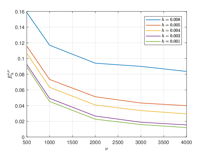
ν∈{500,1000,2000,3000,4000},h∈{0.008,0.005,0.004,0.002,0.001},\nu\in\{500,1000,2000,3000,4000\},\quad h\in\{0.008,0.005,0.004,0.002,0.001\},

we generate i.i.d. samples Ξν,k={ξ1k,…,ξνk},k=1,…,10000\Xi^{\nu,k}=\{\xi^{k}_{1},\ldots,\xi^{k}_{\nu}\},k=1,\ldots,10000. We solve the discrete problem to find a solution (xh,kϵ,ν,uh,kϵ,ν)(x^{\epsilon,\nu}_{h,k},u^{\epsilon,\nu}_{h,k}) using each of the samples Ξν,k\Xi^{\nu,k}, k=1,…,10000k=1,\ldots,10000. Then we compute the optimal value of the discrete problem for each kk

Φhν,k​(xh,kϵ,ν,uh,kϵ,ν)=1ν​∑i=1νF⁡(xh,kϵ,ν​(T),ξik)−12​(‖xh,kϵ,ν‖L22+‖uh,kϵ,ν‖L22).\Phi^{\nu,k}_{h}(x^{\epsilon,\nu}_{h,k},u^{\epsilon,\nu}_{h,k})=\frac{1}{\nu}\sum^{\nu}_{i=1}F(x^{\epsilon,\nu}_{h,k}(T),\xi^{k}_{i})-\frac{1}{2}(\|x^{\epsilon,\nu}_{h,k}\|^{2}_{L^{2}}+\|u^{\epsilon,\nu}_{h,k}\|^{2}_{L^{2}}).

The errors between Φ⁡(x∗,u∗)=25.17501124\Phi(x^{*},u^{*})=25.17501124 and the optimal value Φhν​(xhϵ,ν,uhϵ,ν)\Phi^{\nu}_{h}(x^{\epsilon,\nu}_{h},u^{\epsilon,\nu}_{h}) are estimated by

Ehϵ,ν=110000​∑k=110000(Φ⁡(x∗,u∗)−Φhν,k​(xh,kϵ,ν,uh,kϵ,ν))2.E_{h}^{\epsilon,\nu}=\frac{1}{10000}\sum^{10000}_{k=1}(\Phi(x^{*},u^{*})-\Phi^{\nu,k}_{h}(x^{\epsilon,\nu}_{h,k},u^{\epsilon,\nu}_{h,k}))^{2}.

The numerical results are shown in FIG. 1, which verify the convergence results in Sections 3-4.

Refer to caption
Refer to caption
Figure 1: Numerical errors between optimal values of (18) and its discrete problems

6 Conclusions

In this paper, we study the optimal control problem with terminal stochastic linear complementarity constraints (1), and its relaxation-SAA problem (9) and the relaxation-SAA-time stepping approximation problem (14). We prove the existence of feasible solutions and optimal solutions to problem (1) in Theorem 3 under the assumption E⁡[M⁡(ξ)]E[M(\xi)] is a Z-matrix or an adequate matrix. Under the same assumptions of Theorem 3, we prove the existence of feasible solutions and optimal solutions to (9) and (14). We also show the convergent properties of these two discrete problems (9) and (14) as the relaxation parameter ϵ↓0\epsilon\downarrow 0, the sample size ν→∞\nu\rightarrow\infty and mesh size h↓0h\downarrow 0. Moreover, we provide asymptotics of the SAA optimal value and the error bound of the time-stepping method. Problem (1) extends optimal control problem with terminal deterministic linear complementarity constraints in [2] to stochastic problems. In [2], Benita and Mehlita derived some stationary points and constraint qualifications under the assumption that the constrained LCP (2)-(3) is solvable. Theorem 3 gives sufficient conditions for the extension of solutions of (2)-(3).

References

  • [1] H. Attouch and R. J.-B. Wets, A convergence theory for saddle functions, Trans. Amer. Math. Soc., 280 (1983), pp. 1–41.
  • [2] F. Benita and P. Mehlitz, Optimal control problems with terminal complemenatrity constraints, SIAM J. Optim., 28 (2018), pp. 3079–3104.
  • [3] R. F. Brammer, Controllability in linear autonomous systems with positive controllers, SIAM J. Control Optim., 10 (1972), pp. 339–353.
  • [4] B. Brogliato, Some perspectives on the analysis and control of complementarity systems, IEEE T. Automat. Contr., 48 (2003), pp. 918–935.
  • [5] M. Brokate and P. Krejčí, Optimal control of ODE systems involving a rate independent variational inequality, Discrete Contin. Dyn. Syst. Ser. B, 18 (2013), pp. 331–348.
  • [6] X. Chen, First order conditions for nonsmooth discretized constrained optimal control problems, SIAM J. Control Optim., 42 (2004), pp. 2004–2015.
  • [7] X. Chen, R. J.-B. Wets, and Y. Zhang, Stochastic variational inequalities: residual minimization smoothing sample average approximations, SIAM J. Optim., 22 (2012), pp. 649–673.
  • [8] X. Chen and S. Xiang, Newton iterations in implicit time-stepping scheme for differential linear complementarity systems, Math. Program., 138 (2013), pp. 579–606.
  • [9] X. Chen and S. Xiang, Sparse solutions of linear complementarity problems, Math. Program., 159 (2016), pp. 539–556.
  • [10] C. Clason, Y. Deng, P. Mehlitz, and U. Prüfert, Optimal control problems with control complementarity constraints: existence results, optimality conditions, and a penalty method, Optim. Methods Softw., 35 (2020), pp. 142–170.
  • [11] R. W. Cottle, J.-S. Pang, and R. E. Stone, The Linear Complementarity Problem, Academic Press, Boston, 1992.
  • [12] A. L. Dontchev, Discrete approximations in optimal control, in Nonsmooth Analysis and Geometric Methods in Deterministic Optimal Control, B. S. Mordukhovich and H. J. Sussmann, eds., New York, NY, 1996, Springer New York, pp. 59–80.
  • [13] A. L. Dontchev and W. W. Hager, Euler approximation of the feasible set, Numer. Funct. Anal. Optim., 15 (1994), pp. 245–261.
  • [14] L. Guo and J. J. Ye, Necessary optimality conditions for optimal control problems with equilibrium constraints, SIAM J. Control Optim., 54 (2016), pp. 2710–2733.
  • [15] C. Heij, A. C. M. Ran, and F. van Schagen, Introduction to Mathematical Systems Theory: Discrete Time Linear Systems, Control and Identification (Second Edition), Birkhäuser Cham, Gewerbestrasse, 2021.
  • [16] P. Lambrianides, Q. Gong, and D. Venturi, A new scalable algorithm for computational optimal control under uncertainty, J. Comput. Phys., 420 (2020), p. 109710.
  • [17] P. Mehlitz and G. Wachsmuth, Bilevel Optimal Control: Existence Results and Stationarity Conditions, Springer International Publishing, Cham, 2020, pp. 451–484.
  • [18] B. S. Mordukhovich and T. Pennanen, Epi-convergent discretization of the generalized bolza problem in dynamic optimization, Optim. Lett., 1 (2007), pp. 379–390.
  • [19] C. Phelps, Q. Gong, J. O. Royset, C. Walton, and I. Kaminer, Consistent approximation of a nonlinear optimal control problem with uncertain parameters, Automatica, 50 (2014), pp. 2987–2997.
  • [20] C. Phelps, J. O. Royset, and Q. Gong, Optimal control of uncertain systems using sample average approximations, SIAM J. Control Optim., 54 (2016), pp. 1–29.
  • [21] O. L. Pironneau and E. Polak, Consistent approximations and approximate functions and gradients in optimal control, SIAM J. Control Optim., 41 (2002), pp. 487–510.
  • [22] A. U. Raghunathan, M. S. Diaz, and L. T. Biegler, An MPEC formulation for dynamic optimization of distillation operations, Comput. Chem. Eng., 28 (2004), pp. 2037–2052.
  • [23] A. Shapiro, D. Dentcheva, and A. Ruszczynski, Lectures on Stochastic Programming: Modeling and Theory, SIAM, Philadelphia, 2009.
  • [24] A. Vieira, B. Brogliato, and C. Prieur, Quadratic optimal control of linear complementarity systems: first order necessary conditions and numerical analysis, IEEE T. Automat. Contr., 65 (2020), pp. 1168–1175.
  • [25] H. Yoshida and T. Tanaka, Positive controllability test for continuous-time linear systems, IEEE T. Automat. Contr., 52 (2007), pp. 1685–1689.