Kinodynamic Control Systems and Discontinuities in Clearance

Niles Armstrong Email address, A1 : armstrongn@msoe.edu , Jory Denny Email address, A2 : joryldenny@gmail.com and Jeremy LeCrone Email address, A3 : jlecrone@richmond.edu

Abstract.

We investigate the structure of discontinuities in clearance (or minimum time) functions for nonlinear control systems with general, closed obstacles (or targets). We establish general results regarding interactions between admissible trajectories and clearance discontinuities: e.g. instantaneous increases in clearance when passing through a discontinuity, and propagation of discontinuity along optimal trajectories. Then, investigating sufficient conditions for discontinuities, we explore a common directionality condition for velocities at a point, characterized by strict positivity of the minimal Hamiltonian. Elementary consequences of this common directionality assumption are explored before demonstrating how, in concert with corresponding obstacle configurations, it gives rise to clearance discontinuities both on the surface of the obstacle and propagating out into free space. Minimal assumptions are made on the topological structure of obstacle sets.

Key words and phrases:

Control theory, Minimal time function, Discontinuous value function

2010 Mathematics Subject Classification

93C10, 49N60, 93B03

1. Introduction

This paper studies nonlinear optimal control problems in constrained environments and fine properties of associated clearance functions (or minimal time functions in time–optimal settings). We focus on settings where discontinuities in clearance arise and investigate the fine analytic structure of these sets of discontinuities when systems admit a strict directionality of admissible velocities.

As motivation for this investigation, we note that optimal control is relevant to questions in robotics, mechanical engineering, and aerospace engineering. Specifically, algorithms that plan the motion of dynamical systems from a start state to a goal region (motion planning algorithms) may exploit many of the properties of discontinuities we explore herein. As an example of one such class of algorithms, Rapidly–exploring Random Trees (RRTs) build approximate representations of a robot’s state space that encode feasible pathways for a robot to move through regions of a constrained state space [16]. These methods seek not only to find the existence of feasible paths, but paths with cost optimality [15] (e.g., minimal time or shortest distance) and safety guarantees [12] to ensure reliable clearance from obstacles.

Although clearance is traditionally interpreted as a robot’s geometric distance from obstacles (with respect to canonical metrics in state space) we embrace a system–dependent perspective on clearance. As observed in applications (c.f., [22]), the dynamic limitations of a robot’s motion should also receive proper consideration in questions of optimality and safety of admissible trajectories. Such considerations lead one naturally to a formulation of clearance that ignores obstacles outside the accessible region of a robot (c.f., Definition 2.2), which corresponds with the minimal time function (in time–optimal settings) studied extensively in the mathematical control theory community [1, 4, 5, 6, 11, 14, 18, 20, 23, 24].

The regularity of clearance / minimal–time functions is an active area of research, with a large selection of literature dedicated to sufficient conditions ensuring regularity conditions near obstacles. As a small sampling of this literature, we point the interested reader to a selection of references discussing differentiability [6], continuity and semicontinuity [24], and semiconcavity [5] of minimal–time functions. A ubiquitous assumption in these studies is the controllability of the system in a neighborhood of the obstacle set, classically exemplified by the Petrov condition (c.f., [9]). Essentially, this condition enforces the existence of admissible velocities at all obstacle boundary points so that trajectories reasonably penetrate the obstacle. Our investigation diverges from those efforts, which we mention primarily to highlight the fact that we will be working in settings devoid of such Petrov–type controllability conditions.

It is well–known that discontinuities arise in optimal control settings (c.f., [2, 3, 7, 13]), though there has been little attention paid to the precise analytic structure of these discontinuities in clearance. This paper presents a framework for this analysis along with a number of important initial results to be built upon in future investigations. Further, as motivated above, we note that this work can potentially inform future developments in robot motion planning.

We proceed with a brief outline of the paper. In Section 2, we introduce the setting, assumptions, and definitions for the investigation. We observe that the optimal cost–distance produces a quasi-metric on state space (a form of asymmetric distance between states) associated to which we identify quasi-metric cost–balls centered at a given state. The geometric properties of these evolving cost–balls plays an important role in the analysis of discontinuities in clearance.

In Section 3, we isolate an assumption of directionality among admissible velocities – quantified by strict positivity of the minimal Hamiltonian Equation 2.5 – in the direction of some vector $\xi.$ We state and prove a number of elementary consequences of this strict directionality, including a type of small–time–local–non–returnability (Lemma 3.4) and existence of persistent boundary points (Theorem 3.5) on corresponding reachable sets. Embodied in this persistent boundaries result is an investigation of a local envelope of propagating reachable sets, a concept that is central to the analysis of discontinuities of clearance in free space.

In Section 4, we establish intrinsic properties of clearance; i.e. properties of clearance as one traverses admissible trajectories. Notably, in Theorem 4.4, we confirm that clearance cannot discontinuously decrease along admissible trajectories.

Finally, in Section 5 we study properties of discontinuities in clearance. First, we characterize all discontinuities in free space (Theorem 5.3) as envelope points on the boundaries of multiple members of a family of propagating reachable waves (Definition 5.1). These envelope points are further shown to form a continuous structure in space (Theorem 5.5), propagated along optimal trajectories back to the obstacle set. Next, we turn our attention to clearance discontinuities present on the boundary of the obstacle set itself. After a brief exploration of general properties, we focus specifically on a type of envelope generator discontinuity (Definition 5.8); from which free space discontinuities propagate with arbitrarily small clearance.

Our main result is Theorem 5.12, providing a set of sufficient conditions ensuring an obstacle boundary point is in fact an envelope generator. Thus ensuring the existence of free space discontinuities nearby. This result is preceded by motivating examples and followed by applications of the result.

2. Definitions and Assumptions

2.1. General Setting

Let ${\mathcal{X}_{space}}\subseteq\mathbb{R}^{n}$ be state space, with inner product denoted $\langle\cdot,\cdot\rangle,$ and let $\mathcal{U}_{space}\subseteq\mathbb{R}^{m}$ be control space. We fix a state function $f:{\mathcal{X}_{space}}\times\mathcal{U}_{space}\to{\mathcal{X}_{space}},$ with regularity conditions to be addressed below. Given two states $x,y\in{\mathcal{X}_{space}},$ we denote by $\Pi_{u}(x,y)$ the collection of absolutely continuous trajectories $\pi:[0,T]\to{\mathcal{X}_{space}}$ solving the parameterized control problem

(2.1)

\begin{cases}\dot{\pi}(t)=f(x(t),u(t))&\text{a.e. $t\in[0,T]$}\\ u(t)\in\mathcal{U}_{space}&\text{a.e. $t\in[0,T]$}\\ \pi(0)=x,\\ \pi(T)=y,\end{cases}

for some $T=T_{\pi}\geq 0.$ We say that $\pi\in\Pi_{u}(x,y)$ is an unconstrained trajectory moving $x$ to $y$ in $T_{\pi}$ units of time. Further, we fix a continuous running cost function $\psi:{\mathcal{X}_{space}}^{2}\to(0,\infty),$ with which one computes the cost to traverse $\pi\in\Pi_{u}(\cdot,\cdot)$ as

(2.2)

c_{\pi}:=\int_{0}^{T_{\pi}}\psi(\pi(t),\dot{\pi}(t))dt.

To address the regularity conditions for the state function, we shift our discussion to the equivalent nonparameterized control system. Namely, we define the admissible velocity multifunction (i.e. set–valued function)

(2.3)

F:{\mathcal{X}_{space}}\rightrightarrows{\mathcal{X}_{space}}\qquad\text{with}\qquad F(x):=\{f(x,u):u\in\mathcal{U}_{space}\}.

Under mild assumptions, it is well known that $\Pi_{u}(x,y)$ coincides with the absolutely continuous solutions to the differential inclusion

(2.4)

\begin{cases}\dot{\pi}(t)\in F(\pi(t))&\text{for a.e. $t\in[0,T]$}\\ \pi(0)=x,\\ \pi(T)=y.\end{cases}

We direct the interested reader to standard introductory texts in mathematical control theory [3, 10] for further details on this and other standard results.

Finally, we adopt the following standard assumptions on velocity sets, which (albeit indirectly) address assumptions one can make for state functions $f.$

Assumption 2.1 (Standing Hypotheses for Velocity Sets).

(SH1)

(Nonempty, closed, bounded, convex velocity sets) For all $x\in{\mathcal{X}_{space}},$ the set $F(x)\subset{\mathcal{X}_{space}}$ is nonempty and convex, with graph $grF:=\{(x,v):v\in F(x)\}$ closed in ${\mathcal{X}_{space}}^{2}$ , and for each compact set $K\subset{\mathcal{X}_{space}},$ there exists a constant $M>0$ so that $\sup\{\|v\|:x\in K,v\in F(x)\}\leq M.$
(SH2)

(Linear growth condition) There exist $\gamma,c>0$ so that for all $x\in{\mathcal{X}_{space}}$ it holds that $\|v\|\leq\gamma\|x\|+c$ whenever $v\in F(x).$
(SH3)

(Local Lipschitz regularity) For each compact set $K\subset{\mathcal{X}_{space}},$ there exists $k>0$ such that

$F(x)\subseteq F(y)+k\|x-y\|\overline{B_{1}(0)}\qquad\text{for all $x,y\in K,$}$

where $\overline{B_{1}(0)}$ denotes the closed unit ball centered at $0\in{\mathcal{X}_{space}}.$

We also define the minimal (or lower) Hamiltonian at a point $x\in{\mathcal{X}_{space}},$ in the direction of some vector $\xi\in{\mathcal{X}_{space}},$ as

(2.5)

h_{F}(x,\xi):=\inf_{v\in F(x)}\langle v,\xi\rangle.

Informally, we note that $h_{F}(x,\xi)>0$ means all admissible velocities at $x$ have a nontrivial positive component in the $\xi$ direction.

We introduce kinodynamic constraints on our control system by way of the following identification of obstacles in ${\mathcal{X}_{space}}.$ Let ${\mathcal{X}_{obst}}\subset{\mathcal{X}_{space}}$ be any closed obstacle set and denote by ${\mathcal{X}_{free}}:={\mathcal{X}_{space}}\setminus{\mathcal{X}_{obst}}$ the open free space within whose closure trajectories are constrained. In particular, with ${\mathcal{X}_{obst}}$ and ${\mathcal{X}_{free}}$ fixed, we define the collection of admissible trajectories moving $x\in{\mathcal{X}_{space}}$ to $y\in{\mathcal{X}_{space}}$ as

\Pi(x,y):=\{\pi\in\Pi_{u}(x,y):\pi(t)\in\overline{{\mathcal{X}_{free}}}\quad\text{for all $t\in[0,T_{\pi}]$}\}.

Note that $\Pi(x,y)=\emptyset$ whenever $x$ or $y$ are in the interior of the obstacle set, ${\mathcal{X}_{obst}}^{\circ}.$

The following definitions lay the foundations for analysis in ${\mathcal{X}_{space}},$ using the intrinsic system–dependent cost–distance between states. We mention that our assumption of positive running cost (i.e. $\psi>0$ ) means that one could reformulate our problem to a simple minimal–time problem (i.e. with $\psi\equiv 1$ and $c_{\pi}\equiv T_{\pi}$ ) throughout (c.f. [3, Remark 6.7]). We take advantage of this equivalence to support application of known results from the literature, but maintain a framework with general running–cost functions for accessibility of our results in applications.

Definition 2.2.

Given $x,y\in{\mathcal{X}_{space}}$ and $\rho>0,$ we define the following:

The control–system–dependent distance (or cost–distance) from $x$ to $y$

d_{c}(x,y):=\begin{cases}\inf\{c_{\pi}:\pi\in\Pi(x,y)\}&\text{if $\Pi(x,y)\neq\emptyset$}\\ \infty&\text{if $\Pi(x,y)=\emptyset.$}\end{cases}

b)

The forward reachable set of radius $\rho$

$\mathcal{F}_{\rho}(x):=\{y\in{\mathcal{X}_{space}}:d_{c}(x,y)<\rho\}.$
c)

The reverse reachable set of radius $\rho$

$\mathcal{R}_{\rho}(x):=\{y\in{\mathcal{X}_{space}}:x\in\mathcal{F}_{\rho}(y)\}.$
d)

The clearance from ${\mathcal{X}_{obst}}$

$\textsc{clr}(x):=\inf_{y\in{\mathcal{X}_{obst}}}d_{c}(x,y).$
e)

The set of witness points

$\textsc{wit}(x):=\{y\in{\partial{\mathcal{X}_{obst}}}:d_{c}(x,y)=\textsc{clr}(x)\}.$

In general, the cost–distance function forms a quasi–metric on ${\mathcal{X}_{space}}.$ That is, $d_{c}(x,y)\geq 0$ with $d_{c}(x,y)=0$ if and only if $x=y,$ and $d_{c}(x,y)\leq d_{c}(x,z)+d_{c}(z,y)$ for all $x,y,z\in{\mathcal{X}_{space}},$ but $d_{c}(x,y)\neq d_{c}(y,x)$ in general. We introduce the quasi–metric cost balls,

\mathcal{B}_{\rho}(x):=\mathcal{F}_{\rho}(x)\cup\mathcal{R}_{\rho}(x)\qquad\text{for $x\in{\mathcal{X}_{space}}.$}

We conclude this section by exploring the connections between the standard metric induced by norm $\|\cdot\|_{{\mathcal{X}_{space}}}$ and the quasi–metric here introduced. To complement the quasi–metric ball around $x,$ we denote the standard metric ball of radius $r>0$ centered at $x$ as

B_{r}(x):=\{y\in{\mathcal{X}_{space}}:\|x-y\|_{{\mathcal{X}_{space}}}<r\}.

(Throughout, we adopt the convention that roman letters $r,s,t$ denote radii for metric balls, while Greek letters $\rho,\mu,\eta$ denote radii for cost balls.)

Now we list a number of elementary properties that are needed for future analysis. The proofs for these facts follow from standard arguments, with references (or proof ideas) provided as appropriate.

Proposition 2.3 (Properties of cost and clearance).

Suppose $x,y\in{\mathcal{X}_{space}}$

a)

[24, Proposition 2.2(a)] The sets $\mathcal{R}_{\rho}(x)$ and $\mathcal{F}_{\rho}(x)$ evolve continuously in $\rho,$ with respect to the Hausdorff distance.
b)

[24, Proposition 2.4] If sequences $(x_{n}),(y_{n})\subset{\mathcal{X}_{space}}$ converge to $x$ and $y,$ respectively, and $\pi_{n}\in\Pi(x_{n},y_{n})$ exist with $c_{\pi_{n}}\to c,$ then there exists $\pi\in\Pi(x,y)$ with $c_{\pi}=c.$
c)

[24, Proposition 2.6] If $\Pi(x,y)\neq\emptyset,$ then there exists an optimal trajectory $\pi\in\Pi(x,y)$ with $c_{\pi}=d_{c}(x,y).$ Moreover, if $\textsc{clr}(x)<\infty,$ then $\textsc{wit}(x)\neq\emptyset$ and, for all $y\in\textsc{wit}(x),$ there exists an optimal $\pi\in\Pi(x,y)$ with $c_{\pi}=\textsc{clr}(x).$
d)

[9, Theorem 3.11] The sets $\mathcal{F}_{\rho}(x)$ are locally Lipschitz continuous in $x,$ with respect to the Hausdorff distance. More precisely, we have that the forward attainable sets

$\mathcal{A}_{\rho}(x):=\{y\in{\mathcal{X}_{space}}:c_{\pi}=\rho\text{ for some }\pi\in\Pi(x,y)\}$

have local Lipschitz continuous dependence on $x.$
e)

Given $0<\rho<\mu,$ it holds that $\overline{\mathcal{B}_{\rho}(x)}\subseteq\mathcal{B}_{\mu}(x).$
(This is a straightforward consequence of property (b) above)

3. Consequences of Positive Hamiltonian

As motivated in the introduction, a strict directionality of admissible velocities is the primary driving force in our analysis of clearance discontinuities. We establish in this section some of the preliminary consequences of this assumption.

Throughout this section, we assume that $x,\xi\in{\mathcal{X}_{space}}$ are given with $\xi\neq 0$ and satisfying the property

(3.1)

h_{F}(x,\xi):=\inf_{v\in F(x)}\langle v,\xi\rangle>0.

Further, given any $r^{\star}>0$ we define a point that is a geometric distance of $r^{\star}$ away from $x$ in the direction of $\xi,$ namely

x^{\star}:=x+\frac{r^{\star}}{\|\xi\|}\xi.

Proposition 3.1.

Given $h_{F}(x,\xi)>0$ and $r^{\star}>0,$ then there exists $R\in(0,r^{\star})$ so that $h_{F}(y,x^{\star}-y)>\frac{1}{2}h_{F}(x,x^{\star}-x)$ for all $y\in\overline{B_{R}(x).}$

Proof.

This is a straightforward consequence of standing hypotheses (SH1) and (SH3). We include details of the proof for the reader’s convenience.

By compactness of $\overline{B_{2r^{\star}}(x)},$ fix values $M>0$ and $K>0$ so that

(3.2)

y\in\overline{B_{2r^{\star}}(x)}\quad\text{and}\quad v\in F(y)\quad\Longrightarrow\quad\|v\|\leq M,

and

(3.3)

y,z\in\overline{B_{2r^{\star}}(x)}\quad\Longrightarrow\quad F(y)\subset F(z)+K\|y-z\|\overline{B_{1}(0)}.

Select any $y\in\overline{B_{2r^{\star}}(x)}$ and $w\in F(y).$ It follows from Equation 3.3 that

w=v_{w}+K\|x-y\|\phi_{w},\qquad\text{for some}\qquad v_{w}\in F(x),\ \phi_{w}\in\overline{B_{1}(0)}.

Employing Cauchy–Schwarz inequality, we compute

	$\displaystyle\langle w,x^{\star}-$	$\displaystyle y\rangle=\langle v_{w},x^{\star}-x\rangle+\langle v_{w},x-y\rangle+K\\|x-y\\|\langle\phi_{w},x^{\star}-y\rangle$
		$\displaystyle\geq h_{F}(x,x^{\star}-x)-\|\langle v_{w},x-y\rangle\|-K\\|x-y\\|\|\langle\phi_{w},x^{\star}-y\rangle\|$
		$\displaystyle\geq h_{F}(x,x^{\star}-x)-\\|v\\|\\|x-y\\|-K\\|x-y\\|\\|\phi_{w}\\|\\|x^{\star}-y\\|$
		$\displaystyle\geq h_{F}(x,x^{\star}-x)-\\|x-y\\|\big(M+3r^{\star}K\big).$

The claim thus follows with any selection of $0<R<h_{F}(x,x^{\star}-x)/2\big(M+3r^{\star}K\big).$ To see that $R<r^{\star},$ note $h_{F}(x,x^{\star}-x)\to 0$ as $x\to x^{\star},$ and so $x^{\star}\notin\overline{B_{R}(x)}.$ ∎

Proposition 3.2.

Given $h_{F}(x,\xi)>0$ and $r^{\star}>0,$ there exists $t^{\star}>0$ so that

\frac{d}{dt}\|x^{\star}-\pi(t)\|\leq-\frac{h_{F}(x,x^{\star}-x)}{r^{\star}}

for all maximally--defined trajectories¹¹ 1 By maximally–defined in the unconstrained setting, we simply consider trajectories that have been extended (as necessary) to a maximal time interval; i.e. so that $T_{\pi}=\infty.$ $\pi\in\Pi_{u}(x,\cdot)$ and a.e. $t\in[0,t^{\star}].$

Proof.

Proceeding from the proof of Proposition 3.1, we select any value

0<t^{\star}<\frac{R}{M}.

Now, consider a maximally–defined trajectory $\pi\in\Pi_{u}(x,\cdot).$ Given $t\in[0,t^{\star}],$ first observe that $\pi(t)\in B_{R}(x)\subset B_{2r^{\star}}(x)$ by Equation 3.2, since

\|\pi(t)-x\|\leq\int_{0}^{t}\|\dot{\pi}(s)\|ds\leq Mt<R<r^{\star}.

Select an arbitrary vector $w\in F(\pi(t)).$ It follows from Equation 3.3 that

w=v_{w}+K\|x-\pi(t)\|\phi_{w},\qquad\text{for some}\qquad v_{w}\in F(x),\ \phi_{w}\in\overline{B_{1}(0)}.

Thus, by Proposition 3.1, we compute

(3.4)

\begin{split}\frac{d}{dt}\|x^{\star}-\pi(t)\|^{2}&=\frac{d}{dt}\big\langle x^{\star}-\pi(t),x^{\star}-\pi(t)\big\rangle\\ &\leq-2h_{F}(\pi(t),x^{\star}-\pi(t))\leq-h_{F}(x,x^{\star}-x),\end{split}

noting the computation is valid for a.e. $t\in[0,t^{\star}],$ by absolute continuity of $\pi(\cdot).$ ∎

The following two lemmas are consequences of the previous propositions. The first result provides a quantitative statement for uniform directional propagation (Figure 1a is a visualization of this phenomenon). The second lemma quantifies a type of non–small–time–local–controllability present whenever Equation 3.1 holds.

Lemma 3.3.

Given $h_{F}(x,\xi)>0$ and $r^{\star}>0,$ set $t^{\star}>0$ as in Proposition 3.2. Then, for every $t\in(0,t^{\star}],$ there exists $\eta^{\star}=\eta^{\star}(t)\in(0,1)$ so that

\pi(t)\in B_{\eta^{\star}r^{\star}}(x^{\star})

for all maximally–defined trajectories $\pi\in\Pi_{u}(x,\cdot).$

Proof.

Proceeding from Proposition 3.2, we compute

\|x^{\star}-\pi(t)\|^{2}=(r^{\star})^{2}+\int_{0}^{t}\frac{d}{ds}\|x^{\star}-\pi(s)\|^{2}ds\leq(r^{\star})^{2}-th_{F}(x,x^{\star}-x).

It follows that $\|x^{\star}-\pi(t)\|<\eta^{\star}r^{\star}=\eta^{\star}\|x^{\star}-x\|$ for any choice of parameter

1>\eta^{\star}>\left(1-\frac{th_{F}(x,x^{\star}-x)}{(r^{\star})^{2}}\right)^{1/2}.\qed

Lemma 3.4.

Suppose $x\in{\mathcal{X}_{free}}$ and $\xi\in{\mathcal{X}_{space}}$ with $h_{F}(x,\xi)>0.$ Then there exists $\rho^{\star}=\rho^{\star}(x)>0$ so that for all $\rho\in(0,\rho^{\star}),$ there exists $r(\rho)=r(\rho,x)>0$ with

\mathcal{B}_{\rho^{\star}}(x)\setminus\mathcal{B}_{\rho}(x)\subset\big(B_{r(\rho)}(x)\big)^{c}.

Equivalently, if $y\in{\mathcal{X}_{space}}$ with $\rho\leq\min\{d_{c}(x,y),d_{c}(y,x)\}<\rho^{\star},$ then $\|x-y\|\geq r(\rho)=r(\rho,x).$

Proof.

By ${\mathcal{X}_{free}}$ open, we select $r^{\star}>0$ so that $B_{r^{\star}}(x)\subset{\mathcal{X}_{free}}.$ Now, we fix $R>0$ as in Proposition 3.1, $t^{\star}>0$ as in Proposition 3.2, and select $\rho^{\star}=\rho^{\star}(x)>0$ sufficiently small that $\mathcal{B}_{\rho^{\star}}(x)\subset B_{R}(x).$ By compactness of $\overline{B_{R}(x)},$ standing hypothesis (SH1), and continuity of $\psi,$ we define

(3.5)

\psi^{\star}:=\max\{\psi(y,v):y\in\overline{B_{R}(x)},v\in F(y)\}.

Now, let $\rho\in(0,\rho^{\star}),$ apply Lemma 3.3 to set

\eta^{\star}=\eta^{\star}\big(\min\left\{t^{\star},\rho/\psi^{\star}\right\}\big)

and define $r(\rho)=r^{\star}-\eta^{\star}r^{\star}.$

Consider any trajectory $\pi\in\Pi_{u}(x,\cdot)\cup\Pi_{u}(\cdot,x)$ with $\rho\leq c_{\pi}<\rho^{\star}.$ We note that $\mathcal{B}_{\rho^{\star}}(x)\subset{\mathcal{X}_{free}},$ so all such unconstrained trajectories are likewise admissible (constrained) trajectories. It follows from Equation 2.2 that $T_{\pi}\geq\frac{\rho}{\psi^{\star}},$ and we conclude the proof with the observation that

\pi(T_{\pi})\in B_{\eta^{\star}r^{\star}}(x^{\star})\subset\big(B_{r(\rho)}(x)\big)^{c}.\qed

In the next result, we demonstrate how Equation 3.1 gives rise to the existence of persistent boundary points on reachable sets (Figure 1b). The presence of such persistent boundary points, within families of propagating sets, plays a key role in the analysis of clearance discontinuities in Section 5 below.

Theorem 3.5.

Suppose $x\in{\mathcal{X}_{free}}$ and $\xi\in{\mathcal{X}_{space}}$ with $h_{F}(x,\xi)>0.$ For all $r>0$ there exists $\rho>0$ so that

\big(\partial\mathcal{R}_{\rho}(x)\cap\partial\mathcal{R}_{\mu}(x)\cap B_{r}(x)\big)\setminus\{x\}\neq\emptyset\qquad\text{for all $0<\mu<\rho,$}

and

\big(\partial\mathcal{F}_{\rho}(x)\cap\partial\mathcal{F}_{\mu}(x)\cap B_{r}(x)\big)\setminus\{x\}\neq\emptyset\qquad\text{for all $0<\mu<\rho.$}

Proof.

Given $r>0,$ choose $0<r^{\star}\leq r$ so that $B_{r^{\star}}(x)\subset{\mathcal{X}_{free}}$ and set $x^{\star}:=x+\frac{r^{\star}}{\|\xi\|}\xi.$ Applying Propositions 3.1 and 3.4, we fix $R>0$ and $\rho^{\star}(x)>0$ . Choose any $\rho\in(0,\rho^{\star}(x))$ sufficiently small that $\mathcal{B}_{\rho}(x)\subseteq B_{R}(x).$

We claim that

(3.6)

\mathcal{R}_{\rho}(x)\setminus\{x\}\subset\big(B_{r^{\star}}(x^{\star})\big)^{c}.

Indeed, given $y\in\mathcal{R}_{\rho}(x)$ and $\pi\in\Pi(y,x)$ with $c_{\pi}<\rho,$ consider any $\tau\in[0,T_{\pi}].$ Since $\pi(\tau)\in B_{R}(x),$ we know that $h_{F}(\pi(\tau),x^{\star}-\pi(\tau))>0.$ It follows from Proposition 3.2 that $\|x^{\star}-\pi(\tau+t)\|$ is strictly decreasing on some interval $t\in[0,t^{\star}(\tau)].$ By compactness of the interval $[0,T_{\pi}],$ we conclude $\|x^{\star}-\pi(t)\|$ is strictly decreasing from $y$ to $x.$ Therefore, we have $\|x^{\star}-y\|>\|x^{\star}-x\|=r^{\star}.$

Let $0<\mu<\rho.$ Fix $r(\mu)=r(\mu,x)$ as in Lemma 3.4 and then select

\tilde{r}:=\min\{r,r(\mu)\}.

Consider the deleted neighborhood $\mathcal{N}:=B_{\tilde{r}}(x)\setminus\{x\}.$ Note that $\mathcal{N}\cap\mathcal{R}_{\rho}(x)\neq\emptyset,$ while $\mathcal{N}\cap\big(\mathcal{R}_{\rho}(x)\big)^{c}\neq\emptyset$ follows from Equation 3.6. Since $\mathcal{N}$ is a connected set, we conclude

\mathcal{N}\cap\partial\mathcal{R}_{\rho}(x)\neq\emptyset.

Let $z\in\mathcal{N}\cap\partial\mathcal{R}_{\rho}(x).$ Proposition 2.3(e) and $\rho<\rho^{\star}(x)$ imply that $d_{c}(z,x)<\rho^{\star}(x).$ Moreover, since $\|z-x\|<\tilde{r}\leq r(\mu)$ , we conclude $d_{c}(z,x)<\mu,$ from Lemma 3.4. Therefore, we have that $z\in\mathcal{R}_{\mu}(x)\cap\partial\mathcal{R}_{\rho}(x)$ which implies

z\in\partial\mathcal{R}_{\mu}(x)\cap\partial\mathcal{R}_{\rho}(x)\cap\mathcal{N}\subseteq\big(\partial\mathcal{R}_{\rho}(x)\cap\partial\mathcal{R}_{\mu}(x)\cap B_{r}(x)\big)\setminus\{x\}.

A symmetric argument proves the result for forward reachable sets. Therein, Eq. 3.6 is replaced by $\mathcal{F}_{\rho}(x)\setminus\{x\}\subset B_{r^{\star}}(x^{\star}),$ which follows directly from Proposition 3.2. ∎

4. Intrinsic Properties of Clearance

Having established preliminary results regarding cost balls, we turn now to expand on the behavior of the clearance function $\textsc{clr}.$ In particular, we focus on properties of clr observable as one traverses along admissible trajectories (i.e. an intrinsic perspective to objects moving in the system).

Proposition 4.1.

For all $x,z\in{\mathcal{X}_{space}},$ we have $\textsc{clr}(x)\leq\textsc{clr}(z)+d_{c}(x,z).$

Proof.

This is a straightforward result from an extended trajectory. Namely, suppose we have $\pi\in\Pi(x,z),\ y\in\textsc{wit}(z),$ and $\pi^{\prime}\in\Pi(z,y)$ so that $c_{\pi}=d_{c}(x,z)$ and $c_{\pi^{\prime}}=\textsc{clr}(z).$ It follows that the trajectory

\hat{\pi}(t):=\begin{cases}\pi(t)&\text{for $t\in[0,T_{\pi}]$}\\ \pi^{\prime}(t-T_{\pi})&\text{for $t\in[T_{\pi},T_{\pi}+T_{\pi^{\prime}}]$}\end{cases}

is an element of $\Pi(x,y).$ Thus, we compute

\textsc{clr}(x)\leq c_{\hat{\pi}}=c_{\pi^{\prime}}+c_{\pi}=\textsc{clr}(z)+d_{c}(x,z).\qed

Remark 4.2.

Extending Proposition 4.1, we observe that

(4.1)

\textsc{clr}(x)-\textsc{clr}(z)\leq d_{c}(x,z)\qquad\text{whenever}\qquad\textsc{clr}(z)<\infty.

Intuition from geometric settings may lead one to expect the difference $\textsc{clr}(z)-\textsc{clr}(x)$ to also be bounded above by $d_{c}(x,z).$ We demonstrate the fallacy of this attempt with the following example.

Example 4.3 (Galaga System²² 2 Inspired by the classic 1981 arcade game of the same name and its subsequent incarnations.).

Working in ${\mathcal{X}_{space}}=\mathbb{R}^{2},$ we consider the system

(4.2)

\begin{cases}\dot{x}_{1}=u\\ \dot{x}_{2}=1\end{cases}\qquad\text{for}\qquad u\in\mathcal{U}_{space}:=[-1,1].

For simplicity, we set $\psi\equiv 1,$ so that $c_{\pi}=T_{\pi}$ for all trajectories. We constrain ${\mathcal{X}_{free}}$ to be a vertical passage opening into a wider passage at $x_{2}=0.$ Precisely, we set

	$\displaystyle{\mathcal{X}_{free}}$	$\displaystyle:=(-1,2)\times(-\infty,0]\ \bigcup\ (-5,2)\times(0,\infty)\qquad\text{and}$
	$\displaystyle{\mathcal{X}_{obst}}$	$\displaystyle:={\mathcal{X}_{space}}\setminus{\mathcal{X}_{free}}.$

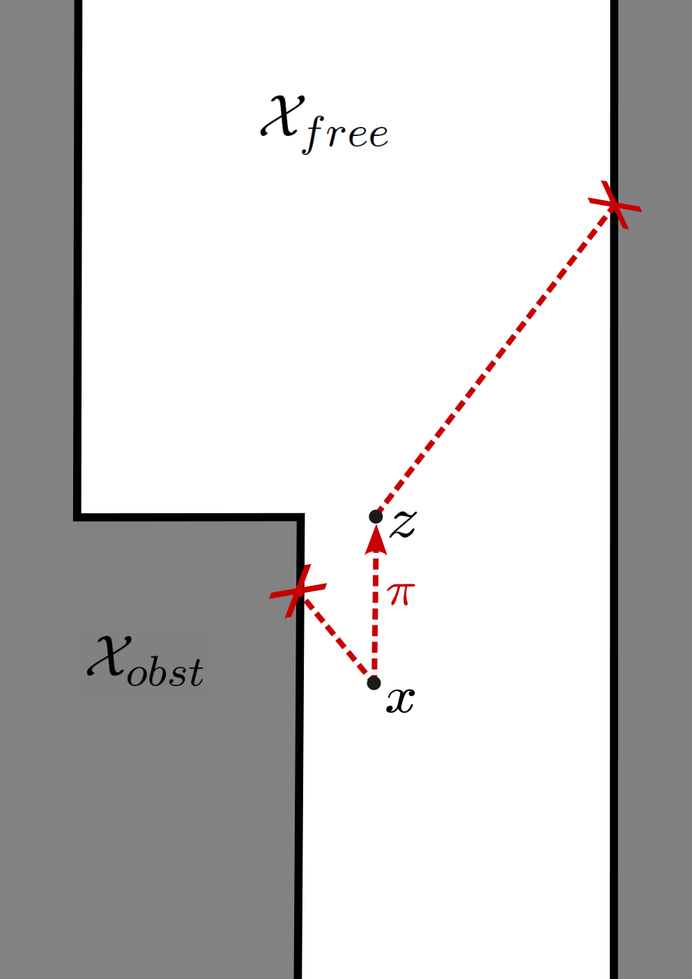
Consider $x=\left(-\frac{1}{2},-1\right)$ and $z=\left(-\frac{1}{2},0\right).$ Then, one computes (c.f. Figure 2a)

•

$d_{c}(x,z)=1,$ realized by $\pi(t)=\left(-\frac{1}{2},-1+t\right)$ with controls $u(t)\equiv 0,$
•

$\textsc{clr}(x)=1/2,$ with $\textsc{wit}(x)=\left\{\left(-1,-\frac{1}{2}\right)\right\},$ and
•

$\textsc{clr}(z)=5/2,$ with $\textsc{wit}(z)=\left\{\left(2,\frac{5}{2}\right)\right\}$ .

Thus confirming the discussion in Remark 4.2 above, observing here that we have

(4.3)

\textsc{clr}(z)-\textsc{clr}(x)>d_{c}(x,z).

We also note that a discontinuous jump in clr occurs in Figure 2a when the trajectory $\pi$ passes through the point $\left(-\frac{1}{2},-\frac{1}{2}\right).$ In fact, we confirm in Corollary 5.4 that this is the only type of discontinuity that may occur along admissible trajectories.

Further, modifying the structure of ${\mathcal{X}_{free}},$ we can produce Equation 4.3 without passing through a discontinuity in $\textsc{clr}(\pi(\cdot)).$ Set

{\mathcal{X}_{free}}=(-1,\infty)\times(-\infty,0]\ \bigcup\ \{(x_{1},x_{2}):x_{2}>-2x_{1}-2\text{ and }x_{2}>0\},

noting that ${\mathcal{X}_{free}}$ is no longer a long passageway, but rather an unbounded region with only one wall bounding motion in the negative $x_{1}$ direction.

Now, we consider $x=\left(-\frac{1}{2},-1\right)$ and $z=\left(-\frac{1}{2},2\right).$ Then, we have $d_{c}(x,z)=3,$ while $\textsc{clr}(z)=5$ and $\textsc{clr}(x)=\frac{1}{2},$ which satisfies Equation 4.3. We leave it as an exercise for the reader to confirm clr is continuous everywhere in this modified setting.

The following result establishes the (one–sided) limits of clr at points along admissible trajectories.

Theorem 4.4.

Given an admissible trajectory $\pi\in\Pi(\cdot,\cdot)$ and $\tau\in(0,T_{\pi})$ for which $\textsc{clr}(\pi(\tau))<\infty,$ it holds that

\lim_{t\to\tau^{-}}\ \textsc{clr}(\pi(t))\leq\textsc{clr}(\pi(\tau))\leq\lim_{t\to\tau^{+}}\ \textsc{clr}(\pi(t)).

Proof.

We will first establish the existence of the one–sided limits at $\tau.$

Regarding the limit $t\nearrow\tau,$ observe that $\textsc{clr}(\pi(t))<\infty$ for all $t\in[0,\tau]$ by Proposition 4.1 and assumption that $\textsc{clr}(\pi(\tau))<\infty.$ Let $\varepsilon>0,$ and fix $0<\delta$ with $\int_{\tau-\delta}^{\tau}\psi(\pi(t),\dot{\pi}(t))dt<\frac{\varepsilon}{2}.$ Next, we fix $t^{\star}\in(\tau-\delta,\tau)$ so that

\textsc{clr}(\pi(t^{\star}))>\sup_{t\in(\tau-\delta,\tau)}\textsc{clr}(\pi(t))-\frac{\varepsilon}{2}.

Applying Proposition 4.1, we compute

	$\displaystyle\liminf_{t\to\tau^{-}}\ \textsc{clr}(\pi(t))$	$\displaystyle\geq\inf_{t\in(t^{\star},\tau)}\textsc{clr}(\pi(t))$
		$\displaystyle\geq\inf_{t\in(t^{\star},\tau)}\big(\textsc{clr}(\pi(t))+d_{c}(\pi(t^{\star}),\pi(t))\big)-\int_{\tau-\delta}^{\tau}\psi(\pi(t),\dot{\pi}(t))dt$
		$\displaystyle>\textsc{clr}(\pi(t^{\star}))-\frac{\varepsilon}{2}$
		$\displaystyle>\sup_{t\in(\tau-\delta,\tau)}\textsc{clr}(\pi(t))-\varepsilon$
		$\displaystyle\geq\limsup_{t\to\tau^{-}}\ \textsc{clr}(\pi(t))-\varepsilon.$

Taking the limit $\varepsilon\to 0,$ we conclude that $\lim_{t\to\tau^{-}}\textsc{clr}(\pi(t))$ is well–defined.

The proof that $\lim_{t\to\tau^{+}}\textsc{clr}(\pi(t))$ is well–defined follows in a symmetric manner if there exists any $\hat{t}\in(\tau,T_{\pi})$ at which $\textsc{clr}(\pi(\hat{t}))<\infty.$ Alternatively, if no such $\hat{t}$ exists, the one–sided limit exists with $\lim_{t\to\tau^{+}}\textsc{clr}(\pi(t))=\infty.$

Finally, the proof follows from Proposition 4.1 again. In particular, we establish that

\textsc{clr}(\pi(t_{1}))-d_{c}(\pi(t_{1}),\pi(\tau))\leq\textsc{clr}(\pi(\tau))\leq\textsc{clr}(\pi(t_{2}))+d_{c}(\pi(\tau),\pi(t_{2})),

holds for all $0<t_{1}<\tau<t_{2}<T_{\pi},$ and we have

\lim_{t_{1}\to\tau^{-}}d_{c}(\pi(t_{1}),\pi(\tau))=\lim_{t_{2}\to\tau^{+}}d_{c}(\pi(\tau),\pi(t_{2}))=0.\qed

Lemma 4.5.

(Principle of Optimality) If $\textsc{clr}(x)<\infty,\ y\in\textsc{wit}(x),$ and $\pi\in\Pi(x,y)$ is an optimal trajectory, then

\textsc{clr}(x)-\textsc{clr}(\pi(t))=d_{c}(x,\pi(t))=c_{\pi(0,t)}\qquad\text{for all $t\in[0,T_{\pi}].$}

Proof.

This is a standard result in optimal control theory with important connections to the theory of Hamilton–Jacobi equations and clearance / minimal time functions. For the reader’s convenience, we provide an elementary proof

Choose $t\in[0,T_{\pi}]$ and define $\pi(0,t):=\pi\big|_{[0,t]}\in\Pi(x,\pi(t)),$ the restricted trajectory. By Pontryagin’s Maximum Principle, we know that every segment of an optimal trajectory is likewise optimal. Thus, we know that $d_{c}(x,\pi(t))=c_{\pi(0,t)}$ and so

\textsc{clr}(\pi(t))\leq c_{\pi}-c_{\pi(0,t)}=\textsc{clr}(x)-d_{c}(x,\pi(t)).

We thus have $\textsc{clr}(\pi(t))\leq\textsc{clr}(x)<\infty.$ Meanwhile, applying Equation 4.1, we derive

\textsc{clr}(\pi(t))\geq\textsc{clr}(x)-d_{c}(x,\pi(t)),

which concludes the proof. ∎

5. Discontinuities of Clearance Functions

To study discontinuities of clr, we introduce a structure modeling the uniform propagating waves in ${\mathcal{X}_{free}}$ of points with increasing clearance from ${\mathcal{X}_{obst}}.$ This is akin to a solution to the eikonal equation (or grassfire algorithm) with an added restriction that moving surfaces propagate only backward along admissible trajectories (c.f. [19] for a detailed discussion of connections between minimal time functions and eikonal equations). Quasi–stationary wave boundaries (or envelopes) can be observed in certain control systems, when configurations of ${\mathcal{X}_{obst}}$ interact with constraints on local controllability. We investigate the fine properties of these envelopes in this section.

Definition 5.1.

Given $\rho>0$ , define the propagating wave

W_{\rho}:=\bigcup_{y\in{\partial{\mathcal{X}_{obst}}}}\mathcal{R}_{\rho}(y)=\{x\in{\mathcal{X}_{free}}:\textsc{clr}(x)<\rho\}.

For every point $x\in{\mathcal{X}_{free}},$ denote the first and last arrival of wave fronts as

\rho_{min}(x):=\inf\{\rho>0:x\in\partial W_{\rho}\}\quad\text{and}\quad\rho_{max}(x):=\sup\{\rho>0:x\in\partial W_{\rho}\}.

By convention, we set $\rho_{min}(x)=\rho_{max}(x)=\infty$ when $\textsc{clr}(x)=\infty.$ Finally, define the wave envelope of all states where $\partial W_{\rho}$ persists for some nontrivial time;

E:=\{x\in{\mathcal{X}_{free}}:\rho_{min}(x)<\rho_{max}(x)\}.

Remark 5.2.

a)

If $x\in{\mathcal{X}_{free}}\setminus E,$ then $\rho_{min}(x)=\rho_{max}(x)=\textsc{clr}(x).$ Moreover, $x\in(W_{\rho}^{c})^{\circ}$ for all $\rho<\textsc{clr}(x)$ and $x\in(W_{\rho})^{\circ}$ for all $\rho>\textsc{clr}(x).$
b)

Given $x\in E,$ it holds that $x\in\partial W_{\rho}$ for all $\rho_{min}(x)\leq\rho<\rho_{max}(x).$
c)

By lower semi–continuity of clr (c.f. [24, Proposition 2.6]), we know that $\rho_{min}(\cdot)=\textsc{clr}(\cdot)$ on ${\mathcal{X}_{space}}.$

5.1. Discontinuities of clr in ${\mathcal{X}_{free}}$

The following result characterizes all discontinuities in clearance that arise away from the obstacle.

Theorem 5.3.

Let $x\in{\mathcal{X}_{free}}$ . Then clr is discontinuous at $x$ if and only if $x\in E.$

Proof.

Addressing the necessity statement, assume $x\in E.$ Fix $\rho_{min}(x)<\nu<\mu<\rho_{max}(x),$ so that $x\in\partial W_{\nu}\cap\partial W_{\mu}.$ Then, there exist two sequences, $(y_{m})$ and $(z_{m}),$ converging to $x,$ with $y_{m}\in{\mathcal{X}_{free}}\setminus W_{\mu}$ and $z_{m}\in W_{\nu}.$ Thus, we have $\textsc{clr}(y_{m})\geq\mu>\nu>\textsc{clr}(z_{m})$ for all $m$ . So, clr is discontinuous at $x$ .

Addressing the sufficiency statement, assume $x\in E^{c}$ and let $(y_{m})\subset{\mathcal{X}_{free}}$ be any sequence converging to $x.$ For any $\rho<\textsc{clr}(x)=\rho_{min}(x),$ it holds that $x\in(W_{\rho}^{c})^{\circ}.$ It follows that $y_{m}\in W_{\rho}^{c},$ and consequently $\textsc{clr}(y_{m})\geq\rho,$ for $m$ sufficiently large. Taking $\rho\nearrow\textsc{clr}(x)$ , we conclude

(5.1)

\liminf_{m\to\infty}\textsc{clr}(y_{m})\geq\textsc{clr}(x).

Likewise, for any $\rho>\textsc{clr}(x)=\rho_{max}(x),$ it holds that $x\in(W_{\rho})^{\circ}.$ It follows that $y_{m}\in W_{\rho},$ and consequently $\textsc{clr}(y_{m})<\rho,$ for $m$ sufficiently large. Taking $\rho\searrow\textsc{clr}(x)$ , we derive

\limsup_{m\to\infty}\textsc{clr}(y_{m})\leq\textsc{clr}(x).

Together with Equation 5.1, this proves that clr is continuous at $x.$ ∎

We now confirm that, while traversing admissible trajectories $\pi$ in ${\mathcal{X}_{free}},$ all discontinuities in $\textsc{clr}(\pi(\cdot))$ must be accompanied by an instantaneous increase in clearance (c.f. the discussion in 4.3).

Corollary 5.4.

Suppose $\pi\in\Pi(x,y)$ is an admissible trajectory for which $\textsc{clr}(\pi(\cdot))$ is discontinuous at some $\tau\in(0,T_{\pi}).$ Then

\lim_{t\to\tau^{-}}\textsc{clr}(\pi(t))<\lim_{t\to\tau^{+}}\textsc{clr}(\pi(t)).

Further, it holds that $\pi(\tau)\in E,$ provided $\pi(\tau)\in{\mathcal{X}_{free}}.$

Proof.

This result follows directly from Theorems 4.4 and 5.3. ∎

Turning from trajectories that pass through the wave envelope $E,$ the next result considers trajectories that travel along the envelope. This result gives further insight into the structure of $E$ and how it connects to ${\mathcal{X}_{obst}}.$

Theorem 5.5.

Given $x\in E.$ If $y\in\textsc{wit}(x)$ and $\pi\in\Pi(x,y)$ is an optimal trajectory, then $\pi(t)\in E$ for all $t\in[0,T_{\pi}).$

Proof.

Set $0<\varepsilon<\frac{1}{2}(\rho_{max}(x)-\textsc{clr}(x))$ and $t\in[0,T_{\pi}).$ Let $r>0$ be arbitrary.

By Proposition 2.3(d), there exists $\delta>0$ so that for all $z\in B_{\delta}(x),$ there exists $\pi^{\prime}\in\Pi(z,B_{r}(\pi(t)))$ transporting $z$ into $B_{r}(\pi(t)),$ with

c_{\pi^{\prime}}=c_{\pi(0,t)}=\int_{0}^{t}\psi(\pi(s),\dot{\pi}(s))ds.

Here we recall that $\pi(0,t):=\pi\big|_{[0,t]}\in\Pi(x,\pi(t))$ denotes the restricted trajectory.

Let $\rho\in(\textsc{clr}(x)+\varepsilon,\rho_{max}(x)).$ By Remark 5.2(b,c) we know that $x\in\partial W_{\rho}.$ Thus, we can select $z\in B_{\delta}(x)\cap W_{\rho}^{c}$ and compute; applying Proposition 4.1 along $\pi^{\prime}$ and then Lemma 4.5 along $\pi(0,t),$

	$\displaystyle\textsc{clr}(\pi^{\prime}(T_{\pi^{\prime}}))$	$\displaystyle\geq\textsc{clr}(z)-d_{c}(z,\pi^{\prime}(T_{\pi^{\prime}}))\geq\textsc{clr}(z)-c_{\pi^{\prime}}$
		$\displaystyle>(\textsc{clr}(x)+\varepsilon)-c_{\pi(0,t)}=\textsc{clr}(\pi(t))+\varepsilon.$

Since $\pi^{\prime}(T_{\pi^{\prime}})\in B_{r}(\pi(t))$ and $r>0$ is arbitrary, we conclude that clr is discontinuous at $\pi(t)\in{\mathcal{X}_{free}}.$ The claim follows by Theorem 5.3. ∎

5.2. Discontinuities of clr on ${\partial{\mathcal{X}_{obst}}}$

Having characterized all discontinuities of clr in ${\mathcal{X}_{free}}$ (Theorem 5.3), we turn now to discuss discontinuities on ${\partial{\mathcal{X}_{obst}}}.$ The analysis on the boundary differs, by necessity, from our approach in ${\mathcal{X}_{free}}.$ Notably, observe that many points $y\in{\partial{\mathcal{X}_{obst}}}$ will generically reside in $\partial W_{\rho}$ for all $\rho>0,$ though this persistence of wave boundaries is certainly not an indication of discontinuity. Indeed, if clr is continuous at $y\in{\partial{\mathcal{X}_{obst}}},$ then it must hold that $y\in\partial W_{\rho}$ for all $\rho>0.$

We begin with two propositions demonstrating how interactions between reachable sets (centered at $y\in{\partial{\mathcal{X}_{obst}}}$ ) and ${\mathcal{X}_{obst}}$ lead to clearance discontinuities. Informally, the first proposition derives discontinuity of clr at $y\in{\partial{\mathcal{X}_{obst}}}$ if all obstacle boundary points in a neighborhood are uniformly unreachable from free space. The second proposition is a small modification of the first, assuming that free space is instantaneously accessible from $y,$ while all boundary points that happen to be in a forward reachable set from $y$ are uniformly unreachable from free space. We note that neither of these results requires any explicit directionality in the admissible velocities at $y,$ though such a condition may be a consequence of our so–called uniform unreachability assumption.

Proposition 5.6.

Suppose $y_{0}\in{\partial{\mathcal{X}_{obst}}}$ and there exist $r,\rho>0$ so that $\mathcal{R}_{\rho}(y)\cap{\mathcal{X}_{free}}=\emptyset$ for all $y\in B_{r}(y_{0})\cap{\partial{\mathcal{X}_{obst}}}$ . Then clr is discontinuous at $y_{0}.$

Proof.

By compactness of $\overline{B_{r/2}(y_{0})},$ we fix $\tilde{\rho}>0$ sufficiently small that $\mathcal{B}_{\tilde{\rho}}(x)\subset B_{r/2}(x)$ for all $x\in B_{r/2}(y_{0}).$ For all such $x$ it either holds that $\textsc{wit}(x)\cap B_{r}(y_{0})\neq\emptyset,$ in which case $\textsc{clr}(x)\geq\rho,$ or $\textsc{wit}(x)\cap B_{r}(y_{0})=\emptyset,$ in which case we conclude $\textsc{clr}(x)\geq\tilde{\rho}.$ Thus, there is a type of jump discontinuity in clearance at $y_{0},$ in the sense that given any sequence $(x_{n})\subset{\mathcal{X}_{free}}$ converging to $y_{0},$ it follows that

\liminf_{n\to\infty}\textsc{clr}(x_{n})\geq\min\{\rho,\tilde{\rho}\}>0.\qed

Proposition 5.7.

Suppose $y_{0}\in{\partial{\mathcal{X}_{obst}}}$ with $\mathcal{F}_{\mu}(y_{0})\cap{\mathcal{X}_{free}}\neq\emptyset$ for all $\mu>0,$ and there exist $\rho,\rho_{0}>0$ so that, for all $y\in\mathcal{F}_{\rho_{0}}(y_{0})\cap{\partial{\mathcal{X}_{obst}}},$ it holds that $\mathcal{R}_{\rho}(y)\cap{\mathcal{X}_{free}}=\emptyset.$ Then clr is discontinuous at $y_{0}.$

Proof.

This argument is essentially the same as Proposition 5.6, with the modification that we consider $x\in\mathcal{F}_{\rho_{0}/2}(y_{0})$ and note that $\mathcal{F}_{\eta}(x)\subset\mathcal{F}_{\rho_{0}}(y_{0})$ for all $\eta\in[0,\rho_{0}/2].$ We thus conclude that either $\textsc{clr}(x)\geq\rho_{0}/2$ (whenever $\textsc{wit}(x)\cap\mathcal{F}_{\rho_{0}}(y_{0})=\emptyset$ ), or else $\textsc{clr}(x)\geq\rho$ (when $\textsc{wit}(x)\cap\mathcal{F}_{\rho_{0}}(y_{0})\neq\emptyset$ ). ∎

We close out the paper focusing on a particular type of discontinuous boundary point that appears to generate free space discontinuities. That is, we study the points $y_{0}\in{\partial{\mathcal{X}_{obst}}}$ around which one can find envelope points propagating out into ${\mathcal{X}_{free}}$ on the boundaries of arbitrarily small waves. We introduce the following precise definition.

Definition 5.8.

An obstacle boundary point $y_{0}\in{\partial{\mathcal{X}_{obst}}}$ is called an envelope generator if there exists a sequence $x_{n}\in E$ with $x_{n}\rightarrow y_{0}$ and $\rho_{min}(x_{n})\rightarrow 0.$

Example 5.9.

We first present a few simple settings where envelope generators are readily identifiable by way of Theorem 5.5.

a)

(Galaga: Sharp Corner) Consider the system Equation 4.2 with the abrupt passageway configuration for ${\mathcal{X}_{obst}}$ (Figure 2a). It holds in this setting that $y_{0}=(-1,0)$ is an envelope generator. To see this, we apply Theorem 5.5, noting, for instance, that $x=\left(-\frac{1}{2},-\frac{1}{2}\right)\in E$ and $y_{0}\in\textsc{wit}(x),$ with $\pi(t)=x+(-t,t)$ an optimal trajectory connecting $x$ to $y_{0}.$

(Generalized Galaga: Sharp Corner) Generalizing the Galaga system, we allow for control of acceleration in the $x_{2}$ –direction. Namely, consider

(5.2)

\begin{cases}\dot{x}_{1}=u_{1}\\ \dot{x}_{2}=x_{3}\\ \dot{x}_{3}=u_{2}\end{cases}\qquad\text{for}\qquad(u_{1},u_{2})\in\mathcal{U}_{space}:=[-1,1]^{2}.

We work in ${\mathcal{X}_{space}}=\mathbb{R}^{3}$ and consider the following extension of our obstacles,

	$\displaystyle{\mathcal{X}_{free}}$	$\displaystyle=(-1,2)\times(-\infty,0]\times\mathbb{R}\ \bigcup\ (-5,2)\times(0,\infty)\times\mathbb{R}\qquad\text{and}$
	$\displaystyle{\mathcal{X}_{obst}}$	$\displaystyle={\mathcal{X}_{space}}\setminus{\mathcal{X}_{free}}.$

For simplicity, we again consider $\psi\equiv 1,$ though the following argument is essentially unchanged under a number of simple running cost functions. For instance, one might consider $\psi(\pi,\dot{\pi}):=\sqrt{\|(\dot{\pi}_{1},\dot{\pi}_{2},0)\|^{2}},$ so that $c_{\pi}$ is the arclength of the path described by the trajectory $\pi$ as seen in the $x_{1}x_{2}$ –plane.

Given any $v>0,$ it follows from Theorem 5.5 that $y_{0}:=(-1,0,v)$ is an envelope generator. To see this, we note that

x=\left(-\frac{1}{2},-\frac{1}{4}\big(1+2v\big),v+\frac{1}{2}\right)\in{\mathcal{X}_{free}}

and $y_{0}\in\textsc{wit}(x),$ with optimal trajectory

\pi(t)=x+\left(-t,vt+\frac{t}{2}-\frac{t^{2}}{2},-t\right)

connecting $x$ to $y_{0}.$ To see that $x\in E,$ we note that $\textsc{clr}(x)=d_{c}(x,y_{0})=\frac{1}{2},$ while the clearance of any point

x_{n}:=x+\left(\frac{1}{n},0,0\right)\qquad\text{for $n$ sufficiently large}

is determined by its cost distance to witness points on the right wall; $y=(2,\cdot,\cdot)\in{\partial{\mathcal{X}_{obst}}}$ (Figures 3a and 3b) or on the shelf above the narrow passage; $y^{\prime}=(\cdot,0,\cdot)\in{\partial{\mathcal{X}_{obst}}}$ (Figure 3c), since none of these points can propagate to the left wall (prior to the corner) along admissible trajectories. We thus conclude that $\limsup_{z\to x}\textsc{clr}(z)>\textsc{clr}(x)=\frac{1}{2}.$

5.3. Sufficient Conditions for Envelope Generators

We conclude the paper with our main theorem, providing sufficient conditions that guarantee a selected point $y_{0}\in{\partial{\mathcal{X}_{obst}}}$ is an envelope generator. For convenience of notation, we introduce the following sets which decompose ${\partial{\mathcal{X}_{obst}}}.$ Motivated by the shelf points in the Galaga systems above (i.e. $(x_{1},x_{2})\in{\partial{\mathcal{X}_{obst}}}$ with $x_{2}=0$ ), we define

(5.3)

\mathcal{S}:=\left\{y\in{\partial{\mathcal{X}_{obst}}}:\mathcal{R}_{\rho}(y)\cap{\mathcal{X}_{free}}=\emptyset\ \text{for some $\rho>0$}\right\},

while the cliff points (i.e. $(x_{1},x_{2})\in{\partial{\mathcal{X}_{obst}}}$ with $x_{1}=-1$ ) motivate the definition

(5.4)

\mathcal{C}:=\left\{y\in{\partial{\mathcal{X}_{obst}}}:\mathcal{R}_{\rho}(y)\cap{\mathcal{X}_{free}}\neq\emptyset\ \text{for all $\rho>0$}\right\}.

Additionally, we introduce the following assumptions on the structure of the control system and the obstacle set, in a neighborhood of $y_{0}\in{\partial{\mathcal{X}_{obst}}}.$

(H1)
There exists a vector $\xi\in{\mathcal{X}_{space}}$ and a radius $r^{\star}>0$ so that
- a)
  
  $\displaystyle h_{F}(y_{0},\xi):=\min_{v\in F(y_{0})}\langle v,\xi\rangle>0,$ and
- b)
  
  defining the ball $\displaystyle B_{r^{\star}}(y^{\star}):=B_{r^{\star}}\left(y_{0}+\frac{r^{\star}}{\|\xi\|}\xi\right),$ it holds that
  
  $B_{r^{\star}}(y^{\star})\cap{\partial{\mathcal{X}_{obst}}}\subseteq\mathcal{S}.$
(H2)

Locally, the structure of ${\mathcal{X}_{obst}}$ is such that $B_{r}(y_{0})\cap{\mathcal{X}_{free}}$ is a connected set for all $0<r<r_{0}$ sufficiently small.

Lemma 5.10.

Suppose H1(b) holds and $x\in{\mathcal{X}_{free}}.$ Then $\textsc{wit}(x)\cap B_{r^{\star}}(y^{\star})=\emptyset.$

Proof.

Let $x\in{\mathcal{X}_{free}}.$ Suppose $y\in{\partial{\mathcal{X}_{obst}}}\cap B_{r^{\star}}(y^{\star})$ and $\pi(\cdot)\in\Pi(x,y).$ Define $\tau_{\pi}:=\sup\{t>0:\pi(t)\in{\mathcal{X}_{free}}\}.$ Note that $\pi(\tau_{\pi})\in{\partial{\mathcal{X}_{obst}}}.$ By H1(b), we have $y\in\mathcal{S}$ and so $\tau_{\pi}<T_{\pi}.$ Thus, we conclude that $y\notin\textsc{wit}(x).$ ∎

Proposition 5.11.

If H1 holds and $\mathcal{F}_{\rho}(y_{0})\cap{\mathcal{X}_{free}}\neq\emptyset$ for all $\rho>0$ , then clr is discontinuous at $y_{0}.$

Proof.

By assumption, there exists a maximally defined admissible trajectory $\pi(\cdot)\in\Pi(y_{0},\cdot)$ with $\pi(t)\in{\mathcal{X}_{free}}$ for all $0<t<t_{0}$ sufficiently small (i.e. $\pi(\cdot)$ propagates immediately from $y_{0}$ into free space). By Lemma 3.3, we see that $\pi(t)\in B_{r^{\star}}(y^{\star})$ for $t>0$ sufficiently small, and so it follows from Lemma 5.10 that $\textsc{wit}(\pi(t))\subset\big(B_{r^{\star}}(y^{\star})\big)^{c}$ for all such $t>0.$ Finally, note that the cost associated with any trajectory propagating from $\overline{B_{\eta^{\star}r}(y^{\star})}$ to $(B_{r}(y^{\star}))^{c}$ is strictly positive. Thus, compactness of $\overline{B_{\eta^{\star}r}(y^{\star})}$ and Lemmas 3.3 and 4.1 imply

\liminf_{t\searrow 0}\textsc{clr}(\pi(t))\geq\tilde{\rho}>0,\qquad\text{for some $\tilde{\rho}>0.$}

This is sufficient to conclude discontinuity of clr at $y_{0}.$ ∎

Now we are prepared to prove our sufficiency result for envelope generators.

Theorem 5.12.

Suppose assumptions (H1) and (H2) hold. Additionally assume that $\mathcal{F}_{\rho}(y_{0})\cap{\mathcal{X}_{free}}\neq\emptyset$ and $\mathcal{R}_{\rho}(y_{0})\cap{\mathcal{X}_{free}}\neq\emptyset,$ for all $\rho>0.$ Then $y_{0}$ is an envelope generator.

Proof.

Let $r,\rho>0$ arbitrary. We will show that there exists some $x\in B_{r}(y_{0})\cap E$ with $\rho_{min}(x)<\rho.$

Using H1(a), as in the proof of Lemma 3.3, select $0<R\leq\min\{r,r_{0}\}$ sufficiently small that $h_{F}(x,y^{\star}-x)>\frac{1}{2}h_{F}(y_{0},y^{\star}-y_{0})$ for all $x\in\overline{B_{R}(y_{0})}.$ Now, define

\psi^{\star}:=\max\{\psi(x,v):x\in\overline{B_{R}(y_{0})},v\in F(x)\}

and, using Lemma 3.4, define

\rho^{\star}:=\min\left\{\rho^{\star}(x):x\in\overline{B_{R}(y_{0})}\right\}.

Select a value $0<\rho_{1}<\min\{\rho,\rho^{\star}\}$ sufficiently small that

\mathcal{B}_{\rho_{1}}(x)\subseteq B_{R/3}(x)\qquad\text{for all $x\in\overline{B_{R}(y_{0})}.$}

We proceed with successive scalings employing Lemma 3.4. For $i=1,2,$ define

r_{i}:=\min\left\{r(\rho_{i},x):x\in\overline{B_{R}(y_{0})}\right\},

where $\rho_{2}$ is chosen appropriately small to ensure

\mathcal{B}_{\rho_{2}}(x)\subseteq B_{r_{1}}(x)\qquad\text{for all $x\in\overline{B_{R}(y_{0})}.$}

As constructed, it holds that $\rho_{1}$ and $\rho_{2}$ are both positive, with the property

\mathcal{B}_{\rho^{\star}}(x)\setminus\mathcal{B}_{\rho_{i}}(x)\subset\big(B_{r_{i}}(x)\big)^{c}\qquad\text{for $i=1,2$ and $x\in\overline{B_{R}(y_{0})}.$}

We also observe that $r_{2}\leq r_{1}\leq R/3.$

Claim 1: There exists $\tilde{r}>0$ so that for all $x\in B_{\tilde{r}}(y_{0})\cap{\mathcal{X}_{free}},$ it holds that either $\textsc{clr}(x)<\rho_{2}$ or $\textsc{clr}(x)\geq\rho_{1}.$

Consider any radius $0<r<R/3,$ any point $x\in B_{r}(y_{0}),$ and a maximally defined admissible trajectory $\pi(\cdot)\in\Pi(x,\cdot).$ For all $t<\min\{T_{\pi},\rho_{1}\},$ we have $\pi(t)\in B_{R}(y_{0}).$ Thus, as in the proof of Lemma 3.3, we compute

\frac{d}{dt}\|y^{\star}-\pi(t)\|\leq-\ \frac{h_{F}(y_{0},y^{\star}-y_{0})}{r^{\star}},

and so it follows that $\pi(t)\in B_{r^{\star}}(y^{\star})$ whenever

t>t^{\star}(r):=\frac{2r^{\star}\big((r+r^{\star})^{2}-(r^{\star})^{2}\big)}{h_{F}(y_{0},y^{\star}-y_{0})}.

We note that $t^{\star}(r)\to 0$ as $r\to 0^{+},$ so we fix $0<\tilde{r}<R/3$ such that $t^{\star}(\tilde{r})\psi^{\star}<\rho_{2}.$

Given $x\in B_{\tilde{r}}(y_{0})$ , consider $\pi\in\Pi(x,\cdot)$ with $c_{\pi}\geq\rho_{2}.$ It follows that

T_{\pi}\psi^{\star}\geq\int_{0}^{T_{\pi}}\psi(\pi(t),\dot{\pi}(t))dt=c_{\pi}\geq\rho_{2}.

Thus, $T_{\pi}>t^{\star}(\tilde{r})$ and so $\pi(T_{\pi})\in B_{r^{\star}}(y^{\star}).$ We conclude that

(5.5)

\mathcal{F}_{\rho_{1}}(x)\setminus\mathcal{F}_{\rho_{2}}(x)\subseteq B_{r^{\star}}(y^{\star})\qquad\text{for all $x\in B_{\tilde{r}}(y_{0}).$}

The validity of Claim 1 now follows from Lemma 5.10.

Claim 2: $B_{\tilde{r}}(y_{0})\cap\partial W_{\rho_{1}}\neq\emptyset.$

First, observe that

(5.6)

B_{\tilde{r}}(y_{0})\cap W_{\rho_{1}}\neq\emptyset,

by assumption that $\mathcal{R}_{\rho}(y_{0})\cap{\mathcal{X}_{free}}\neq\emptyset$ for all $\rho>0.$ Meanwhile, by the forward accessibility assumption ( $\mathcal{F}_{\rho}(y_{0})\cap{\mathcal{X}_{free}}\neq\emptyset$ for all $\rho>0$ ) we select $x\in\mathcal{F}_{\rho_{1}}(y_{0})\cap B_{\tilde{r}}(y_{0})\cap{\mathcal{X}_{free}}.$ By Lemma 3.3, it holds that $\mathcal{F}_{\rho_{1}}(x)\subseteq B_{r^{\star}}(y^{\star}).$ Thus, we conclude $x\in W_{\rho_{1}}^{c}$ by Lemma 5.10. In particular, we have shown

(5.7)

B_{\tilde{r}}(y_{0})\cap W_{\rho_{1}}^{c}\neq\emptyset.

The validity of Claim 2 thus follows from H2, along with Equation 5.6 and Equation 5.7.

To conclude the proof of the Theorem, we use Claim 2 to fix a point $x\in B_{\tilde{r}}(y_{0})\cap\partial W_{\rho_{1}}$ and corresponding sequences converging to $x,$ namely

(u_{n})\subset W_{\rho_{1}}\cap B_{\tilde{r}}(y_{0})\qquad\text{and}\qquad(w_{n})\subset\big(W_{\rho_{1}}\big)^{c}\cap B_{\tilde{r}}(y_{0}).

From Claim 1, we conclude that $\textsc{clr}(u_{n})<\rho_{2}$ for all $n,$ while $\textsc{clr}(w_{n})\geq\rho_{1}>\rho_{2}$ for all $n.$ This proves that clr is discontinuous at $x$ and the result follows from Theorem 5.3. ∎

Remark 5.13.

We note that in Propositions 5.11 and 5.12 above, if it happens that there is an $r^{\star}>0$ with $B_{r^{\star}}(y^{\star})\subset{\mathcal{X}_{free}},$ then we can remove the assumption regarding $\mathcal{F}_{\rho}(y_{0})\cap{\mathcal{X}_{free}}\neq\emptyset,$ which is thus a consequence of Lemma 3.3.

Example 5.14.

We conclude the paper with an additional collection of examples, demonstrating possible applications of Theorem 5.12.

a)

(Isolated Obstacle Points) Suppose $y_{0}\in{\mathcal{X}_{obst}}$ is an isolated point and there exists $\xi\in{\mathcal{X}_{space}}$ so that

$h_{F}(y_{0},\xi):=\inf_{v\in F(y_{0})}\langle v,\xi\rangle>0.$

Then the fact that $y_{0}$ is an envelope generator follows from either Theorem 5.12 or Theorem 3.5. In the former approach, we use the fact that $y_{0}$ is isolated to select $r^{\star}>0$ small enough so that $B_{r^{\star}}(y^{\star})\subset{\mathcal{X}_{free}},$ then apply Theorem 5.12. Meanwhile in the latter approach, we first apply Theorem 3.5, then note that given $r,\rho>0$ sufficiently small, it holds that $W_{\rho}\cap B_{r}(y_{0})=\mathcal{R}_{\rho}(y_{0}).$

(Dubin’s Car: Sharp Corner) Working in ${\mathcal{X}_{space}}=\mathbb{R}^{2}\times\mathbb{T},$ where $\mathbb{T}=[-\pi,\pi]$ is the flat torus with end points identified and topology generated by the periodic metric

d_{\mathbb{T}}(a,b):=\min\{|a-b|,2\pi-|a-b|\}.

We consider the control system

(5.8)

\begin{cases}\dot{x}_{1}=\cos(x_{3})\\ \dot{x}_{2}=\sin(x_{3})\\ \dot{x}_{3}=u\end{cases}\qquad\text{for}\qquad u\in\mathcal{U}_{space}:=[-1,1],

along with a simple physical sharp corner obstacle at every $x_{3}$ –level,

(5.9)

{\mathcal{X}_{obst}}:=(-\infty,0]\times(-\infty,0]\times\mathbb{T}\qquad\text{and}\qquad{\mathcal{X}_{free}}:={\mathcal{X}_{space}}\setminus{\mathcal{X}_{obst}}.

The following analysis works for any choice of positive, continuous running cost $\psi>0.$

Claim: The point $y_{0}(\theta)=(0,0,\theta)$ is an envelope generator for Equation 5.8–Equation 5.9 if and only if $\theta\in[-\pi/2,0]\cup[\pi/2,\pi].$

First, observe that if $\theta\in(0,\pi/2),$ then $y-F(y):=\{y-v:v\in F(y)\}\subset\big({\mathcal{X}_{obst}}\big)^{\circ}$ for all $y\in{\partial{\mathcal{X}_{obst}}}$ sufficiently close to $y_{0}.$ Thus, the only trajectories in ${\mathcal{X}_{space}}$ that reach these points $y$ are inadmissible, as they must pass through the interior of the obstacle space. Since this holds for all $y\in{\partial{\mathcal{X}_{obst}}}$ near $y_{0},$ it follows that $y_{0}$ is bounded away from arbitrarily small waves. Meanwhile, if $\theta\in(-\pi,-\pi/2),$ it holds that $x+F(x):=\{x+v:v\in F(x)\}\subset\big({\mathcal{X}_{obst}}\big)^{\circ}$ for all $x\in{\mathcal{X}_{space}}$ sufficiently close to $y_{0}.$ So, clr is continuous in a neighborhood of $y_{0}$ (Figure 4a). Therefore, we conclude that $y_{0}$ cannot be an envelope generator whenever $\theta\in(-\pi,-\pi/2)\cap(0,\pi/2).$

Next, we fix $\theta\in[\pi/2,\pi)$ and choose the vector

\xi:=(\cos(\theta),\sin(\theta),0)\in{\mathcal{X}_{space}}.

Since every $v\in F(y_{0})$ has the form $v=(\cos(\theta),\sin(\theta),u),$ it follows that $h_{F}(y_{0},\xi)=1>0.$ Next, we fix $r^{\star}>0$ sufficiently small so that

(5.10)

y_{3}<\pi\qquad\text{for all}\quad y=(y_{1},y_{2},y_{3})\in B_{r^{\star}}(y^{\star}):=B_{r^{\star}}\left(y_{0}+r^{\star}\xi\right).

It follows that every $y\in{\partial{\mathcal{X}_{obst}}}\cap B_{r^{\star}}(y^{\star})$ must have the form (Figure 4b)

y=(y_{1},0,y_{3})\qquad\text{for some $y_{3}\in(0,\pi).$}

Given any trajectory $\pi=(\pi_{1},\pi_{2},\pi_{3})\in\Pi(\cdot,y)$ propagating to such a point $y,$ it must hold that $\pi_{3}(t)\in(0,\pi)$ and so $\dot{\pi}_{2}(t)=\sin(\pi_{3}(t))>0$ for all $t$ sufficiently close to $T_{\pi}.$ However, this means that $\pi_{2}(t)<0$ and so $\pi(t)\in\big({\mathcal{X}_{obst}}\big)^{\circ},$ for all such $t.$ This proves that $\mathcal{R}_{\rho}(y)\cap{\mathcal{X}_{free}}=\emptyset$ for small $\rho>0.$ We conclude that assumption H1 holds at $y_{0}.$ The remaining assumptions for Theorem 5.12 are straightforward to confirm, and so we conclude that $y_{0}$ is an envelope generator for all $\theta\in[\pi/2,\pi).$

Finally, we note that Theorem 5.12 is not directly applicable when $\theta=\pi;$ owing to the fact that Equation 5.10 is violated in every $B_{r^{\star}}(y^{\star})$ ball, even if one attempts to adjust the choice of $\xi.$ However, we can salvage the result by the fact that $y=(0,0,\pi)$ is a limit point of envelope generators. Indeed, for any $r,\rho>0$ , we can select $\theta^{\prime}\in[\pi/2,\pi)$ and $r^{\prime}>0$ so that $B_{r^{\prime}}(y_{0}(\theta^{\prime}))\subset B_{r}(y_{0}(\pi)).$ It follows from $y_{0}(\theta^{\prime})$ an envelope generator that there exists $x\in E\cap B_{r^{\prime}}(y_{0}(\theta))$ with $\textsc{clr}(x)<\rho.$ Thus proving that $y_{0}(\pi)$ is itself an envelope generator.

A similar argument proves the claim for $\theta\in[-\pi/2,0].$

(System Admitting Horizontal Motion) We conclude with an example demonstrating the fallacy of the converse to Theorem 5.12. Working in ${\mathcal{X}_{space}}=\mathbb{R}^{2},$ we consider the control system

(5.11)

\begin{cases}\dot{x}_{1}=\cos(u)\\ \dot{x}_{2}=\sin(u)\end{cases}\qquad\text{for}\qquad u\in\mathcal{U}_{space}:=[0,\pi],

along with the simple sharp corner obstacle,

(5.12)

{\mathcal{X}_{obst}}:=(-\infty,0]\times(-\infty,0]\qquad\text{and}\qquad{\mathcal{X}_{free}}:={\mathcal{X}_{space}}\setminus{\mathcal{X}_{obst}},

and $\psi\equiv 1.$

For all $x=(x_{1},x_{2})\in{\mathcal{X}_{free}},$ it is straightforward to confirm that

\textsc{clr}(x)=\begin{cases}x_{1}&\text{if $x_{2}\leq 0$}\\ \infty&\text{if $x_{2}>0.$}\end{cases}

It follows that $y_{0}=(0,0)$ is an envelope generator in this case, but we note that (H1) fails to hold here.

References

[1] P–C Aubin–Frankowski, Lipschitz regularity of the minimum time function of differential inclusions with state constraints. Systems Control Lett. 139 (2020), 104677, 7 pp.
[2] G. Barles, B. Perthame, Discontinuous solutions of deterministic optimal stopping time problems. RAIRO Modél. Math. Anal. Numér. 21 (1987), no. 4, 557–579.
[3] A. Bressan, B. Piccoli, Introduction to the mathematical theory of control. AIMS Series on Applied Mathematics, 2. American Institute of Mathematical Sciences (AIMS), Springfield, MO, 2007.
[4] P. Cannarsa, A. Marigonda, K. Nguyen, Optimality conditions and regularity results for time optimal control problems with differential inclusions. J. Math. Anal. Appl. 427 (2015), no. 1, 202–228.
[5] P. Cannarsa, F. Marino, P. Wolenski, Semiconcavity of the minimum time function for differential inclusions. Dyn. Contin. Discrete Impuls. Syst. Ser. B Appl. Algorithms 19 (2012), no. 1–2, 187–206.
[6] P. Cannarsa, T. Scarinci, Conjugate times and regularity of the minimum time function with differential inclusions. Analysis and geometry in control theory and its applications, 85–110, Springer INdAM Ser. 11, Springer, Cham, (2015).
[7] P. Cardaliaguet, M. Quincampoix, P. Saint–Pierre, Optimal times for constrained nonlinear control problems without local controllability. Appl. Math. Optim. 36 (1997), no. 1, 21–42.
[8] H. Choset, K.M. Lynch, S. Hutchinson, G.A. Kantor, W. Burgard, Principles of robot motion: theory, algorithms, and implementations. MIT press, 2005.
[9] F.H. Clarke, Yu.S. Ledyaev, R.J. Stern, P.R. Wolenski, Qualitative properties of trajectories of control systems: a survey. J. Dynam. Control Systems 1 (1995), no. 1, 1–48.
[10] F.H. Clarke, Yu.S. Ledyaev, R.J. Stern, P.R. Wolenski, Nonsmooth analysis and control theory. Graduate Texts in Mathematics, 178. Springer–Verlag, New York, 1998.
[11] G. Colombo, K.T. Nguyen, On the structure of the minimum time function. SIAM J. Contol Optim. 48 (2010), no. 7, 4776–4814.
[12] J. Denny, E. Greco, S. Thomas, N. Amato, MARRT: Medial axis biased rapidly–exploring random trees. 2014 IEEE International Conference on Robotics and Automation (ICRA) (2014), 90–97.
[13] A. Fedotov, V. Patsko, V. Turova, Reachable sets for simple models of car motion. Chapter in Recent advances in mobile robotics. IntechOpen, Croatia, 2011.
[14] H. Frankowska, L.V. Nguyen, Local regularity of the minimum time function. J. Optim. Theory Appl. 164 (2015), no. 1, 68–91.
[15] S. Karaman, E. Frazzoli, Sampling–based algorithms for optimal motion planning. The International Journal of Robotics Research 30 (2011), no. 7, 846–894.
[16] S.M. LaValle, Planning Algorithms. Cambridge University Press, USA, 2006.
[17] P.D. Loewen, Optimal control via nonsmooth analysis. CRM Proceedings & Lecture Notes 2. American Mathematical Society, Providence, RI, 1993.
[18] L.V. Nguyen, Variational analysis and regularity of the minimum time function for differential inclusions. SIAM J. Control Optim. 54 (2016), no. 5, 2235–2258.
[19] C. Nour, Existence of solutions to a global eikonal equation. Nonlinear Anal. 67 (2007), no. 2, 349–367.
[20] C. Nour, R.J. Stern, Regularity of the state constrained minimal time function. Nonlinear Anal. 66 (2007), no. 1, 62–72.
[21] R.L. Nowack, Wavefronts and solutions of the eikonal equation. Geophysical Journal International 10 (1992), iss. 1, 55–62.
[22] E. Schmerling, L. Janson, M. Pavone, Optimal sampling–based motion planning under differential constraints: the driftless case. 2015 IEEE International Conference on Robotics and Automation (ICRA) (2015), 2368–2375.
[23] V.M. Veliov, Lipschitz continuity of the value function in optimal control. J. Optim. Theory Appl. 94 (1997), no. 2, 335–363.
[24] P.R. Wolenski, Y. Zhuang, Proximal analysis and the minimal time function. SIAM J. Control Optim. 36 (1998), no. 3, 1048–1072.

	$\displaystyle\langle w,x^{\star}-$	$\displaystyle y\rangle=\langle v_{w},x^{\star}-x\rangle+\langle v_{w},x-y\rangle+K\\|x-y\\|\langle\phi_{w},x^{\star}-y\rangle$
		$\displaystyle\geq h_{F}(x,x^{\star}-x)-\|\langle v_{w},x-y\rangle\|-K\\|x-y\\|\|\langle\phi_{w},x^{\star}-y\rangle\|$
		$\displaystyle\geq h_{F}(x,x^{\star}-x)-\\|v\\|\\|x-y\\|-K\\|x-y\\|\\|\phi_{w}\\|\\|x^{\star}-y\\|$
		$\displaystyle\geq h_{F}(x,x^{\star}-x)-\\|x-y\\|\big(M+3r^{\star}K\big).$

Kinodynamic Control Systems and Discontinuities in Clearance

Abstract.

Key words and phrases:

2010 Mathematics Subject Classification

1. Introduction

2. Definitions and Assumptions

2.1. General Setting

Assumption 2.1 (Standing Hypotheses for Velocity Sets).

Definition 2.2.

Proposition 2.3 (Properties of cost and clearance).

3. Consequences of Positive Hamiltonian

Proposition 3.1.

Proof.

Proposition 3.2.

Proof.

Lemma 3.3.

Proof.

Lemma 3.4.

Proof.

Theorem 3.5.

Proof.

4. Intrinsic Properties of Clearance

Proposition 4.1.

Proof.

Remark 4.2.

Example 4.3 (Galaga System22 2 Inspired by the classic 1981 arcade game of the same name and its subsequent incarnations.).

Theorem 4.4.

Proof.

Lemma 4.5.

Proof.

5. Discontinuities of Clearance Functions

Definition 5.1.

Remark 5.2.

5.1. Discontinuities of clr in 𝒳f​r​e​e{\mathcal{X}_{free}}

Theorem 5.3.

Proof.

Corollary 5.4.

Proof.

Theorem 5.5.

Proof.

5.2. Discontinuities of clr on ∂𝒳o​b​s​t{\partial{\mathcal{X}_{obst}}}

Proposition 5.6.

Proof.

Proposition 5.7.

Proof.

Definition 5.8.

Example 5.9.

5.3. Sufficient Conditions for Envelope Generators

Lemma 5.10.

Proof.

Proposition 5.11.

Proof.

Theorem 5.12.

Proof.

Remark 5.13.

Example 5.14.

References

Example 4.3 (Galaga System²² 2 Inspired by the classic 1981 arcade game of the same name and its subsequent incarnations.).

5.1. Discontinuities of clr in ${\mathcal{X}_{free}}$

5.2. Discontinuities of clr on ${\partial{\mathcal{X}_{obst}}}$