Technical Report
Analytical Modeling and Improvement of Interference-Coupled RAN Slicing

RAN slicing is a broad area of research, and many problems can be defined there. Depending on the problem, isolation can be a concern at different levels, including physical resource scheduling (to control the SINR value) and admission control (to preserve the QoS of existing users) [7]. The designing problem of slicing configuration includes whether an InP accepts a request for a slice formation and how should MVNOs rent resources and form the slices. Then there is a traffic assignment problem which includes which slice should be assigned to user traffic from a particular SP and how much traffic should be forwarded to that slice. Finally, the intra-slice resource allocation problem includes how MVNOs allocate the slice resources to the users.

Some works studied general resource allocation in network slicing as an extension to resource allocation in conventional networks, assuming that inter-slice interference has been handled in other layers. Therefore, the slice isolation concept appears in the form of satisfying the slice QoS. In [8], without assumption of any inter-cell interference, authors considered a two-level scheduler where the first level periodically allocates PRBs to slices and the second level allocates power and PRBs to users to satisfy their QoS and then optimized these allocations using machine learning techniques. Authors in [9] considered a single-cell scenario and offered two algorithms that allocate PRBs to slices and their users using proportional fairness while keeping slices isolated by limiting the total number of allocated PRBs. Similarly, in [10], authors considered a single-cell scenario and designed a two-level PRB allocation optimization problem to satisfy QoS requirement for different types of slices where the first level allocates PRBs to slices, and then in the second level, the slice allocates PRBs to users in a fair manner.

Other works considered the inter-slice interference isolation when allocating PRBs. Usually, the slice PRB allocation, and therefore, the isolation management, is done by the InP, and then MVNOs do the user PRB allocation. In particular, [11, 12, 13] studied physical resource scheduling for RAN slicing in multi-cell scenarios where they considered two levels of scheduling. In the first level of scheduling, and to satisfy the service level agreement (SLA), InP allocates PRBs to MVNO slices, maximizing the number of interfering PRBs allocated to the same MVNO. Then, in the second level of scheduling, MVNO can use conventional 5G coherent and coordinated transmission techniques to mitigate the inter-cell interference. Furthermore, authors in [12] considered slices with different numerologies, and therefore, the inter-slice interference also includes the inter-numerological interference. In [14], the authors considered a multi-cell RAN slicing scenario with mobile edge computing (MEC) and, by deriving the user delay when downloading and embedding the isolation into an optimization problem, optimized the spectrum, power, and computational resource allocation such that slice delay requirements are satisfied. The problem with such studies is that, since the InP does the slice PRB allocation, the role of InP is prominent, and the MVNO’s control over their network is limited. This contradicts the essence of network slicing, which gives virtual operators enough freedom to maximize their benefit. Moreover, in order to allocate the required resources, the InP needs to predict the users’ activity beforehand. This needs extra computational resources in addition to user data from virtual networks. However, since MVNOs are in competition, and their goal is to maximize their revenue, such data is private, and they are unwilling to share it. On the other hand, MVNOs might lease the resources from multiple InPs. Besides, the available resources are usually dependent on factors like the network and business conditions, the offered price by MVNOs, and available bandwidth. In other words, the slice resource allocation process by the InP has a random nature, and like a physical network operator, it is MVNO’s job to manage the leased resources to satisfy QoS and the inter-slice isolation. Stochastic approaches, including queueing theory, can provide each MVNO with some performance indicators to evaluate other MVNOs activity without the need for detailed information.

Queueing theory has been used in a few works to observe slices from a stochastic point of view and obtain values like delay and throughput for slice customers. In particular, [15] models each slice as a queue with batch arrivals and batch departures where allocated PRBs to slice are customers and then tries to obtain the steady-state probability distribution using an embedded Markov chain. Authors in [16], went further and achieved an optimum PRB allocation scheme that maximizes the network spectrum utilization. In [17], the authors considered a single cell uplink scenario with two slices corresponding to two types of services. By modeling each user as a discrete-time queue where user packets are customers, and channel rate is the service rate, they attempted to optimize the allocated bandwidth for each slice in addition to the power and QoS of slice users such that queues stay stable and user delay doesn’t exceed a maximum value. Authors in [18, 19] studied the slice formation problem with an admission control policy and offered a greedy algorithm that helps the InP to decide whether accept requests to form a new slice or not. For each type of slice, a queue for waiting requests and a queue for accepted requests are considered so that the admission control rate affects the state of the queues. These queues then have been analyzed for the patient and impatient customers. In [20], the authors considered the user admission control problem in a network with two linked eMBB and URLLC slices and modeled each one as a queue where frequency channels are the servers and then tried to find an admission control policy that minimizes the eMBB customer blocking probability while preserving the URLLC QoS.

Since in RAN slicing, the spectrum resources are sliced and controlled by multiple tenants on multiple cells, the inter-slice interference isolation problem can be considered as a subset of the classic inter-cell interference problem. The authors in [21, 22, 23, 24, 25, 26, 27] focused on the coupled nature of a multi-cell network, due to inter-cell interference, which means, interference value is a function of activity in all cells and therefore, can not be analyzed separately for a single cell. The flow traffic model, which looks at user activities from a large-timescale perspective (i.e., not in the packet level) and in a continuous-time manner, has been assumed to simplify the long-term queueing theory analysis of system performance in the time domain. In [21], the authors modeled each cell as a queue with a round robin scheduler, and therefore, all spectrum resources are either inactive or busy in serving data flows. Considering such a model for each cell under investigation simplifies the problem into a two-dimensional Markov chain as each neighboring cell either has customers and causes interference or is empty and causes no interference. Next, they offered two approximate methods, namely the state aggregation and averaged interference, to solve the Markov chain. Such modeling is not applicable to a network slicing scenario as it contradicts the fact that MVNOs only have control over their own slices and not the whole spectrum. Besides, in real systems, BSs only allocate the required amount of resources (bandwidth) to each user and keep the rest for other users to increase the fairness and multiplexing gain.

In this technical report, we consider a WNV scenario including an InP, multiple MVNOs, and multiple SPs and study the dynamic behavior of network slices under the coupled-interference environment in a multi-cell network. The goal is to investigate the effect of user activity in slices defined in neighboring cells on the performance of a particular slice that is assigned to a specific MVNO. We employ a queueing theoretic approach based on the state-dependent queues to obtain the network steady-state probability distribution which then can further be used to derive delay and throughput values for each slice and the whole network. We then discuss that, rather than randomly assigning the customers to their slices, MVNOs can cooperate and follow an interference-aware channel allocation policy to control the inter-slice interference and improve the slice isolation and QoS. In summary, our main contributions are

• •

  Formulating inter-slice isolation problem in a multi-cell RAN slicing using a coupled-interference point of view

• •

  Modeling the coupled slices as a network of state-dependent queues and offering an iterative algorithm to analyze the queues and extract the network steady-state probability distribution

• •

  Defining slice and network KPIs to evaluate QoS and isolation level

• •

  Proposing and analyzing an interference-aware channel allocation policy that requires cooperation among MVNOs

To the best knowledge of the authors, there are no detailed studies on the effect of coupled-interference on the inter-slice isolation problem in network slicing.

The rest of the technical report is organized as follows. In Section II, we present the system model as well as our assumptions, describe the slicing configuration, and formulate the isolation problem under coupled interference among slices . In Section III, we model the problem using a state-dependent queueing theoretic approach and devise an iterative algorithm to obtain the network steady-state probabilities. Furthermore, in Section IV, we present KPIs to evaluate the isolation level for slice users. In Section V, we propose an interference-aware channel allocation algorithm to reduce the interference and increase the isolation by cooperation among MVNOs, and then we analyze the proposed algorithm using the same state-dependent queueing network approach. In Section VI, in order to validate our model, we carry out computer simulations and compare numerical results to benchmarks. Finally, in Section VII, we provide concluding remarks.

As shown in Fig. 1, we consider a RAN consisting of a set $\mathcal{B}=\{1,\dots,B\}$ of base stations (BS) where BS $b\in\mathcal{B}$ has a transmission power equal to $P^{\mathrm{BS}}_{b}$ and is located at the center of its corresponding cell in a way that cell $b$ covers a region $\mathcal{L}_{b}\subset\mathbb{R}^{2}$ with no overlap. Thus, the total network coverage is $\mathcal{L}=\bigcup_{b\in\mathcal{B}}\mathcal{L}_{b}$. In the real world, some users can be served by multiple BSs, but here it is assumed that only the nearest BS serves each user. Here, the definition of a BS can include many RAN technologies depending on the transmission power and the cell coverage.

We consider a set $\mathcal{U}=\{1,\dots,U\}$ of SPs where SP $u\in\mathcal{U}$ provides service for a group of users with specific service requirements so that each user only receives its service from a single SP. Although it is possible to consider different simultaneous services to a user provided by some SPs, we consider such a situation as different independent users with corresponding different services. We also consider a set $\mathcal{V}=\{1,\dots,V\}$ of MVNOs where MVNO $v\in\mathcal{V}$ rents radio resources from an InP and provides service for SP users based on the corresponding SLA. We assume users are stationary or moving slowly and they don’t move between different cells coverage (no handover) for the sake of simplicity. Users are distributed throughout the network coverage area and the spatial two-dimensional density of SP $u$-users at location $l\in\mathcal{L}$ is $\sigma_{u}(l)$ with $\sum_{u\in\mathcal{U}}\int_{l\in\mathcal{L}}\sigma_{u}(l)\;\mathrm{d}l=1$. We consider a downlink scenario where SP $u$-users initiate downloading data flows at random times following a Poisson point process with rate $\lambda_{u}$ and continue until the flow has been downloaded completely. A data flow of SP $u$-users is a group of consecutive data packets that has a random number of bits with a memory-less distribution and an average $\Omega_{u}$. This is because, in reality, rather than transferring individual data packets within the time-scattered groups of PRBs, users usually start sessions of data downloading at random times when they want to download data files with random sizes. We also assume that a change in the flow transmission rate may happen, but regarding the memory-less assumption on the number of data bits in a flow, it is equivalent to a retransmission with the new rate. Furthermore, since the flow download time is relatively large compared to the usual channel coherence times, we may ignore the effect of fast fading as a time-average effect on flow transmission. We do not consider the effect of shadowing on the received power for the sake of simplicity. Therefore, we assume that during the flow transmission, the average signal strength remains constant. In addition, since we consider a flow traffic model, we ignore the slotted structure of PRBs in time domain and assume each flow to be a continuous-time stream of a random number of data bits.

Let us consider that frequency spectrum at cell $b$ has been divided into a set $\mathcal{S}_{b}$ with $S_{b}=|\mathcal{S}_{b}|$ arbitrary, distinctive and sporadic chunks, each one called as a slice. Each slice can be considered for a specific type of service. Frequency range and the number of slices can vary in various cells and the definition of a slice is limited within the corresponding cell, i.e., for $b,b^{\prime}\in\mathcal{B}$ we have $\mathcal{S}_{b}\cap\mathcal{S}_{b^{\prime}}=\emptyset$. In other words, it is possible that two slices at different cells have some overlapped frequency bandwidths, but slices at different cells have different indices. In the entire network we have a set $\mathcal{S}=\bigcup_{b\in\mathcal{B}}\mathcal{S}_{b}$ of slices where each slice $s\in\mathcal{S}$ is composed of $Q_{s}$ frequency channels. Each channel has a bandwidth $w_{s}$ equivalent to a specific number of arbitrary PRBs, allocated to a single user in an OFDMA cellular network as a whole. To elaborate, when a slice channel is active, its corresponding PRBs simultaneously transmit data for the assigned user as long as a flow is being downloaded. Regarding the type of service for which a typical slice has been configured, the channels at different slices may have different frequency bandwidths.

Each SP can distribute its users flow traffic among multiple MVNOs. Then, if possible, each MVNO assigns each flow to a channel on a proper slice. MVNOs can have different number of slices in different cells and correspond them to flows of different service types. Consequently, we define $\mathcal{S}_{b,v}\subseteq\mathcal{S}_{b}$ as the set of slices in cell $b$ that has been rented by MVNO $v$ with $S_{b,v}=|\mathcal{S}_{b,v}|$. We refer to each manner of slice assignment as a slicing configuration. In this technical report, we will not investigate the designing problem of slicing configuration. Instead, we will analyze the performance of a typical slicing configuration by analytical modeling of all interactions among slices. Fig. 2 depicts a sample slicing configuration with $\mathcal{S}=\{1,\dots,12\}$, $\mathcal{S}_{1}=\{1,2,3,4\}$, $\mathcal{S}_{1,1}=\{1,3\}$ and $\mathcal{S}_{1,2}=\{2,4\}$.

Isolation is a key feature of effective network slicing which means user activity on one slice should not affect other slices. However, flows assigned to slices in adjacent cells will experience interference if being transmitted on channels with some overlapped frequencies. $\mathcal{N}_{s,q}$ is defined as the set of slice-channel pairs which have frequency overlap with channel $q$ on slice $s\in\mathcal{S}$ including $(s,q)$. In other words, for all $s\in\mathcal{S}$ and $0\leq q\leq Q_{s}$ we have

We define interference vector $\mathbf{\Delta}_{s,q}\in\{0,1\}^{|\mathcal{N}_{s,q}|-1}$ as a binary vector so that element $\mathbf{\Delta}_{s,q}(s^{\prime},q^{\prime})$ is $1$ or $0$ corresponding to whether channel $(s^{\prime},q^{\prime})\in\mathcal{N}_{s,q}\setminus(s,q)$ is active (i.e., a data flow is allocated to $(s^{\prime},q^{\prime})$) or not. With this in mind, SINR for a tagged flow, i.e., a flow under investigation, which is being transmitted by BS $b$ on channel $q$ of slice $s\in\mathcal{S}_{b}$ towards location $l\in\mathcal{L}_{b}$ under interference vector $\mathbf{\Delta}_{s,q}$ can be written as

where $P^{\mathrm{SI}}_{s,q}(l)$ is the signal power received from $b\in\mathcal{B}$ on channel $q$ of $s\in\mathcal{S}_{b}$ at $l\in\mathcal{L}_{b}$ and $P^{\mathrm{IN}}_{(s^{\prime},q^{\prime}),(s,q)}(l)$ is the interference power affecting $(s,q)$ received from $b^{\prime}\in\mathcal{B}$ on channel $q^{\prime}$ of $s^{\prime}\in\mathcal{S}_{b^{\prime}}$ at $l\in\mathcal{L}_{b}$ and finally $N_{0}$ is the additive noise power. Note that (2) is general and can include different RAN technologies as $P^{\mathrm{SI}}_{s,q}(l)$ and $P^{\mathrm{IN}}_{(s^{\prime},q^{\prime}),(s,q)}(l)$ are independent of RAN technology. Afterward, ignoring the limitation of user processing power, we can obtain wireless link capacity as

where $\eta_{1}$ and $\eta_{2}$ are bandwidth and SINR efficiencies, respectively [28]. Since each channel consists of a group of PRBs that simultaneously transmit data, the capacity of each channel is equal to the total capacity of PRBs, and therefore (3) is justified.

By harmonic averaging (3) on all possible locations $l\in\mathcal{L}_{b}$ for SP $u$-users [21], we can achieve interference-dependent average wireless link capacity for SP $u$-user flows being transmitted on $(s,q)$ as

where $\sigma_{u}(l\mid b)=\frac{\sigma_{u}(l)}{\int_{l\in\mathcal{L}_{b}}\sigma_{u}(l)\mathrm{d}l}$ is the SP $u$-users density at location $l$ given that $l\in\mathcal{L}_{b}$.

Eq. (4) implies that the average wireless link capacity for SP $u$-user flows is a function of interference from slices on adjacent cells. On the other hand, the probability of meeting interference during transmissions in a cellular network is a function of average wireless link capacity on different cells since lower link capacity means more transmission time and therefore, a higher probability of overlap in the time domain. Thereupon, average wireless link capacity is coupled among pairs of network slices and cannot be simply obtained. To guarantee the inter-slice isolation, this problem needs to be investigated in detail. That is, we need to exploit an analytical model that is able to consider the effect of dynamic coupled interference leading to variable transmission rate during downloading a flow. In fact, one can guarantee the required QoS for each slice by knowing the average wireless link capacity under coupled interference and allocating enough resources. Furthermore, by understanding the interference effect on the wireless link capacity and having performance metrics to evaluate isolation, one can control the inevitable inter-slice interference and increase the isolation using a suitable spectrum allocation. For this purpose, we use queueing theoretic analysis to model and study coupled interactions among slices.

As we mentioned in Section II, users of SPs generate independent and identically distributed (i.i.d.) data flow traffic at random times following a Poisson point process such that the flow rate for SP $u$-users is $\lambda_{u}$. Then, based on some contracts between SPs and MVNOs, traffic of the SP users needs to be handled by the corresponding MVNOs. As shown in Fig. 3, to control the network performance and ensure QoS for different types of services, SPs and MVNOs are able to manage the distribution of their data flow traffic. For each SP $u$, we define $P_{u,v}^{\mathrm{SP}}$ with $\sum_{v\in\mathcal{V}}P_{u,v}^{\mathrm{SP}}=1$ as the probability that SP $u$ delivers its flow traffic to MVNO $v$. Moreover, for $s\in\mathcal{S}_{b,v}$, we define $P_{u,v,s}^{\mathrm{MVNO}}$ with $\sum_{s\in\mathcal{S}_{b,v}}P_{u,v,s}^{\mathrm{MVNO}}=1$ as the probability that MVNO $v$ assigns a flow of SP $u$ to slice $s$. The values of $P_{u,v}^{\mathrm{SP}}$ and $P_{u,v,s}^{\mathrm{MVNO}}$ depend on SPs and MVNOs policies. Afterward, for slice $s\in\mathcal{S}_{b,v}$, we can achieve the arrival rate of users’ flows from SP $u$ as

where $\sigma_{u,b}=\int_{l\in\mathcal{L}_{b}}\sigma_{u}(l)\mathrm{d}l$ is the probability that SP $u$-users are in cell $b$.

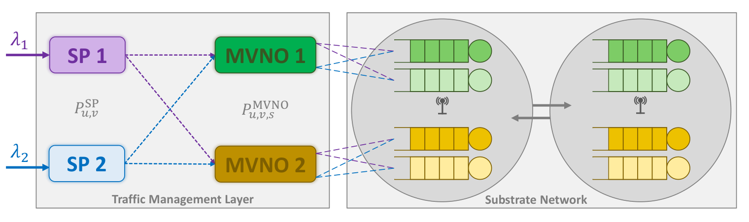
We consider each slice $s\in\mathcal{S}$ as a queue where data flows are customers and channels are servers. Then hereafter, we will use the terms slice and queue interchangeably. Customers from SP $u$ arrive at queue $s$ with rate $\lambda_{s,u}$ as a Poisson process and stay in queue until they receive service, i.e., being completely transmitted on one of $Q_{s}$ channels of the corresponding slice. The service time for each flow depends on its number of bits and wireless link capacity. Therefore, regarding interference coupling among slices and other assumptions, we consider a negative exponential distribution with variable rates. This means that we have a network of queues with service rate for each queue depending on the state of the other queues (i.e., the existing status of each channel) in the network. If the number of arrived customers is more than the existing servers, extra customers are buffered until we have a total of $Q^{\mathrm{max}}_{s}$ customers in the queue. If the buffer capacity is full, newly arrived customers would be blocked. Accordingly, in the entire system, we would have a network of queues where each one has a standard $M/M(n)/Q_{s}/Q^{\mathrm{max}}_{s}$ model. Since the state of each queue depends on the state of the whole network, we propose a state-dependent queueing network to model our system.

We say $s,s^{\prime}\in\mathcal{S}$ interact with each other, when they either have an overlapped frequency range or there exists at least one slice $s^{\prime\prime}\in\mathcal{S}$ that has some overlapped distinct frequency ranges with both $s$ and $s^{\prime}$. For example, in Fig. 2, slices $s=7$ and $s=8$ interact with each other because they both have overlapped frequency range with $s=12$. Keeping this in mind, one can partition $\mathcal{S}$ into disjoint subsets where queues in each subset interact with each other but not with queues in other subsets. Then, queues in each subset can be analyzed independently. Without loss of generality, we assume that all queues in $\mathcal{S}$ interact with each other.

Now consider a two-part and non-negative vector $\mathbf{n}=(\mathbf{n}_{\mathrm{LH}},\mathbf{n}_{\mathrm{RH}})$ of the state space $\mathbb{N}_{\mathbf{n}}$ as the network state vector where $\mathbf{n}_{\mathrm{LH}}$ and $\mathbf{n}_{\mathrm{RH}}$ are the left-hand and the right-hand parts with equal size $|\mathcal{S}|$. For each queue $s\in\mathcal{S}$, the elements $\mathbf{n}_{\mathrm{RH}}(s)$ and $\mathbf{n}_{\mathrm{LH}}(s)$, respectively, represent the number of customers and the remaining buffer capacity and therefore we have $\mathbf{n}_{\mathrm{LH}}(s)+\mathbf{n}_{\mathrm{RH}}(s)=Q^{\mathrm{max}}_{s}$. Also consider a similar two-part and non-negative vector $\mathbf{a}=(\mathbf{a}_{\mathrm{LH}},\mathbf{a}_{\mathrm{RH}})$ of the state space $\mathbb{N}_{\mathbf{a}}$ as the movement vector where for each queue $s\in\mathcal{S}$, the elements $\mathbf{a}_{\mathrm{RH}}(s)$ and $\mathbf{a}_{\mathrm{LH}}(s)$, respectively, represent the number of departures from and arrivals to $s$. Regarding the continuous time dynamic in our scenario only single movements are possible at each time. Therefore, for all vectors $\mathbf{a}$, the first norm is equal to one, i.e., $\lVert\mathbf{a}\rVert_{1}=1$. As a numerical example, for slicing configuration shown in Fig. 2 with $|\mathcal{S}|=12$, following vectors correspond to arrivals at queue $s=1$ when there are no customers in the network and each queue has a unity-size buffer (i.e., $Q^{\mathrm{max}}_{s}=Q_{s}+1$)

For each possible pair of $(\mathbf{n},\mathbf{a})$ vectors, we define $\xi(\mathbf{n},\mathbf{a})$ as the rate of leaving the state $\mathbf{n}$ through the movement $\mathbf{a}$. Vector $\mathbf{a}$, then, transforms into another vector $\mathbf{a}^{\prime}$ with probability $r(\mathbf{a},\mathbf{a}^{\prime})$ which changes the network state from $\mathbf{n}$ to $\mathbf{n}^{\prime}$. If $\mathbf{a}$ corresponds to an arrival to $s$, $\mathbf{a}^{\prime}$ corresponds to a departure from $s$, and vice versa. We define $\langle\mathbf{n},\mathbf{a}\rangle$ as the set of all pairs of $(\mathbf{n},\mathbf{a})$ that can transform into each other, i.e., $\mathbf{n}-\mathbf{a}=\mathbf{n}^{\prime}-\mathbf{a}^{\prime}$. In the previous example, vector $\mathbf{a}$ transforms into $\mathbf{a}^{\prime}=(0,0,0,0,0,0,0,0,0,0,0,0,1,0,0,0,0,0,0,0,0,0,0,0)$ with $r(\mathbf{a},\mathbf{a}^{\prime})=1$ changing the network state from $\mathbf{n}$ to $\mathbf{n}^{\prime}=(3,2,2,4,4,2,4,2,4,2,4,2,1,0,0,0,0,0,0,0,0,0,0,0)$. Obviously, in our model at each $\langle\mathbf{n},\mathbf{a}\rangle$ just two members exist. We also define $\pi(\mathbf{n})$ as the network steady-state probability distribution, i.e., the normalized network stationary measure. Now we use the following theorem from [29].

In general, definition of $P_{u,v,s}^{\mathrm{MVNO}}$ implies that each slice can serve customers from multiple SPs. But in this technical report, we assume $P_{u,v,s}^{\mathrm{MVNO}}$ value is such that slice $s\in\mathcal{S}$ at each time has only customers from a single SP $u$. This assumption is only for the sake of simplicity in formulations and can be relaxed by defining multiple new states within each slice corresponding to each SP. We would try to keep the formulation general, but we may occasionally use the notation $u_{s}$ to remind that $u$ depends on $s$. If we name the customers from each SP a class of customers, then the latter assumption means that we consider queues with a single class of customers. Note that the terms type of service and class of customer refer to two separate concepts, and there can be SPs that offer the same type of service. Therefore, for queue $s$ which has only customers from SP $u$, we define $\Lambda_{s,u}$ and $\mathrm{M}_{s,u}$ as the state-dependent arrival and service rates considering that $\mathrm{M}_{s,u}$, due to the coupled interference, is dependent on the network state, i.e., right-hand part $\mathbf{n}_{\mathrm{RH}}$, while $\Lambda_{s,u}$ is only dependent on the state of $s$, i.e., $\mathbf{n}_{\mathrm{RH}}(s)$. Now if we define functions $\Phi$ and $\Psi$ in a way that for each $s\in\mathcal{S}$ we have

then as a corollary of Theorem 1, $\Phi(\mathbf{n})$ is a stationary measure of the network. For this purpose, we present the following proposition.

In proposition 1, $\delta(.)$ is the Dirac delta function and $\mathbf{e}(\mathbf{x})$ is a two-part vector-valued function indicating whether there has been a movement in each queue or not and we have

where the left-hand part $\mathbf{0}_{\mathrm{LH}}$ is a zero vector with size $|\mathcal{S}|$ and the right-hand part $\mathbf{e}_{\mathrm{RH}}(\mathbf{x})=(e_{s})_{s\in\mathcal{S}}$ is a vector with size $|\mathcal{S}|$ and for element $e_{s}$ we have

Finally, notation $[\Phi_{2}(\mathbf{x})]_{\mathbf{x}\rightarrow\mathbf{x}+\mathbf{e}(\mathbf{x})}$ implies that one must determine $\Phi_{2}(\mathbf{x})$ first and then substitute all values of $\mathbf{x}$ with $\mathbf{x}+\mathbf{e}(\mathbf{x})$. The general idea here is to use the function $\mathbf{e}(\mathbf{x})$ to model perfectly all departure movements (but not the arrival movements) in (11) since a distinction between arrival and departure movements exists in (9). We explain this matter in the sequel.

To determine $\mathrm{M}_{s,u}(\mathbf{n}_{\mathrm{RH}})$, we need to consider that for each realization of $\mathbf{n}_{\mathrm{RH}}$, multiple channel allocations are possible resulting in multiple values for $\mathbf{\Delta}_{s,q}$ (interference vector corresponding to $(s,q)$). By averaging $C^{-1}_{s,q,u}(\mathbf{\Delta}_{s,q})$ (see (4)) over all possible values of $\mathbf{\Delta}_{s,q}$ we have

where $\mathrm{Pr}(\mathbf{\Delta}_{s,q})$ is the probability that the interference vector $\mathbf{\Delta}_{s,q}$ occurs. MVNOs can assign flows to vacant channels with different policies leading to different $\mathrm{Pr}(\mathbf{\Delta}_{s,q})$. In the case of random and independent channel allocation policy in all queues, we have

where $\hat{\mathcal{N}}_{s,q}=\{s^{\prime}|\exists q^{\prime},(s^{\prime},q^{\prime})\in\mathcal{N}_{s,q}\}$ is the set of slices which have frequency overlap with $(s,q)$ and $\mathbf{\Delta}_{s,q,s^{\prime}}$ is a sub-vector of $\mathbf{\Delta}_{s,q}$ corresponding to the interference from channels of slice $s^{\prime}$, and we have

where $\dim(.)$ and $\left\lVert.\right\rVert_{1}$, respectively, represent the dimension and the first norm of a vector. In justifying (16), it is worth noting that it is possible that more than one channel of a typical slice $s^{\prime}$ have frequency overlap with $(s,q)$.

Since the slices are arbitrary and in general, frequency range overlaps between two slices are asymmetric, channels of a single slice may have different average wireless link capacities indicated by $C_{s,q,u}(\mathbf{n}_{\mathrm{RH}})$ in (14). In terms of queueing theory, this means that we have queues with heterogeneous servers with varying service rates, which are complex to analyze. Therefore, for simplicity, we study an equivalent homogeneous queue with a total service rate equal to that of the heterogeneous queue. In other words, the service rate of each server in equivalent queue is the average of the heterogeneous queue service rates. For this purpose, in each state $\mathbf{n}_{\mathrm{RH}}$, considering a tagged flow that is assigned to arbitrary channel $q$ of slice $s$ and averaging $C_{s,q,u}(\mathbf{n}_{\mathrm{RH}})$ over all channels of slice $s$, we have

as the wireless link capacity for each channel in the equivalent homogeneous slice (queue), where $\mathrm{Pr}(q)$ is the probability that channel $q$ is assigned to a transmitting tagged flow. In the case of uniformly random channel allocation scheme, we have $\mathrm{Pr}(q)=1/Q_{s}$. Afterwards, we can achieve the state-dependent service rate for SP $u$-customers by dividing the obtained wireless link capacity by the average number of bits of the flows as in the following:

where the term $\frac{C_{s,u}(\mathbf{n}_{\mathrm{RH}})}{\Omega_{u}}$ represents the rate of serving flows at each server of queue $s$ and the term $\min(\mathbf{n}_{\mathrm{RH}}(s),Q_{s})$ implies that the service rate for queue $s$ increases as the number of customers $\mathbf{n}_{\mathrm{RH}}(s)$ increases until we have $Q_{s}$ customers or more, in which case, all servers are busy. When there are zero customers in a queue, the service rate is meaningless. Therefore, in order to neutralize the effect of $\mathrm{M}_{s,u}(\mathbf{n}_{\mathrm{RH}})$ in (10) and (11), we define $\mathrm{M}_{s,u}(\mathbf{n}_{\mathrm{RH}})=1$ in all such states.

So far and for a known network state vector $\mathbf{n}$, service rate $\mathrm{M}_{s,u}(\mathbf{n}_{\mathrm{RH}})$ has been obtained by multiple averaging over $C_{s,q,u}(\mathbf{\Delta}_{s,q})$, regarding the fact that in each network state, channel allocation for each slice is random and independent of the state of other slices. However, when investigating the steady-state probability distribution for a specific queue, the coupling effect among slices is a burden. In fact, to achieve the steady-state probability distribution, one must know the service rate for all states of queue, but, as indicated in $\mathrm{M}_{s,u}(\mathbf{n}_{\mathrm{RH}})$, service rate is a function of the state of other network queues. Thus, we need to solve the equations recursively.

We define state-dependent arrival rate as

Obviously, due to the consideration of blocking, when there are $Q^{\mathrm{max}}_{s}$ customers in a queue, the arrival rate to the queue is zero.

The defined $\Phi$ and $\Psi$ do not satisfy (19) perfectly. In fact, by substituting state-dependent rates defined by (18) and (19) in (10) and (11), one can investigate that (9) will have the following form

where $\beta_{\mathbf{n},\mathbf{a}}$ is a coefficient showing up due to $\Phi$ and $\Psi$ imperfection when the pair $(\mathbf{n},\mathbf{a})$ corresponds to a permitted arrival.

For arrivals to slice $s\in\mathcal{S}$ with $0\leq\mathbf{n}_{\mathrm{RH}}(s)<Q^{\mathrm{max}}_{s}$ and from (10) and (11) we obtain

where $\mathbf{1}_{s}$ is a vector with size $|\mathcal{S}|$ that its $s\text{-th}$ element is equal to one and the rest are equal to zero.

To neutralize the effect of $\beta_{\mathbf{n},\mathbf{a}}$, a solution is to introduce a modified state-dependent arrival rate $\hat{\Lambda}_{s,u}(\mathbf{n}_{\mathrm{RH}}(s))$ such that $\hat{\Lambda}_{s,u}(\mathbf{n}_{\mathrm{RH}}(s))\beta_{\mathbf{n},\mathbf{a}}\cong\Lambda_{s,u}(\mathbf{n}_{\mathrm{RH}}(s))$. Therefore, we define

where $\hat{\beta}_{s,\mathbf{n}_{\mathrm{RH}}(s)}$ is the modification factor. Hence, for all pairs of $(\mathbf{n},\mathbf{a})$ that correspond to an arrival to slice $s\in\mathcal{S}$ when it has $\mathbf{n}_{\mathrm{RH}}(s)$ customers, we can approximate (9) with (20) by choosing $\hat{\beta}_{s,\mathbf{n}_{\mathrm{RH}}(s)}$ so that $\lambda_{s,u}\frac{\beta_{\mathbf{n},\mathbf{a}}}{\hat{\beta}_{s,\mathbf{n}_{\mathrm{RH}}(s)}}$ has the least weighted squared error with respect to $\lambda_{s,u}$. In other words, to find the value of $\hat{\beta}_{s,\mathbf{n}_{\mathrm{RH}}(s)}$ for each $s\in\mathcal{S}$ and $0\leq\mathbf{n}_{\mathrm{RH}}(s)\textless Q^{\mathrm{max}}_{s}$, we have

where $\mathbf{x}$ is a variable vector similar to $\mathbf{n}$ and

is the normalized weight for state $\mathbf{x}$ as $\Phi(\mathbf{x})$ is a stationary measure of the network according to Theorem 1.

Since $\Phi(\mathbf{x})$ is dependent on $\hat{\beta}_{s,\mathbf{n}_{\mathrm{RH}}(s)}$ and vice versa, an iterative approach can be used to obtain $\Phi(\mathbf{x})$ as stated in Algorithm 1. For the proof please see Appendix B. To make reading easier, for the rest of the technical report, we represent the condition under sigma in (23) as $\mathrm{COND}(\mathbf{x},\mathbf{a})=\{\mathbf{x}\in\mathbb{N}_{\mathbf{n}},\mathbf{a}\in\mathbb{N}_{\mathbf{a}},\mathbf{a}_{\mathrm{LH}}(s)=1,\mathbf{x}_{\mathrm{RH}}(s)=\mathbf{n}_{\mathrm{RH}}(s)\}$.

For each network state $\mathbf{n}$, the obtained $\Phi(\mathbf{n})$ using Algorithm 1 is an approximate stationary measure of the network. The accuracy of this approximation depends on the weighted squared error in (23) which is related to three factors: the number of terms in summation, the weights $\hat{\Phi}_{s,\mathbf{n}_{\mathrm{RH}}(s)}(\mathbf{x})$ and the values of $\beta_{\mathbf{x},\mathbf{a}}$.

An increase in the number of possible network states means more possible pairs of $(\mathbf{x},\mathbf{a})$ in (23), leading to larger error value. The value of $\hat{\Phi}_{s,\mathbf{n}_{\mathrm{RH}}(s)}(\mathbf{x})$ can vary depending on the network traffic as it is a normalized stationary measure of the network. In light traffic, the weights for states with a low number of customers are dominant and other weights are almost negligible. In contrast, in heavy traffic, the weights for states with a large number of customers are dominant and other weights are almost negligible. In other words, for light and heavy traffic, the number of terms in summation (23) is fewer than the one in moderate traffic and therefore, the error value is less. Our numerical results confirm this matter.

To investigate the third factor, if we call $\hat{\beta}^{*}_{s,\mathbf{n}_{\mathrm{RH}}(s)}$ as the value that has been obtained from the last iteration of Algorithm 1, we can calculate the minimum cost. For arrivals to slice $s\in\mathcal{S}$ with $0\leq\mathbf{n}_{\mathrm{RH}}(s)\textless Q^{\mathrm{max}}_{s}$, by substituting $\hat{\beta}^{*}_{s,\mathbf{n}_{\mathrm{RH}}(s)}$ into (23) we have

where the symbols $\mathrm{E}[\beta_{\mathbf{x},\mathbf{a}}]=\sum_{\mathrm{COND}(\mathbf{x},\mathbf{a})}\hat{\Phi}_{s,\mathbf{n}_{\mathrm{RH}}(s)}(\mathbf{x})\beta_{\mathbf{x},\mathbf{a}}$ and $\mathrm{Var}[\beta_{\mathbf{x},\mathbf{a}}]=\mathrm{E}[\beta^{2}_{\mathbf{x},\mathbf{a}}]-\mathrm{E}^{2}[\beta_{\mathbf{x},\mathbf{a}}]$, respectively, represent the expectation and the variance. Consequently, any factor that increases the ratio between $\mathrm{Var}[\beta_{\mathbf{x},\mathbf{a}}]$ and $\mathrm{E}[\beta^{2}_{\mathbf{x},\mathbf{a}}]$, increases the weighted squared error in (23).

We define $\pi_{s}$ as the steady-state probability distribution for slice $s$ where $\pi_{s}(n)$ indicates the steady-state probability distribution of $n$ customers being present at queue $s$ and we have

We also define the blocking probability $P^{B}_{s}$ as the probability of customers arriving at queue $s$ being blocked and we have

We define $T_{s,u}$ as the throughput for SP $u$-users in slice $s$ and we have

We also define $D_{s,u}$ as the average total delay for SP $u$-users in slice $s$. Using the Little’s law we have

where the numerator indicates the average number of SP $u$-users in queue $s$ and the denominator indicates the rate of SP $u$-users admitted in queue $s$.

For each customer entering queue $s$, its total delay consists of sojourn time in buffer and service time. We define $D^{\mathrm{SJ}}_{s,u}$ and $D^{\mathrm{SV}}_{s,u}$, respectively, as the average sojourn and service time for SP $u$-users in queue $s$. With an approach similar to (28) we have

where the numerators, respectively, indicate the average number of SP $u$-users in buffer and servers of queue $s$, and the denominators, respectively, indicate the rate of SP $u$-users entering buffer and servers of queue $s$. One can verify that, for SP $u$-users in queue $s$, the equation $D_{s,u}=D^{\mathrm{SJ}}_{s,u}+D^{\mathrm{SV}}_{s,u}$ holds as expected.

Regardless of slice and cell, each MVNO has to serve SP $u$-users based on an SLA in the entire network. We define $T^{\mathrm{MVNO}}_{u,v}$ as the network throughput for SP $u$-users being served by MVNO $v$ and we have

Smillar to the slice delay, we define $D^{\mathrm{MVNO}}_{u,v}$, $D^{\mathrm{MVNO,SJ}}_{u,v}$ and $D^{\mathrm{MVNO,SV}}_{u,v}$, respectively, as the network total delay, network sojourn time and network service time for SP $u$-users being served by MVNO $v$ and we have

and the equation $D^{\mathrm{MVNO}}_{u,v}=D^{\mathrm{MVNO,SJ}}_{u,v}+D^{\mathrm{MVNO,SV}}_{u,v}$ holds.

We already stated the importance of isolation among slices. To quantify and compare isolation level in the network, here we propose some metrics. Suppose that the isolation for slices that are allocated to SP $u$-users being served by MVNO $v$ is under investigation and another SP $u^{\prime}$-users traffic has been continuously increased from $\lambda_{u^{\prime}}$ to $\lambda_{u^{\prime}}+\Delta\lambda$. Since the network KPIs are functions of SP $u^{\prime}$-users traffic, a KPI versus interfering traffic curve can be obtained. Therefore, for network total delay, we can define average of delay deviation (ADD) and variance of delay deviation (VDD) as

References

- [1] 5GPPP, “5GPPP architecture working group; view on 5G architecture,” October 2021, version 4.0. [Online]. Available: https://5g-ppp.eu/wp-content/uploads/2021/11/Architecture-WP-V4.0-final.pdf
- [2] Ericsson, “Ericsson mobility report,” November 2021. [Online]. Available: https://www.ericsson.com/4ad7e9/assets/local/reports-papers/mobility-report/documents/2021/ericsson-mobility-report-november-2021.pdf
- [3] C. Liang and F. R. Yu, “Wireless network virtualization: A survey, some research issues and challenges,” IEEE Commun. Surveys Tuts., vol. 17, no. 1, pp. 358–380, 2014.
- [4] I. Afolabi, T. Taleb, K. Samdanis, A. Ksentini, and H. Flinck, “Network slicing and softwarization: A survey on principles, enabling technologies, and solutions,” IEEE Commun. Surveys Tuts., vol. 20, no. 3, pp. 2429–2453, 2018.
- [5] 3GPP, “5G; NR; physical layer procedures for data,” April 2021, 3GPP TS 38.214 version 16.5.0 Release 16. [Online]. Available: https://www.etsi.org/deliver/etsi_ts/138200_138299/138214/16.05.00_60/ts_138214v160500p.pdf
- [6] M. Richart, J. Baliosian, J. Serrat, and J.-L. Gorricho, “Resource slicing in virtual wireless networks: A survey,” IEEE Trans. Netw. Service Manag., vol. 13, no. 3, pp. 462–476, 2016.
- [7] R. Su et al., “Resource allocation for network slicing in 5g telecommunication networks: A survey of principles and models,” IEEE Netw., vol. 33, no. 6, pp. 172–179, 2019.
- [8] Y. Azimi, S. Yousefi, H. Kalbkhani, and T. Kunz, “Energy-efficient deep reinforcement learning assisted resource allocation for 5g-RAN slicing,” IEEE Trans. Veh. Technol., pp. 856–871, 2021.
- [9] A. J. Gonzalez et al., “The isolation concept in the 5g network slicing,” in Proc. Eur. Conf. Netw. Commun. (EuCNC), 2020.
- [10] D. Marabissi and R. Fantacci, “Highly flexible ran slicing approach to manage isolation, priority, efficiency,” IEEE Access, vol. 7, pp. 97 130–97 142, 2019.
- [11] S. D’Oro, L. Bonati, F. Restuccia, and T. Melodia, “Coordinated 5g network slicing: How constructive interference can boost network throughput,” IEEE/ACM Trans. Netw., vol. 29, no. 4, pp. 1881–1894, aug 2021.
- [12] M. Zambianco and G. Verticale, “Interference minimization in 5g physical-layer network slicing,” IEEE Trans. Commun., vol. 68, no. 7, pp. 4554–4564, jul 2020.
- [13] S. D’Oro, F. Restuccia, A. Talamonti, and T. Melodia, “The slice is served: Enforcing radio access network slicing in virtualized 5g systems,” in Proc. IEEE INFOCOM, 2019.
- [14] S. Zarandi and H. Tabassum, “Delay minimization in sliced multi-cell mobile edge computing (MEC) systems,” IEEE Commun. Lett., vol. 25, no. 6, pp. 1964–1968, jun 2021.
- [15] O. Al-Khatib, W. Hardjawana, and B. Vucetic, “Wireless networks virtualisation: Traffic modeling and spectrum sharing,” in Proc. IEEE Int. Conf. Commun. (ICC), 2015.
- [16] ——, “Spectrum sharing in multi-tenant 5g cellular networks: Modeling and planning,” IEEE Access, vol. 7, pp. 1602–1616, 2019.
- [17] L. Feng, Y. Zi, W. Li, F. Zhou, P. Yu, and M. Kadoch, “Dynamic resource allocation with RAN slicing and scheduling for uRLLC and eMBB hybrid services,” IEEE Access, vol. 8, pp. 34 538–34 551, 2020.
- [18] B. Han, V. Sciancalepore, D. Feng, X. Costa-Perez, and H. D. Schotten, “A utility-driven multi-queue admission control solution for network slicing,” in Proc. IEEE INFOCOM, 2019, pp. 55–63.
- [19] B. Han, V. Sciancalepore, X. Costa-Pérez, D. Feng, and H. D. Schotten, “Multiservice-based network slicing orchestration with impatient tenants,” IEEE Trans. Wireless Commun., vol. 19, no. 7, pp. 5010–5024, 2020.
- [20] V. N. Ha, T. T. Nguyen, L. B. Le, and J.-F. Frigon, “Admission control and network slicing for multi-numerology 5g wireless networks,” IEEE Netw. Lett., vol. 2, no. 1, pp. 5–9, 2020.
- [21] H. Klessig, D. Öhmann, A. J. Fehske, and G. P. Fettweis, “A performance evaluation framework for interference-coupled cellular data networks,” IEEE Trans. Wireless Commun., vol. 15, no. 2, pp. 938–950, 2016.
- [22] H. Klessig, A. Fehske, and G. Fettweis, “Admission control in interference-coupled wireless data networks: A queuing theory-based network model,” in Proc. 12th Int. Symp. Model. Optim. Mobile, Ad Hoc, Wireless Netw. (WiOpt), 2014, pp. 151–158.
- [23] D. Oehmann, A. J. Fehske, and G. P. Fettweis, “Non-stationary traffic conditions in transient flow level models for cellular networks,” in Proc. 20th Eur. Wireless Conf., 2014, pp. 1–6.
- [24] A. Fehske, H. Klessig, J. Voigt, and G. Fettweis, “Flow-level models for capacity planning and management in interference-coupled wireless data networks,” IEEE Commun. Mag., vol. 52, no. 2, pp. 164–171, 2014.
- [25] D. Öhmann, A. Fehske, and G. Fettweis, “Transient flow level models for interference-coupled cellular networks,” in Proc. 51st Annu. Allerton Conf. Commun., Control, Comput. (ALLERTON), 2013, pp. 723–730.
- [26] A. J. Fehske and G. P. Fettweis, “Aggregation of variables in load models for interference-coupled cellular data networks,” in Proc. IEEE Int. Conf. Commun. (ICC), 2012, pp. 5102–5107.
- [27] H. Klessig and G. Fettweis, “Impact of inter-cell interference on buffered video streaming startup delays,” in Proc. IEEE 82nd Veh. Technol. Conf. (VTC), Fall 2015, pp. 1–2.
- [28] P. Mogensen et al., “Lte capacity compared to the shannon bound,” in Proc. IEEE 65th Veh. Technol. Conf. (VTC), Spring 2007, pp. 1234–1238.
- [29] X. Chao, M. Miyazawa, and M. Pinedo, Queueing networks: Customers, signals and product form solutions. Chichester, England: Wiley, 1999.