2021

Three-dimensional (3D) integrated renal structures (IRS) segmentation is important in clinical practice. With the advancement of deep learning techniques, many powerful frameworks focusing on medical image segmentation are proposed. In this challenge, we utilized the nnU-Net framework, which is the state-of-the-art method for medical image segmentation. To reduce the outlier prediction for the tumor label, we combine contour regularization (CR) loss of the tumor label with Dice loss and cross-entropy loss to improve this phenomenon.

KiPA22 Report: U-Net with Contour Regularization for Renal Structures Segmentation

Kangqing Ye Email: yekangq@sjtu.edu.cn Affiliation: Shanghai Jiao Tong University, Shanghai, China Peng Liu Affiliation: Shanghai Jiao Tong University, Shanghai, China Xiaoyang Zou Affiliation: Shanghai Jiao Tong University, Shanghai, China Qin Zhou Affiliation: Shanghai Jiao Tong University, Shanghai, China Guoyan Zheng Affiliation: Shanghai Jiao Tong University, Shanghai, China

1 Introduction

Three-dimensional (3D) integrated renal structures (IRS) segmentation on computed tomography angiography (CTA) images plays an important role in laparoscopic partial nephrectomy (LPN) shao2011laparoscopic. With the advancement of deep learning techniques, various deep learning methods have proven effective for IRS segmentation he2021meta; he2020dense. Many successful algorithms are base on the U-Net architecture heller2021state. NnU-Net (no new U-Net) is a self-configuring method based on the U-Net architecture, which outperforms most specialized deep learning pipelines in 19 public international segmentation competition isensee2021nnu. Although nnU-Net can produce outstanding results, there are still some outlier predictions especially for the tumor label. We introduce contour regularization (CR) loss of the tumor label into our loss function to improve this phenomenon.

2 Method

2.1 Preprocessing

The intensity value of the origin images is clipped to the [0.5, 99.5] percentiles to avoid outliers.

2.2 Network

3D full resolution U-Net configuration of nnU-Net isensee2021nnu is chosen (Fig 1). The contracting path includes $5$ downsampling steps. Deep supervision is also used.

Refer to caption — Figure 1: The 3D U-Net architecture that is used in this work.

2.3 Loss function

We use the summation between Dice loss, cross-entropy loss and contour regularization loss. The baseline nnU-Net method, which do not use the contour regularization loss, produces many outlier predictions of the tumor label. Contour regularization loss constrains the continuity and connectivity to reduce the outlier predictions hu2021fully. Take bi-dimensional situation for example, let $p\in[0,1]^{H\times W}$ denote the predicted probability of each pixel to be the tumor label. The contour of prediction on position (i, j) is then defined as the largest probability variation surrounding,

\mathcal{C}_{d}\left(p_{i,j}\right)=\max_{\left(i_{1},j_{1}\right),\left(i_{2},j_{2}\right)\in\mathcal{W}_{d}(i,j)}\left\|p_{i_{1},j_{1}}-p_{i_{2},j_{2}}\right\|

(1)

where $\mathcal{W}_{d}(i,j)=\{i\pm k,j\pm l\mid k,l\in\{0\ldots d\}\}$ denotes the set of pixels around the point $(i,j)$ with radius $d$ . The contour could be implemented as following:

\mathcal{C}_{d}\left(p_{i,j}\right)=\max_{\begin{subarray}{c}\left(i_{c},j_{c}\right)\\ \in\mathcal{W}_{d}(i,j)\end{subarray}}p_{\left(i_{c},j_{c}\right)}-\min_{\begin{subarray}{c}\left(i_{c},j_{c}\right)\\ \in\mathcal{W}_{d}(i,j)\end{subarray}}p_{\left(i_{c},j_{c}\right)}=\mathcal{M}_{d}\left(p_{i,j}\right)+\mathcal{M}_{d}\left(-p_{i,j}\right)

(2)

where $\mathcal{M}_{d}$ is the max pooling operation with kernel size $2d+1$ .

Similarly, in the three-dimensional situation, the contour could be implemented as following:

\mathcal{C}_{d}\left(p_{i,j,k}\right)=\max_{\begin{subarray}{c}\left(i_{c},j_{c},k_{c}\right)\\ \in\mathcal{W}_{d}(i,j,k)\end{subarray}}p_{\left(i_{c},j_{c},k_{c}\right)}-\min_{\begin{subarray}{c}\left(i_{c},j_{c},k_{c}\right)\\ \in\mathcal{W}_{d}{(i,j,k)}\end{subarray}}p_{\left(i_{c},j_{c},k_{c}\right)}=\mathcal{M}_{d}\left(p_{i,j,k}\right)+\mathcal{M}_{d}\left(-p_{i,j,k}\right)

(3)

Therefore, the contour regularization loss can be represented as following:

	$\displaystyle\mathcal{L}_{CR}$	$\displaystyle=\left\\|\max_{n_{1},n_{2}\in\mathcal{W}_{d}(n)}\left\\|p_{t}^{n_{1}}-p_{t}^{n_{2}}\right\\|\right\\|_{2}$		(4)
		$\displaystyle=\left\\|\mathcal{M}_{d}\left(p_{i,j,k}\right)+\mathcal{M}_{d}\left(-p_{i,j,k}\right)\right\\|_{2}$		(4)

where $\left\|\cdot\right\|_{2}$ denotes $l_{2}$ -norm.

The whole loss function in our method is shown as below:

\mathcal{L}_{T}=\mathcal{L}_{Dice}+\mathcal{L}_{cross-entropy}+\alpha\mathcal{L}_{CR}

(5)

where parameter $\alpha$ adjusts the weight of contour regularization loss.

2.4 Post-processing

None.

3 Dataset and Evaluation Metrics

3.1 Dataset

•

Original images are unenhanced abdominal CT images (as .nii.gz files) from 130 patients, 70 for the training dataset, 30 for the closed testing dataset, and 30 for the opened testing dataset.
•

The target structures are: kidney-Abnormal organ, tumor-Multi-subtype lesion, renal Artery-Very-thin structure, renal Vein-Low-significant region.
•

In the competition phase, the model proposed in this article is trained on 70 cases in the provided training set. The provided results analysis is based on the 4-fold cross validation results.

3.2 Evaluation Metrics

•

DSC (Dice Similarity Coefficient)
•

HD (Hausdorff Distance)
•

AVD (Average Hausdorff Distance)

4 Implementation Details

4.1 Environments and requirements

The environments and requirements of our method is shown in Table 1.

Table 1: Environments and requirements.

OS	Ubuntu 16.04.6 LTS
CPU	Intel(R) Xeon(R) Silver 4110 CPU @ 2.10GHz
RAM	256G
GPU	Nvidia RTX2080Ti
CUDA version	11.1
Programming language	Python3.9
Deep learning framework	Pytorch(Torch 1.8.1, torchvision 0.9.1)
Specification of dependencies	nnU-Netisensee2021nnu

4.2 Training protocols

Our training approach closely follows the training method of the nnU-Net framework, which is shown in Table 2. We employ 4-fold cross validation strategy so that every fold has 17 or 18 validation cases.

Table 2: Training protocols.

Data augmentation methods	Rotations, scaling, brightness, contrast, gamma correction and mirroring
Patch sampling strategy	A third of the samples in a batch contain at least one randomly chosen foreground class isensee2021nnu.
Batch size	2
Patch size	$160\times 128\times 112$
Total epochs	1000
Optimizer	Stochastic gradient descent
Initial learning rate	0.01

5 Results

5.1 Quantitative results on validation set

Table 3 shows the quantitative results on the open test dataset.

Table 3: Quantitative results on validation set

\toprule	DSC(%)	HD(mm)	AVD(mm)
\midruleKidney	$95.63\pm 2.0$	$16.71\pm 14.1$	$0.60\pm 0.5$
Tumor	$88.76\pm 11.4$	$14.23\pm 20.1$	$1.51\pm 2.4$
Artery	$87.33\pm 4.9$	$21.44\pm 24.4$	$0.46\pm 0.6$
Vein	$84.85\pm 5.6$	$17.09\pm 19.0$	$0.89\pm 1.2$
\bottomrule

5.2 Visualization result

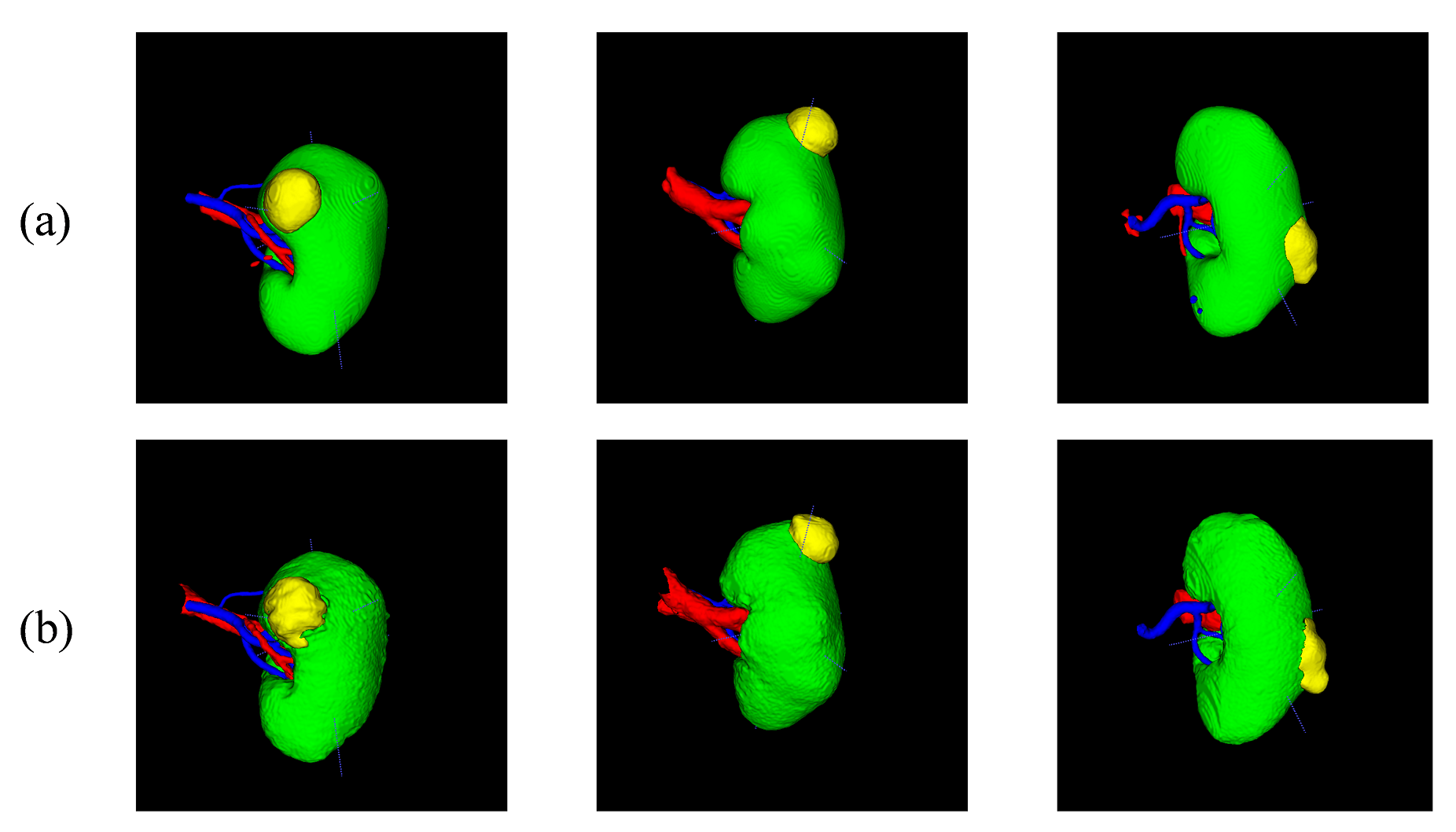
Figure 2 presents three example of validation set in training phase.

References

(1) Shao, P., Qin, C., Yin, C., Meng, X., Ju, X., Li, J., Lv, Q., Zhang, W., Xu, Z.: Laparoscopic partial nephrectomy with segmental renal artery clamping: technique and clinical outcomes. European urology 59(5), 849–855 (2011)
(2) He, Y., Yang, G., Yang, J., Ge, R., Kong, Y., Zhu, X., Zhang, S., Shao, P., Shu, H., Dillenseger, J.-L., et al.: Meta grayscale adaptive network for 3d integrated renal structures segmentation. Medical Image Analysis 71, 102055 (2021)
(3) He, Y., Yang, G., Yang, J., Chen, Y., Kong, Y., Wu, J., Tang, L., Zhu, X., Dillenseger, J.-L., Shao, P., et al.: Dense biased networks with deep priori anatomy and hard region adaptation: Semi-supervised learning for fine renal artery segmentation. Medical image analysis 63, 101722 (2020)
(4) Heller, N., Isensee, F., Maier-Hein, K.H., Hou, X., Xie, C., Li, F., Nan, Y., Mu, G., Lin, Z., Han, M., et al.: The state of the art in kidney and kidney tumor segmentation in contrast-enhanced ct imaging: Results of the kits19 challenge. Medical image analysis 67, 101821 (2021)
(5) Isensee, F., Jaeger, P.F., Kohl, S.A., Petersen, J., Maier-Hein, K.H.: nnu-net: a self-configuring method for deep learning-based biomedical image segmentation. Nature methods 18(2), 203–211 (2021)
(6) Hu, M., Song, T., Gu, Y., Luo, X., Chen, J., Chen, Y., Zhang, Y., Zhang, S.: Fully test-time adaptation for image segmentation. In: International Conference on Medical Image Computing and Computer-Assisted Intervention, pp. 251–260 (2021). Springer