Spin functional renormalization group for the quantum Heisenberg model
Abstract
We use our recently developed functional renormalization group (FRG) approach for quantum spin systems to investigate the phase diagram of the frustrated quantum Heisenberg model on a cubic lattice. From a simple truncation of the hierarchy of FRG flow equations for the irreducible spin-vertices which retains only static spin fluctuations and neglects the flow of the four-spin interaction, we can estimate the critical temperature with a similar accuracy as the numerically more expensive pseudofermion FRG. In the regime where the ground state exhibits either ferromagnetic or antiferromagnetic order, a more sophisticated truncation including the renormalization of the four-spin interaction as well as dynamic spin fluctuations reveals the underlying renormalization group fixed point and yields critical temperatures which deviate from the accepted values by at most .
I Introduction
Frustrated spin systems continue to be of great interest in modern condensed matter physics because they can exhibit intriguing complexity which can be explored experimentally and poses a challenge to theory Diep20. While in reduced dimensions spin systems can be investigated with the help of powerful numerical methods such as the density matrix renormalization group White92; Schollwoeck05, controlled methods for realistic three dimensional systems are not available. It is therefore important to develop approximate methods for studying frustrated spin systems in an unbiased way. A promising method is the functional renormalization group (FRG) Wetterich93; Berges02; Pawlowski07; Kopietz10; Metzner12; Dupuis21, which is one of the few unbiased quantitative methods for investigating the dominant instabilities of interacting fermions on a lattice Metzner12; Dupuis21; Hille20. Given the fact that with the help of Abrikosov’s pseudofermion representation of spin operators Abrikosov65 any spin Hamiltonian can be mapped onto an interacting fermion Hamiltonian acting on a projected Hilbert space, it is clear that the established FRG machinery for interacting fermions can also be applied to quantum spin systems. This strategy, called pseudofermion FRG, was pioneered by Reuther and Wölfle Reuther10 in 2010; since then it has has been used to investigate the phase diagrams and static correlation functions of many different spin models Reuther11; Reuther11a; Buessen16; Iqbal16; Baez2017; Rueck18; Thoenniss20; Kiese22; Ritter22. However, the pseudofermion FRG has some disadvantages: (1) the Hilbert space projection can only be implemented approximately, (2) the calculation of the spin dynamics has so far not been possible, (3) available truncations are not sufficient to obtain proper renormalization group fixed points and the associated critical behavior, and (4) explicit solutions of even severely truncated flow equations require heavy numerical calculations. At this point, we should mention that an alternative representation of the spin operators in terms of Majorana fermions Martin1959; Tsvelik1992 has recently been used to develop a pseudo-Majorana FRG Niggemann2021; Niggemann22, which does not suffer from the problem (1) and can also reproduce the non-trivial scaling characteristic for a proper renormalization group fixed point Niggemann22. However, the other problems mentioned above remain also for the pseudo-Majorana FRG. Motivated by the desire to avoid at least some of these problems, in Ref. [Krieg19] an alternative FRG approach to quantum spin systems has been proposed which does not rely on any representation of spin operators in terms of fermionic or bosonic auxiliary operators. The crucial insight of Ref. [Krieg19] is that the generating functional of the imaginary time ordered spin correlation functions satisfies an exact flow equation which can be directly obtained by differentiating the representation of as a trace of a time-ordered exponential over the physical Hilbert space of the spin systen. For recent applications of this spin FRG approach see Refs. [Tarasevych18; Goll19; Goll20; Tarasevych21; Tarasevych22; Rueckriegel22]; in particular, this approach has been used to calculate the dynamic structure factor of Heisenberg magnets at infinite temperature Tarasevych21, to investigate the critical spin dynamics of Heisenberg ferromagnets Tarasevych22, and to study dimerized spin systems Rueckriegel22.
In this work we use the spin FRG to investigate the phase diagram and the critical temperature of a frustrated quantum spin model in three dimensions. Specifically, we consider the Hamiltonian of the quantum Heisenberg model
| (1) |
where the spin operators are localized at the sites of a simple cubic lattice and denotes summation over all distinct pairs of -th nearest neighbor spins. This model has recently been used as a benchmark to test the accuracy of different implementations of the pseudofermion FRG Iqbal16; Kiese22; Ritter22. In this work we will apply our spin FRG approach to the model and compare the results to the pseudofermion FRG. Our main result is that the simplest possible truncation of the spin FRG produces results which are consistent with the numerically more expensive pseudofermion FRG. Moreover, using more sophisticated truncations of the spin FRG flow equations, we can obtain renormalization group fixed points, improve our estimates for the critical temperatures, and calculate the spin dynamics.
The rest of this work is organized as follows: In Sec. II we briefly discuss the classical zero temperature phase diagram of our model. In Sec. III, we investigate the effect of classical spin fluctuations on the critical temperature using simple static approximations of the spin FRG flow equations, with and without taking into account the renormalization of the four-spin interaction. We improve our static estimates in Sec. IV by including the effect of dynamic spin fluctuations due to the quantum dynamics of the spin operators. In Sec. V we summarize our main results and point out necessary modifications of our approach to deal with strongly frustrated spin systems. Finally, in four appendices we give additional technical details: in Appendix A we write down FRG flow equations in static approximation, Appendix B provides a discussion of the renormalization group flow and fixed point in the static approximation, while in Appendix C we derive initial conditions for the relevant dynamical five and six-point vertices. The last Appendix D investigates an alternative parametrization of the dynamic spin fluctuations which serves as an input for the FRG calculation of the thermodynamics and static correlation function.
II Classical phase diagram
In the classical limit where the spin operators are replaced by three-component vectors with length the ground state phase diagram can be obtained by minimizing the classical Hamiltonian subject to the constraints . The classical ground state energy of the model (1) on a cubic lattice can then be written as
| (2) |
where is the ordering wavevector and is the total number of lattice sites. For a simple cubic lattice the Fourier transform of the exchange couplings is
| (3) |
where we have introduced the normalized form factors
| (4a) | ||||
| (4b) | ||||
| (4c) | ||||
We measure wavevectors in units of the inverse lattice spacing. According to Ref. [Iqbal16], in the classical limit one of the following four ground states is realized in the model on a cubic lattice: antiferromagnet (AF) with ordering wavevector ; striped AF with (we call this “spaghetti order”); layered AF with (“lasagne order”); ferromagnet with . From the condition that the physical ground state minimizes we obtain the classical zero temperature phase diagram shown in Fig. 1.

At finite temperature the boundaries between the paramagnetic phase and the magnetically ordered phases can be obtained from the momentum-dependent static susceptibility . Assuming that the phase transition to the magnetically ordered phase is continuous, we can determine the phase boundaries from the condition that diverges at the transition to a magnetically ordered state with ordering wavevector . Within a simple mean-field approximation (see below) the static susceptibility is
| (5) |
where the Fourier transform of the exchange coupling is given in Eq. (3), and
| (6) |
is the first coefficient in the expansion of the Brillouin function
| (7) |
In this approximation the critical temperature for a transition to a state with magnetic ordering wavevector is given by the mean-field result
| (8) |
Because is the global minimum of , the magnetic order in the classical ground state can also be identified with the state with the highest critical temperature.
As a quantitative measure for the degree of frustration in the system, it is useful to consider the energy-dependent density of states
| (9) |
where the momentum sum is over the first Brillouin zone. In Figs. 2 and 3 we show a numerical evaluation of for for representative values of the exchange couplings.
The momentum of the state at the lower band edge determines the magnetic order in the classical ground state. If the ground state is separated by a large energy interval from the other candidate states the system is weakly frustrated, see Fig. 2. The corresponding points in the phase diagram shown in Fig. 1 are far away from any of the phase boundaries. On the other hand, if the exchange couplings are chosen such that the corresponding points in the phase diagram are at or close to phase boundaries, the state at the lower edge of the band is energetically very close to the other candidate states as illustrated in Fig. 3. Hence, the frustration is strong in these cases. Additionally, one can see that competing states have an enhanced density of states. In the extreme cases where several ground states are actually degenerate, we expect reduced critical temperatures and possibly spin-liquid behavior. In the following section we will investigate this possibility within a simple static truncation of the spin FRG flow equations.
III Static spin FRG
To go beyond the mean-field approximation, we use the spin FRG approach proposed in Ref. [Krieg19] and further developed in Refs. [Tarasevych18; Goll19; Goll20; Tarasevych21; Tarasevych22; Rueckriegel22]. For our purpose the hybrid approach developed in Ref. [Tarasevych21] (see also Appendix B of Ref. [Rueckriegel22]) is most convenient. Let us briefly outline the main ideas of this implementation of the spin FRG. First of all, we replace the bare exchange coupling by a deformed coupling parametrized by a continuous scale parameter . The deformation scheme is chosen such that the exchange coupling is sufficiently simple so that the correlation functions of the deformed system can be calculated exactly, whereas corresponds to the undeformed system. In this work we use two different deformation schemes: a simple interaction-switch Krieg19,
| (10) |
that linearly switches on the exchange couplings, and a Litim regulator Litim01; Rancon11a; Rancon11b; Rancon12b; Rancon14; Rueckriegel22
| (11) |
that gradually increases the bandwidth of the exchange couplings, where are the maximum (minimum) value of . In both schemes we have , such that the spin correlations at are site-diagonal and are determined by the dynamics of a single spin. The corresponding time-ordered correlation functions are highly non-trivial and can be obtained diagrammatically by means of the generalized Wick-theorem for spin operators developed by Vaks, Larkin, and Pikin Vaks68; Vaks68b, see also see also Ref. [Izyumov88]. Note that recently Goll19 a purely algebraic form of the generalized Wick theorem for spin operators has been derived which does not rely on the rather complicated diagrammatic rules introduced in Refs. [Vaks68; Vaks68b; Izyumov88]. As shown in Ref. [Krieg19], the deformed generating functional of the imaginary time-ordered spin correlation function satisfies a formally exact FRG flow equation. It follows that the subtracted Legendre transform of satisfies the usual Wetterich equation Wetterich93. Unfortunately, at the initial scale where the deformed exchange coupling vanishes, the Legendre transform does not exist due to the vanishing of dynamic two-spin correlations of an isolated spin Rancon14; Krieg19. For this reason the lattice FRG proposed by Machado and Dupuis Machado10 for classical spin systems cannot be straightforwardly generalized to quantum spin systems. In Ref. [Tarasevych21] we have solved this problem by decomposing spin fluctuations into static and dynamic components and performing a Legendre transformation only in the static sector. Dynamic fluctuations are treated differently by working with “hybrid vertices” which are interaction-irreducible in the dynamic sector. These vertices are generated by the hybrid functional introduced in Ref. [Tarasevych21], which depends on the static (classical) magnetization and on a dynamic auxiliary field that can be interpreted as the frequency-dependent part of an internal magnetic field generated by the exchange interaction.
In the paramagnetic phase, the scale-dependent static spin susceptibility can then be written as
| (12) |
where is the scale-dependent spin self-energy with initial condition
| (13) |
The mean-field result (5) corresponds to neglecting the flow of this self-energy. Assuming that a possible phase transition to a magnetically ordered state is continuous, the critical temperature can be determined from the condition that the spin susceptibility (12) at the ordering wavevector diverges at the end of the flow.
To go beyond the mean-field approximation, let us now consider the flow of the static spin self-energy . In this section we use the static approximation, where all vertices involving external legs with finite frequencies are neglected. Formally, this amounts to setting . Given the fact that finite-temperature critical behavior is completely determined by classical fluctuations, we expect that the static approximation is sufficient to obtain the fixed point of the renormalization group flow associated with a finite temperature phase transition. The spin self-energy defined via Eq. (12) then satisfies the flow equation
| (14) |
where the single-scale propagator is defined by
| (15) |
and the irreducible four-point vertex describes the interaction between four spins in the static limit. Note that the three-point vertex vanishes because we consider the paramagnetic phase where there is no spontaneous magnetization. With our deformation scheme where the deformed exchange interaction initially vanishes, the initial value of the four-point vertex is determined by the irreducible part of a rotationally invariant combination of four-spin correlation functions of an isolated spin in the static limit Goll19; Tarasevych21. In Appendix A we show that
| (16) |
where
| (17) |
is the third order coefficient in the Taylor expansion (7) of the Brillouin function.
III.1 Level-1 truncation
In the simplest level-1 truncation Metzner12 we approximate the four-point vertex by its initial value given in Eq. (16). A similar level-1 truncation of the hierarchy of FRG flow equations has been used to calculate the renormalization of impurity potentials in mesoscopic Luttinger liquids Meden02; Metzner12. The spin self-energy is then independent of the momentum and its flow equation (14) reduces to
| (18) |
which can be straightforwardly integrated numerically with the initial condition (13).
In Fig. 4 we show our numerical results for the inverse susceptibility at the end of the FRG flow as a function of the dimensionless temperature for three different sets of exchange couplings. Note that for the nearest neighbor exchange (, ) displayed in Fig. 4 (a), our flow equation (18) is independent of the sign of the nearest neighbor coupling . Therefore we obtain the same temperature dependence of the susceptibility for ferro- and antiferromagnets, which is only correct in the classical limit footnote_classical; Oitmaa04. Remedying this for finite requires the inclusion of dynamical quantum fluctuations, which will be addressed in Sec. IV.
Obviously, within the level-1 truncation used in this section the inverse susceptibility approaches zero only asymptotically for , implying a paramagnetic state at finite temperature. This is of course an artifact of the level-1 truncation, which neglects the renormalization of the four-point vertex. We show in Appendix B that a true fixed point of the renormalization group flow can only be obtained if the flow of the four-point vertex is taken into account. Nevertheless, the existence of a kink in the temperature dependence of the inverse susceptibility shown in Figs. 4 (a) and (b) suggests that a large part of the renormalization group flow in the level-1 truncation still “feels” the influence of an underlying critical fixed point for these parameters. We therefore estimate the critical temperature by the position of the associated maximum in the second derivative of the inverse susceptibility with respect to temperature. In Table 1, we have collected the critical temperatures obtained in this manner, using both deformation schemes discussed above, and compare them to the accepted benchmark values from quantum Monte-Carlo simulations Sandvik98; Troyer04; Iqbal16 and high-temperature expansions Oitmaa04.
| rel. error / | ||||||||||
|---|---|---|---|---|---|---|---|---|---|---|
| switch | Litim | benchmark | switch | Litim | ||||||
| 0 | 0.651 | 0.568 | 0.559 | 16.5 | 1.6 | |||||
| 0 | 0.651 | 0.568 | 0.629 | 3.5 | 9.7 | |||||
| 0 | 0.726 | 0.668 | 0.650 | 11.7 | 2.8 | |||||
| 0 | 0.726 | 0.668 | 0.684 | 6.1 | 2.3 | |||||
| 0 | 0.745 | 0.695 | 0.685 | 8.8 | 1.5 | |||||
| 0 | 0.745 | 0.695 | 0.702 | 6.1 | 1.0 | |||||
| 0.2 | 0.746 | 0.701 | 0.722 | 3.3 | 2.9 | |||||
| 0.4 | 0.782 | 0.753 | 0.768 | 1.8 | 2.0 | |||||
| 0.6 | 0.800 | 0.776 | 0.794 | 0.8 | 2.3 | |||||
| 0.8 | 0.807 | 0.787 | 0.808 | 0.1 | 2.6 | |||||
| 0 | 0.766 | 0.725 | 0.722 | 6.1 | 0.4 | |||||
The overall agreement is rather good, with the largest deviation for the nearest neighbor case, where the static approximation does not distinguish between ferro- and antiferromagnetic nearest-neighbor couplings.
Next, let us consider Fig. 4 (c) in more detail. For , , , the classical ground states with spaghetti-order [ and lasagne-order [] are degenerate at the mean-field level; see Figs. 1 and 3. For this specific set of parameters an older one-loop pseudofermion FRG study Iqbal16 reported evidence for a paramagnetic ground state, whereas a more sophisticated multiloop pseudofermion FRG Ritter22 found that eventually the system exhibits spaghetti order (striped AF) at low temperatures. As our spin FRG results do not exhibit any kink as a function of temperature for these parameters, our calculation suggests a paramagnetic ground state, in agreement with the older pseudofermion FRG results by Iqbal et al. Iqbal16.
We conclude that, at least for the three-dimensional model on a cubic lattice, a simple static level-1 truncation of the spin FRG flow equations (where the frequency-dependence of all vertices as well as the renormalization of the four-point vertex are neglected) gives results for the critical temperature of similar accuracy as the numerically more expensive multiloop pseudofermion FRG. On the other hand, the fact that our static level-1 truncation of the spin FRG flow equations does not reproduce the magnetic order found in a recent multiloop pseudofermion FRG Ritter22 in a regime where classically the system exhibits degenerate ground states might indicate that in this regime our level-1 truncation possibly tends to over-estimate the role of spin fluctuations.
III.2 Level-2 truncation
The absence of a sharp phase transition in the level-1 truncation is due to the fact that within this truncation the flow of the four-point vertex is neglected. As shown in Appendix B, this leads to a runaway flow of the rescaled couplings. In the parameter regime where the classical ground state is not degenerate, it is however straightforward to recover a fixed point within our spin FRG approach in a level-2 truncation which takes the renormalization of the four-spin interaction into account. Note that within the pseudofermion FRG the four-spin interaction is encoded in the fermionic eight-point vertex which is usually neglected Reuther10; Reuther11; Reuther11a; Buessen16; Iqbal16; Baez2017; Rueck18; Thoenniss20; Kiese22; Ritter22. On the other hand, within the pseudo-Majorana FRG Niggemann2021; Niggemann22 the renormalization of the four-spin interaction can at least partially be taken into account due to an operator identity relating products involving different numbers of Majorana fermions Mao03; Shnirman03.
The FRG flow equation for the momentum-dependent static four-point vertex that determines the flow of the spin self-energy via Eq. (14) is given in Appendix A. In practice, additional approximations are necessary. For simplicity, let us focus here on non-degenerate classical ground states. Then we can adopt the truncation strategy of Ref. [Krieg19], where the critical temperature of the three-dimensional Ising model has been obtained to an accuracy of about using a truncation where the momentum-dependence of the renormalized four-point vertex is neglected and the six-point vertex is approximated by its initial value. A similar truncation strategy for the Heisenberg model leads to the following flow equation for the renormalized four-point vertex :
| (19) |
where
| (20) |
is the initial value of the longitudinal six-point vertex defined in Appendix A. Here and are defined in Eqs. (6) and (17) respectively, and
| (21) |
is the fifth-order coefficient in the expansion (7) of the Brillouin function. The corresponding flow of the static self-energy is obtained by replacing in Eq. (18),
| (22) |
Our numerical results for the inverse susceptibility and the four-point vertex at the end of the flow are displayed in Fig. 5 as a function of the dimensionless temperature .
In contrast to the level-1 truncation, the inverse susceptibility as well as the four-point vertex now vanish at a critical temperature , signaling a phase transition. We explicitly show in Appendix B how this phase transition is governed by the Wilson-Fisher fixed point for the nearest-neighbor Heisenberg magnet. The associated values for are listed in Table 2.
| rel. error / | ||||||||||
|---|---|---|---|---|---|---|---|---|---|---|
| switch | Litim | benchmark | switch | Litim | ||||||
| 0 | 0.578 | 0.525 | 0.559 | 3.4 | 6.1 | |||||
| 0 | 0.578 | 0.525 | 0.629 | 8.1 | 16.5 | |||||
| 0 | 0.672 | 0.625 | 0.650 | 3.4 | 3.8 | |||||
| 0 | 0.672 | 0.625 | 0.684 | 1.8 | 8.6 | |||||
| 0 | 0.701 | 0.658 | 0.685 | 2.3 | 3.9 | |||||
| 0 | 0.701 | 0.658 | 0.702 | 0.1 | 6.3 | |||||
| 0.2 | 0.712 | 0.676 | 0.722 | 1.4 | 6.4 | |||||
| 0.4 | 0.768 | 0.740 | 0.768 | 0.0 | 3.7 | |||||
| 0.6 | 0.795 | 0.771 | 0.794 | 0.1 | 2.9 | |||||
| 0.8 | 0.808 | 0.787 | 0.808 | 0.0 | 2.6 | |||||
| 0 | 0.736 | 0.700 | 0.722 | 1.9 | 3.0 | |||||
Note the striking agreement with the accepted benchmark values, in particular for the interaction-switch deformation scheme. In contrast, the tendency of the Litim scheme to underestimate the value of even worsens compared to the level-1 results displayed in Table 1. A possible explanation for the better performance of the interaction-switch deformation for the calculation of is that with this deformation scheme our truncation is perturbatively controlled in , which is small as long as the deformation parameter is sufficiently small or the temperature is large. Note furthermore that the interaction-switch deformation does not modify the momentum dependence of , in contrast to the Litim cutoff. We also remark that the accuracy of the static truncation quickly increases with increasing , reflecting the decreasing relevance of dynamic fluctuations in this case; see the following Sec. IV.
IV Including dynamic spin fluctuations
While the static approximation of the previous Sec. III already yields reasonable results for for various quantum magnets, it fails to distinguish between the nearest-neighbor ferro- and antiferromagnets at finite . To remedy this deficiency, we include also dynamic fluctuations at finite frequencies in this section. Within the hybrid approach developed in Ref. [Tarasevych21], such quantum fluctuations are described by dynamic vertices involving at least one finite-frequency leg associated with the auxiliary field that represents the dynamic internal exchange field. To leading order, these vertices can be approximated by their initial values describing the dynamic correlations of an isolated spin. The leading dynamic modification of the flow of the static spin self-energy is then given by the diagram shown in Fig. 6 (a), where the green triangle represents the dynamic chiral three-point vertex Tarasevych21,
| (23) |
where the superscripts denote the type of external legs: represents a static fluctuation of the longitudinal magnetic field, while and represent the spherical components of the dynamic exchange field . Note that in a Cartesian basis this vertex is determined by the chiral on-site expectation value . For a non-degenerate ground state, we should then evaluate the flow of the static self energy and the static four-point vertex at the ordering wavevector . In this case the flow equation (22) for the static self-energy is replaced by
| (24) |
where the dynamical propagator and its single-scale counterpart are defined by
| (25a) | ||||
| (25b) | ||||
Here, is the irreducible dynamic spin-susceptibility Tarasevych21. Note that in the classical limit, the contribution of dynamic spin fluctuations to the flow of vanishes as after appropriate rescaling footnote_classical. Hence, the classical limit corresponds to the static truncation of the flow equations, whereas the dynamical terms describe the effect of quantum fluctuations at finite .
For consistency, we should also take the effect of chiral dynamic fluctuations in the flow of the four-point vertex into account. Approximating the relevant higher-order dynamic vertices by their initial values, we find that the flow equation (19) for the static four-point vertex is modified as follows,
| (26) |
The frequency-dependent terms in Eq. (26) are shown diagrammatically in Fig. 6 (b).
As in Sec. III, there is no momentum transfer in the static part of the flow because is always a reciprocal lattice vector. For the explicit evaluation of the flow equation (26) of the static four-point vertex, we also need the initial values of the higher-order dynamic vertices. As shown in Appendix C the relevant initial values of the higher-order vertices are
| (27) | ||||
| (28) |
Also note that all four-point vertices with two legs at finite frequency, e.g. , are initially zero Tarasevych21 and therefore diagrams containing them do not contribute to the flow equations. To close the system of flow equations (24) and (26), we still need an expression for the dynamic irreducible susceptibility . In principle, we can also write down a flow equation for this function which has been derived in Ref. [Tarasevych21]. In this work, we instead opt to use the leading term in the high-temperature expansion,
| (29) |
which, for instance, can be obtained by iterating the flow of up to second order in Kriegthesis. Such a high-temperature approximation is of course only valid for . As , we thus expect that this approximation always breaks down in the vicinity of the phase transition. However, the situation is not as bad as it seems because during the flow we actually have to compare with the deformed exchange interaction . Since this deformed coupling only gradually increases from zero to its physical value, the high-temperature expansion is valid for most of the flow. Only in the final stage of the flow, for , corrections to the high-temperature approximation (29) can become important for , which we neglect. In Appendix D, we discuss a more sophisticated ansatz for that is based on a solution of the flow equation in the high-temperature limit Tarasevych21.
An advantage of the high-temperature approximation (29) is that we can use the calculus of residues to explicitly evaluate all Matsubara sums in the flow equations (24) and (26). To that end, we set
| (30) |
The flow equations (24) and (26) then reduce to
| (31a) | ||||
| (31b) | ||||
We have three distinct Matsubara sums appearing in this expression. Together with an auxiliary sum to calculate they are for given by
| (32a) | ||||
| (32b) | ||||
| (32c) | ||||
| (32d) | ||||
In Fig. 7 we show our numerical results for as a function of for nearest-neighbor Heisenberg models with spin and using the interaction-switch deformation scheme.
We clearly observe a different effect of the finite-frequency diagrams with momentum transfer and : While for the ferromagnet () quantum fluctuations enhance the spin self-energy and hence increase , in the case of an antiferromagnet () these fluctuations reduce the spin self-energy and thus lower . This should be contrasted with the static truncation of Sec. III, which could not distinguish between these two cases.
The transition temperatures of various quantum spin models are collected and compared to their benchmark values in Table 3.
| rel. error / | ||||||||
|---|---|---|---|---|---|---|---|---|
| switch | benchmark | switch | ||||||
| 0 | 0.545 | 0.559 | 2.5 | |||||
| 0 | 0.640 | 0.629 | 1.7 | |||||
| 0 | 0.651 | 0.650 | 0.2 | |||||
| 0 | 0.697 | 0.684 | 1.9 | |||||
| 0 | 0.688 | 0.685 | 0.4 | |||||
| 0 | 0.715 | 0.702 | 1.9 | |||||
| 0.2 | 0.752 | 0.722 | 4.2 | |||||
| 0.4 | 0.799 | 0.768 | 4.0 | |||||
| 0.6 | 0.823 | 0.794 | 3.7 | |||||
| 0.8 | 0.834 | 0.808 | 3.2 | |||||
We focus on the interaction-switch deformation scheme in this section since it has proven more accurate in the static truncation (Sec. III) and is numerically cheaper to implement when finite momentum transfer is involved. We note that for quantum magnets which order at finite , our spin FRG results have a similar or even higher accuracy than the pseudofermion FRG Iqbal16; Niggemann22, with far less numerical overhead. At the same time, the spin FRG flow equations depend only on correlation functions of the physical spins and therefore enable us to devise physically motivated approximation schemes.
V Summary and outlook
In this work we have used a particular implementation Tarasevych21 of the functional renormalization group approach to quantum spin systems Krieg19 to calculate the phase diagram and the critical temperatures of the quantum Heisenberg model on a cubic lattice. Recently this model has been used as a benchmark to test different implementations of the pseudofermion FRG Ritter22. Within a rather simple static level-1 truncation of the hierarchy of the spin FRG flow equations, we have obtained the critical temperature with a similar accuracy as the numerically more expensive pseudofermion FRG for all values of the exchange couplings for which we have found controlled benchmark values in the literature. Furthermore, our spin FRG allows us to consider quantum spin systems at arbitrary spin quantum number without any additional technical or numerical cost, unlike the pseudofermion Baez2017 or pseudo-Majorana Niggemann2021 FRG implementations.
Away from the classical phase boundaries where the ground states become degenerate, we have developed more sophisticated truncations that include the flow of the four-point vertex as well as dynamic (quantum) fluctuations to obtain improved estimates for the critical temperature. A comparison with available Monte-Carlo and high-temperature expansion results shows that our estimates for deviate at most by a few percent from the correct results. Moreover, our spin FRG approach allows us to explicitly construct the renormalization group fixed point which controls the critical behavior in the vicinity of the magnetic phase transition.
In the parameter regime where classically the energies of two or more ordered states are (almost) degenerate we expect that the momentum dependence of the spin self-energy and of the effective four-spin interaction cannot be neglected. In this context, the vertex expansion with momentum- and frequency-dependent vertices should be contrasted with approximations based on the derivative expansion Berges02; Kopietz10 such as the local potential approximation. While the derivative expansion can non-perturbatively describe the field dependence of the average effective action, it does not provide easily accessible information about the momentum dependence of vertices. Moreover, a possible non-trivial frequency dependence of quantum vertices, which is expected to be crucial for the formation of a quantum spin liquid in frustrated systems, is also not readily available within truncations based on the derivative expansion. We therefore believe that a vertex expansion which treats both the momentum- and frequency-dependence of the vertices on equal footing and in an unbiased manner is better suited for frustrated quantum spin systems than the derivative expansion.
In order to go beyond the static level-1 truncation and to reveal the renormalization group fixed points controlling the critical behavior of such strongly frustrated systems, we should divide the Brillouin zone into a large number of sectors and solve the resulting system of coupled differential equations resulting from the discretization of the FRG flow equations for the spin self-energy and the effective interactions given in Eqs. (14) and (A6). In such a highly frustrated parameter regime we expect that at low temperatures () the additional dynamic diagrams will generate positive contributions of order to the spin self-energy and the four-point vertex which stabilize a paramagnetic state. In fact, in three dimensions and for small the magnitude of all terms containing only the bare three-point vertex may be estimated as such, with all residual diagrams being of subleading order in . However, as we saw for the non-frustrated antiferromagnet, a positive net sign of these terms is not guaranteed at the relevant ordering vectors, so that the precise mechanism which stabilizes a paramagnetic state at low temperatures remains somewhat intransparent in our approach. This also suggests that a generic formula for the flowing dynamic spin-susceptibility like a high-frequency limit may not suffice and that a more prudent ansatz or a proper flow equation for the momentum and frequency dependence of is required. The numerical solution of these equations is beyond the scope of this work.
Our approach can also be used to study frustrated spin systems in two dimensions. In this case, we expect that the chiral dynamic spin fluctuations discussed in Sec. IV will play an important role to destabilize magnetic order and possibly lead to a spin-liquid phase at zero temperature. In fact, the calculation of the spin dynamics using our spin FRG approach is a challenging problem on its own because in this case the proper implementation of conservation laws is essential. In the high temperature limit this problem has been solved in Ref. [Tarasevych21] where the spin FRG has been used to derive an integral equation for the dynamic spin susceptibility. The feedback of the spin dynamics onto the thermodynamics of frustrated magnets deserves further attention.
Acknowledgements
We would like to thank Björn Sbierski explaining some technical details of the pseudo-Majorana FRG to us. This work was financially supported by the Deutsche Forschungsgemeinschaft (DFG, German Research Foundation) through project KO 1442/10-1.
APPENDIX A Flow equations in static approximation
In this Appendix we give the spin FRG flow equations for the irreducible vertices defined via the hybrid functional introduced in Sec. III in static approximation, where the dynamical field is set equal to zero. For a formal definition of the functional see Ref. [Tarasevych21]. Below we give the flow equations for a general spin Heisenberg model in a magnetic field with Hamiltonian
| (A1) |
To obtain the flow equations for the Hamiltonian given in Eq. (1) we should set and specify the exchange couplings . Since the external magnetic field breaks the spin-rotational invariance, it is convenient to decompose the magnetization field into a longitudinal component and into two spherical transverse components . In static approximation the vertex expansion of our deformed hybrid functional is then Tarasevych21
| (A2) |
where . Within this static truncation the transverse spin self-energy satisfies
| (A3) |
while the flow of the longitudinal self-energy is
| (A4) |
Graphical representation of the flow equations (A3) and (A4) are shown in Fig. 8.
For vanishing magnetic field and in the absence of a spontaneous magnetization, the longitudinal spin self-energy agrees with the the transverse one, , so that Eqs. (A3) and (A4) both reduce to the flow equation (14) given in the main text. The relevant combinations of the four-point vertices is given by
| (A5) |
The flow equations for the three types of static four-point vertices in an external magnetic field are shown graphically in Fig. 9.
Let us explicitly write down the flow equation for the longitudinal four-point vertex,
| (A6) |
where we introduced the abbreviation
| (A7) |
For , spin-rotational symmetry implies that for vanishing external momenta, all four-point vertices can be expressed in terms of a single scale-dependent coupling as follows,
| (A8a) | ||||
| (A8b) | ||||
| (A8c) | ||||
Neglecting the momentum-dependence of all vertices and keeping in mind that for vanishing external magnetic field and in the absence of spontaneous symmetry breaking , the flow equation (A6) for the longitudinal four-point vertex reduces to
| (A9) |
Similarly, the flow equation for the transverse four-point vertex shown in Fig. 9 (b) reduces to
| (A10) |
while the flow equation for the mixed four-point vertex in Fig. 9 (c) reduces to
| (A11) |
Compatibility of Eqs. (A9), (A10) and (A11) implies that for the six-point vertices for vanishing momenta satisfy
| (A12) |
These are two independent relations between the four different types of six-point vertices. Thus, two of these vertices, for example the mixed vertices and , can be expressed in terms of the purely longitudinal vertex and the transverse vertex . We obtain
| (A13a) | ||||
| (A13b) | ||||
The initial value of the purely longitudinal part of the six-point vertex can be expressed in terms of the derivatives of the Brillouin function as follows Kriegthesis:
| (A14) |
Using the generalized Wick theorem for spin operators derived in Ref. [Goll19], we find that the transverse connected six-spin correlation function in a finite magnetic field is for vanishing frequencies given by
| (A15) |
where . For the term in the brackets vanishes as , so that reduces to a finite constant in this limit,
| (A16) |
where is given in Eq. (21). Using the tree expansion Kopietz10 that relates connected correlation functions to the irreducible vertices, we then obtain
| (A17) |
Substituting our results (A14) and (A) for the initial values of the longitudinal and transverse six-point vertices into the Eq. (A13) we obtain for the mixed six-point vertices at the initial scale,
| (A18) | ||||
| (A19) |
The initial value of the combination of the six-point vertices that appears in the flow equation (A9) of the four-point vertex is therefore
| (A20) |
Note that relations between different types of -point vertices for vanishing momenta can be generalized for finite momenta using spin-rotational invariance. As a consequence we have only one independent combination of spin components, for example for the 4-legged vertex. Using this type of relations will become important in the study of systems with frustrating interactions, where the momentum dependence of the self energy and the four-point vertices cannot be neglected.
APPENDIX B Fixed point
Any finite-temperature continuous phase transition in the Heisenberg model can be associated with a critical fixed point of the renormalization group. When the classical ground state is not degenerate, we furthermore expect that the critical fixed point can be identified with the usual Wilson-Fisher fixed point. In this Appendix, we show how to recover this fixed point from the static spin FRG within the level-2 truncation. To that end, we focus for simplicity on the nearest neighbor Heisenberg model, such that . In this case in dimensions, and it is convenient to introduce dimensionless vertex functions as follows:
| (B21) |
With the Litim deformation scheme (11), the level-2 flow equations (22) and (19) then read
| (B22a) | ||||
| (B22b) | ||||
where
| (B23) |
counts the number of states between the band edge and the deformation scale . To investigate the existence of a fixed point of the renormalization group flow, we approximate by its asymptotic behavior for ,
| (B24) |
where
| (B25) |
and
| (B26) |
is the surface area of the unit sphere divided by . Setting and defining the rescaled couplings
| (B27) |
we find that the flow equations (B22) are equivalent to the following system of equations:
| (B28a) | ||||
| (B28b) | ||||
| (B28c) | ||||
The first terms in the square brackets on the right-hand sides of the above flow equations originate from the high-energy modes at the upper band edge and vanish for . These terms do not affect the fixed point. The resulting flow at is shown in Fig. 10, where one clearly sees the Wilson-Fisher fixed point in addition to the Gaussian one. As expected, these equations are equivalent to the one-loop RG flow equations for the corresponding -model, belonging to the -universality class Kopietz10.
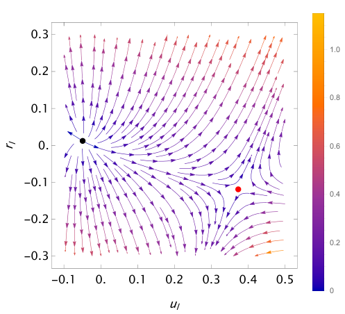
From the flow equations (B28), we see that neglecting the flow of the four-point vertex results in a runaway flow of the rescaled coupling for . This is the reason why we do not obtain a true fixed point in the level-1 truncation of Sec. III.1. On the other hand, for the rescaled six-point vertex is marginal and does not flow within our approximation, , thereby justifying the level-2 truncation used in Sec. III.2. Note that the presence of a marginal coupling may introduce additional fixed points besides the Wilson-Fisher fixed point Yabunaka17.
APPENDIX C Time-ordered correlation functions and irreducible vertices of a single spin
In this Appendix we derive the irreducible mixed five-point and six-point vertices of a single spin given in Eqs. (27) and (28). Therefore we first calculate the imaginary-time ordered spin correlation functions, and then construct the corresponding irreducible vertices using the tree expansion. In principle, all correlation functions of a single spin can be obtained by means of the generalized Wick theorem for spin operators Vaks68; Tarasevych21. In our case we only need correlation functions of the type
involving operators at vanishing frequency and one operator pair and at finite frequencies. These correlation functions can be obtained by taking derivatives of the magnetic field dependent transverse two-point function
| (C29) |
with respect to the external magnetic field using the recursion relation Rueckriegel22
| (C30) |
In particular,
| (C31) |
and
| (C32) |
Taking one more -derivative and then setting we obtain for vanishing magnetic field
| (C33) |
In this work we also need the mixed six-spin correlation function, which is for given by
| (C34) |
The corresponding irreducible vertices can be obtained from the tree expansion of connected correlation functions in terms of irreducible vertices Kopietz10. For the relevant five-point function in zero magnetic field the tree expansion is
| (C35) |
where is the static spin susceptibility of an isolated spin. A graphical representation of this relation is shown in Fig. 11.
Solving Eq. (C35) for the mixed five-point vertex, we obtain
| (C36) |
Next, we substitute our result given in Eq. (C33) for and use
| (C37) |
and
| (C38) |
Then we find that all terms cancel so that
| (C39) |
which is Eq. (27) of the main text.
Finally, consider the tree expansion of the initial value of the mixed six-point vertex
| (C40) | ||||
Solving for the mixed six-point vertex yields
| (C41) |
Substituting our result (C34) for as well as Eqs. (27) and (C38) for the lower order vertices, we obtain for the mixed six-point vertex
| (C42) |
which is Eq. (28) of the main text.
APPENDIX D Integral equation for the dynamic susceptibility
In the main text, we have used the leading term (29) of the high-temperature expansion to estimate the irreducible dynamic spin-susceptibility . In this Appendix, we explore a more sophisticated ansatz, given by
| (D43) |
where is the dissipation energy introduced in Ref. [Tarasevych21]. In the high-temperature limit the dissipation energy satisfies the approximate integral equation Tarasevych21
| (D44) |
Here, the kernel is given by
| (D45) |
where
| (D46) |
is the momentum-dependent part of the static spin self-energy to leading order in a high-temperature expansion. The flowing is then obtained by replacing the exchange coupling by its deformed counterpart, . Compared to the high-temperature approximation (29) used in the main text, this ansatz implies a non-trivial frequency dependence of that deviates from the -behavior for sufficiently small . For instance, in three dimensions one finds implying spin diffusion Tarasevych21. Another advantage of the ansatz (D43) is that it remains finite in the limit for any constant frequency. Thus, it may prove useful for the investigation of possible spin-liquid phases. However, one should keep in mind that similar to the outright high-temperature approximation (29), a high-temperature limit also underlies the validity of the integral equation (D44) Tarasevych21. Therefore, we likewise expect it to break down at the end of the flow for in the regime . A downside of this ansatz is furthermore that the Matsubara sums in the flow equations (24) and (26) can no longer be performed analytically. For the explicit numerical evaluation, we therefore used a cutoff beyond which all terms are neglected. Convergence of the sums was confirmed by comparing with results computed with twice that cutoff, .
The inverse spin susceptibility obtained with the integral equation (D44) is displayed in Fig. 12 using the interaction-switch deformation scheme to integrate the flow equations. For simplicity we focus on nearest neighbor Heisenberg magnets with spin and .
The respective critical temperatures and their relative deviations from the benchmark values are shown in Table 4.
References
- (1) H. T. Diep, Editor, Frustrated Spin Systems, (World Scientific, Singapore, 3rd Edition, 2020).
- (2) S. R. White, Density Matrix Formulation for Quantum Renormalization Groups, Phys. Rev. Lett. 69, 2863 (1992).
- (3) U. Schollwöck, The density-matrix renormalization group, Rev. Mod. Phys. 77, 259 (2005).
- (4) C. Wetterich, Exact evolution equation for the effective potential, Phys. Lett. B 301, 90 (1993).
- (5) J. Berges, N. Tetradis, and C. Wetterich, Non-perturbative renormalization flow in quantum field theory and statistical physics, Phys. Rep. 363, 223 (2002).
- (6) J. M. Pawlowski, Aspects of the functional renormalisation group, Ann. Phys. 322, 2831 (2007).
- (7) P. Kopietz, L. Bartosch, and F. Schütz, Introduction to the Functional Renormalization Group, (Springer, Berlin, 2010).
- (8) W. Metzner, M. Salmhofer, C. Honerkamp, V. Meden, and K. Schönhammer, Functional renormalization group approach to correlated fermion systems, Rev. Mod. Phys. 84, 299 (2012).
- (9) N. Dupuis, L. Canet, A. Eichhorn, W. Metzner, J. M. Pawlowski, M. Tissier, and N. Wschebor, The nonperturbative functional renormalization group and its applications, Phys. Rep. 910, 1 (2021).
- (10) C. Hille, F. B. Kugler, C. J. Eckhardt, Y.-Y. He, A. Kaush, C. Honerkamp, A. Toschi, and S. Andergassen, Quantitative functional renormalization group description of the two-dimensional Hubbard model, Phys. Rev. Research 2, 033372 (2020).
- (11) A. A. Abrikosov, Electron scattering on magnetic impurities in metals and anomalous resistivity effects, Physics 2, 5 (1965).
- (12) J. Reuther and P. Wölfle, - frustrated two-dimensional Heisenberg model: Random phase approximation and functional renormalization group, Phys. Rev. B 81, 144410 (2010).
- (13) J. Reuther and R. Thomale, Functional renormalization group for the anisotropic triangular antiferromagnet , Phys. Rev. B 83, 024402 (2011).
- (14) J. Reuther, R. Thomale, and S. Trebst, Finite-temperature phase diagram of the Heisenberg-Kitaev model, Phys. Rev. B 84, 100406(R) (2011).
- (15) F. L. Buessen and S. Trebst, Competing magnetic orders and spin liquids in two- and three-dimensional kagome systems: Pseudofermion functional renormalization group perspective, Phys. Rev. B 94, 235138 (2016).
- (16) Y. Iqbal, R. Thomale, F. P. Toldin, S. Rachel, and J. Reuther, Functional renormalization group approach for three-dimensional quantum magnetism, Phys. Rev. B 94, 140408(R) (2016).
- (17) M. L. Baez and J. Reuther, Numerical treatment of spin systems with unrestricted spin length : A functional renormalization group study, Phys. Rev. B 96, 045144 (2017).
- (18) M. Rück and J. Reuther, Effects of two-loop contributions in the pseudofermion functional renormalization group method for quantum spin systems, Phys. Rev. B 97, 144404 (2018).
- (19) J. Thoenniss, M. K. Ritter, F. B. Kugler, J. von Delft, and M. Punk, Multiloop pseudofermion functional renormalization for quantum spin systems: Application to the spin- kagome Heisenberg model, arXiv:2011.01268v1 [cond-mat.str-el] 2 Nov 2020.
- (20) D. Kiese, T. Müller, Y. Iqbal, R. Thomale, and S. Trebst, Multiloop functional renormalization group approach to quantum spin systems, Phys. Rev. Research 4, 023185 (2022).
- (21) M. K. Ritter, D. Kiese, T. Müller, F. B. Kugler, R. Thomale, S. Trebst, and J. von Delft, Benchmark Calculations of Multiloop Pseudofermion fRG, Eur. Phys. J. B 95, 102 (2022).
- (22) J. L. Martin, Generalized classical dynamics, and the ‘classical analogue’ of a Fermioscillator, Proc. R. Soc. London A 251, 536 (1959).
- (23) A. M. Tsvelik, New fermionic description of quantum spin liquid state, Phys. Rev. Lett. 69, 2142 (1992).
- (24) N. Niggemann, B. Sbierski, and J. Reuther, Frustrated quantum spins at finite temperature: Pseudo-Majorana functional renormalization group approach, Phys. Rev. B 103, 104431 (2021).
- (25) N. Niggemann, J. Reuther and B. Sbierski, Quantitative functional renormalization for three-dimensional quantum Heisenberg models, SciPost Phys. 12, 156 (2022).
- (26) J. Krieg and P. Kopietz, Exact renormalization group for quantum spin systems, Phys. Rev. B 99, 060403(R) (2019).
- (27) D. Tarasevych, J. Krieg, and P. Kopietz, A rich man’s derivation of scaling laws for the Kondo model, Phys. Rev. B 98, 235133 (2018).
- (28) R. Goll, D. Tarasevych, J. Krieg, and P. Kopietz, Spin functional renormalization group for quantum Heisenberg ferromagnets: Magnetization and magnon damping in two dimensions, Phys. Rev. B 100, 174424 (2019).
- (29) R. Goll, A. Rückriegel, and P. Kopietz, Zero-magnon sound in quantum Heisenberg ferromagnets, Phys. Rev. B 102, 224437 (2020).
- (30) D. Tarasevych and P. Kopietz, Dissipative spin dynamics in hot quantum paramagnets, Phys. Rev. B 104, 024423 (2021).
- (31) D. Tarasevych and P. Kopietz, Critical spin dynamics of Heisenberg ferromagnets revisited, Phys. Rev. B 105, 024403 (2022).
- (32) A. Rückriegel, J. Arnold, R. Goll, and P. Kopietz, Spin functional renormalization group for dimerized quantum spin systems, Phys. Rev. B 105, 224406 (2022).
- (33) A. Rançon and N. Dupuis, Nonperturbative renormalization group approach to the Bose-Hubbard model, Phys. Rev. B 83, 172501 (2011).
- (34) A. Rançon and N. Dupuis, Nonperturbative renormalization group approach to strongly correlated lattice bosons, Phys. Rev. B 84, 174513 (2011).
- (35) A. Rançon and N. Dupuis, Thermodynamics of a Bose gas near the superfluid-Mott-insulator transition, Phys. Rev. A 86, 043624 (2012).
- (36) A. Rançon, Nonperturbative renormalization group approach to quantum XY spin models, Phys. Rev. B 89, 214418 (2014).
- (37) D. F. Litim, Optimized renormalization group flows, Phys. Rev. D 64, 105007 (2001).
- (38) V. G. Vaks, A. I. Larkin, S. A. Pikin, Thermodynamics of an Ideal Ferromagnetic Substance, Zh. Eksp. Teor. Fiz. 53, 281 (1967) [ Sov. Phys. JETP 26, 188 (1968) ].
- (39) V. G. Vaks, A. I. Larkin, and S. A. Pikin, Spin waves and correlation functions in a ferromagnetic, Zh. Eksp. Teor. Fiz. 53, 1089 (1967) [ Sov. Phys. JETP 26, 647 (1968) ].
- (40) Yu. A. Izyumov and Yu. N. Skryabin, Statistical Mechanics of Magnetically Ordered Systems, (Springer, Berlin, 1988).
- (41) T. Machado and N. Dupuis, From local to critical fluctuations in lattice models: A nonperturbative renormalization-group approach, Phys. Rev. E 82, 041128 (2010).
- (42) V. Meden, W. Metzner, U. Schollwöck, and K. Schönhammer, Scaling behavior of impurities in mesoscopic Luttinger liquids, Phys. Rev. B 65, 045318 (2002).
- (43) The classical limit is obtained by rescaling , such that the Heisenberg Hamiltonian (1) remains finite in the limit. The vertex functions used throughout this work then need to be rescaled according to , , and , with initial conditions , , and .
- (44) J. Oitmaa and W. Zheng, Curie and Néel temperatures of quantum magnets, J. Phys. Condens. Matter 16, 8653 (2004).
- (45) M. Troyer, F. Alet, and S. Wessel, Histogram Methods for Quantum Systems: from reweighting to Wang-Landau Sampling, Braz. J. Phys. 34, 377 (2004).
- (46) A. W. Sandvik, Critical Temperature and the Transition from Quantum to Classical Order Parameter Fluctuations in the Three-Dimensional Heisenberg Antiferromagnet, Phys. Rev. Lett. 80, 5196 (1998).
- (47) W. Mao, P. Coleman, C. Hooley, and D. Langreth, Spin Dynamics from Majorana Fermions, Phys. Rev. Lett. 91, 207203 (2003).
- (48) A. Shnirman and Y. Makhlin, Spin-Spin Correlators in the Majorana Representation, Phys. Rev. Lett. 91, 207204 (2003).
- (49) J. Krieg, Functional renormalization group approach to classical and quantum spin systems, (PhD-Thesis, Goethe-Universität Frankfurt, 2019).
- (50) S. Yabunaka and B. Delamotte, Surprises in O(N) Models: Nonperturbative Fixed Points, Large N Limits, and Multicriticality, Phys. Rev. Lett. 119, 191602 (2017).