Doubly Robust Augmented Model Accuracy Transfer Inference with High Dimensional Features

While cohort studies remain to be critical sources for studying disease progression and treatment response, they have limitations, including the generalizability of the study findings to the real world, the limited ability to test broader hypotheses, and the cost associated with performing these studies. In recent years, due to the increasing adoption of electronic health records (EHR) and the linkage of EHR with specimen bio-repositories, integrated large datasets now exist as a new data source for deriving real-world predictive models. For example, the Massachusetts General and Brigham (MGB) Healthcare Biobank (Castro et al. 2022) and the million veteran’s project (Gaziano et al. 2016) contain a wealth of both clinical and genomic data for patients enrolled in the biobanks. These integrated datasets open opportunities for developing accurate EHR-based personalized risk prediction models, which can be easily integrated into clinical workflow to assist clinical decision-making. These models can also be contrasted and integrated with models derived from traditional cohort studies to improve generalizability.

Efficiently deriving and evaluating prediction models using EHR data remains challenging due to practical and methodological obstacles. First, gold standard labels on disease outcomes are typically not readily available in EHR and require accessibility of clinical notes and labor-intensive manual annotations. For example, at MGB, only $\sim 74\%$ of patients with at least one diagnostic code of type II diabetes (T2D) have T2D (Liao et al. 2019). On the other hand, verifying true T2D status via manual chart review is laborious and thus only available for a small number of patients at MGB. Existing methods for deriving EHR risk models typically fit prediction models to inaccurate proxies of the true outcome, such as the presence or absence of a billing code or a classification derived from a machine learning algorithm (Kurreeman et al. 2011). The misclassification error in the proxies can lead to biases in the derived prediction model and the estimated accuracy of the trained model.

Another challenge associated with ensuring the generalizability of EHR derived model arises from the heterogeneity between different EHR cohorts. It is well-known that patient populations may differ substantially across different healthcare systems, leading to significant heterogeneity in the performance of prediction models (Rasmy et al. 2018). Risk prediction models derived to optimize one EHR cohort may not perform well for another cohort. In addition, data for EHR studies are often refreshed over time as new patients enter the study, and the data of existing patients get updated. Thus, EHR data from two different time points of the same institution can have a significant shift in their distribution.

Both the scarcity of gold standard labels on disease outcomes and the covariate shift poses great challenges to generalizing knowledge about EHR-derived risk models from a labeled source population to a target population where gold standard labels are typically not available. To transfer such knowledge, much recent literature has been focused on transfer learning techniques for model estimation (Liu et al. 2020; Geva et al. 2021), such as the transportability of prediction algorithms trained from EHR data (Weng et al. 2020). On the other hand, there is a paucity of literature on transfer learning of model performance. In this paper, we propose a novel Doubly Robust Augmented Model Accuracy Transfer InferenCe (DRAMATIC) procedure to enable point and interval estimation for commonly used classification performance measures in an unlabeled target population using labeled source data. Specifically, the proposed DRAMATIC procedure develops and evaluates a prediction model for a binary response $Y$ given low dimensional predictors $\mathbf{A}$ in the target population by leveraging source data on $Y$ and high-dimensional features $\mathbf{X}=(\mathbf{A}^{\scriptscriptstyle\sf T},\mathbf{W}^{\scriptscriptstyle\sf T})^{\scriptscriptstyle\sf T}$ and only requires to be shared between the source and target data. We next detail the problem of interest and highlight our contributions in view of existing literature.

Let $Y$ denote the binary outcome of interest and $\mathbf{A}_{q\times 1}=(A_{1},\dots,A_{q})^{\scriptscriptstyle\sf T}$ denote a vector of predictors used to predict $Y$ and the first element of $\mathbf{A}$ being 1. Our goal is to develop and evaluate a risk model predicting $Y$ with $\mathbf{A}$ for a target population $\mathcal{T}$ using observed data on $n$ samples of $(Y,\mathbf{X}^{\scriptscriptstyle\sf T})^{\scriptscriptstyle\sf T}$ in a source population $\mathcal{S}$ and $N$ samples of $\mathbf{X}$ in $\mathcal{T}$, where $\mathbf{X}=(\mathbf{A}^{\scriptscriptstyle\sf T},\mathbf{W}^{\scriptscriptstyle\sf T})^{\scriptscriptstyle\sf T}$ and $\mathbf{W}_{p\times 1}=(W_{1},\dots,W_{p})^{\scriptscriptstyle\sf T}$ denotes confounding (adjustment) covariates that may relate to $Y$ and/or the distributional shift between $\mathcal{T}$ and $\mathcal{S}$. We use $S=1$ to indicate that the sample is labeled from $\mathcal{S}$ and $S=0$ for the unlabelled target data. We assume that $q$, the dimension of risk factors, is fixed but allow $p$, the dimension of the covariates $\mathbf{W}$ needed to enable transfer learning, to be high, i.e., $p\gg\min(n,N)$. In an EHR-driven genetic risk prediction study, examples of $\mathbf{A}$ include relevant genetic markers and demographic variables, while $\mathbf{W}$ may include a large number of EHR proxies of $Y$, including relevant diagnostic codes, medication prescriptions, laboratory tests, as well as mentions of clinical terms extracted from free text clinical notes via natural language processing. Hence $Y\mid\mathbf{A}$ may differ between the target and source populations, but $Y\mid\mathbf{A},\mathbf{W}$ is assumed to be the same.

To develop the risk model for $Y\mid\mathbf{A}$ in $\mathcal{T}$, we assume a working logistic regression model

which is not required to hold throughout. Here we define $\mathbb{P}_{\scriptscriptstyle\mathcal{T}}(\cdot)=\mathbb{P}(\cdot\mid S=0)$, $\mathbb{P}_{\scriptscriptstyle\mathcal{S}}(\cdot)=\mathbb{P}(\cdot\mid S=1)$, $\mathbb{E}_{\scriptscriptstyle\mathcal{T}}[\cdot]=\mathbb{E}[\cdot\mid S=0]$ and $\mathbb{E}_{\scriptscriptstyle\mathcal{S}}[\cdot]=\mathbb{E}[\cdot\mid S=1]$. Let the observed data be $\mathscr{D}=\{\mathbf{D}_{i}=(S_{i}Y_{i},\mathbf{X}_{i}^{\scriptscriptstyle\sf T},S_{i})^{\scriptscriptstyle\sf T}:i=1,2,\dots,n+N\}$ where we let $S_{i}=\mathbb{I}(1\leq i\leq n)$ without loss of generality and $\mathbb{I}(\cdot)$ is the indicator function. Assume that the samples are generated following $Y,\mathbf{X}\mid S=s\sim p_{\mathbf{X}|S=s}(\mathbf{x})\cdot p_{Y|\mathbf{X}}(y),$ where $p_{\mathbf{X}|S=s}(\cdot)$ and $p_{Y|\mathbf{X}}(\cdot)$ represent the probability mass/density function of $\mathbf{X}$ given $S$ and $Y$ given $\mathbf{X}$ respectively. Here, our underlying assumption is that distribution of covariates $\mathbf{X}$ is different across $\mathcal{S}$ and $\mathcal{T}$ while the conditional distribution of the response $Y$ given $\mathbf{X}$ is the same across the two populations. We define the density ratio function as $h_{0}(\mathbf{x})=p_{\mathbf{X}|S=0}(\mathbf{x})/p_{\mathbf{X}|S=1}(\mathbf{x})$ and the conditional mean of $Y$ on the two populations as $r_{0}(\mathbf{x})=\mathbb{E}[Y\mid\mathbf{X}=\mathbf{x}]$.

Let $\boldsymbol{\beta}_{0}$ be the outcome parameter of our interests that solves the estimating equation:

To evaluate the accuracy of the risk model $g(\mathbf{A}^{\scriptscriptstyle\sf T}\boldsymbol{\beta}_{0})$ on $\mathcal{T}$, we aim at inferring the commonly used receiver operating characteristic (ROC) curve of $Y$ against $\mathbf{A}^{\scriptscriptstyle\sf T}\boldsymbol{\beta}_{0}$. Specifically, for any given cutoff value $c$, we may classify a patient as high risk if $\mathbf{A}^{\scriptscriptstyle\sf T}\boldsymbol{\beta}_{0}\geq c$, and low risk otherwise. Then the true positive rate (TPR) and false positive rate (FPR) associated with the classification rule $\mathbb{I}(\mathbf{A}^{\scriptscriptstyle\sf T}\boldsymbol{\beta}_{0}\geq c)$ on $\mathcal{T}$ are defined as

Then the trade-off between TPR and FPR can be characterized by the ROC curve: $\mathbf{ROC}(u)=\mathbf{TPR}\{\mathbf{FPR}^{-1}(u)\}$ (Gerds et al. 2008). The overall classification performance of the risk model can be summarized based on the area under the ROC curve (AUC): $\mathbf{AUC}=\int_{0}^{1}\mathbf{ROC}(u){\rm d}u$. Our goal is to estimate the model parameter $\boldsymbol{\beta}_{0}$ and the accuracy measures $\mathbf{ROC}(\cdot)$ and $\mathbf{AUC}$ on $\mathcal{T}$ using data $\mathscr{D}$, in which $Y$ is only observed for subjects in $\mathcal{S}$ and the covariates $\mathbf{X}$ characterizing the shift between $\mathcal{S}$ and $\mathcal{T}$ are of high or ultra-high-dimensionality.

Transfer learning aims at using the information from the source population to aid the task in the target population (Torrey and Shavlik 2010), with diverse real-world applications (Liu and Stone 2006; Zhu et al. 2011; Wiens et al. 2014, e.g.). Existing machine learning methods have mainly focused on algorithms with little discussion about the theoretical guarantee, while theoretically justified transfer learning methods have largely focused on the estimation of low dimensional regression models. For example, Huang et al. 2007 proposed an importance weighting procedure based on kernel mean matching to correct for covariate shift in regression, Reddi et al. 2015 proposed a robust transfer learning strategy for removing bias while retaining small variance in parametric regression models, and Liu et al. 2020 introduced an imputation model for the response to augment importance weighting and achieved model double robustness for M-estimation.

In the era of big data, more and more application fields like EHR studies involve a potentially high-dimensional set of features in knowledge transferring to characterize the distributional shift between the source and target populations. This poses additional methodological challenges to transfer learning due to the inherent biases induced by the regularization needed to overcome the high dimensionality. Transfer learning for high-dimensional regression models has been an active area of research in recent years (Li et al. 2020; He et al. 2021; Bastani 2021; Tian and Feng 2021; Li et al. 2022, e.g.). However, limited literature exists for transfer learning of prediction performance measures in high-dimensional settings.

Existing transfer learning methods for model prediction performance can only handle the distributional shift of low-dimensional features. For example, Rotnitzky et al. 2006 developed estimators of the AUC of a single diagnostic test that adjust for selection verification. Their estimator is doubly robust in the sense of being consistent and asymptotically normal if either the outcome model or the selection-into-verification model is correct. Liu and Zhou 2010 proposed a likelihood approach to estimate the nonignorable parameter, which is not identifiable in the previous works, and proved the asymptotic normality for their AUC estimators. Semiparametric estimation of the covariate specific ROC curves with a partial missing gold standard was developed by Liu and Zhou 2011. Similarly, Long et al. 2011 aimed at estimating the AUC of a disease status given a biomarker value under a setting where the biomarker values are missing for some subjects while disease status is always confirmed and a set of auxiliary variables are fully observed.

The aforementioned methods focused on evaluating the prediction accuracy of a single predictor with low-dimensional adjustment variables for covariate shift. To the best of our knowledge, no existing work considers transfer inference for prediction accuracy of a fitted regression model in the presence of high-dimensional variables for covariates shift, which are substantially challenging due to the excessive (first-order) bias induced by high-dimensional nuisance estimators. Consequently, special debiasing techniques are needed to overcome biases induced by the high-dimensional nuisance models.

The recent works of doubly robust estimation with high-dimensional nuisance models are technically relevant to the calibrated nuisance model estimation step in our DRAMATIC method (Tan 2020; Ning et al. 2020; Dukes and Vansteelandt 2020; Liu et al. 2020). For example, Tan 2020 considered the problem of estimating average treatment effects (ATE) with high-dimensional confounding covariates under certain sparse conditions. They proposed using the calibrated estimation equations to reduce the bias incurred by the regularized error of high-dimensional regression. Their estimators are doubly robust, which remains consistent if the propensity score model or the outcome regression model is correctly specified. The calibration idea has also been adopted for ATE estimation in Ning et al. 2020 via covariate balancing and for estimating the parametric components in a semiparametric model (Dukes and Vansteelandt 2020). Liu et al. 2020 estimated the parametric component of a logistic partially linear model by deriving certain moment equations to calibrate the first-order bias of the nuisance models. Further extensions have been recently studied, for example, to alleviate the ultra-sparsity assumptions of the nuisance models at the expense of requiring both models to be correct (Bradic et al. 2019); and to solve general semiparametric estimating equations (Smucler et al. 2019; Ghosh and Tan 2020). However, none of the existing methods can be easily applied to estimate a (working) logistic model and its associated ROC curve. Estimation for the ROC curve is particularly challenging since the estimator needs to converge uniformly for all points on the curve, which necessitates controlling an infinite number of moment equations simultaneously.

Our proposed DRAMATIC method is an efficient transfer learning procedure for estimating the model coefficients and accuracy parameters that overcomes the high-dimensionality of the nuisance models while attaining robustness to model misspecifications. It involves a calibration procedure to estimate the targeted logistic regression coefficients and the TPR, FPR, ROC, and AUC parameters and attains the desirable $n^{\frac{1}{2}}$-consistency if either the high-dimensional imputation model or the high-dimensional density ratio model is correctly specified.

Our work is the first one to consider a doubly robust estimation of the ROC curve of a working classification model under the high-dimensional covariate shift regime. In this process, the excessive regularization bias incurred by the high-dimensional nuisance estimators is removed by constructing a proper set of calibrated moment equations accommodating all cutoff points on the ROC curve. In specific, we propose a “nearest quantile” strategy that ensures computation efficiency and the uniform $n^{\frac{1}{2}}$-convergence of the ROC estimators by avoiding the demand of fitting the calibrated nuisance models on the extreme left side of the ROC curve, which would result in excessive estimation errors due to the poor effective sample size. Thus, our method also exhibits novelty in view of calibrating high-dimensional nuisance models for semiparametric estimation because non-existing methods in this field can be used to calibrate the doubly robust estimators of a curve with infinite points and achieve simultaneous convergence.

Let $\widehat{\mathscr{P}}_{\scriptscriptstyle\mathcal{S}}=n^{-1}\sum_{i=1}^{n}$, $\widehat{\mathscr{P}}_{\scriptscriptstyle\mathcal{T}}=N^{-1}\sum_{i=n+1}^{N+n}$ and $\widehat{\mathscr{P}}_{{\scriptscriptstyle\mathcal{S}}{\scriptscriptstyle\cup}{\scriptscriptstyle\mathcal{T}}}={(N+n)}^{-1}\sum_{i=1}^{N+n}$ represent the empirical mean operators for the source samples, target samples and their union, respectively. Two common approaches to tackle the problem are (i) importance weighting and (ii) imputation. The former uses an estimated density ratio function $\widehat{h}(\cdot)$ to weight the source data which adjusts for covariate shift by solving the estimation equation

and the latter imputes the outcomes of the target data using an imputation function $\widehat{r}(\cdot)$ fitted by the source data, then solves the estimation equation

Although the two approaches are simple and natural, they are prone to excessive bias due to the potential model misspecification and the estimation errors of the nuisance parameters. Specifically, the importance weighting method leads to an inconsistent solution when the density ratio model $h_{0}$ is misspecified, and the imputation method is invalid when the imputation model $r_{0}$ is misspecified.

We overcome these challenges by augmenting (1) and (2) to yield a consistent estimator of $\boldsymbol{\beta}_{0}$ when either the density ratio model or the imputation model is correctly specified. To this end, we first specify the two high-dimensional nuisance models in parametric forms: $h(\mathbf{x})=\exp(\mathbf{x}^{\scriptscriptstyle\sf T}\boldsymbol{\alpha})$ and $r(\mathbf{x})=g(\mathbf{x}^{\scriptscriptstyle\sf T}\boldsymbol{\gamma})$, which are not required to hold simultaneously. Let $\widehat{\boldsymbol{\alpha}}$ and $\widehat{\boldsymbol{\gamma}}$ be some estimators for the nuisance parameters $\boldsymbol{\alpha}$ and $\boldsymbol{\gamma}$, obtained using $\ell_{1}$-regularized regression. We then introduce the doubly robust estimator for $\boldsymbol{\beta}$, denoted by $\widehat{\boldsymbol{\beta}}$, as the solution to

The double robustness of the estimation equation (3) is validated in Proposition 1.

However, unlike the low dimensional setting, due to both the potential model misspecification and the excessive estimation errors of the $\ell_{1}$-regularized nuisance estimators, simply plugging in arbitrary estimators $\widehat{\boldsymbol{\alpha}}$ and $\widehat{\boldsymbol{\beta}}$ in (3) could result in excessive first order bias and thus estimators converging slower than the desirable parametric rate even when one nuisance model is correct. Inspired by Tan 2020, we propose a bias calibration method detailed in Section 2.2 to handle this problem.

For the accuracy parameters $\mathbf{TPR}(c)$ and $\mathbf{FPR}(c)$, we propose doubly robust estimators $\widehat{\mathbf{TPR}}(c)$ and $\widehat{\mathbf{FPR}}(c)$ through augmentation similar to the construction in (3). Specifically, for any given cutoff value $c$, we construct the doubly robust estimators for the proportion of the true positives $\mathbb{P}(\mathbf{A}_{i}^{\scriptscriptstyle\sf T}\boldsymbol{\beta}_{0}\geq c,Y_{i}=1)$ and the proportion of false positives $\mathbb{P}(\mathbf{A}_{i}^{\scriptscriptstyle\sf T}\boldsymbol{\beta}_{0}\geq c,Y_{i}=0)$ as:

where the nuisance parameters $\widehat{\boldsymbol{\alpha}}_{c}$ and $\widehat{\boldsymbol{\gamma}}_{c}$ are dependent on $c$ as will be shown later. Then we take the TPR and FPR estimators as

Here, for different cut-off $c$ (and $-\infty$), we plug-in different estimators for the nuisance parameters $\boldsymbol{\alpha}_{0}$ and $\boldsymbol{\gamma}_{0}$ in the doubly robust estimators of TPR and FPR since the calibration is specific to $c$. The estimators for ROC and AUC can be constructed directly using the TPR and FPR estimators in (4) and (5), and maintain a similar doubly robust property.

We outline the DRAMATIC method in Algorithm 1 and detail the key steps in Sections 2.2 and 2.3. A multiplier bootstrap method for inference is described and discussed in Supplementary S2, whose validity is ensured by the asymptotic normality of the proposed estimators as established in Section 3.

Inspired by Tan 2020 and Dukes and Vansteelandt 2020, we construct calibrated nuisance estimators according to certain moment conditions, to correct for their regularization bias. First, we obtain preliminary estimators for $\boldsymbol{\gamma}$ in the imputation model $\mathbb{E}[Y\mid\mathbf{X}=\mathbf{x}]=g(\mathbf{x}^{\scriptscriptstyle\sf T}\boldsymbol{\gamma})$ and $\boldsymbol{\alpha}$ in density ratio $h(\mathbf{x})=\exp(\mathbf{x}^{\scriptscriptstyle\sf T}\boldsymbol{\alpha})$ as

where $G(a)=\int_{0}^{a}g(u){\rm d}u$, $\rho_{n}=(N+n)/n$, $\rho_{N}=(N+n)/N$ and $\lambda_{\gamma}$, $\lambda_{\alpha}$ are two tuning parameters. Then we solve $\mathcal{E}(\boldsymbol{\beta},\widetilde{\boldsymbol{\alpha}},\widetilde{\boldsymbol{\gamma}})=\mathbf{0}$ to obtain a preliminary estimator $\widetilde{\boldsymbol{\beta}}$. According to our discussion in Section 2.1, $\widetilde{\boldsymbol{\beta}}$ is consistent for the target $\boldsymbol{\beta}_{0}$ when either the density ratio or the imputation model is correctly specified, while it may not achieve the desirable parametric rate $n^{-1/2}$ that is crucial for asymptotic inference.

Denote the information matrix as $\bar{\boldsymbol{\Sigma}}_{\boldsymbol{\beta}}=\mathbb{E}_{\scriptscriptstyle\mathcal{S}}[\dot{g}(\mathbf{A}^{\scriptscriptstyle\sf T}\boldsymbol{\beta})\mathbf{A}\mathbf{A}^{\scriptscriptstyle\sf T}]$ and let $\widehat{\boldsymbol{\Sigma}}_{\boldsymbol{\beta}}=\widehat{\mathscr{P}}_{\scriptscriptstyle\mathcal{T}}\dot{g}(\mathbf{A}_{i}^{\scriptscriptstyle\sf T}\boldsymbol{\beta})\mathbf{A}_{i}\mathbf{A}_{i}^{\scriptscriptstyle\sf T}$ where $\dot{g}(\cdot)$ is the derivative of $g(\cdot)$. Given $\mathbf{e}_{j}\in\mathbb{R}^{q}$ the $j$th unit vector in $\mathbb{R}^{q}$ with its $j$th element being one and other elements being zero, we now focus on estimating $\mathbf{e}_{j}^{\scriptscriptstyle\sf T}\boldsymbol{\beta}_{0}$. Through asymptotic expansion, we find that the first order bias of $\sqrt{n}(\mathbf{e}_{j}^{\scriptscriptstyle\sf T}\widehat{\boldsymbol{\beta}}-\mathbf{e}_{j}^{\scriptscriptstyle\sf T}\boldsymbol{\beta}_{0})$ can be potentially controlled by the two terms¹¹ 1 We subscript the moment conditions and estimators with the symbol $\beta$ to distinguish them from those used for ROC estimation in Section 2.3.

where $\widehat{w}_{ji}(\boldsymbol{\beta})=\mathbf{e}_{j}^{\scriptscriptstyle\sf T}\widehat{\boldsymbol{\Sigma}}_{\boldsymbol{\beta}}^{-1}\mathbf{A}_{i}$ and for simplicity, we denote by $\widehat{w}_{ji}=\widehat{w}_{ji}(\widetilde{\boldsymbol{\beta}})$. The detailed derivation is presented in Supplementary S3.3. It implies that when at least one nuisance model is correctly specified, one can reduce the impact of fitting bias of the nuisance estimators plugged in (3) through controlling (7). To this end, we conduct the following regularized regressions to calibrate the nuisance estimators:

and set $\widehat{\boldsymbol{\alpha}}_{\beta_{j}}=\widetilde{\boldsymbol{\alpha}}+\widehat{\boldsymbol{\delta}}_{\beta_{j},\alpha}$, $\widehat{\boldsymbol{\gamma}}_{\beta_{j}}=\widetilde{\boldsymbol{\gamma}}+\widehat{\boldsymbol{\delta}}_{\beta_{j},\gamma}$, where

Tuning strategy of the parameters $\lambda_{\beta_{j},\alpha}$ and $\lambda_{\beta_{j},\gamma}$ is in Supplementary S1 and their rates are given in Section 3. Karush–Kuhn–Tucker (KKT) conditions of the LASSO problems (8) guarantee the $\ell_{\infty}$-terms defined in (7) to be controlled by the parameters $\lambda_{\beta_{j},\alpha}$ and $\lambda_{\beta_{j},\gamma}$, i.e. $\mathcal{M}_{\beta_{j},\alpha}(\widehat{\boldsymbol{\alpha}}_{\beta_{j}})\leq\lambda_{\beta_{j},\alpha}$ and $\mathcal{M}_{\beta_{j},\gamma}(\widehat{\boldsymbol{\gamma}}_{\beta_{j}})\leq\lambda_{\beta_{j},\gamma}$. Then we plug $\widehat{\boldsymbol{\gamma}}_{\beta_{j}}$ and $\widehat{\boldsymbol{\alpha}}_{\beta_{j}}$ in (3) to solve $\widehat{\boldsymbol{\beta}}$ from $\mathcal{E}(\boldsymbol{\beta},\widehat{\boldsymbol{\alpha}}_{\beta_{j}},\widehat{\boldsymbol{\gamma}}_{\beta_{j}})=\mathbf{0}$, and obtain $\mathbf{e}_{j}^{\scriptscriptstyle\sf T}\widehat{\boldsymbol{\beta}}$ as the estimator for $\mathbf{e}_{j}^{\scriptscriptstyle\sf T}\boldsymbol{\beta}_{0}$. To obtain the estimator for the whole $\boldsymbol{\beta}_{0}$, one can follow this procedure for $j=1,\ldots,q$ to estimate each entry of $\boldsymbol{\beta}_{0}$ separately and concatenate them together. With a little abuse of notation, we still denote the resulted vector estimator as $\widehat{\boldsymbol{\beta}}$.

Based on the estimator $\widehat{\boldsymbol{\beta}}$, we use (4) and (5) to construct the doubly robust estimators for $\mathbf{TPR}(c)$ and $\mathbf{FPR}(c)$ simultaneously for all $c\in\mathbb{R}$. Similar to Section 2.2, our goal is to derive calibrated nuisance estimators to mitigate the first order biases of $\sqrt{n}\{\widehat{\mathbf{TPR}}(c)-\mathbf{TPR}(c)\}$ and $\sqrt{n}\{\widehat{\mathbf{FPR}}(c)-\mathbf{FPR}(c)\}$. By the asymptotic analysis in Supplementary S3.4, with the initial estimators $\widetilde{\boldsymbol{\alpha}}$ and $\widetilde{\boldsymbol{\gamma}}$, we find these biases can be controlled by constructing nuisance estimators to control the error terms

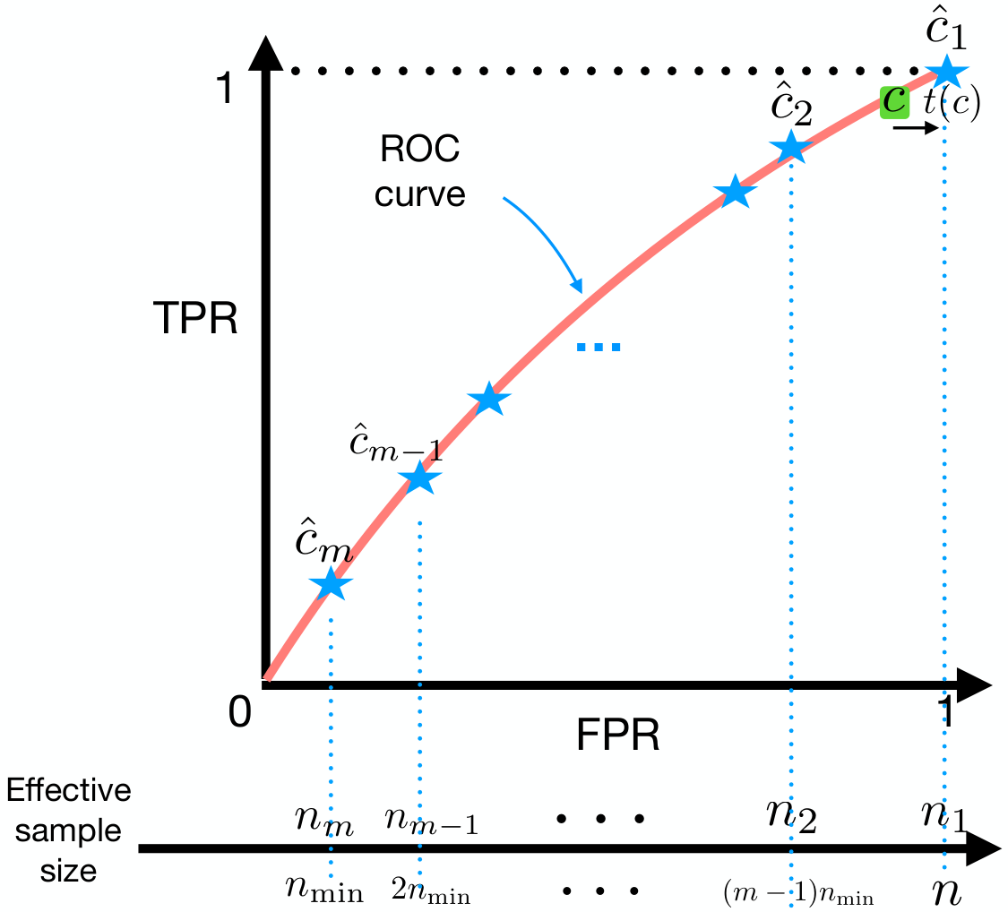
Controlling the terms in (10) is more challenging than (7) since we need to control the empirical processes $\mathcal{M}_{{\sf roc},\alpha}(\boldsymbol{\alpha};c)$ and $\mathcal{M}_{{\sf roc},\gamma}(\boldsymbol{\gamma};c)$ uniformly for $c\in\mathbb{R}$. The effective sample size for estimating TPR and FPR is also much smaller than $n$ for larger $c$, leading to additional statistical challenges. We propose a “nearest quantile” strategy that only calibrates for a sequence of cutoff values (quantiles) decided from the data. Then each point on the ROC curve will be close enough to its nearest calibrated quantile. Hence the approximation bias between them could be negligible, and one can plug in the calibrated nuisance estimators of its nearest quantile to derive the doubly robust estimator for each point.

Specifically, we split the source data into $m$ segments with equal sizes $n_{\min}=\lceil n/m\rceil$ according to the order of $\mathbf{A}_{i}^{\scriptscriptstyle\sf T}\widehat{\boldsymbol{\beta}}$, where $\lceil x\rceil$ is the smallest integer larger or equal to $x$. Without loss of generality, we assume that $\mathbf{A}_{1}^{\scriptscriptstyle\sf T}\widehat{\boldsymbol{\beta}}\geq\mathbf{A}_{2}^{\scriptscriptstyle\sf T}\widehat{\boldsymbol{\beta}}\geq\ldots\mathbf{A}_{n}^{\scriptscriptstyle\sf T}\widehat{\boldsymbol{\beta}}$. We then choose the quantiles as $\widehat{c}_{j}=\mathbf{A}_{n_{j}}^{\scriptscriptstyle\sf T}\widehat{\boldsymbol{\beta}}$ for $j\in[m]$ where $n_{1}=n,n_{2}=(m-1)n_{\min}$, $\ldots$, $n_{m}=n_{\min}$ as illustrated in Figure 1. To control the moment terms (10) corresponding to each $\widehat{c}_{j}$, we propose to solve the following calibration equations for $c\in\mathcal{C}_{\sf cal}:=\{\widehat{c}_{j}:j=1,\ldots,m\}$

and set $\widehat{\boldsymbol{\alpha}}_{{\sf roc},c}=\widetilde{\boldsymbol{\alpha}}+\widehat{\boldsymbol{\delta}}_{{\sf roc},\alpha,t(c)}$, $\widehat{\boldsymbol{\gamma}}_{{\sf roc},c}=\widetilde{\boldsymbol{\gamma}}+\widehat{\boldsymbol{\delta}}_{{\sf roc},\gamma,t(c)}$ for any $c\in\mathbb{R}$ where $t(c)=\mathop{\mbox{argmin}}_{c^{\prime}\in\mathcal{C}_{\sf cal}}|c^{\prime}-c|$. Here $\lambda_{{\sf roc},\alpha,\widehat{c}_{j}}$ and $\lambda_{{\sf roc},\gamma,\widehat{c}_{j}}$ are two series of $\ell_{1}$-penalty parameters to be tuned using the procedure described in Supplementary S1. We then construct the doubly robust estimators for $\mathbf{TPR}(\cdot)$ and $\mathbf{FPR}(\cdot)$ based on the calibrated nuisance estimators and plug the estimators $\widehat{\boldsymbol{\alpha}}_{{\sf roc},t(c)}$ and $\widehat{\boldsymbol{\gamma}}_{{\sf roc},t(c)}$ into (5) to obtain

Finally, one can evaluate $\widehat{\mathbf{ROC}}(u)=\widehat{\mathbf{TPR}}\{{\widehat{\mathbf{FPR}}}^{-1}(u)\}$, and $\widehat{\mathbf{AUC}}=\int_{0}^{1}\widehat{\mathbf{ROC}}(u){\rm d}u$, to estimate the ROC function and AUC. An illustration of this “nearest quantile” strategy is presented in Figure 1.

References

- Bang and Robins (2005) Bang, H. and J. M. Robins (2005). Doubly robust estimation in missing data and causal inference models. Biometrics 61(4), 962–973.
- Bastani (2021) Bastani, H. (2021). Predicting with proxies: Transfer learning in high dimension. Management Science 67(5), 2964–2984.
- Bradic et al. (2019) Bradic, J., S. Wager, and Y. Zhu (2019). Sparsity double robust inference of average treatment effects. arXiv preprint arXiv:1905.00744.
- Bühlmann and Van De Geer (2011) Bühlmann, P. and S. Van De Geer (2011). Statistics for high-dimensional data: methods, theory and applications. Springer Science & Business Media.
- Castro et al. (2022) Castro, V. M., V. Gainer, N. Wattanasin, B. Benoit, A. Cagan, B. Ghosh, S. Goryachev, R. Metta, H. Park, D. Wang, et al. (2022). The mass general brigham biobank portal: an i2b2-based data repository linking disparate and high-dimensional patient data to support multimodal analytics. Journal of the American Medical Informatics Association 29(4), 643–651.
- Chakrabortty and Cai (2018) Chakrabortty, A. and T. Cai (2018). Efficient and adaptive linear regression in semi-supervised settings. The Annals of Statistics 46(4), 1541–1572.
- Dukes and Vansteelandt (2020) Dukes, O. and S. Vansteelandt (2020). Inference on treatment effect parameters in potentially misspecified high-dimensional models. Biometrika.
- Gaziano et al. (2016) Gaziano, J. M., J. Concato, M. Brophy, L. Fiore, S. Pyarajan, J. Breeling, S. Whitbourne, J. Deen, C. Shannon, D. Humphries, et al. (2016). Million veteran program: A mega-biobank to study genetic influences on health and disease. Journal of clinical epidemiology 70, 214–223.
- Gerds et al. (2008) Gerds, T. A., T. Cai, and M. Schumacher (2008). The performance of risk prediction models. Biometrical Journal: Journal of Mathematical Methods in Biosciences 50(4), 457–479.
- Geva et al. (2021) Geva, A., M. Liu, V. A. Panickan, P. Avillach, T. Cai, and K. D. Mandl (2021). A high-throughput phenotyping algorithm is portable from adult to pediatric populations. Journal of the American Medical Informatics Association.
- Ghosh and Tan (2020) Ghosh, S. and Z. Tan (2020). Doubly robust semiparametric inference using regularized calibrated estimation with high-dimensional data. arXiv preprint arXiv:2009.12033.
- Gronsbell et al. (2022) Gronsbell, J., M. Liu, L. Tian, and T. Cai (2022). Efficient estimation and evaluation of prediction rules in semi-supervised settings under stratified sampling. JOURNAL OF THE ROYAL STATISTICAL SOCIETY SERIES B-STATISTICAL METHODOLOGY.
- Gronsbell and Cai (2018) Gronsbell, J. L. and T. Cai (2018). Semi-supervised approaches to efficient evaluation of model prediction performance. Journal of the Royal Statistical Society: Series B (Statistical Methodology) 80(3), 579–594.
- Hahn (1998) Hahn, J. (1998). On the role of the propensity score in efficient semiparametric estimation of average treatment effects. Econometrica, 315–331.
- He et al. (2021) He, Y., C. M. Lakhani, D. Rasooly, A. K. Manrai, I. Tzoulaki, and C. J. Patel (2021). Comparisons of polyexposure, polygenic, and clinical risk scores in risk prediction of type 2 diabetes. Diabetes Care 44(4), 935–943.
- He et al. (2021) He, Y., Q. Li, Q. Hu, and L. Liu (2021). Transfer learning in high-dimensional semi-parametric graphical models with application to brain connectivity analysis. arXiv preprint arXiv:2112.13356.
- Hong et al. (2021) Hong, C., E. Rush, M. Liu, D. Zhou, J. Sun, A. Sonabend, V. M. Castro, P. Schubert, V. A. Panickan, T. Cai, et al. (2021). Clinical knowledge extraction via sparse embedding regression (keser) with multi-center large scale electronic health record data. NPJ digital medicine 4(1), 1–11.
- Huang et al. (2007) Huang, J., A. Gretton, K. Borgwardt, B. Schölkopf, and A. J. Smola (2007). Correcting sample selection bias by unlabeled data. In Advances in neural information processing systems, pp. 601–608.
- Kawakita and Kanamori (2013) Kawakita, M. and T. Kanamori (2013). Semi-supervised learning with density-ratio estimation. Machine learning 91(2), 189–209.
- Kurreeman et al. (2011) Kurreeman, F., K. Liao, L. Chibnik, B. Hickey, E. Stahl, V. Gainer, G. Li, L. Bry, S. Mahan, K. Ardlie, et al. (2011). Genetic basis of autoantibody positive and negative rheumatoid arthritis risk in a multi-ethnic cohort derived from electronic health records. The American Journal of Human Genetics 88(1), 57–69.
- Li et al. (2020) Li, S., T. T. Cai, and H. Li (2020). Transfer learning for high-dimensional linear regression: Prediction, estimation, and minimax optimality. arXiv preprint arXiv:2006.10593.
- Li et al. (2022) Li, S., T. T. Cai, and H. Li (2022). Transfer learning in large-scale gaussian graphical models with false discovery rate control. Journal of the American Statistical Association, 1–13.
- Liao et al. (2019) Liao, K. P., J. Sun, T. A. Cai, N. Link, C. Hong, J. Huang, J. E. Huffman, J. Gronsbell, Y. Zhang, Y.-L. Ho, et al. (2019). High-throughput multimodal automated phenotyping (map) with application to phewas. Journal of the American Medical Informatics Association 26(11), 1255–1262.
- Liu and Zhou (2010) Liu, D. and X.-H. Zhou (2010). A model for adjusting for nonignorable verification bias in estimation of the roc curve and its area with likelihood-based approach. Biometrics 66(4), 1119–1128.
- Liu and Zhou (2011) Liu, D. and X.-H. Zhou (2011). Semiparametric estimation of the covariate-specific roc curve in presence of ignorable verification bias. Biometrics 67(3), 906–916.
- Liu et al. (2020) Liu, M., Y. Zhang, K. P. Liao, and T. Cai (2020). Augmented transfer regression learning with semi-non-parametric nuisance models. arXiv.
- Liu et al. (2020) Liu, M., Y. Zhang, and D. Zhou (2020). Double/debiased machine learning for logistic partially linear model. arXiv preprint arXiv:2009.14461.
- Liu and Stone (2006) Liu, Y. and P. Stone (2006). Value-function-based transfer for reinforcement learning using structure mapping. In AAAI, pp. 415–420.
- Long et al. (2011) Long, Q., X. Zhang, and B. A. Johnson (2011). Robust estimation of area under roc curve using auxiliary variables in the presence of missing biomarker values. Biometrics 67(2), 559–567.
- Mahajan et al. (2018) Mahajan, A., D. Taliun, M. Thurner, N. R. Robertson, J. M. Torres, N. W. Rayner, A. J. Payne, V. Steinthorsdottir, R. A. Scott, N. Grarup, et al. (2018). Fine-mapping type 2 diabetes loci to single-variant resolution using high-density imputation and islet-specific epigenome maps. Nature genetics 50(11), 1505–1513.
- Negahban et al. (2012) Negahban, S. N., P. Ravikumar, M. J. Wainwright, B. Yu, et al. (2012). A unified framework for high-dimensional analysis of M-estimators with decomposable regularizers. Statistical Science 27(4), 538–557.
- Ning et al. (2020) Ning, Y., P. Sida, and K. Imai (2020). Robust estimation of causal effects via a high-dimensional covariate balancing propensity score. Biometrika 107(3), 533–554.
- Rasmy et al. (2018) Rasmy, L., Y. Wu, N. Wang, X. Geng, W. J. Zheng, F. Wang, H. Wu, H. Xu, and D. Zhi (2018). A study of generalizability of recurrent neural network-based predictive models for heart failure onset risk using a large and heterogeneous ehr data set. Journal of biomedical informatics 84, 11–16.
- Reddi et al. (2015) Reddi, S. J., B. Poczos, and A. Smola (2015). Doubly robust covariate shift correction. In Twenty-Ninth AAAI Conference on Artificial Intelligence.
- Rotnitzky et al. (2006) Rotnitzky, A., D. Faraggi, and E. Schisterman (2006). Doubly robust estimation of the area under the receiver-operating characteristic curve in the presence of verification bias. Journal of the American Statistical Association 101(475), 1276–1288.
- Shu and Tan (2018) Shu, H. and Z. Tan (2018). Improved estimation of average treatment effects on the treated: Local efficiency, double robustness, and beyond. arXiv preprint arXiv:1808.01408.
- Smucler et al. (2019) Smucler, E., A. Rotnitzky, and J. M. Robins (2019). A unifying approach for doubly-robust -regularized estimation of causal contrasts. arXiv preprint arXiv:1904.03737.
- Tan (2020) Tan, Z. (2020). Model-assisted inference for treatment effects using regularized calibrated estimation with high-dimensional data. Annals of Statistics 48(2), 811–837.
- Tian and Feng (2021) Tian, Y. and Y. Feng (2021). Transfer learning under high-dimensional generalized linear models. arXiv preprint arXiv:2105.14328.
- Torrey and Shavlik (2010) Torrey, L. and J. Shavlik (2010). Transfer learning. In Handbook of research on machine learning applications and trends: algorithms, methods, and techniques, pp. 242–264. IGI global.
- Weng et al. (2020) Weng, C., N. H. Shah, and G. Hripcsak (2020). Deep phenotyping: embracing complexity and temporality—towards scalability, portability, and interoperability. Journal of biomedical informatics 105, 103433.
- Wiens et al. (2014) Wiens, J., J. Guttag, and E. Horvitz (2014). A study in transfer learning: leveraging data from multiple hospitals to enhance hospital-specific predictions. Journal of the American Medical Informatics Association 21(4), 699–706.
- Zhu et al. (2011) Zhu, Y., Y. Chen, Z. Lu, S. J. Pan, G.-R. Xue, Y. Yu, and Q. Yang (2011). Heterogeneous transfer learning for image classification. In Twenty-fifth aaai conference on artificial intelligence.