Relativistic quantum thermometry through a moving sensor
Abstract
Using a two-level moving probe, we address the temperature estimation of a static thermal bath modeled by a massless scalar field prepared in a thermal state. Different couplings of the probe to the field are discussed under various scenarios. We find that the thermometry is completely unaffected by the Lamb shift of the energy levels. We take into account the roles of probe velocity, its initial preparation, and environmental control parameters for achieving optimal temperature estimation. We show that a practical technique can be utilized to implement such a quantum thermometry. Finally, exploiting the thermal sensor moving at high velocity to probe temperature within a multiparameter-estimation strategy, we demonstrate perfect supremacy of the joint estimation over the individual one.
I Introduction
Temperature estimation is an important task on all scales, ranging from atomic systems near absolute zero to astronomical bodies of high temperatures. Particularly, applications of thermometry in microscale and nanoscale devices are becoming in great demand as technology advances Yue and Wang 2012; Giazotto et al. 2006; Carlos and Palacio 2015; Mehboudi et al. 2019a. Examples include precise temperature estimation of ultracold gases Sabín et al. 2014; Mehboudi et al. 2019b; Bouton et al. 2020, electrons in superconductors Gasparinetti et al. 2015; Halbertal et al. 2016, and the application of atomic-size devices such as quantum dots or color centers in diamond, when probes are used in various systems Kucsko et al. 2013; Neumann et al. 2013; Haupt et al. 2014; Hovhannisyan et al. 2021. The classical approach to thermometry is that the state of thermometer, brought into thermal contact with a sample, is monitored for some time, conveying the information about the sample temperature Jørgensen et al. 2020.
In the quantum realm, thermodynamical quantities are usually challenging to define, manipulate and measure Binder et al. 2018, to the point that they may lead to reformulation of the thermodynamics laws Levy et al. 2012; Kolář et al. 2012; Brandao et al. 2015; Uzdin and Rahav 2018; Mehboudi et al. 2019a. Recent advancements in quantum metrology Helstrom 1969; Paris 2009; Giovannetti et al. 2006; Giovannetti et al. 2011; Degen et al. 2017; Pirandola et al. 2018; Pezze et al. 2018; Huang et al. 2019; Liu et al. 2022; Rangani Jahromi and Franco 2021; Rangani Jahromi 2018 have led to extension of thermodynamics boundaries into novel territories, in which tiny objects are cooled to ultra-low temperatures Giazotto et al. 2006; Bloch et al. 2008, and resulted in the development of a fast-growing field of research, i.e., quantum thermometry Goold et al. 2016; Stace 2010; Seah et al. 2019; Montenegro et al. 2020; Zhang and Wu 2021; Mok et al. 2021; Mancino et al. 2020; Rubio et al. 2021; Paris 2015; Pasquale and Stace 2018; Correa et al. 2017; Planella et al. 2022; Hovhannisyan et al. 2021; Alves and Landi 2022; Jørgensen et al. 2020; Gebbia et al. 2020; Luiz et al. 2022; O’Connor et al. 2021; Kenfack et al. 2021; Farajollahi et al. 2018; Jahromi 2020. The basic idea is to estimate the temperature of a thermal environment by letting it interact with a quantum system, say a qubit or a pair of entangled qubits, called a quantum probe, which are then subsequently measured to extract the information. Applying quantum probes to estimate parameters of interest has the advantage that it does not perturb too much the system under investigation. Provided that the probe reaches a non-equilibrium steady state, or thermal equilibrium with the sample, the optimal measurement, minimizing the uncertainty of the thermometry through saturating the Cramér-Rao inequality Paris 2009 may be achievable Correa et al. 2015; Correa et al. 2017; Mehboudi et al. 2019b; Hofer et al. 2017; Guarnieri et al. 2019; Jørgensen et al. 2020. In the non-equilibrium dynamics where the temperature is extracted from the state of the probe before its thermalization Montenegro et al. 2020; Brunelli et al. 2012; De Pasquale et al. 2017; Feyles et al. 2019; Gebbia et al. 2020; Seah et al. 2019; Mancino et al. 2020, the optimal thermometry, generally depends on the unknown temperature of the system, making its achievement challenging in practice Mok et al. 2021.
In near-equilibrium thermometry, it is known that the energy measurement is the optimal choice Correa et al. 2015; Marzolino and Braun 2013; Hovhannisyan et al. 2021, as happens in classical physics. Nonetheless, this approach may be very demanding, because it requires access to the total system, measurement of its energy and full knowledge of the spectrum. However, when a small quantum probe interacts with the system without causing much disturbance and then it is measured, those limitations are not encountered Montenegro et al. 2020; Mok et al. 2021. These considerations motivate more investigation of quantum metrology in the context of near-equilibrium thermometry, especially for relativistic scenarios in which the observed temperature by the moving system is a challenging discussion Papadatos and Anastopoulos 2020; Cai 2021.
Quantum field theory indicates that different noninertial observers do not agrees on the number of particles in a given field state. In fact, a quantum (scalar) field in the Minkowski-Unruh vacuum from an inertial perspective is observed as a thermal bath by a Rindler observer moving with uniform acceleration; this phenomenon is known as Unruh effect Crispino et al. 2008; Schlicht 2004. Quantum estimation of the Unruh temperature by various accelerated probes have been investigated in some references Aspachs et al. 2010; Tian et al. 2015; Wang et al. 2014; Feng and Zhang 2022; Patterson and Mann 2022. Moreover, in the absence of Unruh effect, the temperature estimation through a static atom immersed in a thermal bath with a boundary in a massless scalar field has been analyzed in Zhao et al. 2020. In addition, the performance of estimating the parameters encoded into the initial state of a two-level probe, moving with a constant velocity, as the detector coupled to a massless scalar field, has been also studied Liu et al. 2021. It has been shown that the estimation is completely unaffected by the velocity, however, it becomes more inaccurate over time because of the decoherence caused by the interaction between the atom and the field. Hence, it would be interesting to investigate how quantum thermometry is affected in this scenario.
In this paper, we consider an Unruh-DeWitt (UDW) detector Costa and Matsas 1995 moving with constant velocity and interacting with a thermal scalar field. Because of this interaction, the UDW detector Unruh 1976; Hu et al. 2012 is an open quantum system Moustos 2018; Zhao et al. 2020; Papadatos and Anastopoulos 2020; Liu et al. 2021; Ng et al. 2018; Jafarzadeh et al. 2018; Rangani Jahromi 2019 encoding the information on the temperature of the field, and hence playing the role of a quantum thermometer. Employing a moving probe for quantum estimation is a powerful technique, especially when the metrological setup used to analyze and extract information from the probe is located elsewhere. Here, after computing quantum Fisher information, a reliability measure of the moving probe as a temperature sensor, we investigate how the initial parameters, as well as the ambient ones, can be controlled to improve the thermometry. In particular, we find that control over the probe velocity plays a key role to achieve optimal accuracy. We also elaborate on a physical proposition for the experimental implementation of the quantum thermometry. Finally, we discuss how the thermometer can be used for the simultaneous estimation of parameters and illustrate the perfect supremacy of quantum thermometry in a multiparameter-estimation scenario.
The paper is structured as follows: In Sec. II, a brief review of the theory of quantum metrology is presented. Then, we introduce the model in Sec. III. The process of quantum thermometry is completely investigated in Sec. IV. Finally, Sec. V is devoted to summarizing and discussing the most important results. Throughout this paper, we apply units with . Moreover, a simple set of scaled units is introduced Jahromi and Amniat-Talab 2015 in Table I.
| Physical quantity | Scaled unit | SI unit |
|---|---|---|
| Temperature: | 1 | |
| Angular Frequency: | 1 | |
| Time: | 1 | |
| Coupling constant: | 1 |
II Quantum Fisher information
Quantum Fisher information Braunstein and Caves 1994, determining the fundamental limit to the accuracy of estimating an unknown parameter, plays the most key role in quantum metrology. First we concisely review the principles of classical estimation theory and introduce the tools which it provides to calculate the bounds to accuracy of any quantum metrology process. In an estimation problem we aim at extracting the value of a parameter through measuring a related quantity . For solving this problem, one should obtain an estimator , generating an estimate for the parameter , based on the achieved measurement outcomes . In the classical theory, the variance of any unbiased estimator, in which denotes the mean with respect to the identically distributed random variables , fulfills the Cramer-Rao inequality where indicates the number of independent measurements. This inequality gives a lower bound on the variance in terms of the the Fisher information (FI)
| (1) |
in which signifies the conditional probability of obtaining the value as the unknown parameter has the value . When the eigenvalue spectrum of observable is continuous, the summation in Eq. (1) must be replaced by an integral.
In the quantum regime in which indicates the state of the quantum system and represents the probability operator-valued measure (POVM) characterizing the measurement. In brief summary, it is feasible to indirectly achieve the value of the physical parameter, intending to estimate it, through measuring an observable and then making statistical analysis on the measurement outcomes. An estimator is called efficient when it at least asymptotically saturates the Cramer-Rao bound.
Obviously, various observables result in various probability distributions, giving rise to miscellaneous FIs and therefore to different precision for estimation of . The ultimate bound to the precision, determined by the quantum Fisher information (QFI), is attained by maximizing the FI over the set of the observables. The QFI of an unknown parameter encoded into the quantum state is given by Helstrom 1969; Braunstein and Caves 1994; Paris 2009
| (2) |
where indicates the corresponding symmetric logarithmic derivative (SLD) given by in which . As is well-known, the set of projectors over the eigenvectors of the SLD gives an optimal POVM.
An explicit expression of the QFI can be obtained for single-qubit systems. It is known that any qubit state can be written in the Bloch sphere representation as , in which denotes the Bloch vector and represents the Pauli matrice, leading to the following compact formula for the QFI of the single-qubit state Zhong et al. 2013
| (3) |
where is used for a mixed (pure) state.
III Model
We consider a composite quantum system consisting of a microscopic two-level probe S, for example, an atom or a molecule, and a quantum scalar field Papadatos and Anastopoulos 2020. The system is characterized by a Hilbert space , in which () denotes the Hilbert space of the probe (field). The Hamiltonian is given by
| (4) |
where represents the Hamiltonian generating time translations with respect to proper time parameter of . The Hamiltonian , describing a free massless scalar field, is given by in which denotes the conjugate momentum of the field . The general form of the interaction terms is where represents a coupling constant, denotes a self-adjoint operator on , and designates a local composite operator for the scalar field. Moreover, the trajectory , in which represents the detector path, is given by
| (5) |
where represents the rapidity of the trajectory, associated with velocity , and denotes a coupling constant.
We assume a seperable initial state where represents a Gibbs state at temperature , . We focus on two different coupling regimes, i.e., (i) and (ii) representing, respectively, the Unruh-DeWitt (UDW) and time-derivative (TD) couplings.
Starting from the Hamiltonian (4) with the separable initial states and defining the transition operators
| (6) |
one can extract the the reduced dynamics of the probe from the following second-order master equation
| (7) |
where denotes the set of all energy differences. Moreover, in which represents the Lamb shift of the energy levels, and
| (8) |
For the UDW coupling with positive , the expressions for and are given by
| (9) |
| (10) |
where in which , denotes the expected numbers of particles of momentum k. Moreover,
| (11) |
where
| (12) |
indicates the contribution for the Lamb-Shift. In (12) and signify, respectively, the cutoff and the Euler-Macheronni constant.
The corresponding expressions for , , and in the TD-coupling regime are
| (13) |
| (14) |
and
| (15) |
where
| (16) |
We assume the Hamiltonian of the two-level atom characterized by frequency is given by and the coupling operator is expressed as , resulting in two transition operators and . Solving the corresponding master equation for the initial pure state
| (17) |
one finds that the evolved density matrix of the probe is given by
| (18) |
where . Moreover, = denotes the decay coefficient for the atom in the vacuum, represents the Lamb-shifted excitation frequency.
IV Quantum thermometry
We apply the two-level atom for estimating the initial temperature of the quantum field. The information on the temperature is stored into the evolved state of the total system, and hence is used by the two-level atom to probe it. To this aim, we compute the QFI corresponding to the temperature and analyze its behavior. In particular, we focus on the QFI optimization with respect to initial as well as environmental parameters to achieve optimal thermometry. Using Eqs. (18) and (3) with , we obtain the following analytical expression for the QFI:
| (19) |
where and .
We focus on two different couplings of the moving system to the thermal bath, and investigate quantum thermometry in two important ranges, i.e., low as well as normal temperatures. The first important result is that the QFI is independent of , and hence in both regimes the thermometry is unaffected by the Lamb-shifted excitation frequency. Moreover, we see that the QFI is independent of , and thereby no control over the initial phase is required to achieve the best estimation of the temperature.
IV.1 Low-temperature and UDW-coupling regime


Studying the QFI behavior for and UDW coupling, we find that when the atom is initially prepared in the ground state , the best estimation can be achieved (see Fig. 1). Therefore, we set throughout this paper. Moreover, as demonstrated in Fig. (1), when the coupling constant , quantifying the strength of interaction between the probe and the field, increases, the QFI rises, enhancing the accuracy of the quantum estimation.
Figure 2 illustrates how the rapidity of the trajectory affects the thermometry accuracy at different low temperatures. It shows that the QFI first improves with an increase in and then decreases. Although strengthening the coupling constant, one can enhance the estimation, we see from Fig. 2 that, in the weak-coupling regime, an increase in , cannot shift the optimal value of at which the best estimation occurs. In addition, Fig. 2 shows that an increase in reduces the accuracy of the optimal estimation and shifts the optimal value of , at which the best estimation occurs, to higher velocities.
As clear in Figs. 1 and 2, the QFI first grows with an increase in the temperature and then falls. Figure 3 illustrates how the variation of the probe velocity affects this fall. It shows that by increasing , the optimal value of the QFI versus T is achieved in lower temperatures. However, it may cause the optimal value to decrease, thus reducing the precision of the estimation.
Monitoring the dynamics of the quantum thermometry through studying the QFI shows when time goes on, the QFI improves, as expected, however, then it decays (see Fig. 3 ). Control of this reduction, studied in Figs. 3 and 4, is of great interest. Figure 3 displays that an increase in removes the QFI dropping with time and results in the QFI trapping exhibiting asymptotic behavior with some definite value. However, after the appearance of the QFI trapping, a further increase in suppresses the QFI, although it causes the QFI trapping to appear sooner. Therefore, to investigate the QFI dynamics in the low-temperature scenario, the low-frequency regime, where the QFI exhibits an optimum point, and the high-frequency one, in which the QFI trapping occurs, should be studied separately.
Figure 4 illustrates a positive and interesting effect of a rise in the coupling constant. It demonstrates that when it is raised in the low-frequency regime, the optimal value of the QFI, signifying the best instance for quantum thermometry, is achieved sooner. Nevertheless, this strategy brings the QFI loss forward, and hence the period at which the thermometry can be implemented efficiently is shortened.
The QFI variations versus time for different values of and in the high-frequency regime are displayed in Figs. 4 and 4, respectively. Clearly, when the interaction between the probe and field is strengthened by an increase in , the estimation enhances and it causes the QFI trapping to appear more quickly. Moreover, as clear from Fig. 4, speeding up the probe, applied for the thermometry, retards the QFI.
IV.2 Low-temperature and TD-coupling regime
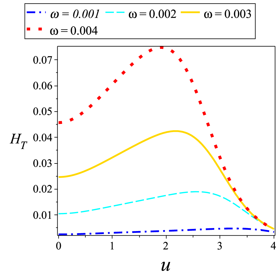
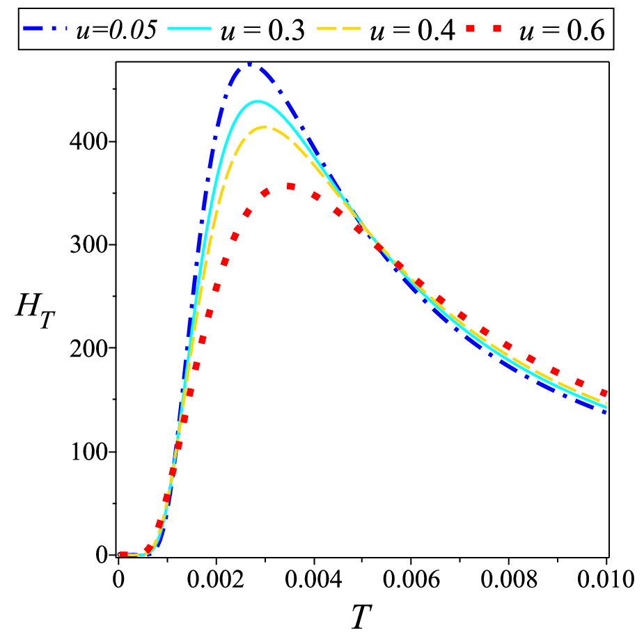

In this section, we focus on the quantum thermometry when the temperature is sufficiently low in the TD-coupling regime. Most of the results presented for the UDW coupling also hold here, and hence we only present the deviations.
In the TD-coupling regime, although the best estimation is achieved for , we see that at high velocities, the QFI does not vary considerably with . Therefore, when the probe moves at high speeds, it is not necessary to initially prepare it in the ground state to achieve the best estimation.
Moreover, in the UDW-coupling we saw that enhancement of the thermometry was limited to certain circumstances. For example, strengthening the interaction between the probe and the field does not necessarily lead to the estimation improvement in the low-frequency and UDW -coupling regime. However, in the TD coupling, we find that an increase in always improves the accuracy of the temperature estimation.
Figure 5 illustrates that an increase in raises the accuracy of the optimal thermometry and shifts the optimal value of , at which the best estimation is achieved, to lower velocities.
Another difference between the UDW- and TD-coupling regimes is demonstrated in Fig. 5 exhibiting how the variation of the probe velocity influences the QFI decay occurring with an increase in the temperature. We see that speeding up the probe negatively affects low-temperature thermometry, because it shifts the optimal value of the QFI to higher temperatures. Similar to UDW coupling, we find that raising suppresses the optimal value of the QFI versus , reflecting that the thermometry becomes more inaccurate. Moreover, investigating the QFI dynamics at high frequencies in which the QFI trapping occurs reveals that a decrease in retards the QFI trapping (see Fig. 5).
IV.3 Normal-temperature and UDW-coupling regime


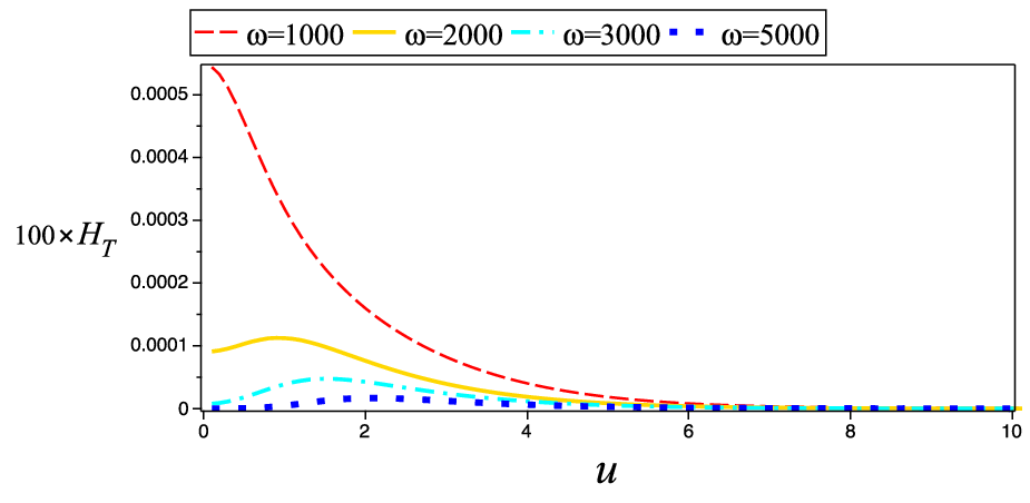
Now we investigate the normal-temperature thermometry in the range and present the most important results. First, we find that, at high velocities, the best estimation is achieved for (see Fig. 6). Therefore, probes moving at high speeds should be initially prepared in the ground state to implement the optimal thermometry. Moreover, similar to the low-temperature regime, to study the QFI dynamics, we should consider two different scenarios: 1) the low-frequency regime in which the QFI first increases with time and then decreases; 2) the high-frequency regime where the QFI trapping occurs.
For high frequencies, we find that the QFI dynamics is similar to one observed in the low-temperature regime. Therefore, 1) an increase in and causes the QFI trapping to appear sooner; 2) a rise in improves the QFI; 3) an increase in u retards the QFI trapping.
For low frequencies in which the QFI is suppressed with time, an increase (a decrease) in retards the QFI loss during the evolution and hence enhances the estimation of the parameter at periods in which the QFI tends to zero. However, a decrease (an increase) in leads to the occurrence of the optimal estimation at an earlier time. In particular, it does not vary the optimal value of the QFI. These results are exhibited in Figs. 7 and 7.
IV.4 Normal-temperature and TD-coupling regime

Focusing on TD-coupling and normal-temperature regime, we see that the results extracted from Figs. 6 and 7 for UDW coupling, also hold here. However, investigating the behavior of the QFI versus , we find that in the low-frequency regime, an increase in results in the occurrence of the optimal estimation in lower velocities. In particular, as demonstrated in Fig. 9, it does not considerably vary the optimal value of QFI.
IV.5 Practicable measurement for optimal thermometry
A major question that may arise is how we can physically implement the optimal thermometry, i.e., a practicable measurement for which the corresponding Fisher information equals the QFI. Noting that the optimal POVM can be made by the eigenvectors of the SLD, we focus on computing them and checking whether these eigenstates overlap with those of some physical observable of the system. Interestingly, following this prescription, we find that when the probe is initially prepared in the ground state (), the optimal POVM can be constructed by the eigenvectors of . In other words, the measurement of on the probe leads to the optimal quantum thermometry, saturating the quantum upper bound. This result is absolutely important because not only the optimal POVM but also the maximized QFI is achieved when the atom is initially prepared in the ground state.
IV.6 Quantum thermometry in a multiparameter-estimation strategy
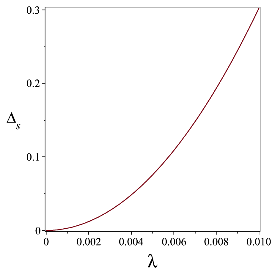

Because the QFI is usually optimized for , investigating the simultaneous estimation of and is of great importance for the realization of the optimal thermometry. In particular, we should examine the supremacy of simultaneous estimation in comparison with the individual one. First, some background on the multiparameter estimation theory is presented.
A quantum system applied in a quantum estimation problem can be characterized by a quantum state a function of unknown parameters . A multi-parameter quantum estimation strategy is a hunt for the best precision accessible in the simultaneous estimation of Szczykulska et al. 2016. The quantum Cramer-Rao bound (QCRB), providing a lower bound for the mean square errors of the parameters , can be formally expressed as Liu et al. 2019
| (20) |
where is the number of experimental runs and denotes the covariance matrix of any locally unbiased estimators of the parameters . Moreover, represents the quantum Fisher information matrix whose components are given by
| (21) |
where denotes the symmetric logarithmic derivatives (SLD), corresponding to parameter , written as
| (22) |
in which . It should be noted that although the bound in Eq. (20) is not always tight, the multiparameter QCRB can be saturated provided that the following compatibility condition is satisfied Ragy et al. 2016; Napoli et al. 2019
| (23) |
Defining ratio Yousefjani et al. 2017:
| (24) |
where the minimal total variances in the individual and simultaneous estimations are represented, respectively, by and , one can collate the performance of the simultaneous estimation in comparison with that of the individual one. Comparing independent and simultaneous schemes, we find that in the simultaneous-estimation strategy fewer resources are required by a factor of the number of parameters to be estimated, and therefore considering in the definition of is necessary to account for this reduction in resources. The efficiency of simultaneous estimation rather than the independent one can be signified by 1. Assuming a single run of the experimental measurement, we put throughout the paper.
In our model, computing the expectation value of commutator on the probe state, we find that it vanishes, i.e., , indicating that the multiparameter QCRB can be saturated. In other words Vidrighin et al. 2014, there is a single measurement that is jointly optimal to extract information on and from the output state, guaranteeing the asymptotic saturability of the QCRB.
In the UDW-coupling regime, more results of interest can be obtained. The most important one is that at a high-velocity regime, is roughly maximized, i.e., , indicating complete superiority of the simultaneous strategy over the individual one through fast-moving probes. In general, where denotes the number of parameters to be estimated. Moreover, as shown in Fig. 10, at the high-velocity regime, grows with an increase in , and hence better accuracy occurs for weaker couplings. In addition, Fig. 10 demonstrates that total variance is always minimized for , indicating the importance of initially preparing the probe in the ground state to achieve the best simultaneous estimation.
V Conclusions
We investigated relativistic quantum thermometry through a moving probe playing the role of a thermal sensor. It is employed to estimate the temperature of a heat bath modeled by a massless scalar field initially prepared in a thermal state. The effects of the Lamb shift, the initial preparation of the sensor as well as its velocity, and ambient control parameters on the thermometer sensitivity have been analyzed in detail to enhance the quantum estimation. Moreover, quantum thermometry in a multiparameter-estimation scenario has been also addressed. In addition, the achievement of optimal thermometry and its feasible implementation were precisely discussed.
An important point which should be addressed is that our results for the thermometry in the low temperature regime may fail for (ultra-low temperatures, e.g., ion-trap and cold-atom systems Marzolino and Braun 2013; Olf et al. 2015; Mehboudi et al. 2019b; Bouton et al. 2020) in which thermometry is timely and challenging. The reason is that our open quantum system is described by a Markovian master equation, an approximation to the exact quantum dynamics, in which the nonunitary terms are of second order to the system-environment coupling. The second order master equation is derived implementing three approximations Moustos and Anastopoulos 2017; Moustos 2018: (i) Born’s approximation applied for weak system-environment coupling. (ii) The Markov approximation in which the two-time correlation functions of the reservoir are approximated by delta functions. (iii) The rotating wave approximation (RWA) ignoring rapidly oscillating terms in the interaction-picture evolution equation Scully and Zubairy 1999. This equation can be utilized in the thermometry when the sensor-environment interaction is weak and the encoding time is sufficiently long, where we can regard the sensor as finally evolving to its thermal equilibrium state independent of the encoding time (i.e., complete thermalization). However, sometimes, including at early times Moustos and Anastopoulos 2017 or ultra-low temperatures in which equilibration is slow Moustos 2018; Mitchison et al. 2020, and strong system-reservoir couplings when the interaction spectral density contains zero-value regions Xiong et al. 2010; Cai et al. 2014, the aforementioned complete-thermalization may be disturbed. Particularly, at very low temperatures, the infinitesimal-coupling treatment, relying on local thermalisation of probes, becomes inadequate, because there are quantum correlations between probe and sample, pushing their marginals far from the Gibbs state De Pasquale et al. 2016; Correa et al. 2017; Miller and Anders 2018; Glatthard and Correa 2022. In such situations, the Born-Markov approximation can provide analytical results as well as intuitionistic pictures, however inevitably might ignore some physical phenomena Wu et al. 2021, and consequently non-Markovian effects are particularly pronounced Zhang and Wu 2021; De Vega and Alonso 2017. Although at later times, the Markov approximation can be usually used safely, the relaxation remains non-Markovian for ultra-low temperatures Moustos and Anastopoulos 2017.
In addition to the aforementioned points, there is a fundamental limitation for thermometry in too cold samples as . In fact, the temperature encoded into the probe, at thermal equilibrium, becomes more difficult to measure the lower it is. In detail, assuming that denotes non-vanishing gap between the lowest energy levels of the probe, one can show that for a finite-size quantum probe at equilibrium, the sensing error diverges exponentially as , known as Landau bound Paris 2015; Correa et al. 2015; Correa et al. 2017; Hovhannisyan and Correa 2018. It should be noted that this ultimate precision cannot be purely considered as an intrinsic property of the probe itself. For example, when the sample is gapless, this bound can then be surpassed Correa et al. 2017; Potts et al. 2019. Indeed, for a probe, strongly coupled to a gapless sample, characterized by a continuous spectrum above the ground state, the thermal sensitivity decays polynomially (with respect to ), exhibiting a power-law-like divergence. Similar phenomenon is expected when the probes are gapless or are not at thermal equilibrium Hovhannisyan and Correa 2018; Potts et al. 2019; Planella et al. 2022; Henao et al. 2021. However, it seems that for any total system that is not gapless, this exponential divergence cannot be avoided Hovhannisyan and Correa 2018; Potts et al. 2019. In other words, it has been shown that the key factor when switching between exponential and subexponentially inefficient quantum thermometry is whether the energy spectrum of the global many-body system exhibits a finite gap or not Hovhannisyan and Correa 2018.
In many potential applications of quantum estimation theory, the region in which we have to probe is out of our reach, or the sensor should monitor the entire area to gain complete information. Moreover, the metrological devices may be located or accessible at another place. In these cases, employing moving sensors is of key importance. Therefore, a more rigorous investigation of probing environments using moving sensors is required. In particular, the idea can be generalized to situations in which two or more entangled sensors are applied to enhance quantum estimation.
Declaration of competing interest
The authors declare that they have no competing interests.
Acknowledgements
H.R.J. wishes to acknowledge the financial support of the MSRT of Iran and Jahrom University. R.L.F. acknowledges support from Unione Europea – NextGenerationEU – fondi MUR D.M. 737/2021 – progetto di ricerca “IRISQ”.
References
- Yue and Wang (2012) Y. Yue and X. Wang, Nano reviews 3, 11586 (2012).
- Giazotto et al. (2006) F. Giazotto, T. T. Heikkilä, A. Luukanen, A. M. Savin, and J. P. Pekola, Reviews of Modern Physics 78, 217 (2006).
- Carlos and Palacio (2015) L. D. Carlos and F. Palacio, Thermometry at the nanoscale: techniques and selected applications (Royal Society of Chemistry, 2015).
- Mehboudi et al. (2019a) M. Mehboudi, A. Sanpera, and L. A. Correa, Journal of Physics A: Mathematical and Theoretical 52, 303001 (2019a).
- Sabín et al. (2014) C. Sabín, A. White, L. Hackermuller, and I. Fuentes, Scientific reports 4, 1 (2014).
- Mehboudi et al. (2019b) M. Mehboudi, A. Lampo, C. Charalambous, L. A. Correa, M. Á. García-March, and M. Lewenstein, Physical review letters 122, 030403 (2019b).
- Bouton et al. (2020) Q. Bouton, J. Nettersheim, D. Adam, F. Schmidt, D. Mayer, T. Lausch, E. Tiemann, and A. Widera, Physical Review X 10, 011018 (2020).
- Gasparinetti et al. (2015) S. Gasparinetti, K. Viisanen, O.-P. Saira, T. Faivre, M. Arzeo, M. Meschke, and J. P. Pekola, Physical Review Applied 3, 014007 (2015).
- Halbertal et al. (2016) D. Halbertal, J. Cuppens, M. B. Shalom, L. Embon, N. Shadmi, Y. Anahory, H. Naren, J. Sarkar, A. Uri, Y. Ronen, et al., Nature 539, 407 (2016).
- Kucsko et al. (2013) G. Kucsko, P. C. Maurer, N. Y. Yao, M. Kubo, H. J. Noh, P. K. Lo, H. Park, and M. D. Lukin, Nature 500, 54 (2013).
- Neumann et al. (2013) P. Neumann, I. Jakobi, F. Dolde, C. Burk, R. Reuter, G. Waldherr, J. Honert, T. Wolf, A. Brunner, J. H. Shim, et al., Nano letters 13, 2738 (2013).
- Haupt et al. (2014) F. Haupt, A. Imamoglu, and M. Kroner, Physical Review Applied 2, 024001 (2014).
- Hovhannisyan et al. (2021) K. V. Hovhannisyan, M. R. Jørgensen, G. T. Landi, Á. M. Alhambra, J. B. Brask, and M. Perarnau-Llobet, Prx Quantum 2, 020322 (2021).
- Jørgensen et al. (2020) M. R. Jørgensen, P. P. Potts, M. G. Paris, and J. B. Brask, Physical Review Research 2, 033394 (2020).
- Binder et al. (2018) F. Binder, L. A. Correa, C. Gogolin, J. Anders, and G. Adesso, Fundamental Theories of Physics 195, 1 (2018).
- Levy et al. (2012) A. Levy, R. Alicki, and R. Kosloff, Physical Review E 85, 061126 (2012).
- Kolář et al. (2012) M. Kolář, D. Gelbwaser-Klimovsky, R. Alicki, and G. Kurizki, Physical review letters 109, 090601 (2012).
- Brandao et al. (2015) F. Brandao, M. Horodecki, N. Ng, J. Oppenheim, and S. Wehner, Proceedings of the National Academy of Sciences 112, 3275 (2015).
- Uzdin and Rahav (2018) R. Uzdin and S. Rahav, Physical Review X 8, 021064 (2018).
- Helstrom (1969) C. W. Helstrom, Journal of Statistical Physics 1, 231 (1969).
- Paris (2009) M. G. Paris, International Journal of Quantum Information 7, 125 (2009).
- Giovannetti et al. (2006) V. Giovannetti, S. Lloyd, and L. Maccone, Phys. Rev. Lett. 96, 010401 (2006).
- Giovannetti et al. (2011) V. Giovannetti, S. Lloyd, and L. Maccone, Nature photonics 5, 222 (2011).
- Degen et al. (2017) C. L. Degen, F. Reinhard, and P. Cappellaro, Reviews of modern physics 89, 035002 (2017).
- Pirandola et al. (2018) S. Pirandola, B. R. Bardhan, T. Gehring, C. Weedbrook, and S. Lloyd, Nature Photonics 12, 724 (2018).
- Pezze et al. (2018) L. Pezze, A. Smerzi, M. K. Oberthaler, R. Schmied, and P. Treutlein, Reviews of Modern Physics 90, 035005 (2018).
- Huang et al. (2019) Z. Huang, C. Macchiavello, and L. Maccone, Physical Review A 99, 022314 (2019).
- Liu et al. (2022) J. Liu, M. Zhang, H. Chen, L. Wang, and H. Yuan, Advanced Quantum Technologies 5, 2100080 (2022).
- Rangani Jahromi and Franco (2021) H. Rangani Jahromi and R. L. Franco, Scientific Reports 11 (2021).
- Rangani Jahromi (2018) H. Rangani Jahromi, Optics Communications 411, 119 (2018).
- Bloch et al. (2008) I. Bloch, J. Dalibard, and W. Zwerger, Reviews of modern physics 80, 885 (2008).
- Goold et al. (2016) J. Goold, M. Huber, A. Riera, L. Del Rio, and P. Skrzypczyk, Journal of Physics A: Mathematical and Theoretical 49, 143001 (2016).
- Stace (2010) T. M. Stace, Physical Review A 82, 011611 (2010).
- Seah et al. (2019) S. Seah, S. Nimmrichter, D. Grimmer, J. P. Santos, V. Scarani, and G. T. Landi, Physical Review Letters 123, 180602 (2019).
- Montenegro et al. (2020) V. Montenegro, M. G. Genoni, A. Bayat, and M. G. Paris, Physical Review Research 2, 043338 (2020).
- Zhang and Wu (2021) Z.-Z. Zhang and W. Wu, Physical Review Research 3, 043039 (2021).
- Mok et al. (2021) W.-K. Mok, K. Bharti, L.-C. Kwek, and A. Bayat, Communications physics 4, 1 (2021).
- Mancino et al. (2020) L. Mancino, M. G. Genoni, M. Barbieri, and M. Paternostro, Physical Review Research 2, 033498 (2020).
- Rubio et al. (2021) J. Rubio, J. Anders, and L. A. Correa, Physical review letters 127, 190402 (2021).
- Paris (2015) M. G. Paris, Journal of Physics A: Mathematical and Theoretical 49, 03LT02 (2015).
- Pasquale and Stace (2018) A. D. Pasquale and T. M. Stace, in Thermodynamics in the quantum regime (Springer, 2018), pp. 503–527.
- Correa et al. (2017) L. A. Correa, M. Perarnau-Llobet, K. V. Hovhannisyan, S. Hernández-Santana, M. Mehboudi, and A. Sanpera, Physical Review A 96, 062103 (2017).
- Planella et al. (2022) G. Planella, M. F. Cenni, A. Acín, and M. Mehboudi, Physical Review Letters 128, 040502 (2022).
- Alves and Landi (2022) G. O. Alves and G. T. Landi, Physical Review A 105, 012212 (2022).
- Gebbia et al. (2020) F. Gebbia, C. Benedetti, F. Benatti, R. Floreanini, M. Bina, and M. G. Paris, Physical Review A 101, 032112 (2020).
- Luiz et al. (2022) F. S. Luiz, A. de Oliveira Junior, F. F. Fanchini, and G. T. Landi, Physical Review A 105, 022413 (2022).
- O’Connor et al. (2021) E. O’Connor, B. Vacchini, and S. Campbell, Entropy 23, 1634 (2021).
- Kenfack et al. (2021) L. T. Kenfack, W. D. W. Gueagni, M. Tchoffo, and L. C. Fai, Quantum Information Processing 20, 1 (2021).
- Farajollahi et al. (2018) B. Farajollahi, M. Jafarzadeh, H. Rangani Jahromi, and M. Amniat-Talab, Quantum Information Processing 17, 1 (2018).
- Jahromi (2020) H. R. Jahromi, Physica Scripta 95, 035107 (2020).
- Correa et al. (2015) L. A. Correa, M. Mehboudi, G. Adesso, and A. Sanpera, Physical review letters 114, 220405 (2015).
- Hofer et al. (2017) P. P. Hofer, J. B. Brask, M. Perarnau-Llobet, and N. Brunner, Physical review letters 119, 090603 (2017).
- Guarnieri et al. (2019) G. Guarnieri, G. T. Landi, S. R. Clark, and J. Goold, Physical Review Research 1, 033021 (2019).
- Brunelli et al. (2012) M. Brunelli, S. Olivares, M. Paternostro, and M. G. Paris, Physical Review A 86, 012125 (2012).
- De Pasquale et al. (2017) A. De Pasquale, K. Yuasa, and V. Giovannetti, Physical Review A 96, 012316 (2017).
- Feyles et al. (2019) M. M. Feyles, L. Mancino, M. Sbroscia, I. Gianani, and M. Barbieri, Physical Review A 99, 062114 (2019).
- Marzolino and Braun (2013) U. Marzolino and D. Braun, Physical Review A 88, 063609 (2013).
- Papadatos and Anastopoulos (2020) N. Papadatos and C. Anastopoulos, Physical Review D 102, 085005 (2020).
- Cai (2021) H. Cai, The European Physical Journal C 81, 1 (2021).
- Crispino et al. (2008) L. C. Crispino, A. Higuchi, and G. E. Matsas, Reviews of Modern Physics 80, 787 (2008).
- Schlicht (2004) S. Schlicht, Classical and Quantum Gravity 21, 4647 (2004).
- Aspachs et al. (2010) M. Aspachs, G. Adesso, and I. Fuentes, Physical review letters 105, 151301 (2010).
- Tian et al. (2015) Z. Tian, J. Wang, H. Fan, and J. Jing, Scientific reports 5, 1 (2015).
- Wang et al. (2014) J. Wang, Z. Tian, J. Jing, and H. Fan, Scientific reports 4, 1 (2014).
- Feng and Zhang (2022) J. Feng and J.-J. Zhang, Physics Letters B 827, 136992 (2022).
- Patterson and Mann (2022) E. Patterson and R. B. Mann, arXiv preprint arXiv:2207.12226 (2022).
- Zhao et al. (2020) Z. Zhao, Q. Pan, and J. Jing, Physical Review D 101, 056014 (2020).
- Liu et al. (2021) X. Liu, J. Jing, Z. Tian, and W. Yao, Physical Review D 103, 125025 (2021).
- Costa and Matsas (1995) S. S. Costa and G. E. Matsas, Physics Letters A 209, 155 (1995).
- Unruh (1976) W. G. Unruh, Physical Review D 14, 870 (1976).
- Hu et al. (2012) B. Hu, S.-Y. Lin, and J. Louko, Classical and quantum gravity 29, 224005 (2012).
- Moustos (2018) D. Moustos, Physical Review D 98, 065006 (2018).
- Ng et al. (2018) K. K. Ng, R. B. Mann, and E. Martín-Martínez, Physical Review D 98, 125005 (2018).
- Jafarzadeh et al. (2018) M. Jafarzadeh, H. Rangani Jahromi, and M. Amniat-Talab, Quantum Information Processing 17, 1 (2018).
- Rangani Jahromi (2019) H. Rangani Jahromi, International Journal of Modern Physics D 28, 1950162 (2019).
- Jahromi and Amniat-Talab (2015) H. R. Jahromi and M. Amniat-Talab, Annals of Physics 360, 446 (2015).
- Braunstein and Caves (1994) S. L. Braunstein and C. M. Caves, Physical Review Letters 72, 3439 (1994).
- Zhong et al. (2013) W. Zhong, Z. Sun, J. Ma, X. Wang, and F. Nori, Physical Review A 87, 022337 (2013).
- Szczykulska et al. (2016) M. Szczykulska, T. Baumgratz, and A. Datta, Advances in Physics: X 1, 621 (2016).
- Liu et al. (2019) J. Liu, H. Yuan, X.-M. Lu, and X. Wang, Journal of Physics A: Mathematical and Theoretical 53, 023001 (2019).
- Ragy et al. (2016) S. Ragy, M. Jarzyna, and R. Demkowicz-Dobrzański, Phys. Rev. A 94, 052108 (2016).
- Napoli et al. (2019) C. Napoli, S. Piano, R. Leach, G. Adesso, and T. Tufarelli, Phys. Rev. Lett. 122, 140505 (2019).
- Yousefjani et al. (2017) R. Yousefjani, R. Nichols, S. Salimi, and G. Adesso, Phys. Rev. A 95, 062307 (2017).
- Vidrighin et al. (2014) M. D. Vidrighin, G. Donati, M. G. Genoni, X.-M. Jin, W. S. Kolthammer, M. Kim, A. Datta, M. Barbieri, and I. A. Walmsley, Nature communications 5, 1 (2014).
- Olf et al. (2015) R. Olf, F. Fang, G. E. Marti, A. MacRae, and D. M. Stamper-Kurn, Nature Physics 11, 720 (2015).
- Moustos and Anastopoulos (2017) D. Moustos and C. Anastopoulos, Physical Review D 95, 025020 (2017).
- Scully and Zubairy (1999) M. O. Scully and M. S. Zubairy, Quantum optics (1999).
- Mitchison et al. (2020) M. T. Mitchison, T. Fogarty, G. Guarnieri, S. Campbell, T. Busch, and J. Goold, Physical Review Letters 125, 080402 (2020).
- Xiong et al. (2010) H.-N. Xiong, W.-M. Zhang, X. Wang, and M.-H. Wu, Physical Review A 82, 012105 (2010).
- Cai et al. (2014) C.-Y. Cai, L.-P. Yang, C. Sun, et al., Physical Review A 89, 012128 (2014).
- De Pasquale et al. (2016) A. De Pasquale, D. Rossini, R. Fazio, and V. Giovannetti, Nature communications 7, 1 (2016).
- Miller and Anders (2018) H. J. Miller and J. Anders, Nature communications 9, 1 (2018).
- Glatthard and Correa (2022) J. Glatthard and L. A. Correa, arXiv preprint arXiv:2203.02436 (2022).
- Wu et al. (2021) W. Wu, Z. Peng, S.-Y. Bai, and J.-H. An, Physical Review Applied 15, 054042 (2021).
- De Vega and Alonso (2017) I. De Vega and D. Alonso, Reviews of Modern Physics 89, 015001 (2017).
- Hovhannisyan and Correa (2018) K. V. Hovhannisyan and L. A. Correa, Physical Review B 98, 045101 (2018).
- Potts et al. (2019) P. P. Potts, J. B. Brask, and N. Brunner, Quantum 3, 161 (2019).
- Henao et al. (2021) I. Henao, K. V. Hovhannisyan, and R. Uzdin, arXiv preprint arXiv:2108.10469 (2021).