Multi Purpose Optimal Routing: New Perspectives and Algorithms
Abstract
The cost due to delay in services may be intrinsically different for various applications of vehicle routing such as medical emergencies, logistical operations, and ride-sharing. We study a fundamental generalization of the Traveling Salesman Problem, namely TSP, where the objective is to minimize an aggregated measure of the delay in services, quantified by the Minkowski -norm of the delay vector. We present efficient combinatorial and Linear Programming algorithms for approximating TSP on general metrics. We provide several approximation algorithms for the TSP problem, including & -approximation algorithms for single & multi vehicle TSP, called the Traveling Firefighter Problem. Among other contributions, we provide an -approximation and a inapproximability for All-Norm TSP problem, addressing scenarios where one does not know the ideal cost function, or is seeking simultaneous approximation with respect to any cost function.
1 Introduction
The Traveling Salesman Problem (TSP) is a fundamental problem in combinatorial optimization, and its variants have numerous applications. A multitude of studies on this problem have led to new computational machinery. The common goal of these problems is to find an optimal permutation to visit a set of destinations. Applications ranging from ride sharing to microchip design and genome sequencing suggest different measures as the appropriate objective for the optimization problem.
For example, in devising the drop off route of a school bus, one can optimize the fuel consumption (i.e., the driver’s time en route) or the students’ average/total waiting time. More generally, different measures of fairness can differently penalize larger waiting times. As another example, in fighting against wildfires (under an abstract model adaptable for real-world applications), the cost due to delay in service is better modelled quadratically versus linearly, therefore minimizing the Euclidean norm of the vector of visit times would be a better objective. Likewise, this line of research can lead to applications of routing theory in socioeconomic and environmental contexts.
Incorporating the above examples, in this paper we study the Traveling Salesman Problem ( TSP). The input consists of an origin, a set of destinations, and underlying distances. The output is a sequence of destinations, to be visited by a traveler of unit speed, starting from a specified origin. The objective is to minimize the Minkowski -norm of the resulting vector of visit (service) times. Since the traveler has unit speed, we interchangeably use the terms “time” and “distance”. We also consider the variant of the problem where multiple vehicles are available, dispatched from specified locations, and dub it the multi-vehicle TSP.
For the problem is a path variant of the celebrated Traveling Salesman Problem, and for it is the classical Traveling Repairman Problem (TRP) [ACP+86]. For , the problem asks to minimize the Euclidean norm of the visit times vector, i.e., penalizing delays quadratically, and we call it the ‘Traveling Firefighter Problem’ (TFP). As a generalization of these problems, TSP introduces a continuous spectrum of problems with many potential applications, in addition to raising new theoretical questions on relations, similarities, and differences between these optimization problems.
The set of feasible routes for all TSP problems is the same, but an optimal solution for one is not necessarily optimal for another. Even the computational complexity of the routing problem is affected by the norm. For instance, TRP is strongly NP-hard for tree metrics [Sit02], i.e., when the distance function is defined by shortest paths along edges of a tree over the destinations. In contrast, finding TSP of tree metrics is trivially in P. For general metrics, there is a constant such that TSP problems are hard to -approximate (see [KLS15] and references therein). The theory of computing and approximation algorithms has dedicated enormous efforts to understand the computational complexity of extremal cases of TSP, i.e., TSP [BCC+94, GK98, CGRT03, GGKT08, BKL21] and TSP [Wol80, SW90, BP90, Goe95, CV00, GLS05, BC11, SWVZ12, HNR19, KKG20].
We develop multiple techniques to tackle TSP and related problems. Here we overview an outlook on the objectives of this study and mention some key results, to be formally presented in Section 1.3.
Online / All-Norm TSP. In many situations, we may not know the right objective in advance, or there may be a Pareto efficiency trade-off. An interesting objective can be to search for a route which is competitive with respect to a norm of the delay vector that is determined by an adversary. That is, the route should be approximately optimal with respect to any norm of the delay vector. Similar concept of all norm optimization has been of interest in other scenarios, e.g., in routing, load balancing [KRT99], and machine scheduling [AERW04, BP03]. We develop an -approximation algorithm for All-Norm TSP in general metric spaces, improving upon the previous -approximation by [GGKT08]. We further show that an approximate All-Norm TSP cannot be necessarily guaranteed to within a factor less than , that is the first of its kind for this problem, to the best of our knowledge.
Segmented TSP. Different objectives challenge adaptability of the algorithms designed for one to be used for another. Using dynamic programming, we develop an approximation preserving reduction (that is, adding a multiplicative error of ) from any TSP to (polynomially many instances of) a unique routing problem, known as Segmented TSP, introduced by Sitters [Sit14]. The input to Segmented TSP includes a number of deadlines by which given numbers of vertices should be visited. The number of deadlines varies only with and and is independent of the underlying metric. Our theory along with the results from [Sit14] enable Polynomial Time Approximation Scheme (PTAS) for TSP on tree and Euclidean metrics and further motivate study of approximation algorithms for Segmented TSP.
Constant Factor Approximation. An -approximation of any TSP is immediate due to our -approximation of All-Norm TSP. We further show that the “kernel” of our combinatorial algorithm can be reverse engineered with respect to performance guarantees for any specific norm. Analytically solving the consequent min max optimization problem, we provide a combinatorial -approximation algorithm for the Traveling Firefighter Problem, i.e., TSP, and -approximation for TSP.
LP Rounding And Multi-Vehicle Routing. A natural generalization of TSP, that is essential in many applications [JHC19, KP20], is when we have multiple vehicles. For example, dispatching school buses, the total time spent in the traffic is a function of the assignment of students to buses as well as the bus routes. Likewise, firefighters can be partitioned into multiple teams and dispatched along different routes. The combinatorial algorithms fall short of generalizing to multi-vehicle scenario. We extend the theory of approximability to this case, using Linear Programming (LP) relaxations for multi-vehicle TSP. Our LP-based method also matches the approximation bounds for the combinatorial algorithm for the single vehicle problem. This further improves the scalability of the algorithms for single vehicle case by enabling use of advanced optimization machinery. We provide first constant factor approximations (parameterized by ) for multi vehicle TSP including a -approximation for the multi Traveling Firefighters Problem. 11 1 A preliminary version of this article appeared in the Proceedings of SIAM Conference on Applied and Computational Discrete Algorithms (ACDA21) [FTT21].
1.1 On TSP & TRP Literature
Traveling Salesman Problem (TSP) is a principal problem in computer science, combinatorial optimization, and operations research, and its first formulations date back to as early as th century (c.f. [ABCC06]). The objective for this most famous routing problem is to visit a set of destinations and to return to the origin as soon as possible. Denoting the set (of destinations and the origin) by along with a distance function , TSP can be formulated as , where denotes the order in which the destinations are visited. Finding a solution within any constant factor of the optimal objective for TSP in polynomial time is not possible, unless P = NP. The problem becomes more tractable if we assume that is a metric, i.e., the distances satisfy triangle inequality, i.e., . This is equivalent to allowing the vehicle to revisit vertices, or having as the length of the shortest path between pairs of vertices along a weighted graph with vertex set . The metric assumption also allows matching approximation bounds for when the traveller is not required to return to the origin, i.e., when the problem is to find strolls or paths instead of tours [TVZ20]. Since the celebrated -approximation algorithm of Christofides-Serdyukov [Chr76, Ser78], for its tour-variant on general metrics, TSP has been extensively studied for half a century [Wol80, SW90, BP90, Goe95, CV00, GLS05, BC11, SWVZ12, HNR19]. Very recently, Karlin, Klein, and Oveis Gharan [KKG20] showed TSP can be approximated strictly better than , while the problem is NP-hard to approximate within a factor of [KLS15].
TSP can fall short of modeling many real-world routing applications, and studying variants and generalizations of this fundamental problem is an active area of research. For instance, the traveling purchaser problem [XZL20] requires determining a tour of the graph to purchase commodities from different supplier nodes. Frequently, the objective is modified to incorporate other constraints on the tour, such as the Steiner traveling salesman problem [ZTXL15] and the prize-collecting TSP [CJJ20]. Routing questions have also been studied in continuous metrics (as opposed to discrete, graph-induced metrics) [LWH+19]. Some online routing problems require ‘servicing’ vertices as requests arrive at different times, with penalties for any delay in service [AGGP21, ABL08].
The common ground in variants of TSP is that the destinations are to be visited as fast as possible, i.e., optimizing the time spent by the server/traveler. In contrast, a classical counterpart to TSP is the Traveling Repairman Problem (TRP), a.k.a. the Minimum Latency Problem, the school bus driver problem [Wil94], hidden treasure [BCC+94, KPY96, ALMS00], and the deliveryman problem [Min89, FLM93, MDZL08]. This problem requires optimizing the route from the perspective of clients, i.e., the total waiting time to be visited, and is another extensively studied combinatorial optimization problem [ACP+86, PY93, BCC+94, GK98, CGRT03, AW03] with a state-of-the-art approximation factor of for general metrics [CGRT03, PS14]. TRP requires the average visit distance for the vertices to be minimized. TRP has turned out to be even harder than TSP in certain aspects. For example, it is strongly NP-hard for (metrics defined by shortest paths along edges of) tree metrics [Sit02], where TSP is linear time solvable. For more literature on the TRP, refer to [Sit21] and references therein.
The cost function for TSP can be written as , where is the vector of visit times of the vertices. That is, TSP seeks to minimize the -norm of the vector of visit times, just as TRP seeks to minimize the -norm of this vector. The ideal cost function over the visit times may differ for various applications. We suggest quadratic penalization of delays in containment of wildfires, and name the corresponding problem to minimize as the Traveling Firefighter Problem (TFP). More generally, for , the TSP problem seeks to minimize the -norm of the visit times. Indeed, containment of fires can be abstracted from various perspectives. Hartnell [Har95] modeled a constant speed spread of fires through edges of a graph, along which the firefighters also displace. Many objectives, such as minimization of the number of burned vertices, or the required time to contain the fire(s) are studied in this model and the problem is an active area of research. See [FM09, KLL14, ABZ18, ABK20, DFH21] and references therein.
Multi-objective combinatorial optimization, and in particular multi-norm optimization has received significant attention because of its usefulness in modelling disparate requirements, fair policy making, and theoretical interest [CS18, IS20, EG03, KRT99, AERW04, BP03].
Generalizing the objective to Minkowski norm of the solution has allowed interpolating other classical problems in combinatorial optimization, e.g., set cover problem [GGKT08, BBFT21] that further united the greedy algorithms for set-cover and the minimum-sum-set-cover [FLT04] problems. Set cover is better approximable for than while TSP () is currently better approximated than TRP (). Nevertheless, this order is not expected to be reversed as TRP is an intrinsically harder problem. Moreover, in contrast to the concordance among set cover problems, for which the same greedy algorithm gives best (possible) bounds for any , state-of-the-art algorithms for TSP and TRP are noticeably different, and both are potentially far away from best possible approximation algorithms. This is yet another motivation to study TSP, ultimately towards unified best algorithms for routing problems.
1.2 Problem Definition & Examples
Adding to the notation, let denote the set of numbers for any positive integer . is equivalent to , treating as a constant. Recall that a metric over a set of nodes is a distance function that satisfies symmetry, , identity, , and the triangle inequality,
The inputs to single-vehicle problems are a set of vertices , including the destinations and the traveler’s starting location, , and the underlying metric over , corresponding to distances (or the time it takes to travel) between pairs of vertices.
The output will be from a set of feasible solutions/routes, denoted , that is permutations of that have the origin as their first element. Denoting the th visited vertex by , note that . is the th smallest visit time, due to a feasible solution , which can be written as and for . The visit time for vertex is denoted . Similarly, and .
Definition 1 ( TSP).
The input of the optimization problem TSP is a set of destinations , a starting vertex , and a metric . The objective is to find a feasible route , i.e., starting at and visiting all , that minimizes the Minkowski -norm of the visit times, i.e. , where
For the multi-vehicle variant, given vehicles starting at vertices respectively, the multi-vehicle TSP seeks to minimize the -norm of the vector of visit times of the destinations by any of the vehicles. We deal with multi-vehicle TSP only in Section 5.1, and unless otherwise stated, we assume to have a single vehicle. When the problem objective is clear from context, we denote an optimal route as OPT and the answer of our algorithm as ALG.
A Spectrum of Candidate Problems. TSP enables a smooth transition between two extreme problems/objectives. For larger values of the objective is strongly affected by the dominating (larger) entries of the delay vector and minimizing is more efficient from the perspective of the server. In contrast, smaller values of provide a further uniformly aggregated cost due to the amount of time that the customers have waited for the service. This trade-off can also be interpreted from a fairness perspective, as increasing discourages the longest waiting time from becoming too large.
Firefighter Example. We further elaborate on why can be a useful objective by considering the routing of a firefighter.22 2 Over the past decade, and for the first time on record, the annual number of acres burned in the United States exceeded million; and it occurred twice [Hoo18]. During , wildfire damages only in California totalled billion [WGZ+21]. In July , a record million acres of the Amazon rainforest were torched [Bor19]. The optimal allocation, scheduling, and routing of firefighting resources may help to better address this global challenge. Consider a set of wildfires in dispersed locations, and suppose a skilled firefighter extinguishes any fire the second they arrive at a location; the firefighter must choose the order in which to visit and extinguish the fires. One possible strategy is to choose a sequence in order to finish extinguishing all fires as soon as possible, which corresponds to solving the TSP (the path-TSP). However, this may not be the best solution for the firefighter: TSP minimizes the latest visit time for all fires, while the cost could be affected by all visit times; thus an aggregated measure could be a better objective.
For example, consider the following simple dynamics for the spread of wildfires over uniform territory, ignoring possible differences such as vegetation, weather and wind. After every second, a flammable point of territory is ignited if it is within a unit distance from the burning flames. Under these dynamics, the area of land scorched by the fire is a quadratic function of the elapsed time. Therefore, the damage due to the delay on the th visit can be better represented by and minimizing , or equivalently , is a better objective for this scenario compared to other norms, particularly or . Motivated by this example, we term -TSP as the Traveling Firefighter Problem (TFP).
In an applied setting, this approach may require some refinement but the basic idea still applies. Land and weather asymmetries can be modeled by a multiplicity of vertices: If a fire spreads twice as fast in area, we can represent it by two vertices overlapping in the metric. One could also generalize the objective to a weighted sum of the squared delays and/or discretize large fires into smaller ones. Moreover, the time required to extinguish a fire can be accounted for by adding a new edge, hanging from the original destination at a distance proportional to the time required to contain that fire, and moving the destination to the other endpoint of the new edge.


The Argument versus The Objective. The set of feasible routes for all TSP problems is the same, while the objectives are different. For any , there exist instances where the two optimal routes are different. As a simple example, depicted by Figure 1, consider four vertices S, A, B, and C over a line metric at locations , and respectively. Starting at S, the route SABC is optimal for -TSP with corresponding objective of , in contrast to the optimal route for TSP that is SBCA with the objective .
Consider the effect of a “wrong” norm on the optimal route. Figure 2 demonstrates an example in which we consider locations with simultaneous wildfires in the United States.33 3 Wildfires observed during the first week of Dec , according to satellite data [NAS]. Dispatching a firefighter from Atlanta, and traveling times faster than the spread of fire, TFP would look quite different than TSP, i.e., path-TSP. In particular, a TFP optimal route reduces the total damage by compared to that of the path-TSP.
As another example, consider destinations on the axis, with many fires located at and a single fire at . Starting at , the optimal TSP route moves left first and then right, resulting in a solution roughly three times as expensive as the optimal TFP route, in terms of the objective. In fact, the relative performance of an TSP route for the objective can be unbounded. For instance, consider the Euclidean metric over the plane with fires located at complex coded locations , and distinct fires located at Starting at and moving at unit speed, for and the damage (squared delay) due to TSP route (by walking in the wrong direction around the circle) converges to , while for the optimal TFP solution it goes to zero.
All-Norm TSP. We observed that TSP may not be a good solution for other objectives. One may consider whether a different TSP is hopefully good for all norms. In this line, a natural question is whether there exists a single route that is approximately optimal concerning the minimization of any norm of the visit times, and whether we can efficiently find one. This can be viewed also as an online problem where the adversary chooses the norm, e.g. , and the objective is to provide a competitive solution with respect to the optimal route.
Definition 2 (All-Norm TSP).
Given as before, the objective is to choose a route that minimizes the maximum possible ratio between a symmetric norm of the visit time vector of the output route and the optimal route for that norm, .
Golovin et al. [GGKT08] introduced this problem as the All-Norm TSP and gave an algorithm that outputs a route that is a -approximation with respect to any norm of the visit time vector. The concept of all-norm minimization has been of interest in many applications, e.g., for routing, load balancing [KRT99], and machine scheduling [AERW04, BP03].
1.3 Summary of Results & Techniques Overview
Optimizing the non-linear objective of TSP can be computationally challenging. The problem is strongly NP-hard even in the linear case, , on a tree metric [Sit02], i.e. when the metric is pairwise distances over a tree graph induced by . In contrast, tree TSP is solvable in linear time.
Reduction to TSP. TSP is the most studied routing problem with various approximation algorithms on various metrics. A natural question is whether we can reduce TSP to (not many) instances of TSP? Note that a naive algorithm for TSP is to try all candidate solutions. TSP can be reduced (preserving the approximation ration) into substantially fewer instances of TSP. We first need a result of Archer and Williamson [AW03] who showed that a -approximate solution for TRP exists that is a concatenation of TSP paths. This holds for TSP as well.
Lemma 3 ([AW03]).
TSP can be -approximated by a concatenation of TSP paths.
Proof.
Without loss of generality we can assume integral and polynomially bounded input distances, , as an appropriate quantization by rounding only adds a multiplicative error of to any edge and keeps any norm of a valid tour, within a factor .
Now break the optimal route according to time spots where because is a bound on the length of the optimal route. Replacing each sub-route between two consecutive time spots, with the shortest path TSP over the same points does not increase any visit time beyond a factor , and hence preserves any norm of the visit times by a factor of . ∎
Observation 4.
TSP can be reduced to many instances of path-TSP (or equivalently TSP [TVZ20]), preserving the approximation factor within .
Proof.
Due to Lemma 3 there exists a approximate solution for TSP composed of TSP paths, namely segments. We can (partially) recover this approximately optimal solution by enumerating over all such candidates. In each case compute the underlying metric induced by vertices of each segment, i.e., with the distance between two vertices being the length of the shortest path in between due the original metric. Calling an -approximation oracle for each segment and concatenating the resulting segments, report the best such feasible solution (with respect to the TSP objective) as the answer. ∎
The above approach can lead to a quasi-polynomial time approximation algorithm for trees, and remains (super) exponential for general metrics. In fact, reducing the problem to many shortest paths (TSP) cannot lead to an efficient polynomial-time (approximate) reduction, because a concatenation of path-TSP routes cannot approximate TSP within a constant factor [Sit14]. To further reduce the number of paths, we use the notion of segmented-TSP, introduced by Sitters [Sit14], to enable some dependence between consecutive sub-routes. This problem requires a (sequence of monotonically non-decreasing) number of destinations to be visited by a number of deadlines, formulated as follows.
Definition 5 (segmented-TSP).
Given as before, in addition to integer numbers and fractional numbers as inputs, the segmented-TSP problem is a decision problem to verify whether a route exists that visits at least distinct vertices by time for all , starting at .
Approximation of segmented-TSP, i.e. a decision problem, can be defined as follows.
Definition 6.
An -approximate solution to a segmented-TSP instance, must visit the first vertices by the modified deadline , , if an answer to the original segmented-TSP exists.
We generalize a main result of Sitters [Sit14] that showed TRP can be reduced to (a polynomially many number of approximate) segmented-TSP problems with a constant number of deadlines.
Theorem 7.
Let be a constant and be an -approximation algorithm for segmented-TSP for some of our choice. There is a -approximation algorithm for TSP that calls (on the same network ) for a strongly polynomial number of times.
Theorem 7, proved in Section 2, along with a PTAS for segmented-TSP [Sit14] on tree metrics and Euclidean metrics imply the following results.
Corollary 8.
There exist polynomial-time approximation schemes (PTAS) for TSP on weighted trees and Euclidean plane metrics.
Note that due to our reduction of TSP to segmented-TSP, any approximation results for segmented-TSP, on specific metrics, would follow for TSP, at the cost of an additional factor of to the approximation bound. Our results can be generalized to the case of multiple travelers, starting from arbitrary locations, as discussed in Section 5.
For general metrics, a PTAS is unlikely, as the problem becomes Max-SNP-hard. On the other hand, the constant factor approximability of TSP for general metrics is immediate due to the -approximation of the All-Norm TSP by Golovin et. al. [GGKT08]. We improve the approximation bound for All-Norm TSP by a factor of .
Theorem 9.
There is a polynomial-time algorithm to find a route that is -approximate with respect to the minimization of any symmetric norm of the visit times (including TSP, TFP, and TRP).
Theorem 9 is proved in Section 3. Our algorithm builds on the partial covering idea that was pioneered by Blum et al. [BCC+94] for TRP, and was developed through subsequent studies [GK98, CGRT03, GGKT08, BKL21]. It is presented as Algorithm 1.
The (hyper) parameters and strongly affect the performance of the algorithm. For All-Norm TSP, we choose and , as in [GGKT08]. The key difference of our algorithm is in line . Instead of an approximation algorithm for -TSP, i.e. a route of minimum length that visits -vertices, we utilize a milder relaxation, which is a tree (instead of a route/stroll) rooted at , including vertices, and of total length not larger than an optimal -TSP. Such a good -tree can be approximated in polynomial time using the primal-dual method that solves a Lagrangian relaxation of -TSP [CGRT03, ALW08, PS14].
On the other hand, we provide a approximation impossibility result for All-Norm TSP, notably beyond any known inapproximability bounds for TSP problems. The following is proved in Section 3.2.
Theorem 10.
There is no approximation algorithm for All-Norm TSP with multiplicative factor better than , independent of or other complexity hypotheses.
The above result reaffirms the need for approximation algorithms specifically designed for each norm. Along this line, we present a randomized approximation algorithm for the Traveling Firefighter Problem.
Theorem 11.
There is a randomized, polynomial-time -approximation algorithm for TFP on general metrics.
Theorem 11 is proved in Section 4, for which we build upon the ideas by Chaudhuri et. al. [CGRT03]. We analyze Algorithm 1 where is chosen at random, such that uniformly distributed, to simplify the analysis while one can efficiently de-randomize the algorithm by quantization of . The key is to analyze the hyper parameter to minimize the approximation bound. Same approach for general TSP led to the following.
Theorem 12.
TSP can be approximated in polynomial time.
A key step of our combinatorial algorithms for the above results is line for which we use good -trees. An -path is defined as a (simple) path that visits at least vertices. A good -tree is a tree with at least vertices, with a length of at most that of the minimum-length -path. Chaudhury et al. [CGRT03] showed good -trees can be found in polynomial time. However, generalizing the theory of good--tree to multi-vehicle case (in order to extend Algorithm 1 for multi-vehicle TSP) is not straightforward. The good -tree problem is also related to the path orienteering problem and the budgeted prize-collecting TSP problem [ABHK11, CKP12, PFF+20].
We re-prove Theorem 11 and Theorem 12 using a linear programming rounding approach. We generalize a natural linear programming relaxation of TRP [CS11, PS14] to a relaxation for TSP and present randomized rounding algorithms with matching approximation guarantees to that of the combinatorial algorithm. An advantage of this method, as we shall see, is extendability to multi-vehicle problems thanks to independence of corresponding constraints for different vehicles in the dual linear program. We describe the linear programming relaxation (and its solvability) in Section 5.2 and present the rounding algorithm and analyze it in Section 5.3. Our theory ensures the following approximation bounds for multi-vehicle TSP problems.
Theorem 13.
Multi-vehicle TFP and multi-vehicle TSP can be approximated by factors and , respectively, in polynomial time.
The above is restated and proved as Theorem 23. Before we end this Section, let us summarize our key results in Table 1.
| Problem | Polytime Approximation | Reference | Previous Best |
|---|---|---|---|
| -TSP | Theorem 11 (comb.) & Theorem 22 (LP) | 5.65 [FTT21] | |
| -TSP | Theorem 12 (comb.) & Theorem 22 (LP) | - | |
| All-Norm TSP | (& impossible) | Theorem 9 & Theorem 10 | 16 [GGKT08] |
| Tree & Euclidean TSP | Corollary 8 | -TSP [Sit14] | |
| Multi Vehicle/Depot TSP | Theorem 13 | - | |
| Multi Vehicle/Depot TSP | - |
2 Reducing TSP to Segmented TSP
In this section, we provide a reduction from TSP to polynomially many instances of segmented-TSP, i.e., proving Theorem 7. In particular, a corollary of this result (along with the following Lemma) is a approximation algorithm for any TSP on weighted-tree metrics – where the problem becomes strongly NP-hard even for – as well as the Euclidean plane.
Lemma 14 ([Sit14]).
Segmented TSP, for any constant number of segments , can be solved in polynomial time for weighted trees, and approximated for unweighted Euclidean metric.
See 8
In the rest of this section, we prove Theorem 7, by providing a dynamic programming algorithm that approximates TSP using polynomially many calls to (approximate) segmented-TSP. More precisely, we show that given an -approximate solver for segmented-TSP, the dynamic program guarantees an approximation factor of at most for arbitrary constant
The algorithm is presented in a few steps, each imposing no more than multiplicative error. To achieve exact precision, one may run the algorithm for a constant fraction of the target
For some as large as we can ensure Let denote the maximal prefix of OPT route for TSP of length at most , where is a fixed random number, uniformly distributed over .
Let be a tour made of sub-tours consisting of traversing and returning to the origin and waiting until time before starting the next sub-tour. To confirm the above is feasible, we need to show sub-tour being allowed to begin at does not leave before the return of previous sub-tour, i.e., which is immediate having .
Lemma 15.
The modified tour is approximately optimal in expectation, i.e., for some we will have .
Proof.
All vertices are visited (for the first time) in the same order, by OPT and Let the th service time by the optimal solution be for some integer If this vertex is visited in the th sub-tour of we can write We can bound this additional delay by where has the same distribution as We can prove the desired by bounding the per-vertex ratio by because where and are positive real numbers.
Considering and , the left hand side of the target ratio is maximized for , so it suffices to prove We will have
To get the desired (from the last inequality) it suffices to assume ∎
Lemma 15 implies for some , where , there exists a near optimal routing, that for each , visits new vertices only during and returns to the origin and remains there until We can search for such a path by reconstructing for all and upper bounding the consequent using dynamic programming.
Define as (an upper bound on) the contribution of visit times of vertices that are visited by , to , further assuming the number of these vertices is . We can compute considering cases of where denotes the number of vertices that are visited by during . Note that it is necessary to have . Let be the number of vertices visited by . We can write
where has value if segmented-TSP is feasible for visiting at least vertices by deadlines , respectively, is feasible. Otherwise let . Note that we have an approximate solver for Segmented-TSP, though for convenience we can alternatively assume the traveller goes at the speed of instead of , to get a approximate solution to by . In the end, moving at unit speed (instead of ) at every stage can increase (any) norm of the delay vector by a factor so we have an approximation, that was promised by Theorem 7.
Finally it is worth to mention that the route (instead of the value) can be reconstructed using update (parent) information of and a constructive approximate solver for and we can short-cut potential re-visits of vertices to have a valid Hamiltonian route.
3 All-norm TSP
Since the introduction of a first constant approximation for TRP by Blum et al. [BCC+94], partial covering through applying a geometric series of limits on the length of the sub-tours has been a core in the design of routing algorithms. In this section, we improve the -approximate/competitive solution for all-norm TSP by a factor of . We further provide a first lower bound for this problem.
3.1 Approximation for General Metrics.
The idea is to iteratively cover more and more vertices by sub-tours of exponentially increasing length while trying to maximize the total number of vertices that are visited (not necessarily for the first time) in each iteration. Our algorithm uses the following milder relaxation of -TSP, called a good -tree, in place of line in Algorithm 1.
Definition 16.
A good -tree is a tree of size , including , and with a total edge-weight of no more than that of the optimal -TSP (starting from ).
Lemma 17 ([CGRT03]).
A good -tree can be approximated in polynomial time.
Chaudhuri et. al. [CGRT03] proved the above using a primal-dual approach [Gar96, AK00] that allows finding a feasible solution to the primal (integer) linear program of the -tree problem paired with a feasible dual solution to -TSP, that by weak duality has no less of a cost.
We are now ready to prove Theorem 9.
Proof of Theorem 9.
WLOG assume the nearest neighbor to is at distance , and for simplicity assume we have exact good -trees which adds a multiplicative to the approximation bound. For find a good--tree. Among these, name the largest tree (with respect to number of vertices) of total length at most as for
Let be a (randomized) depth-first traversal of and let be the concatenation of ’s for The final tour ALG will visit vertices in the order that they appear in , which does not increase the first-visit time for any vertex, due to triangle inequality of the metric, while short-cutting vertices that are being re-visited.
Let
This shows the shortest (length) -path in is no longer than So the good--tree is no longer than hence has at least distinct vertices, allowing us to upper bound the th visit time by
Together with and the above inequality we have
One can verify the above algorithm performs asymptotically times worse than the optimal TRP for the example with service points at and starting at
3.2 A Factor Inapproximability.
We conclude this section by providing a lower bound for all-norm TSP. We show even for line metrics, an -approximate all-norm TSP cannot be guaranteed in general, for .
Proof of Theorem 10.
We prove this for the special case of a line metric, i.e., when distances are absolute differences between points (vertices) on the real line. Consider the following simple example first: starting the walk from the origin at , there is a single destination at , in addition to destinations at , for . The approximation ratio of the route that first visits points to the right of the origin with respect to -TSP objective is , that converges to when . Alternatively, the approximation ratio w.r.t. TSP for the route that first goes left, i.e., optimal route, is The minimum of these two ratios will be at least , achieved for , .
We can construct a numerical example with similar structure, depicted in Figure 3. We considered the approximation ratios with respect to various norms for all candidate optimal routes. The over these ratios was , verifying nonexistence of an approximate All-Norm TSP with better performance. We include this example in Appendix A, for which Figure 4 depicts performance of candidate (for all-norm optimality) routes with respect to different norms.
∎
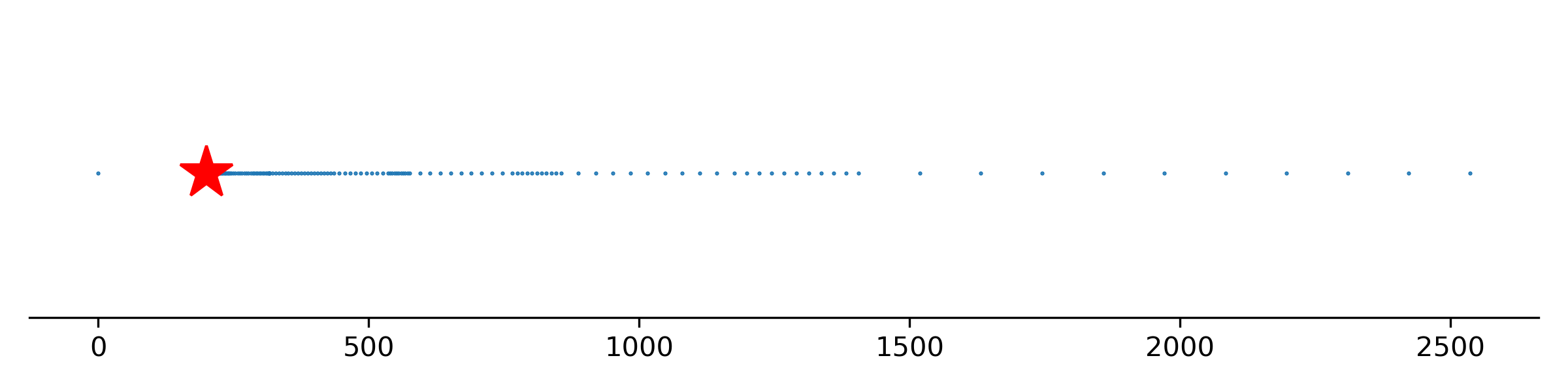

The above example, is yet another motivation to study and optimize routing algorithms specific to the appropriate objective/norm, as one solution cannot be good for all.
4 Optimal Routing of a Firefighter: a Combinatorial Algorithm
In this section we build upon the geometric partial-covering algorithm with good -trees to improve approximation bound for a specific norm, i.e., the Traveling Firefighter Problem.
We achieve the improved approximation bound by randomization (of parameter ) and optimization of the analysis w.r.t. approximation guarantee for a specific norm. This approach can provide approximation guarantees (better than ) for other TSP problems. We present main ideas in the rest of the section by proving Theorem 11.
Proof of Theorem 11.
We present a randomized approximation algorithm for general metrics, that can be efficiently de-randomized.
Among the set of good -trees, pre-computed for all using Lemma 17, let be the largest one of total length at most and let be a depth first traversal of that. Parameter is a constant, to be optimized for performance guarantees, and where is a random variable distributed uniformly over the interval Finally, we reverse each with probability half, and concatenate ’s (and shortcut repeated visits) to achieve the output ordering Let the latency of the th vertex visited by the optimal route be for some and integer
It is easy to see that the th sub-tour contains at least vertices, hence, we can bound
where is zero if the tour visits its th vertex before the th sub-tour, and depending on its location in the sub-tour. We can bound the expected damage, by
Bounding the expected damage at the th service, considering random variable we have
We can now choose in order to minimize the multiplicative bound
for an arbitrary , that can be achieved for for a small enough . With this we have
hence for an arbitrary . ∎
The above algorithm can be de-randomized by exploring all values for a dense enough quantization of or be simply used by repeating the randomized algorithm and reporting the best route.
4.1 Generalizing the Combinatorial Algorithm for TSP
The combinatorial algorithm from Section 4, stated as Algorithm 2, can be analyzed for arbitrary TSP; which for completeness we provide in this Section along with a proof of Theorem 12.
Theorem 18.
Algorithm 2 is a -approximation to TSP for all .
Proof.
Let the latency of the th vertex visited by the optimal route be
for some and integer . Let denote the latency of the th vertex visited by the algorithm. Following an argument similar to that in Theorem 22, it is enough to show that for all ,
for an appropriate constant to show that the algorithm is a approximation.
Note that , and so subtour contains at least vertices. If the tour visits the th vertex before the subtour , then
Otherwise, let be the distance of the th vertex from the starting vertex on one side of cycle . Therefore, the distance from the other side is at most . Since the cycle is traversed from each direction with equal probability, in this case
For fixed , this is maximum at or . And therefore, we have that
Taking expectation with respect to the random variable we have
Let . This is the same function we minimize in Theorem 22, and we have that
so that
This finishes the proof. ∎
5 Multi Vehicle TSP
In this Section we develop a Linear Programming approach that provides state-of-the-art approximation guarantees for single/multi vehicle TSP problems.
5.1 The Linear Programming Approach
We consider a natural linear programming relaxation of the TSP problem with vehicles, first introduced for a single vehicle TRP in [CS11] and then generalized to multiple vehicles TRP in [PS14]. Before we begin, let us assume that pairwise distances, hence time, are always integral and polynomially bounded, with for each edge , since quantization by rounding only adds a multiplicative error of to each edge and therefore results in an error of a factor at most for the length of any path in the graph.
For all and , let (resp. ) denote the set of all paths (resp. trees) of length at most rooted at vertex . The linear program seeks to select paths from at each time in and cover the vertices progressively, stopping once each vertex has been covered. For all and for all , variable indicates if vertex has been visited exactly at time by vehicle . For , variable indicates whether path has been selected at time (the maximum time can be upper bounded by , which as stated before can be assumed to be polynomially bounded). The objective function naturally is . One natural constraint is that each vertex be visited at least once (constraint (2)). Another natural constraint is that only one path from must be selected at time (constraint (3)). Finally, if vertex has been marked visited at some , must lie on some path selected at time (constraint (4)). We present the following linear programming relaxation using these constraints, denoted , along with its dual . Let denote its optimal value.
| subject to | (1) | ||||
| (2) | |||||
| (3) | |||||
| (4) | |||||
| subject to | (5) | ||||
| (6) | |||||
| (7) | |||||
5.2 Solving The LP
The above linear program has an exponential number of variables, and it is not known whether it can be solved directly. The next most natural line of attack – solving the dual – works here.
In the dual , separating over constraints (6) is straightforward since there are a polynomial number of variables and constraints involved. Constraints (7) have a combinatorial interpretation. Fix . Given rewards , is there some path rooted at of length at most (i.e., some path in ) with total reward on the path more than ? This is the decision problem version of the path-orienteering problem: given a starting vertex , some nonnegative rewards for the vertices, and some budget , one needs to determine the maximum reward a path starting at of length at most can gather.
Near-optimal approximations are known for the related tree-orienteering problem (see [CGRT03]). Consider the following relaxed version of the tree-orienteering problem: We are given nonnegative rewards for the vertices, a starting vertex , and an approximation parameter . Let the reward gathered by the optimal path for the path-orienteering problem with length budget be . Then, is there some tree rooted at of length at most (i.e., some tree in ) with total reward on the tree more than ? [CGRT03] design a polynomial time algorithm for determining gadgets called ‘good -tees’, and it also gives a polynomial-time algorithm for this version of the tree-orienteering problem using a reduction. To utilize this, we consider the following related LP (denoted and its dual, denoted ):
| subject to | ||||
| subject to | ||||
We still cannot separate the dual for this linear program using tree-orienteering. To utilize tree-orienteering, we need to introduce the parameter (where ) in the linear program. We denote this modification of as , and its dual is denoted .
| subject to | |||||
| (8) | |||||
| (9) | |||||
| (10) | |||||
| subject to | |||||
| (11) | |||||
| (12) | |||||
| (13) | |||||
Post and Swami [PS14] claim that for any , a feasible solution to of cost at most can be computed in polynomial time, using arguments analogous to those in Lemma 3.2 in [CS11]. We generalize their proof to arbitrary ; the proofs are similar, but we include it here for completeness.
Lemma 19.
Given any and , a feasible solution to can be found with cost at most .
Proof.
The main idea of the proof is to provide a modified separation oracle for the Ellipsoid algorithm. Recall that to solve linear programs over a polytope in polynomial time, the ellipsoid algorithm requires a polynomial time separation oracle that does the following: when a point is provided to the oracle, the oracle output either that (1) , or (2) gives a separating hyperplane such that but for all , (i.e., and lie on opposite sides of this hyperplane). Given this oracle, the ellipsoid algorithm in polynomial time either (1) outputs that , or (2) gives a feasible point in .
Now suppose we have another polytope such that . For any objective , . Let be an arbitrary function. Suppose we have a polynomial-time separation oracle that given a point , the oracle outputs either that (1) , or (2) gives a hyperplane separating and . Then, the ellipsoid algorithm in polynomial time either (1) outputs that , or (2) gives a feasible point in .
Let us first consider the relevant polytopes:
We give an oracle that given a and outputs either (1) a confirmation that or (2) a separating hyperplane for point and polytope . Since , the ellipsoid algorithm in polynomial time gives either (1) a confirmation that , or (2) a point in .
Using binary search, find the largest such that the ellipsoid algorithm gives a point in . Since is the largest value of such that is non-empty, this implies that . For each , the ellipsoid algorithm gives a confirmation that by giving an inconsistent subsystem of inequalities for . This subsystem has all inequalities from constraints (11), (13), and the inequality . It also contains only a polynomial number of inequalities from (12). By complementary slackness, we can get a solution to of cost at most with a polynomial number of nonzero variables. Choose to be small enough so that this cost is at most but large enough so that the algorithm is still polynomial time.
We describe the separation oracle now. Checking whether is easy, and if it is not true, can be output as a separating hyperplane between and . Similarly, each inequality in (11), (13) for can be checked individually and if does not satisfy any of those, that inequality can be output as a separating hyperplane between and . Since there are a polynomial number of these inequalities, this can be done in polynomial time.
It remains to check inequalities (12) for . To this end, for each , solve the relaxed version of the tree-orienteering problem with starting vertex , rewards , approximation parameter , and length budget to get a tree . has reward at least times the optimal reward for path-orienteering with length bound . If for some , the reward for exceeds , then as the separating hyperplane between and . Otherwise, all paths in gather reward at most , and therefore . This proves the correctness of the separation oracle and therefore finishes the proof. ∎
5.3 The Rounding Algorithm
Using Lemma 19, we generalize the LP-rounding algorithm of Post and Swami [PS14] for TRP (i.e., TSP) to TSP, achieving approximation algorithms for the TSP problem in general and TFP (i.e., -TSP) in particular, for both the single-vehicle and the multi-vehicle settings.
Let denote the optimal visit times for a given instance of the TSP problem with vehicles starting at vertices respectively, with the corresponding cost . Since is a relaxation for this problem, we have that the optimal cost for it, is at most . For any (that we fix later), using Lemma 19, obtain a solution to with cost at most . For convenience, denote , and . Therefore, we have that .
We give a randomized rounding algorithm (called LP-ROUND) with cost . The algorithm takes as input an the solution to . The fundamental idea for rounding is the same as that in [CGRT03] and [FTT21]: get exponentially large tours using trees with lengths bounded in terms of lengths of paths, except that instead of choosing good -trees, we choose trees using the solution . The major advantage this presents is that it is relatively easy to deal with the multi-vehicle case.
The analysis of the algorithm is somewhat involved and we introduce some notation to help. Let be the probability that vertex is not covered by the end of iteration . For convenience, define and for all . Observe that the probability that vertex is covered in iteration is . Also denote for all , and . When , we will omit the index corresponding to the vehicle in all variables.
We first need a recurrence relation for the probabilities .
Lemma 20.
- 1.
When , for arbitrary ,
- 2.
For an arbitrary and arbitrary ,
Proof.
- 1.
The probability that is visited in iteration is . Therefore,
- 2.
This is Lemma 5.3 of [PS14] and follows an argument similar to part 1. For completeness, we include the proof here. The probability that is visited by vehicle in iteration is
Therefore, . Now,
The first inequality is the AM-GM inequality, the second follows by convexity of , and the third is a standard bound for the exponential function. The result follows since for all .
∎
We define some additional terms that will help us bound in terms of for each vertex . Define for all . Denote
For all reals , let be the smallest such that , that is, . For a random variable , let denote the conditional expectation of for a fixed .
Lemma 21.
For each vertex ,
- 1.
,
- 2.
.
Proof.
- 1.
We first show that .
This helps determine in terms of . Suppose for some real and integer . Then, . Therefore, since where ,
Consequently, since , we have that
(14) - 2.
Suppose is covered in the th subtour for some vehicle . The cycle in iteration has length at most . Let be the distance of vertex from the starting vertex in one direction of the cycle . Then, the distance of from the starting vertex in the other direction of is at most . Since each direction is taken with probability , we have in this case that
For fixed , the right hand side is maximum at or , so that
Since the probability of vertex being covered in the th iteration is , the above implies that
∎
We are ready to present our main results. To warm up, let us first analyze the approximation bound for single vehicle case, providing matching guarantees to that of the combinatorial approach.
Theorem 22.
Given optimal solutions to , randomized rounding Algorithm 3 provides solutions that are
- 1.
-approximation for single-vehicle TFP,
- 2.
-approximation for single-vehicle TSP for any .
Proof.
We will show that for all ,
| (15) |
for an appropriate constant . As observed earlier, this implies that
By Markov’s inequality, for any constant ,
For , after independent runs of the rounding algorithm, the probability that in each run of the experiment is at most
Therefore, with high probability, after independent runs of the algorithm, there will be at least one run of the algorithm where
so that enough independent runs of LP-ROUND give a -approximation algorithm for TSP for all constants . This in particular implies that LP-ROUND is a -approximation for any , using an appropriate constant satisfying .
By Lemma 20 part (1) and the fact that , we have
Taking expectation in on both sides and using Lemma 21 part (1), we get that
Since
for each , there exists a such that
Therefore, for any given , we have some so that
That is, the constant in inequality (15) equals .
- 1.
. Given any , choose for a small enough so that . Finally, choose a small enough so that . This gives that ROUND is a -approximation to single-vehicle TFP.
- 2.
Arbitrary . Using an argument similar to part 1, it is enough to show that for all . We have
Choosing gives
It is easy to see that the minimum is not achieved at , so that the above inequality is strict, proving the claim.
∎
We end this section by proving the promised bounds for multi-vehicle problems.
Theorem 23.
Given optimal solutions to , the randomized rounding Algorithm 3 provides solutions that are
- 1.
-approximation for multi-vehicle TFP,
- 2.
-approximation for multi-vehicle TSP for all .
Proof.
Following the argument in Theorem 22, it is enough to show that for all , for an appropriate .
By Lemma 20 part (2) and the fact that , we have that
Therefore, the constant in inequality (15) equals .
- 1.
. Choose , so that . Choose small enough so that , giving that ROUND is a -approximation for multi-vehicle TSP.
- 2.
Arbitrary . Let . Using an argument similar to part 1, it is enough to show that .
Let ; we choose later. Then using , we have
Choose , so that . This proves the claim.
∎
We also remark that our reduction of TSP to Segmented-TSP can be generalized to multiple vehicles, with arbitrary start locations. Similar to the approach in Section 2 we can convert any optimal multi-vehicle solution to repetition of of prefix routes for each vehicle, all synchronized with a single , picked uniformly at random. Lemma 15 can be subsequently adapted to allow limiting the search space to solutions that have all vehicles at starting locations simultaneously at all , with negligible degrade of the optima. Finally, adapting the dynamic programming, we can guarantee a multiplicative loss given an (approximate) solver for multi-vehicle segmented TSP with constant deadlines, and the corresponding total number of destinations to be visited (by at least one vehicle) until up to each. This is indeed fruitful as results on segmented-TSP also generalize to multi-vehicle variant, e.g., in tree metric or Euclidean metric. Our algorithms can be similarly adapted in the case where release dates are added for the destinations.
6 Concluding Remarks
We studied combinatorial optimization problems whose objectives can be more appropriate, efficient, fair, and adjustable, depending on the enormous applications of optimal routing/scheduling. For TSP and TRP, the analyses of approximation algorithms as well as complexity results heavily rely on the linearity of the objective function. Hence, TFP and more generally TSP pose further challenging problems and require new techniques to be developed. We developed multiple techniques aimed towards high precision and/or scalable approximation of the optimal route.
We provided a high precision polynomial time reduction of TSP to segmented-TSP with only a constant number of deadlines for visiting the required number of destinations. Our reduction enables approximation schemes for TSP on Euclidean as well as weighted tree metrics; this is yet another motivation to further study the segmented-TSP problem.
Next, we investigated the case where we do not know what norm is the best to optimize, but want to be approximately optimal with respect to any. In this thread, we developed an algorithm for All-Norm TSP on general metrics with approximation factor . We also provided a first inapproximability result for All-Norm TSP.
We showed the kernel of our combinatorial algorithm can be optimized for performance with respect to a target norm, ensuring and approximations for TFP and TSP respectively.
Finally, with the combinatorial algorithms falling short of addressing the important multi-vehicle variants of our problems, we developed linear programming rounding techniques with first constant approximation bounds for multi-vehicle TSP and matching guarantees with the combinatorial approach for the single vehicle problems.
In the end, in addition to further improving the approximation bounds for the problems under study, we mention but a few of the potential directions to further expand this theory.
- •
Can TSP be reduced to sub-exponentially many instances of TSP, with constant degrade to the approximation factor? We believe not. 4 is much better than trying cases but still super-exponential.
- •
TSP, i.e., TRP is harder than TSP, at least on trees. For what is the TSP problem the hardest?
- •
Bounding the integrality gap of the linear programming relaxations remains critical.
- •
While TRP is strongly NP-hard on weighted trees, its complexity is unknown for caterpillars [Sit02]. Similarly complexity of TFP and TSP remain unresolved even on such special cases.
- •
While we theoretically claimed to be ideal for the Traveling Firefighter Problem, this suggestion should be given further justification / investigation in practice.
- •
- •
The impossibility bound for approximate All-Norm TSP and further NP-hardness of finding one can perhaps be improved.
References
- [ABCC06] David L Applegate, Robert E Bixby, Vasek Chvatal, and William J Cook, The traveling salesman problem: a computational study, Princeton university press, 2006.
- [ABHK11] Aaron Archer, MohammadHossein Bateni, MohammadTaghi Hajiaghayi, and Howard Karloff, Improved approximation algorithms for prize-collecting steiner tree and tsp, SIAM journal on computing 40 (2011), no. 2, 309–332.
- [ABK20] Gideon Amir, Rangel Baldasso, and Gady Kozma, The firefighter problem on polynomial and intermediate growth groups, Discrete Mathematics 343 (2020), no. 11, 112077.
- [ABL08] Giorgio Ausiello, Vincenzo Bonifaci, and Luigi Laura, The on-line asymmetric traveling salesman problem, Journal of Discrete Algorithms 6 (2008), no. 2, 290–298, Selected papers from CompBioNets 2004.
- [ABZ18] David Adjiashvili, Andrea Baggio, and Rico Zenklusen, Firefighting on trees beyond integrality gaps, ACM Transactions on Algorithms (TALG) 15 (2018), no. 2, 1–33.
- [ACP+86] Foto Afrati, Stavros Cosmadakis, Christos H Papadimitriou, George Papageorgiou, and Nadia Papakostantinou, The complexity of the travelling repairman problem, RAIRO-Theoretical Informatics and Applications 20 (1986), no. 1, 79–87.
- [AERW04] Yossi Azar, Leah Epstein, Yossi Richter, and Gerhard J Woeginger, All-norm approximation algorithms, Journal of Algorithms 52 (2004), no. 2, 120–133.
- [AGGP21] Yossi Azar, Arun Ganesh, Rong Ge, and Debmalya Panigrahi, Online service with delay, ACM Transactions on Algorithms 17 (2021), no. 3.
- [AK00] Sanjeev Arora and George Karakostas, A approximation algorithm for the k-MST problem, Proceedings of the 11th Annual ACM-SIAM Symposium on Discrete Algorithms, 2000, pp. 754–759.
- [ALMS00] Giorgio Ausiello, Stefano Leonardi, and Alberto Marchetti-Spaccamela, On salesmen, repairmen, spiders, and other traveling agents, Italian Conference on Algorithms and Complexity, Springer, 2000, pp. 1–16.
- [ALW08] Aaron Archer, Asaf Levin, and David P Williamson, A faster, better approximation algorithm for the minimum latency problem, SIAM Journal on Computing 37 (2008), no. 5, 1472–1498.
- [AW03] Aaron Archer and David P Williamson, Faster approximation algorithms for the minimum latency problem, Proceedings of the fourteenth annual ACM-SIAM symposium on Discrete algorithms, Society for Industrial and Applied Mathematics, 2003, pp. 88–96.
- [BBFT21] Nikhil Bansal, Jatin Batra, Majid Farhadi, and Prasad Tetali, Improved approximations for min sum vertex cover and generalized min sum set cover, Proceedings of the 2021 ACM-SIAM Symposium on Discrete Algorithms (SODA), SIAM, 2021, pp. 998–1005.
- [BC11] Sylvia Boyd and Robert Carr, Finding low cost TSP and 2-matching solutions using certain half-integer subtour vertices, Discrete Optimization 8 (2011), no. 4, 525–539.
- [BCC+94] Avrim Blum, Prasad Chalasani, Don Coppersmith, Bill Pulleyblank, Prabhakar Raghavan, and Madhu Sudan, On the minimum latency problem, Proceedings of the twenty-sixth annual ACM symposium on Theory of computing, pages 163–171. ACM (1994).
- [BKL21] Marcin Bienkowski, Artur Kraska, and Hsiang-Hsuan Liu, Traveling repairperson, unrelated machines, and other stories about average completion times, arXiv preprint arXiv:2102.06904 (2021).
- [Bor19] Alejandra Borunda, See how much of the Amazon forest is burning, how it compares to other years, National Geographic (2019).
- [BP90] Sylvia C Boyd and William R Pulleyblank, Optimizing over the subtour polytope of the travelling salesman problem, Mathematical programming 49 (1990), no. 1-3, 163–187.
- [BP03] Nikhil Bansal and Kirk Pruhs, Server scheduling in the lp norm: a rising tide lifts all boat, Proceedings of the thirty-fifth annual ACM symposium on Theory of computing, 2003, pp. 242–250.
- [CGRT03] Kamalika Chaudhuri, Brighten Godfrey, Satish Rao, and Kunal Talwar, Paths, trees, and minimum latency tours, 44th Annual IEEE Symposium on Foundations of Computer Science, 2003. Proceedings., IEEE, 2003, pp. 36–45.
- [Chr76] Nicos Christofides, Worst-case analysis of a new heuristic for the Travelling Salesman Problem, Tech. Report RR-388, February 1976.
- [CJJ20] T.-H. Hubert Chan, Haotian Jiang, and Shaofeng H.-C. Jiang, A unified ptas for prize collecting tsp and steiner tree problem in doubling metrics, ACM Transactions on Algorithms 16 (2020), no. 2.
- [CKP12] Chandra Chekuri, Nitish Korula, and Martin Pál, Improved algorithms for orienteering and related problems, ACM Transactions on Algorithms (TALG) 8 (2012), no. 3, 1–27.
- [CS11] Deeparnab Chakrabarty and Chaitanya Swamy, Facility location with client latencies: linear-programming based techniques for minimum latency problems, 15th IPCO, 2011, pp. 92–103.
- [CS18] Deeparnab Chakrabarty and Chaitanya Swamy, Interpolating between k-median and k-center: Approximation algorithms for ordered k-median, ICALP, vol. 45, 2018, pp. 29:1–29:14.
- [CV00] Robert Carr and Santosh Vempala, Towards a 4/3 approximation for the asymmetric traveling salesman problem, 116–125.
- [DFH21] Arye Deutch, Ohad Noy Feldheim, and Rani Hod, Multi-layered planar firefighting, arXiv preprint arXiv:2105.03759 (2021).
- [EG03] Matthias Ehrgott and Xavier Gandibleux, Multiple objective combinatorial optimization — a tutorial, Multi-Objective Programming and Goal Programming (Berlin, Heidelberg), Springer Berlin Heidelberg, 2003, pp. 3–18.
- [FLM93] Matteo Fischetti, Gilbert Laporte, and Silvano Martello, The delivery man problem and cumulative matroids, Operations Research 41 (1993), no. 6, 1055–1064.
- [FLT04] Uriel Feige, László Lovász, and Prasad Tetali, Approximating min sum set cover, Algorithmica 40 (2004), no. 4, 219–234.
- [FM09] Stephen Finbow and Gary MacGillivray, The firefighter problem: a survey of results, directions and questions., Australas. J Comb. 43 (2009), 57–78.
- [FTT21] Majid Farhadi, Alejandro Toriello, and Prasad Tetali, The traveling firefighter problem, SIAM Conference on Applied and Computational Discrete Algorithms (ACDA21), SIAM, 2021, pp. 205–216.
- [Gar96] Naveen Garg, A 3-approximation for the minimum tree spanning k vertices, Proceedings of 37th Conference on Foundations of Computer Science, IEEE, 1996, pp. 302–309.
- [GGKT08] Daniel Golovin, Anupam Gupta, Amit Kumar, and Kanat Tangwongsan, All-norms and all--norms approximation algorithms, IARCS Annual Conference on Foundations of Software Technology and Theoretical Computer Science, Schloss Dagstuhl-Leibniz-Zentrum für Informatik, 2008.
- [GK98] Michel Goemans and Jon Kleinberg, An improved approximation ratio for the minimum latency problem, Mathematical Programming 82 (1998), no. 1-2, 111–124.
- [GLS05] David Gamarnik, Moshe Lewenstein, and Maxim Sviridenko, An improved upper bound for the TSP in cubic 3-edge-connected graphs, Operations Research Letters 33 (2005), no. 5, 467–474.
- [Goe95] Michel X Goemans, Worst-case comparison of valid inequalities for the TSP, Mathematical Programming 69 (1995), no. 1-3, 335–349.
- [Har95] Bert Hartnell, Firefighter! an application of domination, the 24th Manitoba Conference on Combinatorial Mathematics and Computing, University of Minitoba, Winnipeg, Cadada, 1995, 1995.
- [Har04] Stephen G Hartke, Attempting to narrow the integrality gap for the firefighter problem on trees., Discrete Methods in Epidemiology, 2004, pp. 225–231.
- [HLP88] GH Hardy, JE Littlewood, and G Polya, Inequalities, Cambridge University Press (1988).
- [HNR19] Arash Haddadan, Alantha Newman, and R Ravi, Shorter tours and longer detours: uniform covers and a bit beyond, Mathematical Programming (2019), 1–29.
- [Hoo18] K Hoover, Wildfire statistics congressional research service, 2018.
- [IS20] Sharat Ibrahimpur and Chaitanya Swamy, Approximation algorithms for stochastic minimum-norm combinatorial optimization, Annual Symposium on Foundations of Computer Science (FOCS), vol. 61, 2020, pp. 966–977.
- [JHC19] Sirine Jmal, Boukthir Haddar, and Habib Chabchoub, Apply the quantum particle swarm optimization for the k-traveling repairman problem, Soft Computing 23 (2019), no. 23, 12547–12560.
- [KKG20] Anna R Karlin, Nathan Klein, and Shayan Oveis Gharan, A (slightly) improved approximation algorithm for metric TSP, arXiv preprint arXiv:2007.01409 (2020).
- [KLL14] Rolf Klein, Christos Levcopoulos, and Andrzej Lingas, Approximation algorithms for the geometric firefighter and budget fence problems, Latin American Symposium on Theoretical Informatics, Springer, 2014, pp. 261–272.
- [KLS15] Marek Karpinski, Michael Lampis, and Richard Schmied, New inapproximability bounds for tsp, Journal of Computer and System Sciences 81 (2015), no. 8, 1665–1677.
- [KP20] Miroslav Kulich and Libor Preucil, Multi-robot search for a stationary object placed in a known environment.
- [KPY96] Elias Koutsoupias, Christos Papadimitriou, and Mihalis Yannakakis, Searching a fixed graph, International Colloquium on Automata, Languages, and Programming, Springer, 1996, pp. 280–289.
- [KRT99] Jon Kleinberg, Yuval Rabani, and Éva Tardos, Fairness in routing and load balancing, 40th Annual Symposium on Foundations of Computer Science (Cat. No. 99CB37039), IEEE, 1999, pp. 568–578.
- [LWH+19] Chuanwen Luo, Yongcai Wang, Yi Hong, Wenping Chen, Xingjian Ding, Yuqing Zhu, and Deying Li, Minimizing data collection latency with unmanned aerial vehicle in wireless sensor networks, Journal of Combinatorial Optimization 38 (2019), no. 4, 1019–1042.
- [MDZL08] Isabel Méndez-Díaz, Paula Zabala, and Abilio Lucena, A new formulation for the traveling deliveryman problem, Discrete applied mathematics 156 (2008), no. 17, 3223–3237.
- [Min89] Edward Minieka, The delivery man problem on a tree network, Annals of Operations Research 18 (1989), no. 1, 261–266.
- [NAS] Fire information for resource management system, nasa, https://firms.modaps.eosdis.nasa.gov.
- [PFF+20] Alice Paul, Daniel Freund, Aaron Ferber, David B Shmoys, and David P Williamson, Budgeted prize-collecting traveling salesman and minimum spanning tree problems, Mathematics of Operations Research 45 (2020), no. 2, 576–590.
- [PS14] Ian Post and Chaitanya Swamy, Linear programming-based approximation algorithms for multi-vehicle minimum latency problems, Proceedings of the Twenty-Sixth Annual ACM-SIAM Symposium on Discrete Algorithms, SIAM, 2014, pp. 512–531.
- [PY93] Christos H Papadimitriou and Mihalis Yannakakis, The traveling salesman problem with distances one and two, Mathematics of Operations Research 18 (1993), no. 1, 1–11.
- [Ser78] AI Serdyukov, O nekotorykh ekstremal’nykh obkhodakh v grafakh, Upravlyayemyye sistemy 17 (1978), 76–79.
- [Sit02] René Sitters, The minimum latency problem is NP-hard for weighted trees, International conference on integer programming and combinatorial optimization, Springer, 2002, pp. 230–239.
- [Sit14] , Polynomial time approximation schemes for the traveling repairman and other minimum latency problems., Proceedings of the twenty-fifth annual ACM-SIAM symposium on Discrete algorithms, SIAM, 2014, pp. 604–616.
- [Sit21] , Polynomial time approximation schemes for the traveling repairman and other minimum latency problems, SIAM Journal on Computing 50 (2021), no. 5, 1580–1602.
- [SW90] David B Shmoys and David P Williamson, Analyzing the held-karp TSP bound: A monotonicity property with application, Information Processing Letters 35 (1990), no. 6, 281–285.
- [SWVZ12] Frans Schalekamp, David P Williamson, and Anke Van Zuylen, A proof of the Boyd-Carr conjecture, Proceedings of the twenty-third annual ACM-SIAM symposium on Discrete Algorithms, SIAM, 2012, pp. 1477–1486.
- [TCM20] Guy Tennenholtz, Constantine Caramanis, and Shie Mannor, Sequential vaccination for containing epidemics, medRxiv (2020).
- [TVZ20] Vera Traub, Jens Vygen, and Rico Zenklusen, Reducing path TSP to TSP, Proceedings of the 52nd Annual ACM SIGACT Symposium on Theory of Computing, 2020, pp. 14–27.
- [WGZ+21] Daoping Wang, Dabo Guan, Shupeng Zhu, Michael Mac Kinnon, Guannan Geng, Qiang Zhang, Heran Zheng, Tianyang Lei, Shuai Shao, Peng Gong, et al., Economic footprint of california wildfires in 2018, Nature Sustainability 4 (2021), no. 3, 252–260.
- [Wil94] Todd Gerald Will, Extremal results and algorithms for degree sequences of graphs.
- [Wol80] Laurence A Wolsey, Heuristic analysis, linear programming and branch and bound, Combinatorial Optimization II, Springer, 1980, pp. 121–134.
- [XZL20] Mingyu Xiao, Jianan Zhang, and Weibo Lin, Parameterized algorithms and complexity for the traveling purchaser problem and its variants, Journal of Combinatorial Optimization (2020).
- [ZTXL15] Huili Zhang, Weitian Tong, Yinfeng Xu, and Guohui Lin, The steiner traveling salesman problem with online edge blockages, European Journal of Operational Research 243 (2015), no. 1, 30–40.
Appendix A All-Norm Inapproximability Example
Our example for inapproximability of All-Norm TSP has similar structure as the exponential sequence presented in Section 3, and is computationally tuned and verified. This suggests the best (worst) example may have a different structure. We present the locations of the destinations in to be visited by a traveler who is starting at . It was previously presented as Figure 3.