跳到论文正文
W Papers独立论文阅读器 arXiv:2208.04065 论文正文 计算阅读时间 · 0%
引用这篇论文根据当前论文元数据生成,正式投稿前建议核对。


License: arXiv.org perpetual non-exclusive license
arXiv:2208.04065v1 [math.OC] 08 Aug 2022

2022

This paper proposes a new family of algorithms for the online optimisation of composite objectives. The algorithms can be interpreted as the combination of the exponentiated gradient and pp-norm algorithm. Combined with algorithmic ideas of adaptivity and optimism, the proposed algorithms achieve a sequence-dependent regret upper bound, matching the best-known bounds for sparse target decision variables. Furthermore, the algorithms have efficient implementations for popular composite objectives and constraints and can be converted to stochastic optimisation algorithms with the optimal accelerated rate for smooth objectives.

Optimistic Optimisation of Composite Objective with Exponentiated Update

Weijia Shao Email: weijia.shao@campus.tu-berlin.de Affiliation: Faculty of Electrical Engineering and Computer Science, Technische Universität Berlin, Ernst-Reuter-Platz 7, Berlin, 10587, Germany    Fikret Sivrikaya Email: fikret.sivrikaya@gt-arc.com Affiliation:  GT-ARC Gemeinnützige GmbH, Ernst-Reuter-Platz 7, Berlin, 10587, Germany    Sahin Albayrak Email: sahin.albayrak@dai-labor.de Affiliation: Faculty of Electrical Engineering and Computer Science, Technische Universität Berlin, Ernst-Reuter-Platz 7, Berlin, 10587, Germany Affiliation:  GT-ARC Gemeinnützige GmbH, Ernst-Reuter-Platz 7, Berlin, 10587, Germany
keywords
Exponetiated Gradient, Composite Objective, Online Convex Optimisation, Sparsity

1 Introduction

Many machine learning problems involve minimising high dimensional composite objectives (Lu \BOthers. \APACyear2014; Ribeiro \BOthers. \APACyear2016; Dhurandhar \BOthers. \APACyear2018; Xie \BOthers. \APACyear2018). For example, in the task of explaining predictions of an image classifier (Ribeiro \BOthers. \APACyear2016; Dhurandhar \BOthers. \APACyear2018), we need to find a sufficiently small set of features explaining the prediction by solving the following constrained optimisation problem

minx∈ℝdl⁡(x)+λ1​∥x∥1+λ22​∥x∥22s.t.|xi|≤ci for all i=1,…,d,\begin{split}\min_{x\in\mathbb{R}^{d}}\quad&l(x)+\lambda_{1}\lVert x\rVert_{1}+\frac{\lambda_{2}}{2}\lVert x\rVert_{2}^{2}\\ \ \textrm{s.t.}\quad&|x_{i}\rvert\leq c_{i}\textrm{ for all }i=1,\ldots,d,\\ \end{split}

where ll is a function relating to the classifier, λ1\lambda_{1} controls the sparsity of the feature set, λ2\lambda_{2} controls the complexity of the feature set, and c1,…,cdc_{1},\ldots,c_{d} are the ranges of the features. For ll with a complicated structure and large dd, it is practical to solve the problem by optimising the first-order approximation of the objective function (Lan \APACyear2020). However, the first-order methods can not attain optimal performance due to the non-smooth component λ1​∥⋅∥1\lambda_{1}\lVert\cdot\rVert_{1}. Furthermore, the purpose of introducing the ℓ1\ell_{1} regularisation is to ensure the sparsity of the decision variable. Applying the first-order algorithms directly on the subgradient of λ1​∥⋅∥1\lambda_{1}\lVert\cdot\rVert_{1} does not lead to sparse updates (J.C. Duchi \BOthers. \APACyear2010). We refer to the objective function consisting of a loss with a complicated structure and a simple (possibly non-smooth) convex regularisation term as a composite objective.

This paper focuses on the more general online convex optimisation (OCO), which can be considered as an iterative game between a player and an adversary. In each round tt of the game, the player makes a decision xt∈𝒦x_{t}\in\mathcal{K}. Next, the adversary selects and reveals a convex loss ltl_{t} to the player, who then suffers the composite loss ft​(x)=lt​(x)+rt​(x)f_{t}(x)=l_{t}(x)+r_{t}(x), where lt:𝒦→ℝl_{t}:\mathcal{K}\to\mathbb{R} is a convex function revealed at each iteration and rt:𝕏→ℝ≥0r_{t}:\mathbb{X}\to\mathbb{R}_{\geq 0} is a known closed convex function. The target is to develop algorithms minimising the regret of not choosing the best decision x∈𝒦x\in\mathcal{K}

ℛ1:T=∑t=1Tft(xt)−minx∈𝒦∑t=1Tft(x).\mathcal{R}_{1:T}=\sum_{t=1}^{T}f_{t}(x_{t})-\min_{x\in\mathcal{K}}\sum_{t=1}^{T}f_{t}(x).

An online optimisation algorithm can be converted into a stochastic optimisation algorithm using the online-to-batch conversion technique (Cesa-Bianchi \BOthers. \APACyear2004), which is our primary motivation. In addition to that, online optimisation also has many direct applications, such as recommender systems (Song \BOthers. \APACyear2014) and time series prediction (Anava \BOthers. \APACyear2013).

Given a sequence of subgradients {gt}\{g_{t}\} of {lt}\{l_{t}\}, we are interested in the so-called adaptive algorithms ensuring regret bounds of the form 𝒪⁡(∑t=1T∥gt∥∗2)\mathcal{O}(\sqrt{\sum_{t=1}^{T}\lVert g_{t}\rVert_{*}^{2}}). The adaptive algorithms are worst-case optimal in the online setting (McMahan \BBA Streeter \APACyear2010) and can be converted into stochastic optimisation algorithms with optimal convergence rates (Levy \BOthers. \APACyear2018; Kavis \BOthers. \APACyear2019; Cutkosky \APACyear2019; Joulani \BOthers. \APACyear2020). The adaptive subgradient methods (AdaGrad) (J. Duchi \BOthers. \APACyear2011) and their variants (J. Duchi \BOthers. \APACyear2011; Orabona \BOthers. \APACyear2015; Orabona \BBA Pál \APACyear2018; Alacaoglu \BOthers. \APACyear2020) have become the most popular adaptive algorithms in recent years. They are often applied to estimating deep learning models and outperform standard optimisation algorithms when the gradient vectors are sparse. However, such property can not be expected in every problem. If the decision variables are in an ℓ1\ell_{1} ball and gradient vectors are dense, the Adagrad-style algorithms do not have an optimal theoretical guarantee due to the sub-linear regret dependence on the dimensionality.

The exponentiated gradient (EG) methods (Kivinen \BBA Warmuth \APACyear1997; Arora \BOthers. \APACyear2012), which are designed for estimating weights in the positive orthant, enjoy the regret bound growing logarithmically with the dimensionality. The EG±\operatorname{\textbf{EG}^{\pm}} algorithm generalises this idea to negative weights (Kivinen \BBA Warmuth \APACyear1997; Warmuth \APACyear2007). Given dd dimensional problems with the maximum norm of the gradient bounded by GG, the regret of EG±\operatorname{\textbf{EG}^{\pm}} is upper bounded by 𝒪⁡(G​T​ln⁡d)\mathcal{O}(G\sqrt{T\ln d}). As the performance of the EG±\operatorname{\textbf{EG}^{\pm}} algorithm depends strongly on the choice of hyperparameters, the pp-norm algorithm (Gentile \APACyear2003), which is less sensitive to the tuning of hyperparameters, is introduced to approach the logarithmic behaviour of EG±\operatorname{\textbf{EG}^{\pm}}. Kakade \BOthers. \APACyear2012 further extends the pp-norm algorithm to learning with matrices. An adaptive version of the pp-norm algorithm is analysed in Orabona \BOthers. \APACyear2015, which has a regret upper bound proportional to ∥x∥p,∗2​∑t=1T∥gt∥p2\lVert x\rVert_{p,*}^{2}\sqrt{\sum_{t=1}^{T}\lVert g_{t}\rVert_{p}^{2}} for a given sequence of gradients {gt}\{g_{t}\}. By choosing p=2​ln⁡dp=2\ln d, a regret upper bound 𝒪⁡(∥x∥12​ln⁡d​∑t=1T∥gt∥∞2)\mathcal{O}(\lVert x\rVert_{1}^{2}\sqrt{\ln d\sum_{t=1}^{T}\lVert g_{t}\rVert_{\infty}^{2}}) can be achieved. However, tuning hyperparameters is still required to attain the optimal regret 𝒪⁡(∥x∥1​ln⁡d​∑t=1T∥gt∥∞2)\mathcal{O}(\lVert x\rVert_{1}\sqrt{\ln d\sum_{t=1}^{T}\lVert g_{t}\rVert_{\infty}^{2}}).

Recently, Ghai \BOthers. \APACyear2020 has introduced a hyperbolic regulariser for online mirror descent update (HU), which can be viewed as an interpolation between gradient descent and EG. It has a logarithmic behaviour as in EG and a stepsize that can be flexibly scheduled as gradient descent. However, many optimisation problems with sparse targets have an ℓ1\ell_{1} or nuclear regulariser in the objective function. Otherwise, the optimisation algorithm has to pick a decision variable from a compact decision set. Due to the hyperbolic regulariser, it is difficult to derive a closed-form solution for either case. Ghai \BOthers. \APACyear2020 has proposed a workaround by tuning a temperature-like hyperparameter to normalise the decision variable at each iteration, which is equivalent to the EG±\operatorname{\textbf{EG}^{\pm}} algorithm and leads to a performance dependence on the tuning.

This paper proposes a family of algorithms for the online optimisation of composite objectives. The algorithms employ an entropy-like regulariser combined with algorithmic ideas of adaptivity and optimism. Equipped with the regulariser, the online mirror descent (OMD) and the follow-the-regulariser-leader (FTRL) algorithms update the absolute value of the scalar components of the decision variable in the same way as EG in the positive orthant. The directions of the decision variables are set in the same way as the pp-norm algorithm. To derive the regret upper bound, we first show that the regulariser is strongly convex with respect to the ℓ1\ell_{1}-norm over the ℓ1\ell_{1} ball. Then we analyse the algorithms in the comprehensive framework for optimistic algorithms with adaptive regularisers (Joulani \BOthers. \APACyear2017). Given the radius of decision set DD, sequences of gradients {gt}\{g_{t}\} and hints {ht}\{h_{t}\}, the proposed algorithms achieve a regret upper bound in the form of 𝒪⁡(D​ln⁡d​∑t=1T∥gt−ht∥∞2)\mathcal{O}(D\sqrt{\ln d\sum_{t=1}^{T}\lVert g_{t}-h_{t}\rVert^{2}_{\infty}}). With the techniques introduced in Ghai \BOthers. \APACyear2020, a spectral analogue of the entropy-like regulariser can be found and proved to be strongly convex with respect to the nuclear norm over the nuclear ball, from which the best-known regret upper bound depending on ln⁡(min⁡{m,n})\sqrt{\ln(\min\{m,n\})} for problems in ℝm,n\mathbb{R}^{m,n} follows.

Furthermore, the algorithms have closed-form solutions for the ℓ1\ell_{1} and nuclear regularised objective functions. For the ℓ2\ell_{2} and Frobenius regularised objectives, the update rules involve values of the principal branch of the Lambert function, which can be well approximated. We propose a sorting based procedure projecting the solution to the decision set for the ℓ1\ell_{1} or nuclear ball constrained problems. Finally, the proposed online algorithms can be converted into algorithms for stochastic optimisation with the technique introduced in Joulani \BOthers. \APACyear2020. We show that the converted algorithms guarantee an optimal accelerated convergence rate for smooth objective functions. The convergence rate depends logarithmically on the dimensionality of the problem, which suggests its advantage compared to the accelerated AdaGrad-Style algorithms (Levy \BOthers. \APACyear2018; Cutkosky \APACyear2019; Joulani \BOthers. \APACyear2020).

The rest of the paper is organised as follows. Section 2 reviews the existing work. Section 3 introduces the notation and preliminary concepts. Next, we present and analyse our algorithms in Section 4. In Section 5, we derive efficient implementations for some popular choices of composite objectives, constraints and stochastic optimisation. Section 6 demonstrates the empirical evaluations using both synthetic and real-world data. Finally, we conclude our work in Section 7.

2 Related Work

Our primary motivation is to solve the optimisation problems with an elastic net regulariser in their objective function, which are highly involved in attacking (Carlini \BBA Wagner \APACyear2017; P\BHBIY. Chen \BOthers. \APACyear2018; Cancela \BOthers. \APACyear2021) and explaining (Dhurandhar \BOthers. \APACyear2018; Ribeiro \BOthers. \APACyear2016) deep neural networks. The proximal gradient method (PGD) (Nesterov \APACyear2003) and its accelerated variants (Beck \BBA Teboulle \APACyear2009) are usually applied to solving the problem. However, these algorithms are not practical since they require prior knowledge about the smoothness of the objective function to ensure their convergence.

The AdaGrad-style algorithms (J. Duchi \BOthers. \APACyear2011; Orabona \BOthers. \APACyear2015; Orabona \BBA Pál \APACyear2018; Alacaoglu \BOthers. \APACyear2020) have become popular in the machine learning community in recent years. Given the gradient vectors g1,…,gtg_{1},\ldots,g_{t} received at iteration tt, the core idea of these algorithms is to set the stepsizes proportional to 1∑s=1t−1∥gs∥∗2\frac{1}{\sqrt{\sum_{s=1}^{t-1}\lVert g_{s}\rVert_{*}^{2}}} to ensure a regret upper bounded by 𝒪⁡(∑t=1T∥gt∥∗2)\mathcal{O}(\sqrt{\sum_{t=1}^{T}\lVert g_{t}\rVert_{*}^{2}}) after TT iterations. Online learning algorithms with this adaptive regret can be directly applied to the stochastic optimisation problems (Li \BBA Orabona \APACyear2019; Alacaoglu \BOthers. \APACyear2020) or can be converted into a stochastic algorithm (Cesa-Bianchi \BBA Gentile \APACyear2008) with a convergence rate 𝒪⁡(1T)\mathcal{O}(\frac{1}{\sqrt{T}}). This rate can be further improved to 𝒪⁡(1T2)\mathcal{O}(\frac{1}{T^{2}}) for unconstrained problems with smooth loss functions by applying the acceleration techniques (Levy \BOthers. \APACyear2018; Kavis \BOthers. \APACyear2019; Cutkosky \APACyear2019). These acceleration techniques do not require prior knowledge about the smoothness of the loss function and a guarantee convergence rate of 𝒪⁡(1T)\mathcal{O}(\frac{1}{\sqrt{T}}) for non-smooth functions. Joulani \BOthers. \APACyear2020 has proposed a simple approach to accelerate optimistic online optimisation algorithms with adaptive regret bound.

Given a dd-dimensional problem, the algorithms mentioned above have a regret upper bound depending (sub-) linearly on dd. We are interested in a logarithmic regret dependence on the dimensionality, which can be attained by the EG family algorithms (Kivinen \BBA Warmuth \APACyear1997; Warmuth \APACyear2007; Arora \BOthers. \APACyear2012) and their adaptive optimistic extension (Steinhardt \BBA Liang \APACyear2014). However, these algorithms work only for decision sets in the form of cross-polytopes and require prior knowledge about the radius of the decision set for general convex optimisation problems. The pp-norm algorithm (Gentile \APACyear2003; Kakade \BOthers. \APACyear2012) does not have the limitation mentioned above; however, it still requires prior knowledge about the problem to attain optimal performance (Orabona \BOthers. \APACyear2015). The HU algorithm (Ghai \BOthers. \APACyear2020), which interpolates gradient descent and EG, can theoretically be applied to loss functions with elastic net regularisers and decision sets other than cross-polytopes. However, it is not practical due to the complex projection step.

Following the idea of HU, we propose more practical algorithms interpolating EG and the pp-norm algorithm. The core of our algorithm is a symmetric logarithmic function. Orabona \APACyear2013 first introduced the idea of composing the single-dimensional symmetric logarithmic function and a norm to generalise EG to the infinite-dimensional space. It has become popular for parameter-free optimisation (Cutkosky \BBA Boahen \APACyear2016; Cutkosky \BBA Boahen \APACyear2017\APACexlab\BCnt1; Cutkosky \BBA Boahen \APACyear2017\APACexlab\BCnt2; Kempka \BOthers. \APACyear2019) since one can easily construct an adaptive regulariser with this composition (Cutkosky \BBA Boahen \APACyear2017\APACexlab\BCnt1). In this paper, instead of using the composition, we apply the symmetric logarithmic function directly to each entry of a vector to construct a symmetric entropy-like function that is strongly convex with respect to the ℓ1\ell_{1} norm. We analyse MD and FTRL with the entropy-like function in the framework developed in Joulani \BOthers. \APACyear2017. The analysis of the spectral analogue of the entropy-like function follows the idea proposed in Ghai \BOthers. \APACyear2020.

3 Preliminary

The focus of this paper is OCO with the decision variable taken from a compact convex subset 𝒦⊆𝕏\mathcal{K}\subseteq\mathbb{X} of finite dimensional vector space equipped with a norm ∥⋅∥\lVert\cdot\rVert. Given a sequence of vectors {vt}\{v_{t}\}, we use the compressed-sum notation v1:t=∑s=1tvsv_{1:t}=\sum_{s=1}^{t}v_{s} for simplicity. We denote by 𝕏∗\mathbb{X}_{*} the dual space with the dual norm ∥⋅∥∗\lVert\cdot\rVert_{*}. The bi-linear map combining vectors in 𝕏∗\mathbb{X}_{*} and 𝕏\mathbb{X} is denoted by

⟨⋅,⋅⟩:𝕏∗×𝕏→ℝ,(θ,x)↦θ​x.\langle\cdot,\cdot\rangle:\mathbb{X}_{*}\times\mathbb{X}\to\mathbb{R},(\theta,x)\mapsto\theta x.

For 𝕏=ℝd\mathbb{X}=\mathbb{R}^{d}, we denote by ∥⋅∥1\lVert\cdot\rVert_{1} the ℓ1\ell_{1} norm, the dual norm of which is the maximum norm denoted by ∥⋅∥∞\lVert\cdot\rVert_{\infty}. It is well known that the ℓ2\ell_{2} norm denoted by ∥⋅∥2\lVert\cdot\rVert_{2} is self-dual. In case 𝕏\mathbb{X} is the space of the matrices, for simplicity, we also use ∥⋅∥1\lVert\cdot\rVert_{1}, ∥⋅∥2\lVert\cdot\rVert_{2} and ∥⋅∥∞\lVert\cdot\rVert_{\infty} for the nuclear, Frobenius and spectral norm, respectively.

Let σ:ℝm,n→ℝmin⁡{m,n}\sigma:\mathbb{R}^{m,n}\to\mathbb{R}^{\min\{m,n\}} be the function mapping a matrix to its singular values. Define

diag:ℝmin⁡{m,n}→ℝm,n,x↦X\operatorname{diag}:\mathbb{R}^{\min\{m,n\}}\to\mathbb{R}^{m,n},x\mapsto X

with

Xi​j={xi,if ​i=j0,otherwise.X_{ij}=\begin{cases}x_{i},&\text{if }i=j\\ 0,&\text{otherwise}.\\ \end{cases}

Clearly, the singular value decomposition (SVD) of a matrix XX can be expressed as

X=U​diag⁡(σ⁡(X))​V⊤.X=U\operatorname{diag}(\sigma(X))V^{\top}.

Similarly, we write the eigendecomposition of a symmetric matrix XX as

X=U​diag⁡(λ⁡(X))​U⊤,X=U\operatorname{diag}(\lambda(X))U^{\top},

where we denote by λ:𝕊d↦ℝd\lambda:\mathbb{S}^{d}\mapsto\mathbb{R}^{d} the function mapping a symmetric matrix to its spectrum.

Given a convex set 𝒦⊆𝕏\mathcal{K}\subseteq\mathbb{X} and a convex function f:𝒦→ℝf:\mathcal{K}\to\mathbb{R} defined on 𝒦\mathcal{K}, we denote by ∂f(y)={g∈𝕏∗|∀y∈𝒦.f(x)−f(y)≥⟨g,x−y⟩}\partial f(y)=\{g\in\mathbb{X}_{*}\lvert\forall y\in\mathcal{K}.f(x)-f(y)\geq\langle g,x-y\rangle\} the subgradient of ff at yy. We refer to ▽​f​(y)\triangledown f(y) any element in ∂f⁡(y)\partial f(y). A function is η\eta-strongly convex with respect to ∥⋅∥\lVert\cdot\rVert over 𝒦\mathcal{K} if

f⁡(x)−f⁡(y)≥⟨▽​f​(y),x−y⟩+η2​∥x−y∥2f(x)-f(y)\geq\langle\triangledown f(y),x-y\rangle+\frac{\eta}{2}\lVert x-y\rVert^{2}

holds for all x,y∈𝒦x,y\in\mathcal{K} and ▽​f​(y)∈∂f⁡(y)\triangledown f(y)\in\partial f(y).

4 Algorithms and Analysis

In this section, we present and analyse our algorithms, which begins with a short review on EG and the pp-norm algorithm for the case ft=ltf_{t}=l_{t}. The EG algorithm can be considered as an instance of OMD, the update rules of which is given by

xt+1,i∝exp⁡(ln⁡(xt,i)−1η​gt,i),x_{t+1,i}\propto\exp(\ln(x_{t,i})-\frac{1}{\eta}g_{t,i}),

where gt∈∂ft​(xt)g_{t}\in\partial f_{t}(x_{t}) is the subgradient, and η>0\eta>0 is the stepsize. Although the algorithm has the expected logarithmic dependence on the dimensionality, its update rule is applicable only to the decision variables on the standard simplex. For the problem with decision variables taken from an ℓ1\ell_{1} ball {x|∥x∥1≤D}\{x\lvert\lVert x\rVert_{1}\leq D\}, one can apply the EG±\textbf{EG}^{\pm} trick, i.e. use the vector [D2​gt⊤,−D2​gt⊤]⊤[\frac{D}{2}g_{t}^{\top},-\frac{D}{2}g_{t}^{\top}]^{\top} to update [xt+1,+⊤,xt+1,−⊤]⊤[x_{t+1,+}^{\top},x_{t+1,-}^{\top}]^{\top} at iteration tt and choose the decision variable xt+1,+−xt+1,−x_{t+1,+}-x_{t+1,-}. However, if the decision set is implicitly given by a regularisation term, the parameter DD has to be tuned. Since applying an overestimated DD increases regret, while using an underestimated DD decreases the freedom of the model, the algorithm is sensitive to tuning. For composite objectives, EG is not practical due to its update rule.

Compared to EG, the pp-norm algorithm, the update rule of which is given by

yt+1,i=sgn(xt,i)|xt,i|p−1∥xt∥p2p−1−1ηgt,ixt+1,i=sgn(yt+1,i)|yt+1,i|q−1∥yt+1∥q2q−1,\begin{split}y_{t+1,i}=&\operatorname{sgn}(x_{t,i})|x_{t,i}\rvert^{p-1}\lVert x_{t}\rVert_{p}^{\frac{2}{p-1}}-\frac{1}{\eta}g_{t,i}\\ x_{t+1,i}=&\operatorname{sgn}(y_{t+1,i})|y_{t+1,i}\rvert^{q-1}\lVert y_{t+1}\rVert_{q}^{\frac{2}{q-1}},\\ \end{split}

is better applicable for unknown DD. To combine the ideas of EG and the pp-norm algorithm, we consider the following generalised entropy function

ϕ:ℝ→ℝ,x↦α(|x|+β)ln(|x|β+1)−α|x|.\phi:\mathbb{R}\to\mathbb{R},x\mapsto\alpha(|x\rvert+\beta)\ln(\frac{|x\rvert}{\beta}+1)-\alpha|x\rvert. (1)

In the next lemma, we show the twice differentiability and strict convexity of ϕ\phi, based on which a strongly convex potential function for OMD in a compact decision set can be constructed.

Lemma 1.

ϕ\phi is twice continuous differentiable and strictly convex with

  1. 1.

    ϕ′​(x)=α​ln⁡(|x|β+1)​sgn⁡(x)\phi^{\prime}(x)=\alpha\ln(\frac{|x\rvert}{\beta}+1)\operatorname{sgn}(x)

  2. 2.

    ϕ′′​(x)=α|x|+β\phi^{\prime\prime}(x)=\frac{\alpha}{|x\rvert+\beta}.

Furthermore, the convex conjugate given by ϕ∗:ℝ→ℝ,θ↦αβexp|θ|α−β|θ|−αβ\phi^{*}:\mathbb{R}\to\mathbb{R},\theta\mapsto\alpha\beta\exp\frac{|\theta\rvert}{\alpha}-\beta|\theta\rvert-\alpha\beta is also twice continuous differentiable with

  1. 1.

    ϕ∗⁣′​(θ)=(β​exp⁡|θ|α−β)​sgn⁡(θ)\phi^{*\prime}(\theta)=(\beta\exp\frac{|\theta\rvert}{\alpha}-\beta)\operatorname{sgn}(\theta)

  2. 2.

    ϕ∗′′(θ)=βαexp|θ|α.\phi^{*\prime\prime}(\theta)=\frac{\beta}{\alpha}\exp\frac{|\theta\rvert}{\alpha}.

Since we can expand the natural logarithm as ln⁡(|x|β+1)=|x|β−|x|22​β2+|x|33​β3−…\ln(\frac{|x\rvert}{\beta}+1)=\frac{|x\rvert}{\beta}-\frac{|x\rvert^{2}}{2\beta^{2}}+\frac{|x\rvert^{3}}{3\beta^{3}}-\ldots, ϕ⁡(x)\phi(x) can be intuitively considered as an interpolation between the absolute value and square. As observed in Figure 1(a), it is closer to the absolute value compared to the hyperbolic entropy introduced in Ghai \BOthers. \APACyear2020. Moreover, running OMD with regulariser x↦∑i=1dϕ⁡(xi)x\mapsto\sum_{i=1}^{d}\phi(x_{i}) yields an update rule

yt+1,i=sgn⁡(xt,i)​ln⁡(|xt,i|β+1)−1α​gt,ixt+1,i=sgn(yt+1,i)(βexp(|yt+1,i|)−β),\begin{split}y_{t+1,i}=&\operatorname{sgn}(x_{t,i})\ln(\frac{|x_{t,i}\rvert}{\beta}+1)-\frac{1}{\alpha}g_{t,i}\\ x_{t+1,i}=&\operatorname{sgn}(y_{t+1,i})(\beta\exp(|y_{t+1,i}\rvert)-\beta),\\ \end{split}

which sets the signs of coordinates like the pp-norm algorithm and updates the scale similarly to EG. As illustrated in Figure 1(b), the mirror map ▽​ϕ∗\triangledown\phi^{*} is close to the mirror map of EG, while the behavior of HU is more similar to the gradient descent update.
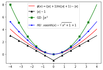
Refer to caption
(a) Regularisers
Refer to caption
(b) Mirror Maps
Figure 1: Comparison of Convex Regularisers

4.1 Algorithms in the Euclidean Space

To obtain an adaptive and optimistic algorithm, we define the following time varying function

ϕt:ℝd→ℝ,x↦αt∑i=1d((|xi|+β)ln(|xi|β+1)−|xi|),\phi_{t}:\mathbb{R}^{d}\to\mathbb{R},x\mapsto\alpha_{t}\sum_{i=1}^{d}((|x_{i}\rvert+\beta)\ln(\frac{|x_{i}\rvert}{\beta}+1)-|x_{i}\rvert), (2)

and apply it to the adaptive optimistic OMD (AO-OMD) given by

xt+1=arg⁡minx∈𝒦⁡⟨gt−ht+ht+1,x⟩+rt+1​(x)+ℬϕt+1​(x,xt)\begin{split}x_{t+1}&=\argmin_{x\in\mathcal{K}}\langle g_{t}-h_{t}+h_{t+1},x\rangle+r_{t+1}(x)+\mathcal{B}_{\phi_{t+1}}(x,x_{t})\end{split} (3)

for the sequence of subgradients {gt}\{g_{t}\} and hints {ht}\{h_{t}\}. In a bounded domain, ϕt\phi_{t} is strongly convex with respect to ∥⋅∥1\lVert\cdot\rVert_{1}, which is shown in the next lemma.

Lemma 2.

Let 𝒦⊆ℝd\mathcal{K}\subseteq\mathbb{R}^{d} be convex and bounded such that ∥x∥1≤D\lVert x\rVert_{1}\leq D for all x∈𝒦x\in\mathcal{K}. Then we have for all x,y∈𝒦x,y\in\mathcal{K}

ϕt​(x)−ϕt​(y)≥▽​ϕt​(y)⊤​(x−y)+αtD+d​β​∥x−y∥12.\phi_{t}(x)-\phi_{t}(y)\geq\triangledown\phi_{t}(y)^{\top}(x-y)+\frac{\alpha_{t}}{D+d\beta}\lVert x-y\rVert_{1}^{2}.

With the property of the strong convexity, the regret of AO-OMD with regulariser (2) can be analysed in the framework of optimistic algorithm (Joulani \BOthers. \APACyear2017) and is upper bounded by the following theorem.

Theorem 1.

Let 𝒦⊆ℝd\mathcal{K}\subseteq\mathbb{R}^{d} be a compact convex set. Assume that there is some D>0D>0 such that ∥x∥1≤D\lVert x\rVert_{1}\leq D holds for all x∈𝒦x\in\mathcal{K}. Let {xt}\{x_{t}\} be the sequence generated by update rule (3) with regulariser (2). Setting β=1d\beta=\frac{1}{d}, η=1ln⁡(D+1)+ln⁡d\eta=\sqrt{\frac{1}{\ln(D+1)+\ln d}}, and αt=η​∑s=1t−1∥gs−hs∥∞2\alpha_{t}=\eta\sqrt{\sum_{s=1}^{t-1}\lVert g_{s}-h_{s}\rVert^{2}_{\infty}}, we obtain

ℛ1:T≤r1​(x1)+c⁡(d,D)​∑t=1T∥gt−ht∥∞2\begin{split}\mathcal{R}_{1:T}\leq&r_{1}(x_{1})+c(d,D)\sqrt{\sum_{t=1}^{T}\lVert g_{t}-h_{t}\rVert_{\infty}^{2}}\end{split}

for some c⁡(d,D)∈𝒪⁡(D​ln⁡(D+1)+ln⁡d)c(d,D)\in\mathcal{O}(D\sqrt{\ln(D+1)+\ln d}).

EG can also be considered as an instance of FTRL with a constant stepsize. The update rule of the adaptive optimistic FTRL (AO-FTRL) is given by

xt+1=arg⁡minx∈𝒦⟨g1:t+ht+1,x⟩+r1:t+1(x)+ℬϕt+1(x,x1).\begin{split}x_{t+1}&=\argmin_{x\in\mathcal{K}}\langle g_{1:t}+h_{t+1},x\rangle+r_{1:t+1}(x)+\mathcal{B}_{\phi_{t+1}}(x,x_{1}).\end{split} (4)

The regret of AO-FTRL is upper bounded by the following theorem.

Theorem 2.

Let 𝒦⊆ℝd\mathcal{K}\subseteq\mathbb{R}^{d} be a compact convex set with d>ed>e. Assume that there is some D≥1D\geq 1 such that ∥x∥1≤D\lVert x\rVert_{1}\leq D holds for all x∈𝒦⊆ℝdx\in\mathcal{K}\subseteq\mathbb{R}^{d}. Let {xt}\{x_{t}\} be the sequence generated by updating rule (4) with regulariser (2) at iteration tt. Setting β=1d\beta=\frac{1}{d}, η=1ln⁡(D+1)+ln⁡d\eta=\sqrt{\frac{1}{\ln(D+1)+\ln d}} and αt=η​∑s=1t−1∥gs−hs∥∞2\alpha_{t}=\eta\sqrt{\sum_{s=1}^{t-1}\lVert g_{s}-h_{s}\rVert_{\infty}^{2}}, we obtain

ℛ1:T≤c⁡(d,D)​∑t=1T∥gt−ht∥∞2\begin{split}\mathcal{R}_{1:T}\leq&c(d,D)\sqrt{\sum_{t=1}^{T}\lVert g_{t}-h_{t}\rVert_{\infty}^{2}}\\ \end{split}

for some c⁡(d,D)∈𝒪⁡(D​ln⁡(D+1)+ln⁡d)c(d,D)\in\mathcal{O}(D\sqrt{\ln(D+1)+\ln d}).

4.2 Spectral Algorithms

We now consider the setting in which the decision variables are matrices taken from a compact convex set 𝒦⊆ℝm,n\mathcal{K}\subseteq\mathbb{R}^{m,n}. A direct attempt to solve this problem is to apply the updating rule (3) or (4) to the vectorised matrices. A regret bound of 𝒪⁡(D​T​ln⁡(m​n))\mathcal{O}(D\sqrt{T\ln(mn)}) can be guaranteed if the ℓ1\ell_{1} norm of the vectorised matrices from 𝒦\mathcal{K} are bounded by DD, which is not optimal. In many applications, elements in 𝒦\mathcal{K} are assumed to have bounded nuclear norm, for which the regulariser

Φt=ϕt∘σ\Phi_{t}=\phi_{t}\circ\sigma (5)

can be applied. The next theorem gives the strong convexity of Φt\Phi_{t} with respect to ∥⋅∥1\lVert\cdot\rVert_{1} over 𝒦\mathcal{K}, which allows us to use {Φt}\{\Phi_{t}\} as the potential functions in OMD and FTRL.

Theorem 3.

Let σ:ℝm,n→ℝd\sigma:\mathbb{R}^{m,n}\to\mathbb{R}^{d} be the function mapping a matrix to its singular values. Then the function Φt=ϕt∘σ\Phi_{t}=\phi_{t}\circ\sigma is αt2​(D+min⁡{m,n}​β)\frac{\alpha_{t}}{2(D+\min\{m,n\}\beta)}-strongly convex with respect to the nuclear norm over the nuclear ball with radius DD.

The proof of Theorem 3 follows the idea introduced in Ghai \BOthers. \APACyear2020. Define the operator

S:ℝm,n→𝕊m+n,X↦[0XX⊤0]S:\mathbb{R}^{m,n}\to\mathbb{S}^{m+n},X\mapsto\begin{bmatrix}0&X\\ X^{\top}&0\end{bmatrix}

The set 𝒳={S(X)|∈ℝm,n}\mathcal{X}=\{S(X)\lvert\in\mathbb{R}^{m,n}\} is a finite dimensional linear subspace of the space of symmetric matrices 𝕊m+n\mathbb{S}^{m+n}. Its dual space 𝒳∗\mathcal{X}_{*} determined by the Frobenius inner product can be represented by 𝒳\mathcal{X} itself. For any S⁡(X)∈𝒳S(X)\in\mathcal{X}, the set of eigenvalues of S⁡(X)S(X) consists of the singular values and the negative singular values of XX. Since ϕ\phi is even, we have ∑i=1dϕ⁡(σi​(X))=∑i=1dϕ⁡(λi​(X))\sum_{i=1}^{d}\phi(\sigma_{i}(X))=\sum_{i=1}^{d}\phi(\lambda_{i}(X)) for symmetric XX. The next lemma shows that both Φt|𝒳\Phi_{t}\lvert_{\mathcal{X}} and Φt∗|𝒳\Phi^{*}_{t}\lvert_{\mathcal{X}} are twice differentiable.

Lemma 3.

Let f:ℝ→ℝf:\mathbb{R}\to\mathbb{R} be twice continuously differentiable. Then the function given by

F:𝕊d→ℝ,X↦∑i=1df⁡(λi​(X))F:\mathbb{S}^{d}\to\mathbb{R},X\mapsto\sum_{i=1}^{d}f(\lambda_{i}(X))

is twice differentiable. Furthermore, let X∈𝕊dX\in\mathbb{S}^{d} be a symmetric matrix with eigenvalue decomposition

X=U​diag⁡(λ1​(X),…,λd​(X))​U⊤.X=U\operatorname{diag}(\lambda_{1}(X),\ldots,\lambda_{d}(X))U^{\top}.

Define the matrix of the divided difference Γ⁡(f,X)=[γ​(f,X)i​j]\Gamma(f,X)=[\gamma(f,X)_{ij}] with

γ​(f,X)i​j={f⁡(λi​(X))−f⁡(λj​(X))λi​(X)−λj​(X),if ​λi​(X)≠λj​(X)f′​(λi​(X)),otherwise\gamma(f,X)_{ij}=\begin{cases}\frac{f(\lambda_{i}(X))-f(\lambda_{j}(X))}{\lambda_{i}(X)-\lambda_{j}(X)},&\text{if }\lambda_{i}(X)\neq\lambda_{j}(X)\\ f^{\prime}(\lambda_{i}(X)),&\text{otherwise}\end{cases}

Then for any G,H∈𝕊dG,H\in\mathbb{S}^{d}, we have

D2​F​(X)​(G,H)=∑i.jγ​(f′,X)i​j​g~i​j​h~i​j,D^{2}F(X)(G,H)=\sum_{i.j}\gamma(f^{\prime},X)_{ij}\tilde{g}_{ij}\tilde{h}_{ij},\\

where g~i​j\tilde{g}_{ij} and h~i​j\tilde{h}_{ij} are the elements of the ii-th row and jj-th column of the matrix U⊤​G​UU^{\top}GU and U⊤​H​UU^{\top}HU, respectively.

Lemma 3 implies the unsurprising positive semidefiniteness of D2​F​(X)D^{2}F(X) for convex ff. Furthermore, the exact expression of the second differential allows us to show the local smoothness of Φt∗\Phi^{*}_{t} using the local smoothness of ϕ∗\phi^{*}. Together with Lemma 4, the locally strong convexity of Φt|𝒳\Phi_{t}\lvert_{\mathcal{X}} can be proved.

Lemma 4.

Let Φ:𝕏→ℝ\Phi:\mathbb{X}\to\mathbb{R} be a closed convex function such that Φ∗\Phi^{*} is twice differentiable at some θ∈𝕏∗\theta\in\mathbb{X}_{*} with positive definite D2​Φ∗​(θ)∈ℒ⁡(𝕏∗,ℒ⁡(𝕏∗,ℝ))D^{2}\Phi^{*}(\theta)\in\mathcal{L}(\mathbb{X}_{*},\mathcal{L}(\mathbb{X}_{*},\mathbb{R})). Suppose that D2​Φ∗​(θ)​(v,v)≤∥v∥∗2D^{2}\Phi^{*}(\theta)(v,v)\leq\lVert v\rVert_{*}^{2} holds for all v∈𝕏∗v\in\mathbb{X}_{*}. Then we have D2​Φ​(D​Φ∗​(θ))​(x,x)≥∥x∥2D^{2}\Phi(D\Phi^{*}(\theta))(x,x)\geq\lVert x\rVert^{2} for all x∈𝕏x\in\mathbb{X}.

Lemma 4 can be considered as a generalised version of the local duality of smoothness and convexity proved in Ghai \BOthers. \APACyear2020. The required positive definiteness of D2​Φt∗​(θ)D^{2}\Phi^{*}_{t}(\theta) is guaranteed by the exact expression of the second differential described in Lemma 3 and the fact ϕ∗′′(θ)>0\phi^{*\prime\prime}(\theta)>0 for all θ∈ℝ\theta\in\mathbb{R}. Finally, using the construction of 𝒳\mathcal{X}, the locally strong convexity of Φt|𝒳\Phi_{t}\lvert_{\mathcal{X}} can be extended to Φt\Phi_{t}. The complete proofs of Theorem 3 and the technical lemmata can be found in Appendix 9.1.

With the property of the strong convexity, the regret of applying (5) to AO-OMD and AO-FTRL can be upper bounded by the following theorems.

Theorem 4.

Let 𝒦⊆ℝm,n\mathcal{K}\subseteq\mathbb{R}^{m,n} be a compact convex set. Assume that there is some D>0D>0 such that ∥x∥1≤D\lVert x\rVert_{1}\leq D holds for all x∈𝒦x\in\mathcal{K}. Let {xt}\{x_{t}\} be the sequence generated by update rule (3) with regulariser (5) at iteration tt. Setting β=1min⁡{m,n}\beta=\frac{1}{\min\{m,n\}}, η=1ln⁡(D+1)+ln⁡min⁡{m,n}\eta=\sqrt{\frac{1}{\ln(D+1)+\ln\min\{m,n\}}}, and αt=η​∑s=1t−1∥gs−hs∥∞2\alpha_{t}=\eta\sqrt{\sum_{s=1}^{t-1}\lVert g_{s}-h_{s}\rVert^{2}_{\infty}}, we obtain

ℛ1:T≤r1​(x1)+c⁡(m,n,D)​∑t=1T∥gt−ht∥∞2\begin{split}\mathcal{R}_{1:T}\leq&r_{1}(x_{1})+c(m,n,D)\sqrt{\sum_{t=1}^{T}\lVert g_{t}-h_{t}\rVert_{\infty}^{2}}\end{split}

with c⁡(m,n,D)∈𝒪⁡(D​ln⁡(D+1)+ln⁡min⁡{m,n})c(m,n,D)\in\mathcal{O}(D\sqrt{\ln(D+1)+\ln\min\{m,n\}}).

Theorem 5.

Let 𝒦⊆ℝmin⁡{m,n}\mathcal{K}\subseteq\mathbb{R}^{\min\{m,n\}} be a compact convex set with min⁡{m,n}>e\min\{m,n\}>e. Assume that there is some D≥1D\geq 1 such that ∥x∥1≤D\lVert x\rVert_{1}\leq D holds for all x∈𝒦x\in\mathcal{K}. Let {xt}\{x_{t}\} be the sequence generated by updating rule (4) with time varying regulariser (5). Setting β=1min⁡{m,n}\beta=\frac{1}{\min\{m,n\}}, η=1ln⁡(D+1)+ln⁡min⁡{m,n}\eta=\sqrt{\frac{1}{\ln(D+1)+\ln\min\{m,n\}}} and αt=η​∑s=1t−1∥gs−hs∥∞2\alpha_{t}=\eta\sqrt{\sum_{s=1}^{t-1}\lVert g_{s}-h_{s}\rVert_{\infty}^{2}}, we obtain

ℛ1:T≤c⁡(m,n,D)​∑t=1T∥gt−ht∥∞2,\begin{split}\mathcal{R}_{1:T}\leq&c(m,n,D)\sqrt{\sum_{t=1}^{T}\lVert g_{t}-h_{t}\rVert_{\infty}^{2}},\\ \end{split}

with c⁡(m,n,D)∈𝒪⁡(D​ln⁡(D+1)+ln⁡min⁡{m,n})c(m,n,D)\in\mathcal{O}(D\sqrt{\ln(D+1)+\ln\min\{m,n\}}).

With regulariser (5), both AO-OMD and AO-FTRL guarantee a regret upper bound proportional to ln⁡min​{m,n}\sqrt{\ln\min\{m,n\}}, which is the best known dependence on the size of the matrices.

5 Derived Algorithms

Given zt+1∈𝕏∗z_{t+1}\in\mathbb{X}_{*} and a time varying closed convex function Rt+1:𝒦→ℝR_{t+1}:\mathcal{K}\to\mathbb{R}, we consider the following updating rule

yt+1=▽​ϕt+1∗​(zt+1)xt+1=arg⁡minx∈𝒦⁡Rt+1​(x)+ℬϕt+1​(x,yt+1).\begin{split}y_{t+1}&=\triangledown\phi^{*}_{t+1}(z_{t+1})\\ x_{t+1}&=\argmin_{x\in\mathcal{K}}R_{t+1}(x)+\mathcal{B}_{\phi_{t+1}}(x,y_{t+1}).\end{split} (6)

It is easy to verify that (6) is equivalent to

xt+1=arg⁡minx∈𝒦⁡Rt+1​(x)+ℬϕt+1​(x,yt+1)=arg⁡minx∈𝒦⁡Rt+1​(x)+ϕt+1​(x)−⟨▽​ϕt+1​(yt+1),x⟩=arg⁡minx∈𝒦⁡Rt+1​(x)+ϕt+1​(x)−⟨zt+1,x⟩\begin{split}x_{t+1}=&\argmin_{x\in\mathcal{K}}R_{t+1}(x)+\mathcal{B}_{\phi_{t+1}}(x,y_{t+1})\\ =&\argmin_{x\in\mathcal{K}}R_{t+1}(x)+\phi_{t+1}(x)-\langle\triangledown\phi_{t+1}(y_{t+1}),x\rangle\\ =&\argmin_{x\in\mathcal{K}}R_{t+1}(x)+\phi_{t+1}(x)-\langle z_{t+1},x\rangle\\ \end{split}

Setting zt+1=▽​ϕt+1​(xt)−gt+ht−ht+1z_{t+1}=\triangledown\phi_{t+1}(x_{t})-g_{t}+h_{t}-h_{t+1} and Rt+1=rt+1R_{t+1}=r_{t+1}, we obtain the AO-OMD update

xt+1=arg⁡minx∈𝒦⁡⟨gt−ht+ht+1,x⟩−⟨▽​ϕt+1​(xt),x⟩+ϕt+1​(x)+rt+1​(x)=arg⁡minx∈𝒦⁡⟨gt−ht+ht+1,x⟩+rt+1​(x)+ℬϕt+1​(x,xt).\begin{split}x_{t+1}=&\argmin_{x\in\mathcal{K}}\langle g_{t}-h_{t}+h_{t+1},x\rangle-\langle\triangledown\phi_{t+1}(x_{t}),x\rangle+\phi_{t+1}(x)+r_{t+1}(x)\\ =&\argmin_{x\in\mathcal{K}}\langle g_{t}-h_{t}+h_{t+1},x\rangle+r_{t+1}(x)+\mathcal{B}_{\phi_{t+1}}(x,x_{t}).\\ \end{split}

Setting zt+1=−▽ϕt+1(x1)+g1:t+ht+1z_{t+1}=-\triangledown\phi_{t+1}(x_{1})+g_{1:t}+h_{t+1} and Rt+1=r1:t+1R_{t+1}=r_{1:t+1}, we obtain the AO-FTRL update

xt+1=arg⁡minx∈𝒦⟨g1:t−θ1+ht+1,x⟩+ϕt+1(x)+r1:t+1(x).\begin{split}x_{t+1}=&\argmin_{x\in\mathcal{K}}\langle g_{1:t}-\theta_{1}+h_{t+1},x\rangle+\phi_{t+1}(x)+r_{1:t+1}(x).\\ \end{split}

The rest of this section focuses on solving the second line of (6) for some popular choices of rr and 𝒦\mathcal{K}.

5.1 Elastic Net Regularisation

We first consider the setting of 𝒦=ℝd\mathcal{K}=\mathbb{R}^{d} and Rt+1​(x)=γ1​∥x∥1+γ22​∥x∥22R_{t+1}(x)=\gamma_{1}\lVert x\rVert_{1}+\frac{\gamma_{2}}{2}\lVert x\rVert^{2}_{2}, which has countless applications in machine learning. It is easy to verify that the Bregman divergence associated with ψt+1\psi_{t+1} is given by

ℬϕt+1​(x,y)=αt+1∑i=1d((|xi|+β)ln(|xi|β+1)−|xi|−(sgn(yi)xi+β)ln(|yi|β+1)+|yi|).\begin{split}\mathcal{B}_{\phi_{t+1}}(x,y)=&\alpha_{t+1}\sum_{i=1}^{d}((|x_{i}\rvert+\beta)\ln(\frac{|x_{i}\rvert}{\beta}+1)-|x_{i}\rvert\\ &-(\operatorname{sgn}(y_{i})x_{i}+\beta)\ln(\frac{|y_{i}\rvert}{\beta}+1)+|y_{i}\rvert).\end{split}

The minimiser of

Rt+1​(x)+ℬϕt+1​(x,yt+1)R_{t+1}(x)+\mathcal{B}_{\phi_{t+1}}(x,y_{t+1})

in ℝd\mathbb{R}^{d} can be simply obtained by setting the subgradient to 00. For ln⁡(|yi,t+1|β+1)≤γ1αt+1\ln(\frac{|y_{i,t+1}\rvert}{\beta}+1)\leq\frac{\gamma_{1}}{\alpha_{t+1}}, we set xi,t+1=0x_{i,t+1}=0. Otherwise, the 00 subgradient implies sgn⁡(xi,t+1)=sgn⁡(yi,t+1)\operatorname{sgn}(x_{i,t+1})=\operatorname{sgn}(y_{i,t+1}) and |xi,t+1||x_{i,t+1}\rvert given by the root of

ln(|yi,t+1|β+1)=ln(|xi,t+1|β+1)+γ1αt+1+γ2αt+1|xi,t+1|\begin{split}\ln(\frac{|y_{i,t+1}\rvert}{\beta}+1)=\ln(\frac{|x_{i,t+1}\rvert}{\beta}+1)+\frac{\gamma_{1}}{\alpha_{t+1}}+\frac{\gamma_{2}}{\alpha_{t+1}}|x_{i,t+1}\rvert\end{split}

for i=1,…,di=1,\ldots,d. For simplicity, we set a=βa=\beta, b=γ2αt+1b=\frac{\gamma_{2}}{\alpha_{t+1}} and c=γ1αt+1−ln⁡(|yi,t+1|β+1)c=\frac{\gamma_{1}}{\alpha_{t+1}}-\ln(\frac{|y_{i,t+1}\rvert}{\beta}+1). It can be verified that |xi,t+1||x_{i,t+1}\rvert is given by

|xi,t+1|=1bW0(abexp(ab−c))−a,|x_{i,t+1}\rvert=\frac{1}{b}W_{0}(ab\exp(ab-c))-a, (7)

where W0W_{0} is the principal branch of the Lambert function and can be well approximated. For γ2=0\gamma_{2}=0, i.e. the ℓ1\ell_{1} regularised problem, |xi,t+1||x_{i,t+1}\rvert has the closed form solution

|xi,t+1|=βexp(ln(|yi,t+1|β+1)−γ1αt+1)−β.|x_{i,t+1}\rvert=\beta\exp(\ln(\frac{|y_{i,t+1}\rvert}{\beta}+1)-\frac{\gamma_{1}}{\alpha_{t+1}})-\beta. (8)

The implementation is described in Algorithm 1.

Algorithm 1 Solving minx∈ℝd⁡Rt+1​(x)+ℬϕt+1​(x,yt+1)\min_{x\in\mathbb{R}^{d}}R_{t+1}(x)+\mathcal{B}_{\phi_{t+1}}(x,y_{t+1})
for i=1,…,di=1,\ldots,d do
  if ln⁡(|yi,t+1|β+1)≤γ1αt+1\ln(\frac{|y_{i,t+1}\rvert}{\beta}+1)\leq\frac{\gamma_{1}}{\alpha_{t+1}} then
   xt+1,i←0x_{t+1,i}\leftarrow 0
  else
   a←βa\leftarrow\beta
   b←γ2αt+1b\leftarrow\frac{\gamma_{2}}{\alpha_{t+1}}
   c←γ1αt+1−ln⁡(|yt+1,i|β+1)c\leftarrow\frac{\gamma_{1}}{\alpha_{t+1}}-\ln(\frac{|{y}_{t+1,i}\rvert}{\beta}+1)
   xt+1,i←1b​W0​(a​b​exp⁡(a​b−c))−ax_{t+1,i}\leftarrow\frac{1}{b}W_{0}(ab\exp(ab-c))-a
  end if
end for
Return xt+1x_{t+1}

5.2 Nuclear and Frobenius Regularisation

Similarly, we consider 𝒦=ℝm,n\mathcal{K}=\mathbb{R}^{m,n} with a regulariser Rt+1​(x)=γ1​∥x∥1+γ22​∥x∥22R_{t+1}(x)=\gamma_{1}\lVert x\rVert_{1}+\frac{\gamma_{2}}{2}\lVert x\rVert^{2}_{2} mixed with the nuclear and Frobenius norm. The second line of update rule (6) can be implemented as follows

Compute SVD: yt+1=Ut+1​diag⁡(y~t+1)​Vt+1⊤Apply Algorithm 1: x~t+1=arg⁡minx∈ℝd⁡Rt+1​(x)+ℬϕt+1​(x,y~t+1)Construct: xt+1=Ut+1​diag⁡(x~t+1)​Vt+1⊤.\begin{split}\text{Compute SVD: }y_{t+1}=&U_{t+1}\operatorname{diag}(\tilde{y}_{t+1})V_{t+1}^{\top}\\ \text{Apply Algorithm~\ref{alg:reg}: }\tilde{x}_{t+1}=&\argmin_{x\in\mathbb{R}^{d}}R_{t+1}(x)+\mathcal{B}_{\phi_{t+1}}(x,\tilde{y}_{t+1})\\ \text{Construct: }x_{t+1}=&U_{t+1}\operatorname{diag}(\tilde{x}_{t+1})V_{t+1}^{\top}.\end{split} (9)

Let yt+1y_{t+1} and y~t+1\tilde{y}_{t+1} be as defined in (9). It is easy to verify

arg⁡minx∈ℝm,n⁡Rt+1​(x)+ℬΦt+1​(x,yt+1)=arg⁡minx∈ℝm,n⁡Rt+1​(x)+Φt+1​(x)−⟨Ut+1​diag⁡(▽​ϕt+1​(y~t+1))​Vt+1⊤,x⟩F.\begin{split}&\argmin_{x\in\mathbb{R}^{m,n}}R_{t+1}(x)+\mathcal{B}_{\Phi_{t+1}}(x,y_{t+1})\\ =&\argmin_{x\in\mathbb{R}^{m,n}}R_{t+1}(x)+\Phi_{t+1}(x)-\langle U_{t+1}\operatorname{diag}(\triangledown\phi_{t+1}(\tilde{y}_{t+1}))V_{t+1}^{\top},x\rangle_{F}.\end{split} (10)

From the characterisation of subgradient, it follows

▽​Rt+1​(x)=U​diag⁡(γ1​sgn⁡(σ⁡(x))+γ2​σ​(x))​V⊤,\begin{split}\triangledown R_{t+1}(x)=U\operatorname{diag}(\gamma_{1}\operatorname{sgn}(\sigma(x))+\gamma_{2}\sigma(x))V^{\top},\end{split}

and

▽​Φt​(x)=U​diag⁡(▽​ϕt​(σ⁡(x)))​V⊤,\begin{split}\triangledown\Phi_{t}(x)=U\operatorname{diag}(\triangledown\phi_{t}(\sigma(x)))V^{\top},\end{split}

where x=U​diag⁡(σ⁡(x))​V⊤x=U\operatorname{diag}(\sigma(x))V^{\top} is SVD of xx. Similar to the case in ℝd\mathbb{R}^{d}, x~t+1\tilde{x}_{t+1} is the root of

γ1​sgn⁡(σ⁡(x))+γ2​σ​(x)+▽​ϕt​(σ⁡(x))=▽​ϕt​(y~t+1).\gamma_{1}\operatorname{sgn}(\sigma(x))+\gamma_{2}\sigma(x)+\triangledown\phi_{t}(\sigma(x))=\triangledown\phi_{t}(\tilde{y}_{t+1}).

The subgradient of the objective (10) at xt+1=Ut+1​diag⁡(x~t+1)​Vt+1⊤x_{t+1}=U_{t+1}\operatorname{diag}(\tilde{x}_{t+1})V_{t+1}^{\top} is clearly 00.

5.3 Projection onto the Cross-Polytope

Next, we consider the setting where rtr_{t} is the zero function and 𝒦\mathcal{K} is the ℓ1\ell_{1} ball with radius DD. Clearly, we simply set xt+1=yt+1x_{t+1}=y_{t+1} for ∥yt+1∥1≤D\lVert y_{t+1}\rVert_{1}\leq D. Otherwise, Algorithm 2 describes a sorting based procedure projecting yt+1y_{t+1} onto the ℓ1\ell_{1} ball with time complexity 𝒪⁡(d​log⁡d)\mathcal{O}(d\log d). The correctness of the algorithm is shown in the next lemma.

Algorithm 2 project⁡(y,D,β)\operatorname{project}(y,D,\beta)
Sort |yi||y_{i}\rvert to get the permutation pp such that |yp⁡(i)|≤|yp⁡(i+1)||y_{p(i)}\rvert\leq|y_{p(i+1)}\rvert
Define θ(j)=|yp⁡(j)|(D+(d−j+1)β)+βD−β∑i≥j|yp⁡(i)|\theta(j)=|y_{p(j)}\rvert(D+(d-j+1)\beta)+\beta D-\beta\sum_{i\geq j}|y_{p(i)}\rvert
ρ←min{j|θ(j)>0}\rho\leftarrow\min\{j\lvert\theta(j)>0\}
z←∑i=ρd(|yp⁡(i)|+β)D+(d−ρ+1)​βz\leftarrow\frac{\sum_{i=\rho}^{d}(|y_{p(i)}\rvert+\beta)}{D+(d-\rho+1)\beta}
xi∗←max⁡{|yi|+βz−β,0}​sgn⁡(yi)x^{*}_{i}\leftarrow\max\{\frac{|y_{i}\rvert+\beta}{z}-\beta,0\}\operatorname{sgn}(y_{i}) for i=1​…​di=1\ldots d
Return x∗x^{*} 
Lemma 5.

Let y∈ℝdy\in\mathbb{R}^{d} with ∥y∥1>D\lVert y\rVert_{1}>D and x∗x^{*} as returned by Algorithm 2, then we have

x∗∈arg⁡minx∈𝒦⁡ℬψt+1​(x,y).x^{*}\in\argmin_{x\in\mathcal{K}}\mathcal{B}_{\psi_{t+1}}(x,y).

For the case that 𝒦⊆ℝm,n\mathcal{K}\subseteq\mathbb{R}^{m,n} is the nuclear ball with radius DD and ∥yt+1∥1>D\lVert y_{t+1}\rVert_{1}>D, we need to solve the problem

minx∈𝒦⁡Φt+1​(x)−⟨Ut+1​diag⁡(▽​ϕt+1​(y~t+1))​Vt+1⊤,x⟩F,\min_{x\in\mathcal{K}}\Phi_{t+1}(x)-\langle U_{t+1}\operatorname{diag}(\triangledown\phi_{t+1}(\tilde{y}_{t+1}))V_{t+1}^{\top},x\rangle_{F},

where the constant part of the Bregman divergence is removed. From the von Neumann’s trace inequality, the Frobenius inner product is upper bounded by

⟨Ut+1​▽​ϕt+1​(y~t+1)​Vt+1⊤,x⟩F≤σ​(x)⊤​▽​ϕt+1​(y~t+1).\langle U_{t+1}\triangledown\phi_{t+1}(\tilde{y}_{t+1})V_{t+1}^{\top},x\rangle_{F}\leq\sigma(x)^{\top}\triangledown\phi_{t+1}(\tilde{y}_{t+1}).

The equality holds when xx and Ut+1​▽​ϕt+1​(y~t+1)​Vt+1⊤U_{t+1}\triangledown\phi_{t+1}(\tilde{y}_{t+1})V_{t+1}^{\top} share a simultaneous SVD, i.e. the minimiser has an SVD of the form

x=Ut+1​diag⁡(▽​σ​(x))​Vt+1⊤.x=U_{t+1}\operatorname{diag}(\triangledown\sigma(x))V_{t+1}^{\top}.

Thus the problem is reduced to

minx∈ℝmin⁡{m,n}ϕt+1​(x)−▽​ϕt+1​(y~t+1)⊤​xs.t.∑i=1min⁡{m,n}xi≤Dxi≥0​ for all ​i=1,…,min⁡{m,n},\begin{split}\min_{x\in\mathbb{R}^{\min\{m,n\}}}&\phi_{t+1}(x)-\triangledown\phi_{t+1}(\tilde{y}_{t+1})^{\top}x\\ \textrm{s.t.}\quad&\sum_{i=1}^{\min\{m,n\}}x_{i}\leq D\\ &x_{i}\geq 0\textrm{ for all }i=1,\ldots,\min\{m,n\},\\ \end{split}

which can be solved by Algorithm 2. Thus, the projection of update rule (6) can be implemented as follows

Compute SVD: yt+1=Ut+1​diag⁡(y~t+1)​Vt+1⊤Apply Algorithm 2: x~t+1=project⁡(y~t+1,D,β)Construct: xt+1=Ut+1​diag⁡(x~t+1)​Vt+1⊤.\begin{split}\text{Compute SVD: }y_{t+1}=&U_{t+1}\operatorname{diag}(\tilde{y}_{t+1})V_{t+1}^{\top}\\ \text{Apply Algorithm~\ref{ALG:Proj}: }\tilde{x}_{t+1}=&\operatorname{project}(\tilde{y}_{t+1},D,\beta)\\ \text{Construct: }x_{t+1}=&U_{t+1}\operatorname{diag}(\tilde{x}_{t+1})V_{t+1}^{\top}.\end{split} (11)

5.4 Stochastic Acceleration

Finally, we consider the stochastic optimisation problem of the form

minx∈𝒦⁡l⁡(x)+r⁡(x),\min_{x\in\mathcal{K}}l(x)+r(x),

where l:𝕏→ℝl:\mathbb{X}\to\mathbb{R} and r:𝒦→ℝ≥0r:\mathcal{K}\to\mathbb{R}_{\geq 0} are closed convex functions. In the stochastic setting, instead of having a direct access to ▽​l\triangledown l, we query a stochastic gradient gtg_{t} of ll at ztz_{t} in each iteration tt with 𝔼[gt|zt]∈∂l(zt)\mathbb{E}[g_{t}\lvert z_{t}]\in\partial l(z_{t}). Algorithms with a regret bound of the form 𝒪⁡(∑t=1T∥gt−ht∥∗2)\mathcal{O}(\sqrt{\sum_{t=1}^{T}\lVert g_{t}-h_{t}\rVert_{*}^{2}}) can be easily converted into a stochastic optimisation algorithm by applying the update rule to the scaled stochastic gradient at​gta_{t}g_{t} and hint at+1​gta_{t+1}g_{t}, which is described in Algorithm 3.

Algorithm 3 Stochastic Acceleration
Input: optimistic algorithm 𝒜\mathcal{A}, compact convex set 𝒦\mathcal{K} and closed convex function rr 
for t=1,…,Tt=1,\ldots,T do
  at←ta_{t}\leftarrow t
  xtx_{t} from 𝒜\mathcal{A}
  zt←ata1:txt+(1−ata1:t)zt−1z_{t}\leftarrow\frac{a_{t}}{a_{1:t}}x_{t}+(1-\frac{a_{t}}{a_{1:t}})z_{t-1}
  Query gtg_{t} such that 𝔼[gt|zt]∈∂l(zt)\mathbb{E}[g_{t}\lvert z_{t}]\in\partial l(z_{t})
  Update 𝒜\mathcal{A} with 𝒦\mathcal{K}, αt+1​r\alpha_{t+1}r, scaled subgradient at​gta_{t}g_{t} and hint at+1​gta_{t+1}g_{t}
end for
Return xt+1x_{t+1}

Joulani \BOthers. \APACyear2020 has shown the convergence of accelerating Adagrad for the problem in ℝd\mathbb{R}^{d}. We extend the result to any finite dimensional normed vector space in the following corollary.

Corollary 1.

Let (𝕏,∥⋅∥)(\mathbb{X},\lVert\cdot\rVert) be a finite dimensional normed vector space and 𝒦⊆𝕏\mathcal{K}\subseteq\mathbb{X} a compact convex set. Denote by 𝒜\mathcal{A} be some optimistic algorithm generating xt∈𝒦x_{t}\in\mathcal{K} at iteration tt. Denote by

νt2=𝔼[∥gt−▽lt(zt)∥∗2|zt]\nu_{t}^{2}=\mathbb{E}[\lVert g_{t}-\triangledown l_{t}(z_{t})\rVert_{*}^{2}\lvert z_{t}]

the variance. If 𝒜\mathcal{A} has a regret upper bound in the form of

c1+c2​∑t=1T∥at​(gt−gt−1)∥∗2c_{1}+c_{2}\sqrt{\sum_{t=1}^{T}\lVert a_{t}(g_{t}-g_{t-1})\rVert_{*}^{2}}

then there is some L>0L>0 such that the error incurred by Algorithm 3 is upper bounded by

𝔼⁡[f⁡(zT)−f⁡(x)]≤c1+c2​8​∑t=1Tat2​(νt2+L2)a1:T.\begin{split}\mathbb{E}[f(z_{T})-f(x)]\leq&\frac{c_{1}+c_{2}\sqrt{8\sum_{t=1}^{T}a_{t}^{2}(\nu_{t}^{2}+L^{2})}}{a_{1:T}}.\\ \end{split}

Furthermore, if ll is MM-smooth, then we have

𝔼⁡[f⁡(zT)−f⁡(x)]≤c1+c2​8​∑t=1Tat2​νt2+2​c2​L+2​M​c22a1:T.\begin{split}\mathbb{E}[f(z_{T})-f(x)]\leq&\frac{c_{1}+c_{2}\sqrt{8\sum_{t=1}^{T}a_{t}^{2}\nu_{t}^{2}}+\sqrt{2}c_{2}L+2Mc_{2}^{2}}{a_{1:T}}.\\ \end{split}

Setting αt=t\alpha_{t}=t, we obtain a convergence of 𝒪⁡(c2T)\mathcal{O}(\frac{c_{2}}{\sqrt{T}}) in general case, and 𝒪⁡(c2T2+c2​maxt​νtT)\mathcal{O}(\frac{c_{2}}{T^{2}}+\frac{c_{2}\max_{t}\nu_{t}}{\sqrt{T}}) for smooth loss function. Applying update rule (3) or (4) with regulariser (2) or (5) to Algorithm 3, the constant c2c_{2} is proportional to ln⁡d\sqrt{\ln d} and ln⁡(min⁡{m,n})\sqrt{\ln(\min\{m,n\})} for 𝕏=ℝd\mathbb{X}=\mathbb{R}^{d} and 𝕏=ℝm,n\mathbb{X}=\mathbb{R}^{m,n} respectively, while the accelerated AdaGrad has a linear dependence on the dimensionality (Joulani \BOthers. \APACyear2020).

6 Experiments

This section shows the empirical evaluation of the developed algorithms. We carry out experiments on both synthetic and real-world data and demonstrate the performances of the OMD (Exp-MD) and FTRL (Exp-FTRL) based on the exponentiated update.

6.1 Online Logistic Regression

For a sanity check, we simulate an dd-dimensional online logistic regression problem, in which the model parameter w∗w^{*} has a 99%99\% sparsity and the non-zero values are randomly drawn from the uniform distribution over [−1,1][-1,1]. At each iteration tt, we sample a random feature vector xtx_{t} from a uniform distribution over [−1,1]d[-1,1]^{d} and generate a label yt∈{−1,1}y_{t}\in\{-1,1\} using a logit model, i.e. Pr[yt=1]=(1+exp(−w⊤xt))−1\operatorname{Pr}[y_{t}=1]=(1+\exp(-w^{\top}x_{t}))^{-1}. The goal is to minimise the cumulative regret

ℛ1:T=∑t=1Tlt(wt)−∑t=1Tlt(w∗)\mathcal{R}_{1:T}=\sum_{t=1}^{T}l_{t}(w_{t})-\sum_{t=1}^{T}l_{t}(w^{*})

with lt​(w)=ln⁡(1+exp⁡(−yt​w⊤​xt))l_{t}(w)=\ln(1+\exp(-y_{t}w^{\top}x_{t})). We choose d=10,000d=10,000 and compare our algorithms with AdaGrad, AdaFTRL (J. Duchi \BOthers. \APACyear2011) and HU (Ghai \BOthers. \APACyear2020). For both AdaGrad and AdaFTRL, we set the ii-th entry of the proximal matrix HtH_{t} to hi​i=10−6+∑s=1t−1gs,i2h_{ii}=10^{-6}+\sum_{s=1}^{t-1}g_{s,i}^{2} as their theory suggested (J. Duchi \BOthers. \APACyear2011). The stepsize of HU is set to 1∑s=1t−1∥gs∥∞2\sqrt{\frac{1}{\sum_{s=1}^{t-1}\lVert g_{s}\rVert_{\infty}^{2}}} leading to an adaptive regret upper bound. All algorithms take decision variables from an ℓ1\ell_{1} ball {w∈ℝd|∥w∥1≤D}\{w\in\mathbb{R}^{d}\lvert\lVert w\rVert_{1}\leq D\}, which is the ideal case for HU. We examine the performances of the algorithms with known, underestimated and overestimated ∥w∗∥1\lVert w^{*}\rVert_{1} by setting D=∥w∗∥1D=\lVert w^{*}\rVert_{1}, D=12​∥w∗∥1D=\frac{1}{2}\lVert w^{*}\rVert_{1} and D=2​∥w∗∥1D=2\lVert w^{*}\rVert_{1}, respectively. For each choice of DD, we simulate the online process of each algorithm for 10,00010,000 iterations and repeat the experiments for 2020 trials.

Figure 2 plots the curves of the average cumulative regret with the ranges of standard deviation as shaded regions. As can be observed, our algorithms have a clear and stable advantage over the AdaGrad-style algorithms and slightly outperform HU in the experiments with known ∥w∗∥1\lVert w^{*}\rVert_{1}. As the combination of the entropy-like regulariser and FTRL can also be used for parameter-free optimisation (Cutkosky \BBA Boahen \APACyear2017\APACexlab\BCnt1), overestimating ∥w∗∥1\lVert w^{*}\rVert_{1} does not have a tangible impact on the performance of Exp-FTRL, which leads to its clear advantage over the rest.

Refer to caption
(a) D=∥w∗∥1\lVert w^{*}\rVert_{1}
Refer to caption
(b) D=12​∥w∗∥1D=\frac{1}{2}\lVert w^{*}\rVert_{1}
Refer to caption
(c) D=2​∥w∗∥1D=2\lVert w^{*}\rVert_{1}
Figure 2: Online Logistic Regression

6.2 Online Multitask Learning

Next, we examine the performance of the developed spectral algorithms using a simulated online multi-task learning problem (Kakade \BOthers. \APACyear2012), in which we need to solve kk highly correlated dd-dimensional online prediction problems simultaneously. The data are generated as follows. We first randomly draw two orthogonal matrices U∈GL⁡(d,ℝ)U\in\operatorname{GL}(d,\mathbb{R}) and V∈GL⁡(k,ℝ)V\in\operatorname{GL}(k,\mathbb{R}). Then we generate a kk-dimensional vector σ\sigma with rr non-zero values randomly drawn from a uniform distribution over [0,10][0,10] and construct a low rank parameter matrix W∗=U​diag⁡(σ)​VW^{*}=U\operatorname{diag}(\sigma)V. At each iteration tt, kk feature and label pairs (xt,1,yt,1),…,(xt,k,yt,k)(x_{t,1},y_{t,1}),\ldots,(x_{t,k},y_{t,k}) are generated using kk logit models with the ii-th parameters taken from the ii-th rows of WW. The loss function is given by lt​(W)=∑i=1kln⁡(1+exp⁡(−yt,i​wi⊤​xt,i))l_{t}(W)=\sum_{i=1}^{k}\ln(1+\exp(-y_{t,i}w_{i}^{\top}x_{t,i})). We set d=100d=100, k=25k=25 and r=5r=5, take the nuclear ball {W∈ℝd,k|∥W∥1≤D}\{W\in\mathbb{R}^{d,k}\lvert\lVert W\rVert_{1}\leq D\} as the decision set and run the experiment as in subsection 6.1. The average and standard deviation of the results over 2020 trials are shown in Figure 3.

Similar to the online logistic regression, our algorithms have a clear advantage over AdaGrad and AdaFTRL and slightly outperform HU in all settings. While the regret of the AdaGrad-style algorithms spread over a wider range, our algorithms yield relatively stabler results. The superiority of Exp-FTRL for the overestimated ∥W∗∥1\lVert W^{*}\rVert_{1} can also be observed from figure 3(c).

Refer to caption
(a) D=∥W∗∥1D=\lVert W^{*}\rVert_{1}
Refer to caption
(b) Underestimated D=12​∥W∗∥1D=\frac{1}{2}\lVert W^{*}\rVert_{1}
Refer to caption
(c) Overestimated D=2​∥W∗∥1D=2\lVert W^{*}\rVert_{1}
Figure 3: Online Multitask Learning

6.3 Optimisation for Contrastive Explanations

Generating the contrastive explanation of a machine learning model (Dhurandhar \BOthers. \APACyear2018) is the most motivating application of this paper. Given a sample x0∈𝒳x_{0}\in\mathcal{X} and machine learning model f:𝒳→ℝKf:\mathcal{X}\to\mathbb{R}^{K}, the contrastive explanation consists of a set of pertinent positive (PP) features and a set of pertinent negative (PN) features, which can be found by solving the following optimisation problem (Dhurandhar \BOthers. \APACyear2018)

minx∈𝒲lx0​(x)+λ1​∥x∥1+λ22​∥x∥22.\begin{split}\min_{x\in\mathcal{W}}\quad&l_{x_{0}}(x)+\lambda_{1}\lVert x\rVert_{1}+\frac{\lambda_{2}}{2}\lVert x\rVert_{2}^{2}.\\ \end{split}

Let κ≥0\kappa\geq 0 be a constant and define k0=arg⁡maxi​f​(x0)ik_{0}=\arg\max_{i}f(x_{0})_{i}. The loss function for finding PP is given by

lx0​(x)=max⁡{maxi≠k0⁡f​(x)i−f​(x)k0,−κ},l_{x_{0}}(x)=\max\{\max_{i\neq k_{0}}f(x)_{i}-f(x)_{k_{0}},-\kappa\},

which imposes a penalty on the features that do not justify the prediction. PN is the set of features altering the final classification and is modelled by the following loss function

lx0​(x)=max⁡{f​(x0+x)k0−maxi≠k0⁡f​(x0+x)i,−κ}.l_{x_{0}}(x)=\max\{f(x_{0}+x)_{k_{0}}-\max_{i\neq k_{0}}f(x_{0}+x)_{i},-\kappa\}.

In the experiment, we first train a ResNet2020 model (He \BOthers. \APACyear2016) on the CIFAR-1010 dataset (Krizhevsky \APACyear2009), which attains a test accuracy of 91.49%91.49\%. For each class of the images, we randomly pick 100100 correctly classified images from the test dataset and generate PP and PN for them. For PP, we take the set of all feasible images as the decision set, while for PN, we take the set of tensors xx, such that x0+xx_{0}+x is a feasible image.

We first consider the white-box setting, in which we have the access to ▽​lx0\triangledown l_{x_{0}}. Our goal is to demonstrate the performance of the accelerated AO-OMD and AO-FTRL based on the exponentiated update (AccAOExpMD and AccAOExpFTRL). In Dhurandhar \BOthers. \APACyear2018, the fast iterative shrinkage-thresholding algorithm (FISTA) (Beck \BBA Teboulle \APACyear2009) is applied to finding the PP and PN. Therefore, we take FISTA as our baseline. In addition, our algorithms are also compared with the accelerated AO-OMD and AO-FTRL with AdaGrad-style stepsizes (AccAOMD and AccAOFTRL) (Joulani \BOthers. \APACyear2020).

We pick λ1=λ2=12\lambda_{1}=\lambda_{2}=\frac{1}{2}, which is the largest value from the set {2−i|i∈ℕ}\{2^{-i}\lvert i\in\mathbb{N}\} allowing FISTA to attain a negative loss lx0l_{x_{0}} for 1010 randomly selected images. All algorithms start from x1=0x_{1}=0. Figure 4 plots the convergence behaviour of the five algorithms, averaged over the 10001000 images. In the experiment for PP, our algorithms are obviously better than the AdaGrad-style algorithms. Although FISTA converges faster at the first 100100 iterations, it does not make further progress afterwards due to the tiny stepsize found by the backtracking rule. In the experiment for PN, all algorithms behave similarly. It is worth pointing out that the backtracking rule of FISTA requires multiple function evaluations, which are expensive for explaining deep neural networks.

Refer to caption
(a) Convergence for Generating PP
Refer to caption
(b) Convergence for Generating PN
Figure 4: White Box Contrastive Explanations on CIFAR-1010

c

Next, we consider the black-box setting, in which the gradient is estimated through the two-points estimation

1b​∑i=1bδμ​(f⁡(x+μ​vi)−f⁡(x))​vi,\frac{1}{b}\sum_{i=1}^{b}\frac{\delta}{\mu}(f(x+\mu v_{i})-f(x))v_{i},

where δ\delta, μ\mu are constants and viv_{i} is a random vector. Following X. Chen \BOthers. \APACyear2019, we set δ=d\delta=d and sample viv_{i} independently from the uniform distribution over the unit sphere for AdaGrad-style algorithms. Since the convergence of our algorithms depends on the variance of the gradient estimation in (ℝd,∥⋅∥∞)(\mathbb{R}^{d},\lVert\cdot\rVert_{\infty}), we set δ=1\delta=1 and sample νi,1,…,νi,d\nu_{i,1},\ldots,\nu_{i,d} independently from Rademacher distribution according to Corollary 3 in J.C. Duchi \BOthers. \APACyear2015. To ensure a small bias of the gradient estimation, we set μ=1d​T\mu=\frac{1}{\sqrt{dT}}, which is the recommended value for non-convex and constrained optimisation in X. Chen \BOthers. \APACyear2019. The performances of the algorithms are examined in the high and low variance settings with b=1b=1 and b=Tb=\sqrt{T}, respectively. Since the problem is stochastic, FISTA, which searches for the stepsize at each iteration, is not practical. Thus, we remove it from the comparison.

Figure 5 plots the convergence behaviour of the algorithms in the high variance setting. Our algorithms outperform the AdaGrad-style algorithms for generating both PP and PN. Furthermore, the FTRL based algorithms have higher convergence rates than the MD based ones at the first few iterations, leading to overall better performance. The experimental results of the low variance setting are plotted in figure 6. Though AccAOExpFTRL yields the smallest objective value at the beginning of the experiments, it gets stuck in the local minimum around 00 and is outperformed by AccAOExpMD and AccAOFTRL at the later iterations. Overall, the algorithms based on the exponentiated update have an advantage over the AdaGrad-style algorithms for both high and low variance settings.

Refer to caption
(a) Convergence for Generating PP
Refer to caption
(b) Convergence for Generating PN
Figure 5: Black Box Contrastive Explanations: High Variance Setting
Refer to caption
(a) Convergence for Generating PP
Refer to caption
(b) Convergence for Generating PN
Figure 6: Black Box Contrastive Explanations: Low Variance Setting

7 Conclusion

This paper proposes and analyses a family of online optimisation algorithms based on an entropy-like regulariser combined with the ideas of optimism and adaptivity. The proposed algorithms have adaptive regret bounds depending logarithmically on the dimensionality of the problem, can handle popular composite objectives and can be easily converted into stochastic optimisation algorithms with optimal accelerated convergence rates for smooth function. As a future research direction, we plan to analyse the convergence of the proposed algorithms together with variance reduction techniques for non-convex stochastic optimisation and analyse their empirical performance for training deep neural networks.

Declarations

Funding

The research leading to these results received funding from the German Federal Ministry for Economic Affairs and Climate Action under Grant Agreement No. 01MK20002C.

Code availability

The implementation of the experiments and all algorithms involved in the experiments are available on GitHub https://github.com/mrdexteritas/exp_grad.

Availability of data and materials

The source code generating synthetic data, creating neural networks and model training are available on GitHub https://github.com/mrdexteritas/exp_grad. The CIFAR-10 data are collected from https://www.cs.toronto.edu/~kriz/cifar.html.

Conflicts of Interests and Competing Interests

The authors declare that they have no conflicts of interests or competing interests.

Ethics Approval

Not Applicable.

Consent to Participate

Not Applicable

Consent for Publication

Not Applicable

Authors’ Contributions

Conceptualization: WS; Methodology: WS; Formal analysis and investigation: WS; Software: WS; Validation: WS, FS; Visualization: WS; Writing - original draft preparation: WS; Writing - review and editing: WS, FS; Funding acquisition: SA; Resources: SA; Supervision: FS, SA.

8 Missing Proofs of Section 3.1

8.1 Proof of Lemma 1

Proof.

It is straightforward that ϕ\phi is differentiable at x≠0x\neq 0 with

ϕ′​(x)=α​ln⁡(|x|β+1)​sgn⁡(x).\phi^{\prime}(x)=\alpha\ln(\frac{|x\rvert}{\beta}+1)\operatorname{sgn}(x).

For any h∈ℝh\in\mathbb{R}, we have

ϕ⁡(0+h)−ϕ⁡(0)=α(|h|+β)ln(|h|β+1)−α|h|≤α(|h|+β)|h|β−α|h|=αβ​h2,\begin{split}\phi(0+h)-\phi(0)=&\alpha(|h\rvert+\beta)\ln(\frac{|h\rvert}{\beta}+1)-\alpha|h\rvert\\ \leq&\alpha(|h\rvert+\beta)\frac{|h\rvert}{\beta}-\alpha|h\rvert\\ =&\frac{\alpha}{\beta}h^{2},\end{split}

where the first inequality uses the fact ln⁡x≤x−1\ln x\leq x-1. Further more, we have

ϕ⁡(0+h)−ϕ⁡(0)=α(|h|+β)ln(|h|β+1)−α|h|≥α(|h|+β)(|h||h|+β)−α|h|≥0,\begin{split}\phi(0+h)-\phi(0)=&\alpha(|h\rvert+\beta)\ln(\frac{|h\rvert}{\beta}+1)-\alpha|h\rvert\\ \geq&\alpha(|h\rvert+\beta)(\frac{|h\rvert}{|h\rvert+\beta})-\alpha|h\rvert\\ \geq&0,\end{split}

where the first inequality uses the fact ln⁡x≥1−1x\ln x\geq 1-\frac{1}{x}. Thus, we have

0≤ϕ⁡(0+h)−ϕ⁡(0)h≤αβ​h0\leq\frac{\phi(0+h)-\phi(0)}{h}\leq\frac{\alpha}{\beta}h

for h>0h>0 and

αβ​h≤ϕ⁡(0+h)−ϕ⁡(0)h≤0.\frac{\alpha}{\beta}h\leq\frac{\phi(0+h)-\phi(0)}{h}\leq 0.

for h<0h<0, from which it follows limh→0ϕ⁡(0+h)−ϕ⁡(0)h=0\lim_{h\to 0}\frac{\phi(0+h)-\phi(0)}{h}=0. Similarly, we have for x≠0x\neq 0

ϕ′′​(x)=α|x|+β.\phi^{\prime\prime}(x)=\frac{\alpha}{|x\rvert+\beta}.

Let h≠0h\neq 0. Then we have

ϕ′​(0+h)−ϕ′​(0)h=α​ln⁡(|h|β+1)​sgn​(h)h=α​ln⁡(|h|β+1)|h|.\frac{\phi^{\prime}(0+h)-\phi^{\prime}(0)}{h}=\frac{\alpha\ln(\frac{|h\rvert}{\beta}+1)\operatorname{sgn}(h)}{h}=\frac{\alpha\ln(\frac{|h\rvert}{\beta}+1)}{|h\rvert}.

From the inequalities of the logarithm, it follows

α|h|+β≤ϕ′​(0+h)−ϕ′​(0)h≤αβ.\frac{\alpha}{|h\rvert+\beta}\leq\frac{\phi^{\prime}(0+h)-\phi^{\prime}(0)}{h}\leq\frac{\alpha}{\beta}.

Thus, we obtain ϕ′′​(0)=αβ\phi^{\prime\prime}(0)=\frac{\alpha}{\beta}. By the definition of the convex conjugate we have

ϕ∗​(θ)=maxx∈ℝ⁡θ​x−ϕ⁡(x),\phi^{*}(\theta)=\max_{x\in\mathbb{R}}\theta x-\phi(x), (12)

which is differentiable. The maximiser yy satisfies

ln⁡(|y|β+1)​sgn⁡(y)=θ.\ln(\frac{|y\rvert}{\beta}+1)\operatorname{sgn}(y)=\theta.

Since ln⁡(|y|β+1)≥0\ln(\frac{|y\rvert}{\beta}+1)\geq 0 holds, we have sgn⁡(y)=sgn⁡(θ)\operatorname{sgn}(y)=\operatorname{sgn}(\theta) and

|y|=βexp(|θ|α)−β.|y\rvert=\beta{\exp(\frac{|\theta\rvert}{\alpha})-\beta}.

Thus, we obtain the maximiser y=ϕ∗⁣′​(θ)y=\phi^{*\prime}(\theta) by setting

y=sgn⁡(θ)​(β​exp⁡(|θ|α)−β).y=\operatorname{sgn}(\theta)(\beta{\exp(\frac{|\theta\rvert}{\alpha})-\beta}). (13)

Combining (12) and (13), we obtain

ϕ∗(θ)=αβexp|θ|α−β|θ|−αβ.\phi^{*}(\theta)=\alpha\beta\exp\frac{|\theta\rvert}{\alpha}-\beta|\theta\rvert-\alpha\beta.

To prove that ϕ∗\phi^{*} is twice differentiable, it suffices to show that ϕ∗⁣′\phi^{*\prime} is differentiable at 00. For any h≠0h\neq 0, we have

ϕ∗⁣′​(0+h)−ϕ∗⁣′​(0)h=sgn⁡(h)​(β​exp⁡(|h|α)−β)h.\frac{\phi^{*\prime}(0+h)-\phi^{*\prime}(0)}{h}=\frac{\operatorname{sgn}(h)(\beta\exp(\frac{|h\rvert}{\alpha})-\beta)}{h}.

Applying the inequalities of the logarithm, we obtain

βα≤sgn⁡(h)​(β​exp⁡(|h|α)−β)h≤βα​exp⁡(|h|α),\frac{\beta}{\alpha}\leq\frac{\operatorname{sgn}(h)(\beta\exp(\frac{|h\rvert}{\alpha})-\beta)}{h}\leq\frac{\beta}{\alpha}\exp(\frac{|h\rvert}{\alpha}),

from which it follows ϕ∗\phi^{*} is twice differentiable at 00 and

ϕ∗′′(0)=βα.\phi^{*\prime\prime}(0)=\frac{\beta}{\alpha}.

∎

8.2 Proof of Lemma 2

Proof.

Let x∈𝒦x\in\mathcal{K} be arbitrary. We have

v⊤​▽2​ϕt​(x)​v=αt​∑i=1dvi2|xi|+β=αt∑i=1dvi2|xi|+β∑i=1d(|xi|+β)1∑i=1d(|xi|+β)≥αt∑i=1d(|xi|+β)(∑i=1d|vi|)2≥αtD+d​β(∑i=1d|vi|)2=αtD+d​β​∥v∥12\begin{split}v^{\top}\triangledown^{2}\phi_{t}(x)v=&\alpha_{t}\sum_{i=1}^{d}\frac{v_{i}^{2}}{|x_{i}\rvert+\beta}\\ =&\alpha_{t}\sum_{i=1}^{d}\frac{v_{i}^{2}}{|x_{i}\rvert+\beta}\sum_{i=1}^{d}(|x_{i}\rvert+\beta)\frac{1}{\sum_{i=1}^{d}(|x_{i}\rvert+\beta)}\\ \geq&\frac{\alpha_{t}}{\sum_{i=1}^{d}(|x_{i}\rvert+\beta)}(\sum_{i=1}^{d}|v_{i}\rvert)^{2}\\ \geq&\frac{\alpha_{t}}{D+d\beta}(\sum_{i=1}^{d}|v_{i}\rvert)^{2}\\ =&\frac{\alpha_{t}}{D+d\beta}\lVert v\rVert_{1}^{2}\end{split}

for all v∈ℝdv\in\mathbb{R}^{d}, where the first inequality follows from the Cauchy-Schwarz inequality. This leads clearly to the strong convexity for a twice differentiable function. ∎

8.3 Proof of Theorem 1

Proposition 1.

Let 𝒦⊆𝕏\mathcal{K}\subseteq\mathbb{X} be a convex set. Assume that rt:𝒦→ℝ≥0r_{t}:\mathcal{K}\to\mathbb{R}_{\geq 0} is closed convex function defined on 𝒦\mathcal{K} and ψt:𝒦↦ℝ\psi_{t}:\mathcal{K}\mapsto\mathbb{R} is ηt\eta_{t}-strongly convex w.r.t. ∥⋅∥\lVert\cdot\rVert over 𝒦\mathcal{K}. Then the sequence {xt}\{x_{t}\} generated by (3) with regulariser {ψt}\{\psi_{t}\} guarantees

ℛ1:T≤r1​(x1)+ℬϕ1​(x,x1)+∑t=1T(ℬϕt+1​(x,xt)−ℬϕt​(x,xt))+∑t=1T∥gt−ht∥∗22​ηt+1.\begin{split}\mathcal{R}_{1:T}\leq&r_{1}(x_{1})+\mathcal{B}_{\phi_{1}}(x,x_{1})+\sum_{t=1}^{T}(\mathcal{B}_{\phi_{t+1}}(x,x_{t})-\mathcal{B}_{\phi_{t}}(x,x_{t}))+\sum_{t=1}^{T}\frac{\lVert g_{t}-h_{t}\rVert_{*}^{2}}{2\eta_{t+1}}.\\ \end{split}
Proof.

From the optimality condition, it follows that for all x∈𝒦x\in\mathcal{K}

⟨gt−ht+ht+1+▽​rt+1​(xt+1),xt+1−x⟩≤⟨▽​ϕt+1​(xt)−▽​ϕt+1​(xt+1),x−xt+1⟩=ℬϕt+1​(x,xt)−ℬϕt+1​(x,xt+1)−ℬϕt+1​(xt+1,xt).\begin{split}&\langle g_{t}-h_{t}+h_{t+1}+\triangledown r_{t+1}(x_{t+1}),x_{t+1}-x\rangle\\ \leq&\langle\triangledown\phi_{t+1}(x_{t})-\triangledown\phi_{t+1}(x_{t+1}),x-x_{t+1}\rangle\\ =&\mathcal{B}_{\phi_{t+1}}(x,x_{t})-\mathcal{B}_{\phi_{t+1}}(x,x_{t+1})-\mathcal{B}_{\phi_{t+1}}(x_{t+1},x_{t}).\end{split}

Then, we have

⟨gt,xt−x⟩+rt+1​(xt+1)−rt+1​(x)≤⟨gt,xt−xt+1⟩+⟨gt−ht+ht+1+▽​rt+1​(xt+1),xt+1−x⟩+⟨ht−ht+1,xt+1−x⟩≤⟨gt−ht,xt−xt+1⟩+⟨ht,xt−x⟩−⟨ht+1,xt+1−x⟩+ℬϕt+1​(x,xt)−ℬϕt+1​(x,xt+1)−ℬϕt+1​(xt+1,xt)\begin{split}&\langle g_{t},x_{t}-x\rangle+r_{t+1}(x_{t+1})-r_{t+1}(x)\\ \leq&\langle g_{t},x_{t}-x_{t+1}\rangle+\langle g_{t}-h_{t}+h_{t+1}+\triangledown r_{t+1}(x_{t+1}),x_{t+1}-x\rangle\\ &+\langle h_{t}-h_{t+1},x_{t+1}-x\rangle\\ \leq&\langle g_{t}-h_{t},x_{t}-x_{t+1}\rangle+\langle h_{t},x_{t}-x\rangle-\langle h_{t+1},x_{t+1}-x\rangle\\ &+\mathcal{B}_{\phi_{t+1}}(x,x_{t})-\mathcal{B}_{\phi_{t+1}}(x,x_{t+1})-\mathcal{B}_{\phi_{t+1}}(x_{t+1},x_{t})\\ \end{split}

Adding up from 11 to TT , we obtain

∑t=1T(⟨gt,xt−x⟩+rt+1​(xt+1)−rt+1​(x))≤∑t=1T⟨gt−ht,xt−xt+1⟩+∑t=1T(⟨ht,xt−x⟩−⟨ht+1,xt+1−x⟩)+∑t=1T(ℬϕt+1(x,xt)−ℬϕt+1(x,xt+1)−ℬϕt+1(xt+1,xt))≤∑t=1T(⟨gt−ht,xt−xt+1⟩−ℬϕt+1​(xt+1,xt))+⟨h1,x1−x⟩−⟨hT+1,xT+1−x⟩+ℬϕ1​(x,x1)+∑t=1T(ℬϕt+1​(x,xt)−ℬϕt​(x,xt))\begin{split}&\sum_{t=1}^{T}(\langle g_{t},x_{t}-x\rangle+r_{t+1}(x_{t+1})-r_{t+1}(x))\\ \leq&\sum_{t=1}^{T}\langle g_{t}-h_{t},x_{t}-x_{t+1}\rangle+\sum_{t=1}^{T}(\langle h_{t},x_{t}-x\rangle-\langle h_{t+1},x_{t+1}-x\rangle)\\ &+\sum_{t=1}^{T}(\mathcal{B}_{\phi_{t+1}}(x,x_{t})-\mathcal{B}_{\phi_{t+1}}(x,x_{t+1})-\mathcal{B}_{\phi_{t+1}}(x_{t+1},x_{t}))\\ \leq&\sum_{t=1}^{T}(\langle g_{t}-h_{t},x_{t}-x_{t+1}\rangle-\mathcal{B}_{\phi_{t+1}}(x_{t+1},x_{t}))\\ &+\langle h_{1},x_{1}-x\rangle-\langle h_{T+1},x_{T+1}-x\rangle\\ &+\mathcal{B}_{\phi_{1}}(x,x_{1})+\sum_{t=1}^{T}(\mathcal{B}_{\phi_{t+1}}(x,x_{t})-\mathcal{B}_{\phi_{t}}(x,x_{t}))\\ \end{split}

h1h_{1}, hT+1h_{T+1} and xT+1x_{T+1}, which are artifacts of the analysis, can be set to 00. Then, we simply obtain

∑t=1T(⟨gt,xt−x⟩+rt​(xt)−rt​(x))=∑t=1T(⟨gt,xt−x⟩+rt+1​(xt+1)−rt+1​(x))+r1​(x1)−r1​(x)−rT+1​(xT+1)+rT+1​(x)≤∑t=1T(⟨gt,xt−x⟩+rt+1​(xt+1)−rt+1​(x))+r1​(x1)−r1​(x)+rT+1​(x)≤r1​(x1)−r1​(x)+rT+1​(x)+∑t=1T(⟨gt−ht,xt−xt+1⟩−ℬϕt+1​(xt+1,xt))+ℬϕ1​(x,x1)+∑t=1T(ℬϕt+1​(x,xt)−ℬϕt​(x,xt))\begin{split}&\sum_{t=1}^{T}(\langle g_{t},x_{t}-x\rangle+r_{t}(x_{t})-r_{t}(x))\\ =&\sum_{t=1}^{T}(\langle g_{t},x_{t}-x\rangle+r_{t+1}(x_{t+1})-r_{t+1}(x))\\ &+r_{1}(x_{1})-r_{1}(x)-r_{T+1}(x_{T+1})+r_{T+1}(x)\\ \leq&\sum_{t=1}^{T}(\langle g_{t},x_{t}-x\rangle+r_{t+1}(x_{t+1})-r_{t+1}(x))+r_{1}(x_{1})-r_{1}(x)+r_{T+1}(x)\\ \leq&r_{1}(x_{1})-r_{1}(x)+r_{T+1}(x)+\sum_{t=1}^{T}(\langle g_{t}-h_{t},x_{t}-x_{t+1}\rangle-\mathcal{B}_{\phi_{t+1}}(x_{t+1},x_{t}))\\ &+\mathcal{B}_{\phi_{1}}(x,x_{1})+\sum_{t=1}^{T}(\mathcal{B}_{\phi_{t+1}}(x,x_{t})-\mathcal{B}_{\phi_{t}}(x,x_{t}))\\ \end{split}

Since rT+1r_{T+1} is not involved in the regret, we assume without loss of generality r1=rT+1r_{1}=r_{T+1}. From the ηt\eta_{t}-strong convexity of ϕt\phi_{t} we have

⟨gt−ht,xt−xt+1⟩−ℬϕt+1​(xt+1,xt)≤⟨gt−ht,xt−xt+1⟩−ηt+12​∥xt−xt+1∥2≤∥gt−ht∥∗​∥xt−xt+1∥−ηt+12​∥xt−xt+1∥2≤∥gt−ht∥∗22​ηt+1+ηt+12​∥xt−xt+1∥2−ηt+12​∥xt−xt+1∥2=∥gt−ht∥∗22​ηt+1,\begin{split}&\langle g_{t}-h_{t},x_{t}-x_{t+1}\rangle-\mathcal{B}_{\phi_{t+1}}(x_{t+1},x_{t})\\ \leq&\langle g_{t}-h_{t},x_{t}-x_{t+1}\rangle-\frac{\eta_{t+1}}{2}\lVert x_{t}-x_{t+1}\rVert^{2}\\ \leq&\lVert g_{t}-h_{t}\rVert_{*}\lVert x_{t}-x_{t+1}\rVert-\frac{\eta_{t+1}}{2}\lVert x_{t}-x_{t+1}\rVert^{2}\\ \leq&\frac{\lVert g_{t}-h_{t}\rVert_{*}^{2}}{2\eta_{t+1}}+\frac{\eta_{t+1}}{2}\lVert x_{t}-x_{t+1}\rVert^{2}-\frac{\eta_{t+1}}{2}\lVert x_{t}-x_{t+1}\rVert^{2}\\ =&\frac{\lVert g_{t}-h_{t}\rVert_{*}^{2}}{2\eta_{t+1}},\end{split}

where the second inequality uses the definition of dual norm, the third inequality follows from the fact a​b≤a22+b22ab\leq\frac{a^{2}}{2}+\frac{b^{2}}{2}. The claimed the result follows. ∎

Proof of Theorem 1.

Proposition 1 can be directly applied, and we obtain

ℛ1:T≤∑t=1T(ℬϕt+1​(x,xt)−ℬϕt​(x,xt))+∑t=1TD+d​β2​αt​∥gt−ht∥∞2+ℬϕ1​(x,x1)+r⁡(x1).\begin{split}\mathcal{R}_{1:T}\leq&\sum_{t=1}^{T}(\mathcal{B}_{\phi_{t+1}}(x,x_{t})-\mathcal{B}_{\phi_{t}}(x,x_{t}))+\sum_{t=1}^{T}\frac{D+d\beta}{2\alpha_{t}}\lVert g_{t}-h_{t}\rVert_{\infty}^{2}\\ &+\mathcal{B}_{\phi_{1}}(x,x_{1})+r(x_{1}).\\ \end{split} (14)

Using Lemma 8, we bound the first term of (14)

∑t=1T(ℬϕt+1​(x,xt)−ℬϕt​(x,xt))≤4​D​(ln⁡(D+1)+ln⁡d)​∑t=2T(αt+1−αt)≤4​D​(ln⁡(D+1)+ln⁡d)​αT+1≤4​D​(ln⁡(D+1)+ln⁡d)​η​∑t=1T∥gt−ht∥∞2.\begin{split}&\sum_{t=1}^{T}(\mathcal{B}_{\phi_{t+1}}(x,x_{t})-\mathcal{B}_{\phi_{t}}(x,x_{t}))\\ \leq&4D(\ln(D+1)+\ln d)\sum_{t=2}^{T}(\alpha_{t+1}-\alpha_{t})\\ \leq&4D(\ln(D+1)+\ln d)\alpha_{T+1}\\ \leq&4D(\ln(D+1)+\ln d)\eta\sqrt{\sum_{t=1}^{T}\lVert g_{t}-h_{t}\rVert^{2}_{\infty}}.\end{split}

Using Lemma 6, the second term of (14) can be bounded as

∑t=1T(D+1)​∥gt−ht∥∞24​αt≤D+12​η​∑t=1T∥gt−ht∥∞2\begin{split}\sum_{t=1}^{T}\frac{(D+1)\lVert g_{t}-h_{t}\rVert_{\infty}^{2}}{4\alpha_{t}}\leq&\frac{D+1}{2\eta}\sqrt{\sum_{t=1}^{T}\lVert g_{t}-h_{t}\rVert_{\infty}^{2}}\\ \end{split}

The third term of (14) is simply 00 since we set α1=0\alpha_{1}=0. Setting η=1ln⁡(D+1)+ln⁡d\eta=\sqrt{\frac{1}{\ln(D+1)+\ln d}} and combining the inequalities above, we obtain the claimed result. ∎

8.4 Proof of Theorem 2

Proposition 2.

Let 𝒦⊆𝕏\mathcal{K}\subseteq\mathbb{X} be a compact convex set such that ∥x∥≤D\lVert x\rVert\leq D holds for all x∈𝒦x\in\mathcal{K}, rt:𝒦→ℝ≥0r_{t}:\mathcal{K}\to\mathbb{R}_{\geq 0} and ϕt:𝒦↦ℝ\phi_{t}:\mathcal{K}\mapsto\mathbb{R} closed convex function defined on 𝒦\mathcal{K}. Assume ϕt\phi_{t} is ηt\eta_{t}-strongly convex w.r.t. ∥⋅∥\lVert\cdot\rVert over 𝒦\mathcal{K} and ϕt≤ϕt+1\phi_{t}\leq\phi_{t+1} for all t=1,…,Tt=1,\ldots,T. Then the sequence {xt}\{x_{t}\} generated by (4) with guarantees

ℛ1:T≤ϕT+1(x)+∑t=1T2​D​∥gt−ht∥∗216​D2​ηt2+∥gt−ht∥∗2.\begin{split}\mathcal{R}_{1:T}\leq\phi_{T+1}(x)+\sum_{t=1}^{T}\frac{2D\lVert g_{t}-h_{t}\rVert_{*}^{2}}{\sqrt{16D^{2}\eta_{t}^{2}+\lVert g_{t}-h_{t}\rVert_{*}^{2}}}.\end{split} (15)
Proof of Proposition 2.

First, define ψt=r1:t+ϕt\psi_{t}=r_{1:t}+\phi_{t}. Then, we have

∑t=1Tψt+1∗​(θt+1−ht+1)−ψt∗​(θt−ht)=ψT+1∗​(θT+1−hT+1)−ψ1∗​(θ1−h1)≥⟨θT+1−hT+1,x⟩−ψT+1​(x)−ψ1∗​(θ1−h1)≥⟨−∑t=1Tgt−hT+1,x⟩−ψT+1(x)−ψ∗1(θ1−h1)\begin{split}&\sum_{t=1}^{T}\psi_{t+1}^{*}(\theta_{t+1}-h_{t+1})-\psi^{*}_{t}(\theta_{t}-h_{t})\\ =&\psi^{*}_{T+1}(\theta_{T+1}-h_{T+1})-\psi^{*}_{1}(\theta_{1}-h_{1})\\ \geq&\langle\theta_{T+1}-h_{T+1},x\rangle-\psi_{T+1}(x)-\psi^{*}_{1}(\theta_{1}-h_{1})\\ \geq&\langle-\sum_{t=1}^{T}g_{t}-h_{T+1},x\rangle-\psi_{T+1}(x)-\psi^{*}_{1}(\theta_{1}-h_{1})\\ \end{split}

Setting the artifacts hT+1h_{T+1} to 00, rearranging and adding ∑t=1T⟨gt,wt⟩\sum_{t=1}^{T}\langle g_{t},w_{t}\rangle to both sides, we obtain

∑t=1T⟨gt,xt−x⟩≤ψT+1​(x)+ψ1∗​(θ1−h1)+∑t=1T(ψt+1∗​(θt+1−ht+1)−ψt∗​(θt−ht)+⟨gt,xt⟩)=ψT+1​(x)−⟨h1,x1⟩−r1​(x1)+∑t=1T(ψ∗t+1(θt+1−ht+1)−ψ∗t(θt+1))+∑t=1T(ψ∗t(θt+1)−ψt∗(θt−ht)+⟨θt−θt+1,▽ψt∗(θt−ht)⟩)≤ψT+1​(x)−⟨h1,x1⟩−r1​(x1)+∑t=1T(ψ∗t+1(θt+1−ht+1)−ψ∗t(θt+1))+∑t=1T(ψ∗t(θt+1)−ψt∗(θt−ht)+⟨θt−θt+1,▽ψt∗(θt−ht)⟩),\begin{split}&\sum_{t=1}^{T}\langle g_{t},x_{t}-x\rangle\\ \leq&\psi_{T+1}(x)+\psi^{*}_{1}(\theta_{1}-h_{1})+\sum_{t=1}^{T}(\psi^{*}_{t+1}(\theta_{t+1}-h_{t+1})-\psi^{*}_{t}(\theta_{t}-h_{t})+\langle g_{t},x_{t}\rangle)\\ =&\psi_{T+1}(x)-\langle h_{1},x_{1}\rangle-r_{1}(x_{1})\\ &+\sum_{t=1}^{T}(\psi^{*}_{t+1}(\theta_{t+1}-h_{t+1})-\psi^{*}_{t}(\theta_{t+1}))\\ &+\sum_{t=1}^{T}(\psi^{*}_{t}(\theta_{t+1})-\psi_{t}^{*}(\theta_{t}-h_{t})+\langle\theta_{t}-\theta_{t+1},\triangledown\psi_{t}^{*}(\theta_{t}-h_{t})\rangle)\\ \leq&\psi_{T+1}(x)-\langle h_{1},x_{1}\rangle-r_{1}(x_{1})\\ &+\sum_{t=1}^{T}(\psi^{*}_{t+1}(\theta_{t+1}-h_{t+1})-\psi^{*}_{t}(\theta_{t+1}))\\ &+\sum_{t=1}^{T}(\psi^{*}_{t}(\theta_{t+1})-\psi_{t}^{*}(\theta_{t}-h_{t})+\langle\theta_{t}-\theta_{t+1},\triangledown\psi_{t}^{*}(\theta_{t}-h_{t})\rangle),\\ \end{split}

From the definition of ψt\psi_{t}, it follows

ψT+1(x)=ϕT+1(x)+r1:T+1(x)=ϕT+1(x)+r1:T(x),\psi_{T+1}(x)=\phi_{T+1}(x)+r_{1:T+1}(x)=\phi_{T+1}(x)+r_{1:T}(x),

where we assumed rT+1≡0r_{T+1}\equiv 0, since it is not involved in the regret. Furthermore, we have for t≥1t\geq 1

ψt+1∗​(θt+1−ht+1)−ψt∗​(θt+1)≤⟨θt+1−ht+1,xt+1⟩−ψt+1​(xt+1)−⟨θt+1,xt+1⟩+ψt​(xt+1)=−⟨ht+1,xt+1⟩−ψt+1​(xt+1)+ψt​(xt+1)=−⟨ht+1,xt+1⟩−r1:t+1(xt+1)+r1:t(xt+1)−ϕt+1(xt+1)+ϕt(xt+1)≤−⟨ht+1,xt+1⟩−rt+1​(xt+1),\begin{split}&\psi^{*}_{t+1}(\theta_{t+1}-h_{t+1})-\psi^{*}_{t}(\theta_{t+1})\\ \leq&\langle\theta_{t+1}-h_{t+1},x_{t+1}\rangle-\psi_{t+1}(x_{t+1})-\langle\theta_{t+1},x_{t+1}\rangle+\psi_{t}(x_{t+1})\\ =&-\langle h_{t+1},x_{t+1}\rangle-\psi_{t+1}(x_{t+1})+\psi_{t}(x_{t+1})\\ =&-\langle h_{t+1},x_{t+1}\rangle-r_{1:t+1}(x_{t+1})+r_{1:t}(x_{t+1})-\phi_{t+1}(x_{t+1})+\phi_{t}(x_{t+1})\\ \leq&-\langle h_{t+1},x_{t+1}\rangle-r_{t+1}(x_{t+1}),\\ \end{split}

where the first inequality uses the definition of convex conjugate and the second inequality follows from the fact ϕt+1≤ϕt\phi_{t+1}\leq\phi_{t}. Adding up from 11 to TT, we obtain

∑t=1T(ψt+1∗​(θt+1−ht+1)−ψt∗​(θt+1))≤−∑t=1Trt+1(xt+1)−∑t=1T⟨ht+1,xt+1⟩=r1​(x1)+⟨h1,x1⟩−rT+1​(xt+1)−⟨hT+1,xT+1⟩−∑t=1Trt​(xt)−∑t=1T⟨ht,xt⟩=r1​(x1)+⟨h1,x1⟩−∑t=1Trt​(xt)−∑t=1T⟨ht,xt⟩,\begin{split}&\sum_{t=1}^{T}(\psi^{*}_{t+1}(\theta_{t+1}-h_{t+1})-\psi^{*}_{t}(\theta_{t+1}))\\ \leq&-\sum_{t=1}^{T}r_{t+1}(x_{t+1})-\sum_{t=1}^{T}\langle h_{t+1},x_{t+1}\rangle\\ =&r_{1}(x_{1})+\langle h_{1},x_{1}\rangle-r_{T+1}(x_{t+1})-\langle h_{T+1},x_{T+1}\rangle-\sum_{t=1}^{T}r_{t}(x_{t})-\sum_{t=1}^{T}\langle h_{t},x_{t}\rangle\\ =&r_{1}(x_{1})+\langle h_{1},x_{1}\rangle-\sum_{t=1}^{T}r_{t}(x_{t})-\sum_{t=1}^{T}\langle h_{t},x_{t}\rangle,\\ \end{split}

where we use rT+1≡0r_{T+1}\equiv 0 and hT+1=0h_{T+1}=0. Combining the inequality above and rearranging, we have

∑t=1T(⟨gt,xt−x⟩+rt​(xt)−rt​(x))≤ϕT+1​(x)+∑t=1T(ψt∗​(θt+1)−ψt∗​(θt−ht)+⟨θt−ht−θt+1,▽​ψt∗​(θt−ht)⟩)≤ϕT+1​(x)+∑t=1Tℬψt∗​(θt+1,θt−ht).\begin{split}&\sum_{t=1}^{T}(\langle g_{t},x_{t}-x\rangle+r_{t}(x_{t})-r_{t}(x))\\ \leq&\phi_{T+1}(x)+\sum_{t=1}^{T}(\psi^{*}_{t}(\theta_{t+1})-\psi_{t}^{*}(\theta_{t}-h_{t})+\langle\theta_{t}-h_{t}-\theta_{t+1},\triangledown\psi_{t}^{*}(\theta_{t}-h_{t})\rangle)\\ \leq&\phi_{T+1}(x)+\sum_{t=1}^{T}\mathcal{B}_{\psi_{t}^{*}}(\theta_{t+1},\theta_{t}-h_{t}).\\ \end{split} (16)

Next, by the definition of the Bregman divergence, we have

ℬψt∗​(θt+1,θt−ht)≤⟨θt+1,▽​ψt∗​(θt+1)⟩−ψt​(▽​ψt∗​(θt+1))−⟨θt−ht,xt⟩+ψt​(xt)+⟨gt−ht,xt⟩=⟨θt−ht,▽​ψt∗​(θt+1)−xt⟩−ψt​(▽​ψt∗​(θt+1))+ψt​(xt)+⟨gt−ht,xt−▽​ψt∗​(θt+1)⟩=⟨gt−ht,xt−▽​ψt∗​(θt+1)⟩−ℬψt​(▽​ψt∗​(θt+1),xt).\begin{split}&\mathcal{B}_{\psi_{t}^{*}}(\theta_{t+1},\theta_{t}-h_{t})\\ \leq&\langle\theta_{t+1},\triangledown\psi_{t}^{*}(\theta_{t+1})\rangle-\psi_{t}(\triangledown\psi_{t}^{*}(\theta_{t+1}))-\langle\theta_{t}-h_{t},x_{t}\rangle+\psi_{t}(x_{t})+\langle g_{t}-h_{t},x_{t}\rangle\\ =&\langle\theta_{t}-h_{t},\triangledown\psi_{t}^{*}(\theta_{t+1})-x_{t}\rangle-\psi_{t}(\triangledown\psi_{t}^{*}(\theta_{t+1}))+\psi_{t}(x_{t})+\langle g_{t}-h_{t},x_{t}-\triangledown\psi_{t}^{*}(\theta_{t+1})\rangle\\ =&\langle g_{t}-h_{t},x_{t}-\triangledown\psi_{t}^{*}(\theta_{t+1})\rangle-\mathcal{B}_{\psi_{t}}(\triangledown\psi_{t}^{*}(\theta_{t+1}),x_{t}).\\ \end{split}

Since ϕt\phi_{t} is ηt\eta_{t} strongly convex, we have

⟨gt−ht,xt−▽​ψt∗​(θt+1)⟩−ℬψt​(▽​ψt∗​(θt+1),xt)≤12​ηt​∥gt−ht∥∗2+ηt2​∥xt−▽​ψt∗​(θt+1)∥2−ℬψt​(▽​ψt∗​(θt+1),xt)≤12​ηt​∥gt−ht∥∗2\begin{split}&\langle g_{t}-h_{t},x_{t}-\triangledown\psi_{t}^{*}(\theta_{t+1})\rangle-\mathcal{B}_{\psi_{t}}(\triangledown\psi_{t}^{*}(\theta_{t+1}),x_{t})\\ \leq&\frac{1}{2\eta_{t}}\lVert g_{t}-h_{t}\rVert_{*}^{2}+\frac{\eta_{t}}{2}\lVert x_{t}-\triangledown\psi_{t}^{*}(\theta_{t+1})\rVert^{2}-\mathcal{B}_{\psi_{t}}(\triangledown\psi_{t}^{*}(\theta_{t+1}),x_{t})\\ \leq&\frac{1}{2\eta_{t}}\lVert g_{t}-h_{t}\rVert_{*}^{2}\\ \end{split} (17)

We also have

⟨gt−ht,xt−▽​ψt∗​(θt+1)⟩−ℬψt​(▽​ψt∗​(θt+1),xt)≤⟨gt−ht,xt−▽​ψt∗​(θt+1)⟩≤2​D​∥gt−ht∥∗.\begin{split}&\langle g_{t}-h_{t},x_{t}-\triangledown\psi_{t}^{*}(\theta_{t+1})\rangle-\mathcal{B}_{\psi_{t}}(\triangledown\psi_{t}^{*}(\theta_{t+1}),x_{t})\\ \leq&\langle g_{t}-h_{t},x_{t}-\triangledown\psi_{t}^{*}(\theta_{t+1})\rangle\\ \leq&2D\lVert g_{t}-h_{t}\rVert_{*}.\\ \end{split} (18)

Putting (17) and (18) together, we have

⟨gt−ht,xt−▽​ψt∗​(θt+1)⟩−ℬψt​(▽​ψt∗​(θt+1),xt)≤min⁡{12​ηt​∥gt−ht∥∗2,2​D​∥gt−ht∥∗}≤12​ηt∥gt−ht∥∗2+12​D​∥gt−ht∥∗≤2​D​∥gt−ht∥∗24​D​ηt+∥gt−ht∥∗≤2​D​∥gt−ht∥∗216​D2​ηt2+∥gt−ht∥∗2\begin{split}&\langle g_{t}-h_{t},x_{t}-\triangledown\psi_{t}^{*}(\theta_{t+1})\rangle-\mathcal{B}_{\psi_{t}}(\triangledown\psi_{t}^{*}(\theta_{t+1}),x_{t})\\ \leq&\min\{\frac{1}{2\eta_{t}}\lVert g_{t}-h_{t}\rVert_{*}^{2},2D\lVert g_{t}-h_{t}\rVert_{*}\}\\ \leq&\frac{1}{\frac{2\eta_{t}}{\lVert g_{t}-h_{t}\rVert_{*}^{2}}+\frac{1}{2D\lVert g_{t}-h_{t}\rVert_{*}}}\\ \leq&\frac{2D\lVert g_{t}-h_{t}\rVert_{*}^{2}}{4D\eta_{t}+\lVert g_{t}-h_{t}\rVert_{*}}\\ \leq&\frac{2D\lVert g_{t}-h_{t}\rVert_{*}^{2}}{\sqrt{16D^{2}\eta_{t}^{2}+\lVert g_{t}-h_{t}\rVert_{*}^{2}}}\\ \end{split}

Combining the inequalities above, we obtain

ℛ1:T≤ϕT+1(x)+∑t=1T2​D​∥gt−ht∥∗216​D2​ηt2+∥gt−ht∥∗2\mathcal{R}_{1:T}\leq\phi_{T+1}(x)+\sum_{t=1}^{T}\frac{2D\lVert g_{t}-h_{t}\rVert_{*}^{2}}{\sqrt{16D^{2}\eta_{t}^{2}+\lVert g_{t}-h_{t}\rVert_{*}^{2}}}

∎

Proof of Theorem 2.

We take the Bregman divergence ℬϕt​(x,x1)\mathcal{B}_{\phi_{t}}(x,x_{1}) as the regulariser at iteration tt. Since ℬϕt​(x,x1)\mathcal{B}_{\phi_{t}}(x,x_{1}) is non-negative, increasing with tt and 2​αtD+β​d\frac{2\alpha_{t}}{D+\beta d} strongly-convex w.r.t. ∥⋅∥1\lVert\cdot\rVert_{1}, Proposition 2 can be directly applied, and we get

ℛ1:T≤ℬϕT+1​(x,x1)+∑t=1T2​D​∥gt−ht∥∞264​D2​αt2(D+β​d)2+∥gt−ht∥∞2=ℬϕT+1​(x,x1)+2​Dη​∑t=1T∥gt−ht∥∞264​D2(D+β​d)2​∑s=1t−1∥gs−ht∥∞2+1η2​∥gt−ht∥∞2\begin{split}\mathcal{R}_{1:T}\leq&\mathcal{B}_{\phi_{T+1}}(x,x_{1})+\sum_{t=1}^{T}\frac{2D\lVert g_{t}-h_{t}\rVert_{\infty}^{2}}{\sqrt{\frac{64D^{2}\alpha_{t}^{2}}{(D+\beta d)^{2}}+\lVert g_{t}-h_{t}\rVert_{\infty}^{2}}}\\ =&\mathcal{B}_{\phi_{T+1}}(x,x_{1})+\frac{2D}{\eta}\sum_{t=1}^{T}\frac{\lVert g_{t}-h_{t}\rVert_{\infty}^{2}}{\sqrt{\frac{64D^{2}}{(D+\beta d)^{2}}\sum_{s=1}^{t-1}\lVert g_{s}-h_{t}\rVert^{2}_{\infty}+\frac{1}{\eta^{2}}\lVert g_{t}-h_{t}\rVert_{\infty}^{2}}}\\ \end{split}

Setting β=1d\beta=\frac{1}{d} and η=1ln⁡(D+1)+ln⁡d\eta=\frac{1}{\sqrt{\ln(D+1)+\ln d}}, we have

∥gt−ht∥∞264​D2(D+β​d)2​∑s=1t−1∥gs−ht∥∞2+1η2​∥gt−ht∥∞2=∥gt−ht∥∞264​D2(D+1)2​∑s=1t−1∥gs−ht∥∞2+(ln⁡(D+1)+ln⁡d)​∥gt−ht∥∞2≤∥gt−ht∥∞2∑s=1t−1∥gs−ht∥∞2+∥gt−ht∥∞2=∥gt−ht∥∞2∑s=1t∥gs−ht∥∞2,\begin{split}&\frac{\lVert g_{t}-h_{t}\rVert_{\infty}^{2}}{\sqrt{\frac{64D^{2}}{(D+\beta d)^{2}}\sum_{s=1}^{t-1}\lVert g_{s}-h_{t}\rVert^{2}_{\infty}+\frac{1}{\eta^{2}}\lVert g_{t}-h_{t}\rVert_{\infty}^{2}}}\\ =&\frac{\lVert g_{t}-h_{t}\rVert_{\infty}^{2}}{\sqrt{\frac{64D^{2}}{(D+1)^{2}}\sum_{s=1}^{t-1}\lVert g_{s}-h_{t}\rVert^{2}_{\infty}+(\ln(D+1)+\ln d)\lVert g_{t}-h_{t}\rVert_{\infty}^{2}}}\\ \leq&\frac{\lVert g_{t}-h_{t}\rVert_{\infty}^{2}}{\sqrt{\sum_{s=1}^{t-1}\lVert g_{s}-h_{t}\rVert^{2}_{\infty}+\lVert g_{t}-h_{t}\rVert_{\infty}^{2}}}\\ =&\frac{\lVert g_{t}-h_{t}\rVert_{\infty}^{2}}{\sqrt{\sum_{s=1}^{t}\lVert g_{s}-h_{t}\rVert^{2}_{\infty}}},\\ \end{split}

where the inequality uses the assumptions D≥1D\geq 1 and d>ed>e. Adding up from 11 to TT, we obtain

ℛ1:T≤ℬϕT+1​(x,x1)+2​D​ln⁡(D+1)+ln⁡d​∑t=1T∥gt−ht∥∞2∑s=1t∥gs−ht∥∞2≤ℬϕT+1​(x,x1)+4​D​ln⁡(D+1)+ln⁡d​∑t=1T∥gt−ht∥∞2\begin{split}\mathcal{R}_{1:T}\leq&\mathcal{B}_{\phi_{T+1}}(x,x_{1})+2D\sqrt{\ln(D+1)+\ln d}\sum_{t=1}^{T}\frac{\lVert g_{t}-h_{t}\rVert_{\infty}^{2}}{\sqrt{\sum_{s=1}^{t}\lVert g_{s}-h_{t}\rVert^{2}_{\infty}}}\\ \leq&\mathcal{B}_{\phi_{T+1}}(x,x_{1})+4D\sqrt{\ln(D+1)+\ln d}\sqrt{\sum_{t=1}^{T}\lVert g_{t}-h_{t}\rVert_{\infty}^{2}}\end{split}

The first term can be bounded by Lemma 8

ℬϕT+1​(x,x1)≤4​D​ln⁡(D+1)+ln⁡d​∑t=1T∥gt−ht∥∞2\begin{split}\mathcal{B}_{\phi_{T+1}}(x,x_{1})\leq&4D\sqrt{\ln(D+1)+\ln d}\sqrt{\sum_{t=1}^{T}\lVert g_{t}-h_{t}\rVert_{\infty}^{2}}\\ \end{split}

Combining the inequality above, we obtain

ℛ1:T≤c⁡(D,d)​∑t=1T∥gt−ht∥∞2,\begin{split}\mathcal{R}_{1:T}\leq&c(D,d)\sqrt{\sum_{t=1}^{T}\lVert g_{t}-h_{t}\rVert_{\infty}^{2}},\\ \end{split}

with c⁡(D,d)∈𝒪⁡(D​ln⁡(D+1)+ln⁡d)c(D,d)\in\mathcal{O}(D\sqrt{\ln(D+1)+\ln d}), which is the claimed result. ∎

9 Missing Proofs of Section 3.2

9.1 Proof of Theorem 3

The Proof of Theorem 3 is based on the idea of Ghai \BOthers. \APACyear2020. We first revise some technical lemmata.

Proof of Lemma 3.

Define F~:𝕊d→𝕊d,X↦U​diag⁡(f⁡(λ1​(X)),…,f⁡(λd​(X)))​U⊤\tilde{F}:\mathbb{S}^{d}\to\mathbb{S}^{d},X\mapsto U\operatorname{diag}(f(\lambda_{1}(X)),\ldots,f(\lambda_{d}(X)))U^{\top}. Apparently, we have F​(X)=Tr⁡F~​(X)F(X)=\operatorname{Tr}\tilde{F}(X). From the Theorem V.3.3 in Bhatia \APACyear2013, it follows that F~\tilde{F} is differentiable and

D​F~​(X)​(H)=U⁡(Γ⁡(f,X)⊙U⊤​H​U)​U⊤.D\tilde{F}(X)(H)=U({\Gamma}(f,X)\odot U^{\top}HU)U^{\top}.

Using the linearity of the trace and the chain rule, FF is differentiable and the directional derivative at XX in HH is given by

DH​F​(X)=D​Tr⁡(F~​(X))∘D​F~​(X)​(H)=Tr⁡(D​F~​(X)​(H))=Tr⁡(U⁡(Γ~​(f,X)⊙U⊤​H​U)​U⊤)=Tr⁡(Γ~​(f,X)⊙U⊤​H​U)=∑i=1df′​(λi​(X))​h~i​i=Tr⁡(U​diag⁡(f′​(λ1​(X)),…,f′​(λd​(X)))​U⊤​H)\begin{split}D_{H}F(X)=&D\operatorname{Tr}(\tilde{F}(X))\circ D\tilde{F}(X)(H)\\ =&\operatorname{Tr}(D\tilde{F}(X)(H))\\ =&\operatorname{Tr}(U(\tilde{\Gamma}(f,X)\odot U^{\top}HU)U^{\top})\\ =&\operatorname{Tr}(\tilde{\Gamma}(f,X)\odot U^{\top}HU)\\ =&\sum_{i=1}^{d}f^{\prime}(\lambda_{i}(X))\tilde{h}_{ii}\\ =&\operatorname{Tr}(U\operatorname{diag}(f^{\prime}(\lambda_{1}(X)),\ldots,f^{\prime}(\lambda_{d}(X)))U^{\top}H)\end{split}

where h~i​i\tilde{h}_{ii} is the ii-th element in the diagonal of the matrix U⊤​H​UU^{\top}HU. Next, define

F¯:𝕊d→𝕊d,X↦U​diag⁡(f′​(λ1​(X)),…,f′​(λd​(X)))​U⊤.\bar{F}:\mathbb{S}^{d}\to\mathbb{S}^{d},X\mapsto U\operatorname{diag}(f^{\prime}(\lambda_{1}(X)),\ldots,f^{\prime}(\lambda_{d}(X)))U^{\top}.

And we have

D​F​(X)=H↦Tr⁡(F¯​(X)​H)DF(X)=H\mapsto\operatorname{Tr}(\bar{F}(X)H)

Applying Theorem V.3.3 in Bhatia \APACyear2013 again, we obtain the differentiability of F¯\bar{F} and

D​F¯​(X)​(G)=U⁡(Γ⁡(f′,X)⊙U⊤​G​U)​U⊤.\begin{split}D\bar{F}(X)(G)=U(\Gamma(f^{\prime},X)\odot U^{\top}GU)U^{\top}.\end{split}

Note that X↦Tr⁡(X⁡(⋅))X\mapsto\operatorname{Tr}(X(\cdot)) is a linear map between finite dimensional spaces. Thus FF is twice differentiable. From the linearity of the trace operator and matrix multiplication, it follows that DH​F​(X)D_{H}F(X) is differentiable. Applying the chain rule, we obtain

D2​F​(X)​(G,H)=DG​(DH​F)​(X)=D​(DH​F)​(X)​(G)=Tr⁡((D​F¯​(X)​(G))​H)=Tr⁡(U⁡(Γ⁡(f′,X)⊙U⊤​G​U)​U⊤​H)=Tr⁡((Γ⁡(f′,X)⊙U⊤​G​U)​U⊤​H​U)=∑i.jγ​(f′,X)i​j​g~i​j​h~i​j,\begin{split}D^{2}F(X)(G,H)=&D_{G}(D_{H}F)(X)\\ =&D(D_{H}F)(X)(G)\\ =&\operatorname{Tr}((D\bar{F}(X)(G))H)\\ =&\operatorname{Tr}(U(\Gamma(f^{\prime},X)\odot U^{\top}GU)U^{\top}H)\\ =&\operatorname{Tr}((\Gamma(f^{\prime},X)\odot U^{\top}GU)U^{\top}HU)\\ =&\sum_{i.j}\gamma(f^{\prime},X)_{ij}\tilde{g}_{ij}\tilde{h}_{ij},\\ \end{split}

which is the claimed result. ∎

Proof of Lemma 4.

Since D2​Φ∗​(θ)∈ℒ⁡(𝕏∗,ℒ⁡(𝕏∗,ℝ))D^{2}\Phi^{*}(\theta)\in\mathcal{L}(\mathbb{X}_{*},\mathcal{L}(\mathbb{X}_{*},\mathbb{R})) is positive definite and 𝕏\mathbb{X} is finite dimensional, the map

fθ:𝕏∗→𝕏,v↦D2​Φ∗​(θ)​(v,⋅)f_{\theta}:\mathbb{X}_{*}\to\mathbb{X},v\mapsto D^{2}\Phi^{*}(\theta)(v,\cdot)

is invertible. Furthermore, defining ψθ:𝕏∗→ℝ,v↦12​D2​Φ∗​(θ)​(v,v)\psi_{\theta}:\mathbb{X}_{*}\to\mathbb{R},v\mapsto\frac{1}{2}D^{2}\Phi^{*}(\theta)(v,v), we have

D​ψθ​(v)=12​D2​Φ∗​(θ)​(v,⋅)+12​D2​Φ∗​(θ)​(⋅,v)=fθ​(v).\begin{split}D\psi_{\theta}(v)=&\frac{1}{2}D^{2}\Phi^{*}(\theta)(v,\cdot)+\frac{1}{2}D^{2}\Phi^{*}(\theta)(\cdot,v)\\ =&f_{\theta}(v).\end{split}

Thus, we obtain the convex conjugate ψθ∗\psi_{\theta}^{*}

ψθ∗​(x)=supv∈𝕏∗⟨v,x⟩−ψθ​(v)=⟨fθ−1​(x),x⟩−ψθ​(fθ−1​(x))=⟨fθ−1​(x),x⟩−12​⟨fθ−1​(x),D2​Φ∗​(θ)​(fθ−1​(x),⋅)⟩=⟨fθ−1​(x),x⟩−12​⟨fθ−1​(x),fθ​(fθ−1​(x))⟩=12​⟨fθ−1​(x),x⟩\begin{split}\psi_{\theta}^{*}(x)=&\sup_{v\in\mathbb{X}_{*}}\langle v,x\rangle-\psi_{\theta}(v)\\ =&\langle f^{-1}_{\theta}(x),x\rangle-\psi_{\theta}(f^{-1}_{\theta}(x))\\ =&\langle f^{-1}_{\theta}(x),x\rangle-\frac{1}{2}\langle f^{-1}_{\theta}(x),D^{2}\Phi^{*}(\theta)(f^{-1}_{\theta}(x),\cdot)\rangle\\ =&\langle f^{-1}_{\theta}(x),x\rangle-\frac{1}{2}\langle f^{-1}_{\theta}(x),f_{\theta}(f^{-1}_{\theta}(x))\rangle\\ =&\frac{1}{2}\langle f^{-1}_{\theta}(x),x\rangle\\ \end{split}

by setting x=D​ψθ​(v)x=D\psi_{\theta}(v). Denote by I:𝕏→𝕏,x↦xI:\mathbb{X}\to\mathbb{X},x\mapsto x the identity function. From D​Φ∗=D​Φ−1D\Phi^{*}=D\Phi^{-1}, it follows

I⁡(x)=D​I​(v)​(x)=D⁡(D​Φ∗∘D​Φ)​(v)​(x)=D2​Φ∗​(D​Φ​(v))∘D2​Φ​(v)​(x),=D2​Φ∗​(θ)∘D2​Φ​(D​Φ∗​(θ))​(x)\begin{split}I(x)=&DI(v)(x)\\ =&D(D\Phi^{*}\circ D\Phi)(v)(x)\\ =&D^{2}\Phi^{*}(D\Phi(v))\circ D^{2}\Phi(v)(x),\\ =&D^{2}\Phi^{*}(\theta)\circ D^{2}\Phi(D\Phi^{*}(\theta))(x)\\ \end{split}

for θ=D​Φ​(v)\theta=D\Phi(v) and all x∈𝕏x\in\mathbb{X}. Thus, we have fθ−1=D2​Φ​(D​Φ∗​(θ))f_{\theta}^{-1}=D^{2}\Phi(D\Phi^{*}(\theta)) and

ψθ∗​(x)=12​⟨fθ−1​(x),x⟩=12​D2​Φ​(D​Φ∗​(θ))​(x,x).\begin{split}\psi_{\theta}^{*}(x)=&\frac{1}{2}\langle f^{-1}_{\theta}(x),x\rangle\\ =&\frac{1}{2}D^{2}\Phi(D\Phi^{*}(\theta))(x,x).\end{split}

Finally, since ψθ​(v)≤12​∥v∥∗2\psi_{\theta}(v)\leq\frac{1}{2}\lVert v\rVert_{*}^{2} holds for all v∈𝕏∗v\in\mathbb{X}_{*}, we can reverse the order by applying Proposition 2.19 in Barbu \BBA Precupanu \APACyear2012 and obtain for all x∈𝕏x\in\mathbb{X}

12​D2​Φ​(D​Φ∗​(θ))​(x,x)=ψθ∗​(x)≥12​∥x∥2,\frac{1}{2}D^{2}\Phi(D\Phi^{*}(\theta))(x,x)=\psi_{\theta}^{*}(x)\geq\frac{1}{2}\lVert x\rVert^{2},

which is the claimed result. ∎

Finally, we can prove Theorem 3.

Proof of Theorem 3.

We start the proof by introducing the required definitions. Define the operator

S:ℝm,n→𝕊m+n,X↦[0XX⊤0]S:\mathbb{R}^{m,n}\to\mathbb{S}^{m+n},X\mapsto\begin{bmatrix}0&X\\ X^{\top}&0\end{bmatrix}

The set 𝒳={S(X)|X∈ℝm,n}\mathcal{X}=\{S(X)\lvert X\in\mathbb{R}^{m,n}\} is a finite dimensional linear subspace of the space of symmetric matrices 𝕊m+n\mathbb{S}^{m+n}, and thus (𝒳,∥⋅∥1)(\mathcal{X},\lVert\cdot\rVert_{1}) is a finite dimensional Banach space. Its dual space 𝒳∗\mathcal{X}_{*} determined by the Frobenius inner product can be represented by 𝒳\mathcal{X} itself. Denote by 𝔹(D)={X∈ℝm,n|∥X∥1≤D}\mathbb{B}(D)=\{X\in\mathbb{R}^{m,n}\lvert\lVert X\rVert_{1}\leq D\} the nuclear ball with radius DD. Then the set 𝒦={S(X)|X∈𝔹(D)}\mathcal{K}=\{S(X)\lvert X\in\mathbb{B}(D)\} is a nuclear ball in 𝒳\mathcal{X} with radius 2​D2D, since ∥S⁡(X)∥1=2​∥X∥1\lVert S(X)\rVert_{1}=2\lVert X\rVert_{1} for all X∈ℝm,nX\in\mathbb{R}^{m,n}.

Let S⁡(X)∈𝒦S(X)\in\mathcal{K} be arbitrary. Denote by Ft=Φt|𝒳F_{t}=\Phi_{t}|_{\mathcal{X}} the restriction of Φt\Phi_{t} to 𝒳\mathcal{X}. Next, we show the strong convexity of FtF_{t} over 𝒦\mathcal{K}. From the conjugacy formula of Theorem 2.4 in Lewis \APACyear1995 and Lemma 1, it follows

Ft∗​(S⁡(X))=ϕt∗∘σ⁡(S⁡(X))=ϕt∗∘λ⁡(S⁡(X)),\begin{split}F_{t}^{*}(S(X))=&\phi_{t}^{*}\circ\sigma(S(X))=\phi_{t}^{*}\circ\lambda(S(X)),\\ \end{split}

where the second equality follows from the fact that Φt∗\Phi^{*}_{t} is absolutely symmetric. By Lemma 1 and Lemma 3, Ft∗F_{t}^{*} is twice differentiable. Let X∈𝒦X\in\mathcal{K} be arbitrary and Θ=D​Ft​(X)∈𝒳∗\Theta=DF_{t}(X)\in\mathcal{X}_{*}. For simplicity, we define

ft:ℝ→ℝ,x↦αtβexp|x|αt−β|x|−αtβ.f_{t}:\mathbb{R}\to\mathbb{R},x\mapsto\alpha_{t}\beta\exp\frac{|x\rvert}{\alpha_{t}}-\beta|x\rvert-\alpha_{t}\beta.

Then, for all H∈𝒳H\in\mathcal{X},

D2​Ft∗​(Θ)​(H,H)=∑i​jγ​(ft′,Θ)i​j​h~i​j2,D^{2}F_{t}^{*}(\Theta)(H,H)=\sum_{ij}\gamma(f_{t}^{\prime},\Theta)_{ij}\tilde{h}_{ij}^{2},

where Γ⁡(ft′,Θ)=[γ​(ft′,Θ)i​j]\Gamma(f_{t}^{\prime},\Theta)=[\gamma(f_{t}^{\prime},\Theta)_{ij}] is the matrix of the second divided difference with

γ​(ft′,Θ)i​j={ft′​(λi​(Θ))−ft′​(λj​(Θ))λi​(Θ)−λj​(Θ),if ​λi​(Θ)≠λj​(Θ)ft′′​(λi​(Θ)),otherwise.\gamma(f_{t}^{\prime},\Theta)_{ij}=\begin{cases}\frac{f_{t}^{\prime}(\lambda_{i}(\Theta))-f_{t}^{\prime}(\lambda_{j}(\Theta))}{\lambda_{i}(\Theta)-\lambda_{j}(\Theta)},&\text{if }\lambda_{i}(\Theta)\neq\lambda_{j}(\Theta)\\ f_{t}^{\prime\prime}(\lambda_{i}(\Theta)),&\text{otherwise.}\end{cases}

D2​Ft∗​(Θ)D^{2}F_{t}^{*}(\Theta) is clearly positive definite over 𝕊m+n\mathbb{S}^{m+n}, since γ​(ft′,Θ)i​j>0\gamma(f_{t}^{\prime},\Theta)_{ij}>0 for all ii and jj. Furthermore, from the mean value theorem and the convexity of ft′′f_{t}^{\prime\prime}, there is a ci​j∈(0,1)c_{ij}\in(0,1) such that

ft′​(λi​(Θ))−ft′​(λj​(Θ))λi​(Θ)−λj​(Θ)≤ft′′​(ci​j​λi​(Θ)+(1−ci​j)​λj​(Θ))≤ci​j​ft′′​(λi​(Θ))+(1−ci​j)​ft′′​(λj​(Θ))≤ft′′​(λi​(Θ))+ft′′​(λj​(Θ))\begin{split}\frac{f_{t}^{\prime}(\lambda_{i}(\Theta))-f_{t}^{\prime}(\lambda_{j}(\Theta))}{\lambda_{i}(\Theta)-\lambda_{j}(\Theta)}\leq&f_{t}^{\prime\prime}(c_{ij}\lambda_{i}(\Theta)+(1-c_{ij})\lambda_{j}(\Theta))\\ \leq&c_{ij}f_{t}^{\prime\prime}(\lambda_{i}(\Theta))+(1-c_{ij})f_{t}^{\prime\prime}(\lambda_{j}(\Theta))\\ \leq&f_{t}^{\prime\prime}(\lambda_{i}(\Theta))+f_{t}^{\prime\prime}(\lambda_{j}(\Theta))\\ \end{split}

holds for all λi​(Θ)≠λj​(Θ)\lambda_{i}(\Theta)\neq\lambda_{j}(\Theta). Thus, we obtain

D2​Ft∗​(Θ)​(H,H)=∑i​jγ​(ft,Θ)i​j​h~i​j2≤∑i​j(ft′′​(λi​(Θ))+ft′′​(λj​(Θ)))​h~i​j2=2​∑i=1m+nft′′​(λi​(Θ))​∑j=1m+mh~i​j2=2​Tr⁡(U​H​U⊤​diag⁡(ft′′​(λ1​(Θ)),…,ft′′​(λm+n​(Θ))​U​H​U⊤)CLOSE=2​Tr⁡(H2​diag⁡(ft′′​(λ1​(Θ)),…,ft′′​(λm+n​(Θ)))CLOSE≤2​∑i=12​min⁡{m,n}σi​(H2)​σi​(diag⁡(ft′′​(λ1​(Θ)),…,ft′′​(λm+n​(Θ)))CLOSE\begin{split}D^{2}F_{t}^{*}(\Theta)(H,H)=&\sum_{ij}\gamma(f_{t},\Theta)_{ij}\tilde{h}_{ij}^{2}\\ \leq&\sum_{ij}(f_{t}^{\prime\prime}(\lambda_{i}(\Theta))+f_{t}^{\prime\prime}(\lambda_{j}(\Theta)))\tilde{h}_{ij}^{2}\\ =&2\sum_{i=1}^{m+n}f_{t}^{\prime\prime}(\lambda_{i}(\Theta))\sum_{j=1}^{m+m}\tilde{h}_{ij}^{2}\\ =&2\operatorname{Tr}(UHU^{\top}\operatorname{diag}(f_{t}^{\prime\prime}(\lambda_{1}(\Theta)),\ldots,f_{t}^{\prime\prime}(\lambda_{m+n}(\Theta))UHU^{\top})\\ =&2\operatorname{Tr}(H^{2}\operatorname{diag}(f_{t}^{\prime\prime}(\lambda_{1}(\Theta)),\ldots,f_{t}^{\prime\prime}(\lambda_{m+n}(\Theta)))\\ \leq&2\sum_{i=1}^{2\min\{m,n\}}\sigma_{i}(H^{2})\sigma_{i}(\operatorname{diag}(f_{t}^{\prime\prime}(\lambda_{1}(\Theta)),\ldots,f_{t}^{\prime\prime}(\lambda_{m+n}(\Theta)))\end{split} (19)

where the last line uses von Neumann’s trace inequality and the fact that the rank of H∈𝒳H\in\mathcal{X} and Θ\Theta is at most 2​min⁡{m,n}2\min\{m,n\}. Since H2H^{2} is positive semi-definite, σi​(H2)=σi​(H)2\sigma_{i}(H^{2})=\sigma_{i}(H)^{2} holds for all ii. Furthermore, ft′′​(x)≥0f_{t}^{\prime\prime}(x)\geq 0 holds for all x∈ℝx\in\mathbb{R}. Thus, the last line of (19) can be rewritten into

D2​Ft∗​(Θ)​(H,H)≤2​∑i=12​min⁡{m,n}σi​(H)2​σi​(diag⁡(ft′′​(λ1​(Θ)),…,ft′′​(λm+n​(Θ)))CLOSE≤2​∥H∥∞2​∑i=12​min⁡{m,n}σi​(diag⁡(ft′′​(λ1​(Θ)),…,ft′′​(λm+n​(Θ)))CLOSE≤2​∥H∥∞2​∑i=12​min⁡{m,n}ft′′​(λi​(Θ)).\begin{split}D^{2}F_{t}^{*}(\Theta)(H,H)\leq&2\sum_{i=1}^{2\min\{m,n\}}\sigma_{i}(H)^{2}\sigma_{i}(\operatorname{diag}(f_{t}^{\prime\prime}(\lambda_{1}(\Theta)),\ldots,f_{t}^{\prime\prime}(\lambda_{m+n}(\Theta)))\\ \leq&2\lVert H\rVert_{\infty}^{2}\sum_{i=1}^{2\min\{m,n\}}\sigma_{i}(\operatorname{diag}(f_{t}^{\prime\prime}(\lambda_{1}(\Theta)),\ldots,f_{t}^{\prime\prime}(\lambda_{m+n}(\Theta)))\\ \leq&2\lVert H\rVert_{\infty}^{2}\sum_{i=1}^{2\min\{m,n\}}f_{t}^{\prime\prime}(\lambda_{i}(\Theta)).\end{split} (20)

Recall Θ=D​Ft​(S⁡(X))\Theta=DF_{t}(S(X)) for S⁡(X)∈𝒦S(X)\in\mathcal{K}. Together with Lemma 1, we obtain

ft′′​(λi​(Θ))=βαt​exp⁡|λi(Θ)|αt=βαt​exp⁡|αtln(|λi(S(X))|β+1)|αt=|λi(S(X))|+βαt.\begin{split}f_{t}^{\prime\prime}(\lambda_{i}(\Theta))=&\frac{\beta}{\alpha_{t}}\exp\frac{|\lambda_{i}(\Theta)\rvert}{\alpha_{t}}\\ =&\frac{\beta}{\alpha_{t}}\exp\frac{|\alpha_{t}\ln(\frac{|\lambda_{i}(S(X))\rvert}{\beta}+1)\rvert}{\alpha_{t}}\\ =&\frac{|\lambda_{i}(S(X))\rvert+\beta}{\alpha_{t}}.\\ \end{split}

By the construction of 𝒦\mathcal{K}, it is clear that ∑i=12​min⁡{m,n}|λi(S(X))|≤2D\sum_{i=1}^{2\min\{m,n\}}|\lambda_{i}(S(X))\rvert\leq 2D. Thus, (20) can be simply further upper bounded by

D2​Ft∗​(Θ)​(H,H)≤2​∥H∥∞2​∑i=12​min⁡{m,n}|λi(S(X))|+βαt≤2​∥H∥∞2​2​D+2​min⁡{m,n}​βαt\begin{split}D^{2}F_{t}^{*}(\Theta)(H,H)\leq&2\lVert H\rVert_{\infty}^{2}\sum_{i=1}^{2\min\{m,n\}}\frac{|\lambda_{i}(S(X))\rvert+\beta}{\alpha_{t}}\\ \leq&2\lVert H\rVert_{\infty}^{2}\frac{2D+2\min\{m,n\}\beta}{\alpha_{t}}\end{split}

Finally, applying Lemma 4, we obtain

D2​Ft​(S⁡(X))​(Y,Y)≥αt4​(D+min⁡{m,n}​β)​∥Y∥12,D^{2}F_{t}(S(X))(Y,Y)\geq\frac{\alpha_{t}}{4(D+\min\{m,n\}\beta)}\lVert Y\rVert_{1}^{2},

which implies the αt4​(D+min⁡{m,n}​β)\frac{\alpha_{t}}{4(D+\min\{m,n\}\beta)}-strong convexity of FtF_{t} over 𝒦\mathcal{K}.

Finally, we prove the strongly convexity of Φt\Phi_{t} over B⁡(D)∈ℝm+nB(D)\in\mathbb{R}^{m+n}. Let X,Y∈B⁡(D)X,Y\in B(D) be arbitrary matrices in the nuclear ball. The following inequality can be obtained

2​Φt​(X)−2​Φt​(Y)=Φt​(S⁡(X))−Φt​(S⁡(Y))≥⟨D​Φt​(S⁡(Y)),S⁡(X)−S⁡(Y)⟩F+αt8​(D+min⁡{m,n}​β)​∥S⁡(X)−S⁡(Y)∥12=2​⟨D​Φt​(Y),X−Y⟩F+αt2​(D+min⁡{m,n}​β)​∥X−Y∥12,\begin{split}&2\Phi_{t}(X)-2\Phi_{t}(Y)\\ =&\Phi_{t}(S(X))-\Phi_{t}(S(Y))\\ \geq&\langle D\Phi_{t}(S(Y)),S(X)-S(Y)\rangle_{F}+\frac{\alpha_{t}}{8(D+\min\{m,n\}\beta)}\lVert S(X)-S(Y)\rVert_{1}^{2}\\ =&2\langle D\Phi_{t}(Y),X-Y\rangle_{F}+\frac{\alpha_{t}}{2(D+\min\{m,n\}\beta)}\lVert X-Y\rVert_{1}^{2},\\ \end{split}

which implies the αt2​(D+min⁡{m,n}​β)\frac{\alpha_{t}}{2(D+\min\{m,n\}\beta)}-strong convexity of Φt\Phi_{t} as desired. ∎

9.2 Proof of Theorem 4

Proof.

The proof is almost identical to the proof of Theorem 1. From the strong convexity of Φt\Phi_{t} shown in Theorem 3 and the general upper bound in Proposition 1, we obtain

ℛ1:T≤r1​(x1)+ℬϕ1​(x,x1)+∑t=1T(ℬϕt+1​(x,xt)−ℬϕt​(x,xt))+∑t=1T∥gt−ht∥∗22​ηt+1.\begin{split}\mathcal{R}_{1:T}\leq&r_{1}(x_{1})+\mathcal{B}_{\phi_{1}}(x,x_{1})+\sum_{t=1}^{T}(\mathcal{B}_{\phi_{t+1}}(x,x_{t})-\mathcal{B}_{\phi_{t}}(x,x_{t}))+\sum_{t=1}^{T}\frac{\lVert g_{t}-h_{t}\rVert_{*}^{2}}{2\eta_{t+1}}.\end{split} (21)

Using Lemma 8, we have

∑t=1T(ℬΦt+1​(x,xt)−ℬΦt​(x,xt))≤4​D​(ln⁡(D+1)+ln⁡min⁡{m,n})​∑t=2T(αt+1−αt)≤4​D​(ln⁡(D+1)+ln⁡min⁡{m,n})​αT+1=4​D​(ln⁡(D+1)+ln⁡min⁡{m,n})​η​∑t=1T∥gt−ht∥∞2=4​D​ln⁡(D+1)+ln⁡min⁡{m,n}​∑t=1T∥gt−ht∥∞2\begin{split}&\sum_{t=1}^{T}(\mathcal{B}_{\Phi_{t+1}}(x,x_{t})-\mathcal{B}_{\Phi_{t}}(x,x_{t}))\\ \leq&4D(\ln(D+1)+\ln\min\{m,n\})\sum_{t=2}^{T}(\alpha_{t+1}-\alpha_{t})\\ \leq&4D(\ln(D+1)+\ln\min\{m,n\})\alpha_{T+1}\\ =&4D(\ln(D+1)+\ln\min\{m,n\})\eta\sqrt{\sum_{t=1}^{T}\lVert g_{t}-h_{t}\rVert^{2}_{\infty}}\\ =&4D\sqrt{\ln(D+1)+\ln\min\{m,n\}}\sqrt{\sum_{t=1}^{T}\lVert g_{t}-h_{t}\rVert^{2}_{\infty}}\\ \end{split}

Furthermore, from Lemma 6, it follows

∑t=1T(D+1)​∥gt−ht∥∞24​αt≤D+12​ln⁡(D+1)+ln⁡min⁡{m,n}​∑t=1T∥gt−ht∥∞2\begin{split}\sum_{t=1}^{T}\frac{(D+1)\lVert g_{t}-h_{t}\rVert_{\infty}^{2}}{4\alpha_{t}}\leq&\frac{D+1}{2}\sqrt{\ln(D+1)+\ln\min\{m,n\}}\sqrt{\sum_{t=1}^{T}\lVert g_{t}-h_{t}\rVert_{\infty}^{2}}\\ \end{split}

The claimed result is obtained by combining the inequalities above. ∎

9.3 Proof of Theorem 5

Proof.

Since ℬΦt​(x,x1)\mathcal{B}_{\Phi_{t}}(x,x_{1}) is non-negative, increasing and 2​αtD+β​d\frac{2\alpha_{t}}{D+\beta d} strongly-convex w.r.t. ∥⋅∥1\lVert\cdot\rVert_{1}, Proposition 2 can be directly applied, and we get

ℛ1:T≤ℬΦt​(x,x1)+∑t=1T2​D​∥gt−ht∥∞264​D2​αt2(D+β​d)2+∥gt−ht∥∞2=ℬΦt​(x,x1)+2​Dη​∑t=1T∥gt−ht∥∞264​D2(D+β​d)2​∑s=1t−1∥gs−ht∥∞2+1η2​∥gt−ht∥∞2\begin{split}\mathcal{R}_{1:T}\leq&\mathcal{B}_{\Phi_{t}}(x,x_{1})+\sum_{t=1}^{T}\frac{2D\lVert g_{t}-h_{t}\rVert_{\infty}^{2}}{\sqrt{\frac{64D^{2}\alpha_{t}^{2}}{(D+\beta d)^{2}}+\lVert g_{t}-h_{t}\rVert_{\infty}^{2}}}\\ =&\mathcal{B}_{\Phi_{t}}(x,x_{1})+\frac{2D}{\eta}\sum_{t=1}^{T}\frac{\lVert g_{t}-h_{t}\rVert_{\infty}^{2}}{\sqrt{\frac{64D^{2}}{(D+\beta d)^{2}}\sum_{s=1}^{t-1}\lVert g_{s}-h_{t}\rVert^{2}_{\infty}+\frac{1}{\eta^{2}}\lVert g_{t}-h_{t}\rVert_{\infty}^{2}}}\\ \end{split}

Setting β=1min⁡{m,n}\beta=\frac{1}{\min\{m,n\}} and η=1ln⁡(D+1)+ln⁡min⁡{m,n}\eta=\frac{1}{\sqrt{\ln(D+1)+\ln\min\{m,n\}}}, we have

∥gt−ht∥∞264​D2(D+β​d)2​∑s=1t−1∥gs−ht∥∞2+1η2​∥gt−ht∥∞2=∥gt−ht∥∞264​D2(D+1)2​∑s=1t−1∥gs−ht∥∞2+(ln⁡(D+1)+ln⁡d)​∥gt−ht∥∞2≤∥gt−ht∥∞2∑s=1t−1∥gs−ht∥∞2+∥gt−ht∥∞2=∥gt−ht∥∞2∑s=1t∥gs−ht∥∞2,\begin{split}&\frac{\lVert g_{t}-h_{t}\rVert_{\infty}^{2}}{\sqrt{\frac{64D^{2}}{(D+\beta d)^{2}}\sum_{s=1}^{t-1}\lVert g_{s}-h_{t}\rVert^{2}_{\infty}+\frac{1}{\eta^{2}}\lVert g_{t}-h_{t}\rVert_{\infty}^{2}}}\\ =&\frac{\lVert g_{t}-h_{t}\rVert_{\infty}^{2}}{\sqrt{\frac{64D^{2}}{(D+1)^{2}}\sum_{s=1}^{t-1}\lVert g_{s}-h_{t}\rVert^{2}_{\infty}+(\ln(D+1)+\ln d)\lVert g_{t}-h_{t}\rVert_{\infty}^{2}}}\\ \leq&\frac{\lVert g_{t}-h_{t}\rVert_{\infty}^{2}}{\sqrt{\sum_{s=1}^{t-1}\lVert g_{s}-h_{t}\rVert^{2}_{\infty}+\lVert g_{t}-h_{t}\rVert_{\infty}^{2}}}\\ =&\frac{\lVert g_{t}-h_{t}\rVert_{\infty}^{2}}{\sqrt{\sum_{s=1}^{t}\lVert g_{s}-h_{t}\rVert^{2}_{\infty}}},\\ \end{split}

where the inequality uses the assumptions D≥1D\geq 1 and min⁡{m,n}>e\min\{m,n\}>e. Adding up from 11 to TT, we obtain

ℛ1:T≤ℬΦt​(x,x1)+2​D​ln⁡(D+1)+ln⁡min⁡{m,n}​∑t=1T∥gt−ht∥∞2∑s=1t∥gs−ht∥∞2≤ℬΦt​(x,x1)+4​D​ln⁡(D+1)+ln⁡min⁡{m,n}​∑t=1T∥gt−ht∥∞2\begin{split}\mathcal{R}_{1:T}\leq&\mathcal{B}_{\Phi_{t}}(x,x_{1})+2D\sqrt{\ln(D+1)+\ln\min\{m,n\}}\sum_{t=1}^{T}\frac{\lVert g_{t}-h_{t}\rVert_{\infty}^{2}}{\sqrt{\sum_{s=1}^{t}\lVert g_{s}-h_{t}\rVert^{2}_{\infty}}}\\ \leq&\mathcal{B}_{\Phi_{t}}(x,x_{1})+4D\sqrt{\ln(D+1)+\ln\min\{m,n\}}\sqrt{\sum_{t=1}^{T}\lVert g_{t}-h_{t}\rVert_{\infty}^{2}}\end{split}

The first term can be bounded by Lemma 8

ℬΦT+1​(x,x1)≤4​D​(ln⁡(D+1)+ln⁡min⁡{m,n})​∑t=1T∥gt−ht∥∞2\begin{split}\mathcal{B}_{\Phi_{T+1}}(x,x_{1})\leq&4D(\ln(D+1)+\ln\min\{m,n\})\sqrt{\sum_{t=1}^{T}\lVert g_{t}-h_{t}\rVert_{\infty}^{2}}\\ \end{split}

Combining the inequalities above, we obtain

ℛ1:T≤c⁡(D,m,n)​∑t=1T∥gt−ht∥∞2,\begin{split}\mathcal{R}_{1:T}\leq&c(D,m,n)\sqrt{\sum_{t=1}^{T}\lVert g_{t}-h_{t}\rVert_{\infty}^{2}},\\ \end{split}

with c⁡(D,m,n)∈𝒪⁡(D​ln⁡(D+1)+ln⁡min⁡{m,n})c(D,m,n)\in\mathcal{O}(D\sqrt{\ln(D+1)+\ln\min\{m,n\}}), which is the claimed result. ∎

10 Missing Proofs of Section 3.4

10.1 Proof of Lemma 5

Proof of Lemma 5.

Let x∗x^{*} be the minimiser of ℬψt+1​(x,yt+1)\mathcal{B}_{\psi_{t+1}}(x,y_{t+1}) in 𝒦\mathcal{K}. Using the the fact ln⁡a≥1−1a\ln a\geq 1-\frac{1}{a}, we obtain

ln⁡(|x∗i|β+1)≥|x∗i||x∗i+β|\ln(\frac{|x^{*}_{i}\rvert}{\beta}+1)\geq\frac{|x^{*}_{i}\rvert}{|x^{*}_{i}+\beta\rvert}

and

((|xi∗|+β)ln(|x∗i|β+1)−|xi∗|≥0.((|x^{*}_{i}\rvert+\beta)\ln(\frac{|x^{*}_{i}\rvert}{\beta}+1)-|x^{*}_{i}\rvert\geq 0.

Thus, yi=0y_{i}=0 implies xi∗=0x^{*}_{i}=0. Furthermore sgn⁡(xi∗)=sgn⁡(yi)\operatorname{sgn}(x^{*}_{i})=\operatorname{sgn}(y_{i}) must hold for all ii with yi≠0y_{i}\neq 0, since otherwise we can always flip the sign of xi∗x^{*}_{i} to obtain smaller objective value. So we assume without loss of generality that yi≥0y_{i}\geq 0. We claim that ∑i=1dxi∗=D\sum_{i=1}^{d}x^{*}_{i}=D holds for the minimiser x∗x^{*}. If it is not the case, there must be some ii with xi∗<yix^{*}_{i}<y_{i}, and increasing xi∗x^{*}_{i} by a small enough amount can decrease the objective function. Thus minimising the Bregman divergence can be rewritten into

minx∈ℝd∑i=1d((xi+β)​ln⁡xi+βyi+β−xi)s.t.∑i=1dxi=Dxi≥0​ for all ​i=1,…,d.\begin{split}\min_{x\in\mathbb{R}^{d}}\quad&\sum_{i=1}^{d}((x_{i}+\beta)\ln\frac{x_{i}+\beta}{y_{i}+\beta}-x_{i})\\ \textrm{s.t.}\quad&\sum_{i=1}^{d}x_{i}=D\\ &x_{i}\geq 0\textrm{ for all }i=1,\ldots,d.\\ \end{split} (22)

Using Lagrange multipliers for x∈ℝdx\in\mathbb{R}^{d}, λ∈ℝ\lambda\in\mathbb{R} and ν∈ℝ+d\nu\in\mathbb{R}^{d}_{+}

ℒ⁡(x,λ,ν)=∑i=1d((xi+β)​ln⁡xi+βyi+β−xi)−ν⊤​x−λ⁡(D−∑i=1dxi).\mathcal{L}(x,\lambda,\nu)=\sum_{i=1}^{d}((x_{i}+\beta)\ln\frac{x_{i}+\beta}{y_{i}+\beta}-x_{i})-\nu^{\top}x-\lambda(D-\sum_{i=1}^{d}x_{i}).

Setting ∂ℒ∂xi=0\frac{\partial\mathcal{L}}{\partial x_{i}}=0, we obtain

ln⁡xi+βyi+β=νi−λ.\ln\frac{x_{i}+\beta}{y_{i}+\beta}=\nu_{i}-\lambda.

From the complementary slackness, we have νi=0\nu_{i}=0 for xi≠0x_{i}\neq 0, which implies

xi+β=1z​(yi+β),x_{i}+\beta=\frac{1}{z}(y_{i}+\beta),

where z=exp⁡(λ)z=\exp(\lambda). Let x∗x^{*} be the minimiser and ℐ={i:xi∗>0}\mathcal{I}=\{i:x^{*}_{i}>0\} the support of x∗x^{*}. Then we have

D+|ℐ|β=1z(∑i∈ℐyi+|ℐ|β).D+|\mathcal{I}\rvert\beta=\frac{1}{z}(\sum_{i\in\mathcal{I}}y_{i}+|\mathcal{I}\rvert\beta).

Let pp be a permutation of {1,…,d}\{1,\ldots,d\} such that yp⁡(i)≤yp⁡(i+1)y_{p(i)}\leq y_{p(i+1)}. Define

θ⁡(j)=yp⁡(j)​(D+(d−j+1)​β)+β​D−β​∑i≥jyp⁡(i).\theta(j)=y_{p(j)}(D+(d-j+1)\beta)+\beta D-\beta\sum_{i\geq j}y_{p(i)}.

It follows from

θ⁡(j+1)−θ⁡(j)=(yp⁡(j+1)−yp⁡(j))​(D+(d−j+1)​β)≥0\theta(j+1)-\theta(j)=(y_{p(j+1)}-y_{p(j)})(D+(d-j+1)\beta)\geq 0

that θ⁡(j)\theta(j) is increasing in jj. Let ρ=min{i|θ(i)>0}\rho=\min\{i\lvert\theta(i)>0\}. For all j<ρj<\rho, p⁡(j)p(j) is not in the support ℐ\mathcal{I}, since otherwise it would imply xp⁡(j)∗≤0x^{*}_{p(j)}\leq 0. Thus the minimisation problem (22) is equivalent to

minx∈ℝd∑i=ρd(xp⁡(i)+β)​ln⁡xp⁡(i)+βyp⁡(i)+βs.t.∑i=ρdxp⁡(i)=Dxp⁡(i)>0​ for all ​i=ρ,…,d.\begin{split}\min_{x\in\mathbb{R}^{d}}\quad&\sum_{i=\rho}^{d}(x_{p(i)}+\beta)\ln\frac{x_{p(i)}+\beta}{y_{p(i)}+\beta}\\ \textrm{s.t.}\quad&\sum_{i=\rho}^{d}x_{p(i)}=D\\ &x_{p(i)}>0\textrm{ for all }i=\rho,\ldots,d.\\ \end{split} (23)

Define function R:ℝ>0→ℝ,x↦x​ln⁡xR:\mathbb{R}_{>0}\to\mathbb{R},x\mapsto x\ln x. It can be verified that RR is convex. The objective function in (23) can be further rewritten into

∑i=ρd(xp⁡(i)+β)​ln⁡xp⁡(i)+βyp⁡(i)+β=∑i=ρd(yp⁡(i)+β)​R​(xp⁡(i)+βyp⁡(i)+β)≥1∑i=ρd(yp⁡(i)+β)​R​(∑i=ρd(xp⁡(i)+β)∑i=ρd(yp⁡(i)+β))=1∑i=ρd(yp⁡(i)+β)​R​(D+(d−ρ+1)​β∑i=ρd(yp⁡(i)+β)),\begin{split}&\sum_{i=\rho}^{d}(x_{p(i)}+\beta)\ln\frac{x_{p(i)}+\beta}{y_{p(i)}+\beta}\\ =&\sum_{i=\rho}^{d}(y_{p(i)}+\beta)R(\frac{x_{p(i)}+\beta}{y_{p(i)}+\beta})\\ \geq&\frac{1}{\sum_{i=\rho}^{d}(y_{p(i)}+\beta)}R(\frac{\sum_{i=\rho}^{d}(x_{p(i)}+\beta)}{\sum_{i=\rho}^{d}(y_{p(i)}+\beta)})\\ =&\frac{1}{\sum_{i=\rho}^{d}(y_{p(i)}+\beta)}R(\frac{D+(d-\rho+1)\beta}{\sum_{i=\rho}^{d}(y_{p(i)}+\beta)}),\\ \end{split}

where the inequality follows from the Jensen’s inequality. The minimum is attained if and only if xp⁡(i)+βyp⁡(i)+β\frac{x_{p(i)}+\beta}{y_{p(i)}+\beta} are equal for all ii. This is only possible when σ⁡(i)\sigma(i) is in the support ℐ\mathcal{I} for all i≥ρi\geq\rho. Thus we can set z=∑i=ρd(|yp⁡(i)|+β)D+(d−ρ+1)​βz=\frac{\sum_{i=\rho}^{d}(|y_{p(i)}\rvert+\beta)}{D+(d-\rho+1)\beta} and obtain xi∗=max⁡{(|yi|+β)−βz,0}​sgn⁡(yi)x^{*}_{i}=\max\{\frac{(|y_{i}\rvert+\beta)-\beta}{z},0\}\operatorname{sgn}(y_{i}) for i=1​…​di=1\ldots d, which is the claimed result. ∎

10.2 Proof of Corollary 1

Proposition 3.

Let {xt}\{x_{t}\} be any sequences and {yt}\{y_{t}\} be the sequence produced by yt+1=ata1:txt+(1−ata1:t)yty_{t+1}=\frac{a_{t}}{a_{1:t}}x_{t}+(1-\frac{a_{t}}{a_{1:t}})y_{t}. Choosing at>0a_{t}>0 , we have, for all x∈𝒲x\in\mathcal{W}

a1:T𝔼[f(yT+1)−f(x)]≤𝔼[ℛ1:T]−∑t=1T(a1:t−1ℬl(yt,yt+1)),\begin{split}a_{1:T}\mathbb{E}[f(y_{T+1})-f(x)]\leq&\mathbb{E}[\mathcal{R}_{1:T}]-\sum_{t=1}^{T}(a_{1:t-1}\mathcal{B}_{l}(y_{t},y_{t+1})),\\ \end{split}

with ℛ1:T=∑t=1Tat(⟨gt,xt−x⟩+r(xt)−r(x))\mathcal{R}_{1:T}=\sum_{t=1}^{T}a_{t}(\langle g_{t},x_{t}-x\rangle+r(x_{t})-r(x)).

Proof.

It is interesting to see that the average scheme can be considered as an instance of the linear coupling introduced in Allen-Zhu \BBA Orecchia \APACyear2017. For any sequence {xt}\{x_{t}\}, {yt}\{y_{t}\} and zt=ata1:txt+(1−ata1:t)ytz_{t}=\frac{a_{t}}{a_{1:t}}x_{t}+(1-\frac{a_{t}}{a_{1:t}})y_{t}, we start the proof by bounding at​(f⁡(yt+1)−f⁡(x))a_{t}(f(y_{t+1})-f(x)) as follows

at​(l⁡(yt+1)−l⁡(x))=at​(l⁡(yt+1)−l⁡(zt)+l⁡(zt)−l⁡(x))=at​(l⁡(yt+1)−l⁡(zt)+⟨▽​l​(zt),zt−x⟩−ℬl​(zt,x))=at​(l⁡(yt+1)−l⁡(zt)+⟨▽​l​(zt),zt−xt⟩+⟨▽​l​(zt),xt−x⟩−ℬl​(zt,x))\begin{split}&a_{t}(l(y_{t+1})-l(x))\\ =&a_{t}(l(y_{t+1})-l(z_{t})+l(z_{t})-l(x))\\ =&a_{t}(l(y_{t+1})-l(z_{t})+\langle\triangledown l(z_{t}),z_{t}-x\rangle-\mathcal{B}_{l}(z_{t},x))\\ =&a_{t}(l(y_{t+1})-l(z_{t})+\langle\triangledown l(z_{t}),z_{t}-x_{t}\rangle+\langle\triangledown l(z_{t}),x_{t}-x\rangle-\mathcal{B}_{l}(z_{t},x))\\ \end{split} (24)

Denote by τt=ata1:t\tau_{t}=\frac{a_{t}}{a_{1:t}} the weight. The first term of the the inequality above can be further bounded by

at​(l⁡(yt+1)−l⁡(zt)+⟨▽​l​(zt),zt−xt⟩)=at​(l⁡(yt+1)−l⁡(zt)+1−τtτt​⟨▽​l​(zt),yt−zt⟩)=at​(l⁡(yt+1)−l⁡(zt)+(1τt−1)​(l⁡(yt)−l⁡(zt))−(1τt−1)​ℬl​(yt,zt))=at(1τt−1)(l(yt)−l(yt+1))+atτt(l(yt+1)−l(zt))−a1:t−1ℬl(yt,zt).\begin{split}&a_{t}(l(y_{t+1})-l(z_{t})+\langle\triangledown l(z_{t}),z_{t}-x_{t}\rangle)\\ =&a_{t}(l(y_{t+1})-l(z_{t})+\frac{1-\tau_{t}}{\tau_{t}}\langle\triangledown l(z_{t}),y_{t}-z_{t}\rangle)\\ =&a_{t}(l(y_{t+1})-l(z_{t})+(\frac{1}{\tau_{t}}-1)(l(y_{t})-l(z_{t}))-(\frac{1}{\tau_{t}}-1)\mathcal{B}_{l}(y_{t},z_{t}))\\ =&a_{t}(\frac{1}{\tau_{t}}-1)(l(y_{t})-l(y_{t+1}))+\frac{a_{t}}{\tau_{t}}(l(y_{t+1})-l(z_{t}))-a_{1:t-1}\mathcal{B}_{l}(y_{t},z_{t}).\\ \end{split} (25)

Next, we have

∑t=1Tat​(1τt−1)​(f⁡(yt)−f⁡(yt+1))=∑t=2Ta1:t−1(f(yt)−f(yt+1))=∑t=1T−1atf(yt+1)−a1:T−1f(yT+1)=∑t=1Tatf(yt+1)−a1:Tf(yT+1)=∑t=1Tat​(f⁡(yt+1)−f⁡(yT+1))\begin{split}&\sum_{t=1}^{T}a_{t}(\frac{1}{\tau_{t}}-1)(f(y_{t})-f(y_{t+1}))\\ =&\sum_{t=2}^{T}a_{1:t-1}(f(y_{t})-f(y_{t+1}))\\ =&\sum_{t=1}^{T-1}a_{t}f(y_{t+1})-a_{1:T-1}f(y_{T+1})\\ =&\sum_{t=1}^{T}a_{t}f(y_{t+1})-a_{1:T}f(y_{T+1})\\ =&\sum_{t=1}^{T}a_{t}(f(y_{t+1})-f(y_{T+1}))\end{split} (26)

Combining (24), (25) and (26), we have

a1:T(f(yT+1)−f(x))=∑t=1Tatτt​(l⁡(yt+1)−l⁡(zt))+∑t=1T⟨▽l(zt),xt−x⟩−∑t=1T(a1:t−1ℬl(yt,zt)−atℬl(zt,x)),\begin{split}a_{1:T}(f(y_{T+1})-f(x))=&\sum_{t=1}^{T}\frac{a_{t}}{\tau_{t}}(l(y_{t+1})-l(z_{t}))\\ &+\sum_{t=1}^{T}\langle\triangledown l(z_{t}),x_{t}-x\rangle\\ &-\sum_{t=1}^{T}(a_{1:t-1}\mathcal{B}_{l}(y_{t},z_{t})-a_{t}\mathcal{B}_{l}(z_{t},x)),\end{split}

Simply setting yt+1≔zty_{t+1}\coloneqq z_{t} makes the first term above 00 and implies zt=∑s=1tas​xsa1:tz_{t}=\frac{\sum_{s=1}^{t}a_{s}x_{s}}{a_{1:t}}. Furthermore it follows from the convexity of rr

r(yT+1)=r(∑s=1Tas​xsa1:T)≤∑t=1Tat​r​(xt)a1:T.r(y_{T+1})=r(\frac{\sum_{s=1}^{T}a_{s}x_{s}}{a_{1:T}})\leq\sum_{t=1}^{T}\frac{a_{t}r(x_{t})}{a_{1:T}}.

Combining the inequalities above and rearranging, we obtain

a1:T(f(yT+1)−f(x))≤∑t=1Tat​(⟨▽​l​(zt),xt−x⟩+r⁡(xt)−r⁡(x))−∑t=1T(a1:t−1ℬl(zt−1,zt)+atℬl(zt,x))≤∑t=1Tat​(⟨▽​l​(zt),xt−x⟩+r⁡(xt)−r⁡(x))−∑t=1T(a1:t−1ℬl(zt−1,zt))\begin{split}a_{1:T}(f(y_{T+1})-f(x))\leq&\sum_{t=1}^{T}a_{t}(\langle\triangledown l(z_{t}),x_{t}-x\rangle+r(x_{t})-r(x))\\ &-\sum_{t=1}^{T}(a_{1:t-1}\mathcal{B}_{l}(z_{t-1},z_{t})+a_{t}\mathcal{B}_{l}(z_{t},x))\\ \leq&\sum_{t=1}^{T}a_{t}(\langle\triangledown l(z_{t}),x_{t}-x\rangle+r(x_{t})-r(x))\\ &-\sum_{t=1}^{T}(a_{1:t-1}\mathcal{B}_{l}(z_{t-1},z_{t}))\\ \end{split}

Furthermore, we have

𝔼⁡[∑t=1T⟨at​▽​l​(zt),xt−x⟩]=𝔼⁡[∑t=1T⟨at​gt,xt−x⟩]+𝔼⁡[∑t=1T⟨at​(▽​lt−gt),xt−x⟩]=𝔼⁡[∑t=1T⟨at​gt,xt−x⟩]+∑t=1T𝔼⁡[⟨at​(▽​lt−gt),xt−x⟩]=𝔼[∑t=1T⟨atgt,xt−x⟩]+∑t=1T𝔼[𝔼[⟨at(▽lt−gt),xt−x⟩|zt]]=𝔼⁡[∑t=1T⟨at​gt,xt−x⟩].\begin{split}&\mathbb{E}[\sum_{t=1}^{T}\langle a_{t}\triangledown l(z_{t}),x_{t}-x\rangle]\\ =&\mathbb{E}[\sum_{t=1}^{T}\langle a_{t}g_{t},x_{t}-x\rangle]+\mathbb{E}[\sum_{t=1}^{T}\langle a_{t}(\triangledown l_{t}-g_{t}),x_{t}-x\rangle]\\ =&\mathbb{E}[\sum_{t=1}^{T}\langle a_{t}g_{t},x_{t}-x\rangle]+\sum_{t=1}^{T}\mathbb{E}[\langle a_{t}(\triangledown l_{t}-g_{t}),x_{t}-x\rangle]\\ =&\mathbb{E}[\sum_{t=1}^{T}\langle a_{t}g_{t},x_{t}-x\rangle]+\sum_{t=1}^{T}\mathbb{E}[\mathbb{E}[\langle a_{t}(\triangledown l_{t}-g_{t}),x_{t}-x\rangle\lvert z_{t}]]\\ =&\mathbb{E}[\sum_{t=1}^{T}\langle a_{t}g_{t},x_{t}-x\rangle].\\ \end{split}

Finally, we we obtain

a1:T𝔼[f(yT+1)−f(x)]≤𝔼⁡[∑t=1Tat​(⟨gt,xt−x⟩+r⁡(xt)−r⁡(x))]−∑t=1T(a1:t−1ℬl(yt,yt+1)),\begin{split}a_{1:T}\mathbb{E}[f(y_{T+1})-f(x)]\leq&\mathbb{E}[\sum_{t=1}^{T}a_{t}(\langle g_{t},x_{t}-x\rangle+r(x_{t})-r(x))]\\ &-\sum_{t=1}^{T}(a_{1:t-1}\mathcal{B}_{l}(y_{t},y_{t+1})),\\ \end{split}

which is the claimed result. ∎

Proof of Corollary 1.

. First of all, we have

𝔼[ℛ1:T]≤c1+c2​𝔼​[∑t=1T∥at​(gt−gt−1)∥∗2]≤c1+c2​∑t=1T𝔼⁡[∥at​(gt−gt−1)∥∗2]≤c1+c2​∑t=1T𝔼[∥at(gt−gt−1)∥∗2|zt].\begin{split}\mathbb{E}[\mathcal{R}_{1:T}]\leq&c_{1}+c_{2}\mathbb{E}[\sqrt{\sum_{t=1}^{T}\lVert a_{t}(g_{t}-g_{t-1})\rVert_{*}^{2}}]\\ \leq&c_{1}+c_{2}\sqrt{\sum_{t=1}^{T}\mathbb{E}[\lVert a_{t}(g_{t}-g_{t-1})\rVert_{*}^{2}]}\\ \leq&c_{1}+c_{2}\sqrt{\sum_{t=1}^{T}\mathbb{E}[\lVert a_{t}(g_{t}-g_{t-1})\rVert_{*}^{2}\lvert z_{t}]}.\\ \end{split} (27)

For all tt, we have

𝔼⁡[∥at​(gt−gt−1)∥∗2|zt]≤2at2(𝔼[∥gt−▽l(zt)−gt−1+▽l(zt−1)∥∗2|zt])+2​at2​(∥▽​l​(zt)−▽​l​(zt−1)∥∗2).\begin{split}\mathbb{E}[\lVert a_{t}(g_{t}-g_{t-1})\rVert_{*}^{2}|z_{t}]\leq&2a_{t}^{2}(\mathbb{E}[\lVert g_{t}-\triangledown l(z_{t})-g_{t-1}+\triangledown l(z_{t-1})\rVert_{*}^{2}\lvert z_{t}])\\ &+2a_{t}^{2}(\lVert\triangledown l(z_{t})-\triangledown l(z_{t-1})\rVert_{*}^{2}).\end{split} (28)

Since zt−1z_{t-1} is fixed when ztz_{t} is given, the first term above can be bounded by

2at2(𝔼[∥gt−▽l(zt)−gt−1+▽l(zt−1)∥∗2|zt])≤4at2(𝔼[∥gt−▽l(zt)∥∗2|zt]+𝔼[∥gt−1−▽l(zt−1)∥∗2|zt])≤4at2(𝔼[∥gt−▽l(zt)∥∗2|zt]+𝔼[∥gt−1−▽l(zt−1)∥∗2|zt−1])≤4​at2​(νt2+νt−12).\begin{split}&2a_{t}^{2}(\mathbb{E}[\lVert g_{t}-\triangledown l(z_{t})-g_{t-1}+\triangledown l(z_{t-1})\rVert_{*}^{2}\lvert z_{t}])\\ \leq&4a_{t}^{2}(\mathbb{E}[\lVert g_{t}-\triangledown l(z_{t})\rVert_{*}^{2}\lvert z_{t}]+\mathbb{E}[\lVert g_{t-1}-\triangledown l(z_{t-1})\rVert_{*}^{2}\lvert z_{t}])\\ \leq&4a_{t}^{2}(\mathbb{E}[\lVert g_{t}-\triangledown l(z_{t})\rVert_{*}^{2}\lvert z_{t}]+\mathbb{E}[\lVert g_{t-1}-\triangledown l(z_{t-1})\rVert_{*}^{2}\lvert z_{t-1}])\\ \leq&4a_{t}^{2}(\nu_{t}^{2}+\nu_{t-1}^{2}).\\ \end{split}

Since 𝒦\mathcal{K} is compact, there is some L>0L>0 such that ∥▽​l​(z)∥∗≤L\lVert\triangledown l(z)\rVert_{*}\leq L for all z∈𝕏z\in\mathbb{X}. Thus the second term of (28) can be bounded by

2​at2​∥▽​l​(zt)−▽​l​(zt−1)∥∗2≤8​at2​L2\begin{split}2a_{t}^{2}\lVert\triangledown l(z_{t})-\triangledown l(z_{t-1})\rVert_{*}^{2}\leq 8a_{t}^{2}L^{2}\end{split} (29)

Combining (27), (28) and (29), we have

𝔼[ℛ1:T]≤c1+c28​∑t=1Tat2​(νt2+L2),\mathbb{E}[\mathcal{R}_{1:T}]\leq c1+c2\sqrt{8\sum_{t=1}^{T}a_{t}^{2}(\nu_{t}^{2}+L^{2})},

and combining with Proposition 3, we obtain

𝔼⁡[f⁡(zT)−f⁡(x)]≤c​1+c​2​8​∑t=1Tat2​(νt2+L2)a1:T.\begin{split}\mathbb{E}[f(z_{T})-f(x)]\leq&\frac{c1+c2\sqrt{8\sum_{t=1}^{T}a_{t}^{2}(\nu_{t}^{2}+L^{2})}}{a_{1:T}}.\\ \end{split}

If ll is MM-smooth, then for t≥2t\geq 2, we have

2​at2​∥▽​l​(zt)−▽​l​(zt−1)∥∗2≤4​M​at2a1:t−1a1:t−1ℬl(zt−1,zt).8Ma1:t−1ℬl(zt−1,zt).\begin{split}2a_{t}^{2}\lVert\triangledown l(z_{t})-\triangledown l(z_{t-1})\rVert_{*}^{2}\leq&\frac{4Ma_{t}^{2}}{a_{1:t-1}}a_{1:t-1}\mathcal{B}_{l}(z_{t-1},z_{t}).\\ &8Ma_{1:t-1}\mathcal{B}_{l}(z_{t-1},z_{t}).\\ \end{split} (30)

Using fact 2​a​b−a2≤b22ab-a^{2}\leq b^{2}, we have

2c22M∑t=2Ta1:t−1ℬl(zt−1,zt)−∑t=2Ta1:t−1ℬl(zt−1,zt)≤2​M​c22.\begin{split}&2c_{2}\sqrt{2M\sum_{t=2}^{T}a_{1:t-1}\mathcal{B}_{l}(z_{t-1},z_{t})}-\sum_{t=2}^{T}a_{1:t-1}\mathcal{B}_{l}(z_{t-1},z_{t})\\ \leq&2Mc_{2}^{2}.\end{split} (31)

Combining (27), (28) and (31), we have

𝔼[ℛ1:T]−∑t=1Ta1:t−1ℬl(zt−1,zt)≤c1+c2∑t=1T𝔼[∥at(gt−gt−1)∥∗2|zt]−∑t=1Ta1:t−1ℬl(zt−1,zt)≤c1​1+c2​8​∑t=1Tat2​(νt2)+c2∑t=1T2​at2​∥▽​l​(zt)−▽​l​(zt−1)∥∗2−∑t=1Ta1:t−1ℬl(zt−1,zt)≤c1​1+c2​8​∑t=1Tat2​(νt2)+c2​2​∥▽​l​(z1)∥∗+c2∑t=2T2​at2​∥▽​l​(zt)−▽​l​(zt−1)∥∗2−∑t=2Ta1:t−1ℬl(zt−1,zt)≤c1+c2​8​∑t=1Tat2​(νt2)+2​c2​L+2​M​c22,\begin{split}&\mathbb{E}[\mathcal{R}_{1:T}]-\sum_{t=1}^{T}a_{1:t-1}\mathcal{B}_{l}(z_{t-1},z_{t})\\ \leq&c_{1}+c_{2}\sqrt{\sum_{t=1}^{T}\mathbb{E}[\lVert a_{t}(g_{t}-g_{t-1})\rVert_{*}^{2}\lvert z_{t}]}-\sum_{t=1}^{T}a_{1:t-1}\mathcal{B}_{l}(z_{t-1},z_{t})\\ \leq&c_{1}1+c_{2}\sqrt{8\sum_{t=1}^{T}a_{t}^{2}(\nu_{t}^{2})}\\ &+c_{2}\sqrt{\sum_{t=1}^{T}2a_{t}^{2}\lVert\triangledown l(z_{t})-\triangledown l(z_{t-1})\rVert_{*}^{2}}-\sum_{t=1}^{T}a_{1:t-1}\mathcal{B}_{l}(z_{t-1},z_{t})\\ \leq&c_{1}1+c_{2}\sqrt{8\sum_{t=1}^{T}a_{t}^{2}(\nu_{t}^{2})}+c_{2}\sqrt{2}\lVert\triangledown l(z_{1})\rVert_{*}\\ &+c_{2}\sqrt{\sum_{t=2}^{T}2a_{t}^{2}\lVert\triangledown l(z_{t})-\triangledown l(z_{t-1})\rVert_{*}^{2}}-\sum_{t=2}^{T}a_{1:t-1}\mathcal{B}_{l}(z_{t-1},z_{t})\\ \leq&c_{1}+c_{2}\sqrt{8\sum_{t=1}^{T}a_{t}^{2}(\nu_{t}^{2})}+\sqrt{2}c_{2}L+2Mc_{2}^{2},\\ \end{split}

which implies

𝔼⁡[f⁡(zT)−f⁡(x)]≤c1+c2​8​∑t=1Tat2​νt2+2​c2​L+2​M​c22a1:T.\begin{split}\mathbb{E}[f(z_{T})-f(x)]\leq&\frac{c_{1}+c_{2}\sqrt{8\sum_{t=1}^{T}a_{t}^{2}\nu_{t}^{2}}+\sqrt{2}c_{2}L+2Mc_{2}^{2}}{a_{1:T}}.\\ \end{split}

∎

11 Technical Lemmata

Lemma 6.

For positive values a1,…,ana_{1},\ldots,a_{n} the following holds:

  1. 1.
    ∑i=1nai∑k=1iak+1≤log⁡(∑i=1nai+1)\sum_{i=1}^{n}\frac{a_{i}}{\sum_{k=1}^{i}a_{k}+1}\leq\log(\sum_{i=1}^{n}a_{i}+1)
  2. 2.
    ∑i=1nai≤∑i=1nai∑j=1iaj2≤2​∑i=1nai.\sqrt{\sum_{i=1}^{n}a_{i}}\leq\sum_{i=1}^{n}\frac{a_{i}}{\sqrt{\sum_{j=1}^{i}a_{j}^{2}}}\leq 2\sqrt{\sum_{i=1}^{n}a_{i}}.
Proof.

The proof of (1) can be found in Lemma A.2 in Levy \BOthers. \APACyear2018 For (2), we define A0=1A_{0}=1 and Ai=∑k=1iai+1A_{i}=\sum_{k=1}^{i}a_{i}+1 for i>0i>0. Then we have

∑i=1nai∑k=1iak+1=∑i=1nAi−Ai−1Ai=∑i=1n(1−Ai−1Ai)≤∑i=1nln⁡AiAi−1=ln⁡An−ln⁡A0=ln∑i=1n(ai+1),\begin{split}\sum_{i=1}^{n}\frac{a_{i}}{\sum_{k=1}^{i}a_{k}+1}=&\sum_{i=1}^{n}\frac{A_{i}-A_{i-1}}{A_{i}}\\ =&\sum_{i=1}^{n}(1-\frac{A_{i-1}}{A_{i}})\\ \leq&\sum_{i=1}^{n}\ln\frac{A_{i}}{A_{i-1}}\\ =&\ln A_{n}-\ln A_{0}\\ =&\ln\sum_{i=1}^{n}(a_{i}+1),\end{split}

where the inequality follows from the concavity of log\log. ∎

Lemma 7.

Let ll be convex and MM-smooth over 𝕏\mathbb{X}, i.e.

l⁡(x)≤l⁡(y)+⟨▽​l​(y),x−y⟩+M2​∥x−y∥2.l(x)\leq l(y)+\langle\triangledown l(y),x-y\rangle+\frac{M}{2}\lVert x-y\rVert^{2}.

Then

∥▽​l​(x)−▽​l​(y)∥∗2≤2​M​ℬl​(x,y)\lVert\triangledown l(x)-\triangledown l(y)\rVert_{*}^{2}\leq 2M\mathcal{B}_{l}(x,y)

holds for all x,y∈𝕏x,y\in\mathbb{X}.

Proof.

Let x,y∈𝕏x,y\in\mathbb{X} be arbitrary. Define h:𝕏→ℝ,z↦l⁡(z)−⟨▽​l​(y),z⟩h:\mathbb{X}\to\mathbb{R},z\mapsto l(z)-\langle\triangledown l(y),z\rangle. Clearly, hh is MM-smooth and minimised at yy. Thus we have

h⁡(y)=minz∈𝕏⁡h⁡(z)≤minz∈𝕏⁡h⁡(x)+⟨▽​h​(x),z−x⟩+M2​∥z−x∥2≤minγ≥0⁡h⁡(x)−∥▽​h​(x)∥∗​γ+M2​γ2=h⁡(x)−12​M​∥▽​h​(x)∥∗2,\begin{split}h(y)=&\min_{z\in\mathbb{X}}h(z)\\ \leq&\min_{z\in\mathbb{X}}h(x)+\langle\triangledown h(x),z-x\rangle+\frac{M}{2}\lVert z-x\rVert^{2}\\ \leq&\min_{\gamma\geq 0}h(x)-\lVert\triangledown h(x)\rVert_{*}\gamma+\frac{M}{2}\gamma^{2}\\ =&h(x)-\frac{1}{2M}\lVert\triangledown h(x)\rVert_{*}^{2},\end{split}

where the first inequality uses the MM-smoothness of hh, and the second uses ⟨▽​h​(x),z−x⟩≥−∥▽​h​(x)∥∗​∥z−x∥\langle\triangledown h(x),z-x\rangle\geq-\lVert\triangledown h(x)\rVert_{*}\lVert z-x\rVert, for which we choose zz such that the equality holds. This implies

12​M​∥▽​l​(x)−▽​l​(y)∥∗2≤l⁡(x)−l⁡(y)−⟨▽​l​(y),x−y⟩=ℬl​(x,y),\begin{split}\frac{1}{2M}\lVert\triangledown l(x)-\triangledown l(y)\rVert_{*}^{2}\leq&l(x)-l(y)-\langle\triangledown l(y),x-y\rangle=\mathcal{B}_{l}(x,y),\end{split}

and the desired result follows. ∎

Lemma 8.

Define ψ:ℝd→ℝ,x↦∑i=1dϕ⁡(xi)\psi:\mathbb{R}^{d}\to\mathbb{R},x\mapsto\sum_{i=1}^{d}\phi(x_{i}) for ϕ\phi be as defined in (1). Assume ∥x∥1≤D\lVert x\rVert_{1}\leq D for all x∈𝒦⊆ℝdx\in\mathcal{K}\subseteq\mathbb{R}^{d}. Setting β=1d\beta=\frac{1}{d}, we obtain for all x,y∈𝒦x,y\in\mathcal{K}

ℬψ​(x,y)≤4​D​(ln⁡(D+1)+ln⁡d).\mathcal{B}_{\psi}(x,y)\leq 4D(\ln(D+1)+\ln d).

Similarly, we define Ψ:ℝm,n→ℝ,x↦ψ∘σ⁡(x)\Psi:\mathbb{R}^{m,n}\to\mathbb{R},x\mapsto\psi\circ\sigma(x). Assume ∥x∥1≤D\lVert x\rVert_{1}\leq D for all x∈𝒦⊆ℝm,nx\in\mathcal{K}\subseteq\mathbb{R}^{m,n}. Setting β=1min⁡{m,n}\beta=\frac{1}{\min\{m,n\}}, we obtain for all x,y∈𝒦x,y\in\mathcal{K}

ℬΨ​(x,y)≤4​D​(ln⁡(D+1)+ln⁡min⁡{m,n}).\mathcal{B}_{\Psi}(x,y)\leq 4D(\ln(D+1)+\ln\min\{m,n\}).
Proof.

From the definition of the Bregman divergence it follows for all x,y∈𝒦x,y\in\mathcal{K}

ℬψ​(x,y)=ψ⁡(x)−ψ⁡(y)−⟨▽​ψ​(y),x−y⟩≤⟨▽​ψ​(x)−▽​ψ​(y),x−y⟩≤∥▽​ψ​(x)−▽​ψ​(y)∥∞​∥x−y∥1≤2​D​(∥▽​ψ​(x)∥∞+∥▽​ψ​(y)∥∞).\begin{split}\mathcal{B}_{\psi}(x,y)=&\psi(x)-\psi(y)-\langle\triangledown\psi(y),x-y\rangle\\ \leq&\langle\triangledown\psi(x)-\triangledown\psi(y),x-y\rangle\\ \leq&\lVert\triangledown\psi(x)-\triangledown\psi(y)\rVert_{\infty}\lVert x-y\rVert_{1}\\ \leq&2D(\lVert\triangledown\psi(x)\rVert_{\infty}+\lVert\triangledown\psi(y)\rVert_{\infty}).\end{split}

Using the closed form of ∥▽​ψ​(x)∥∞\lVert\triangledown\psi(x)\rVert_{\infty}, we have for x∈𝒦x\in\mathcal{K}

∥▽​ψ​(x)∥∞=maxi|ln(|xi|β+1)|≤|ln(D+β)|+|ln(1β)|≤ln⁡(D+1)+ln⁡d.\begin{split}\lVert\triangledown\psi(x)\rVert_{\infty}=&\max_{i}|\ln(\frac{|x_{i}\rvert}{\beta}+1)\rvert\\ \leq&|\ln(D+\beta)\rvert+|\ln(\frac{1}{\beta})\rvert\\ \leq&\ln(D+1)+\ln d.\end{split}

Combining the inequalities above and choosing β=1d\beta=\frac{1}{d}, we obtain

ℬψ​(x,y)=4​D​(ln⁡(D+1)+ln⁡d).\begin{split}\mathcal{B}_{\psi}(x,y)=&4D(\ln(D+1)+\ln d).\end{split}

Using the same argument, we have for all x,y∈𝒦⊆ℝm,nx,y\in\mathcal{K}\subseteq\mathbb{R}^{m,n}

ℬΨ​(x,y)=2​D​(∥▽​Ψ​(x)∥∞+∥▽​Ψ​(y)∥∞).\begin{split}\mathcal{B}_{\Psi}(x,y)=&2D(\lVert\triangledown\Psi(x)\rVert_{\infty}+\lVert\triangledown\Psi(y)\rVert_{\infty}).\end{split}

From the characterisation of subgradient, it follows for x∈𝒦x\in\mathcal{K}

∥▽​Ψ​(x)∥∞=∥▽​ϕ​(σ⁡(x))∥∞≤ln⁡(D+1)+ln⁡1β.\begin{split}\lVert\triangledown\Psi(x)\rVert_{\infty}=&\lVert\triangledown\phi(\sigma(x))\rVert_{\infty}\\ \leq&\ln(D+1)+\ln\frac{1}{\beta}.\end{split}

Combine the inequalities above and choose β=1min⁡{m,n}\beta=\frac{1}{\min\{m,n\}}, we obtain

ℬΨ​(x,y)≤4​D​(ln⁡(D+1)+ln⁡min⁡{m,n}).\begin{split}\mathcal{B}_{\Psi}(x,y)\leq&4D(\ln(D+1)+\ln\min\{m,n\}).\end{split}

∎

References

  • Alacaoglu \BOthers. (\APACyear2020) \APACinsertmetastaralacaoglu2020new{APACrefauthors}Alacaoglu, A., Malitsky, Y., Mertikopoulos, P.\BCBL Cevher, V. \APACrefYearMonthDay2020. \BBOQ\APACrefatitleA new regret analysis for Adam-type algorithms A new regret analysis for adam-type algorithms.\BBCQ \APACrefbtitleInternational Conference on Machine Learning International conference on machine learning (\BPGS 202–210). \PrintBackRefs\CurrentBib
  • Allen-Zhu \BBA Orecchia (\APACyear2017) \APACinsertmetastarallen2017linear{APACrefauthors}Allen-Zhu, Z.\BCBT \BBA Orecchia, L. \APACrefYearMonthDay2017. \BBOQ\APACrefatitleLinear Coupling: An Ultimate Unification of Gradient and Mirror Descent Linear coupling: An ultimate unification of gradient and mirror descent.\BBCQ \APACrefbtitle8th Innovations in Theoretical Computer Science Conference (ITCS 2017). 8th innovations in theoretical computer science conference (itcs 2017). \PrintBackRefs\CurrentBib
  • Anava \BOthers. (\APACyear2013) \APACinsertmetastaranava2013online{APACrefauthors}Anava, O., Hazan, E., Mannor, S.\BCBL Shamir, O. \APACrefYearMonthDay2013. \BBOQ\APACrefatitleOnline learning for time series prediction Online learning for time series prediction.\BBCQ \APACrefbtitleConference on learning theory Conference on learning theory (\BPGS 172–184). \PrintBackRefs\CurrentBib
  • Arora \BOthers. (\APACyear2012) \APACinsertmetastararora2012multiplicative{APACrefauthors}Arora, S., Hazan, E.\BCBL Kale, S. \APACrefYearMonthDay2012. \BBOQ\APACrefatitleThe multiplicative weights update method: a meta-algorithm and applications The multiplicative weights update method: a meta-algorithm and applications.\BBCQ \APACjournalVolNumPagesTheory of Computing81121–164. \PrintBackRefs\CurrentBib
  • Barbu \BBA Precupanu (\APACyear2012) \APACinsertmetastarbarbu2012convexity{APACrefauthors}Barbu, V.\BCBT \BBA Precupanu, T. \APACrefYear2012. \APACrefbtitleConvexity and optimization in Banach spaces Convexity and optimization in banach spaces. \APACaddressPublisherSpringer Science & Business Media. \PrintBackRefs\CurrentBib
  • Beck \BBA Teboulle (\APACyear2009) \APACinsertmetastarbeck2009fast{APACrefauthors}Beck, A.\BCBT \BBA Teboulle, M. \APACrefYearMonthDay2009. \BBOQ\APACrefatitleA fast iterative shrinkage-thresholding algorithm for linear inverse problems A fast iterative shrinkage-thresholding algorithm for linear inverse problems.\BBCQ \APACjournalVolNumPagesSIAM journal on imaging sciences21183–202. \PrintBackRefs\CurrentBib
  • Bhatia (\APACyear2013) \APACinsertmetastarbhatia2013matrix{APACrefauthors}Bhatia, R. \APACrefYear2013. \APACrefbtitleMatrix analysis Matrix analysis (\BVOL 169). \APACaddressPublisherSpringer Science & Business Media. \PrintBackRefs\CurrentBib
  • Cancela \BOthers. (\APACyear2021) \APACinsertmetastar9413170{APACrefauthors}Cancela, B., Bolón-Canedo, V.\BCBL Alonso-Betanzos, A. \APACrefYearMonthDay2021. \BBOQ\APACrefatitleA delayed Elastic-Net approach for performing adversarial attacks A delayed elastic-net approach for performing adversarial attacks.\BBCQ \APACrefbtitle2020 25th International Conference on Pattern Recognition (ICPR) 2020 25th international conference on pattern recognition (icpr) (\BPG 378-384). {APACrefDOI} 10.1109/ICPR48806.2021.9413170 \PrintBackRefs\CurrentBib
  • Carlini \BBA Wagner (\APACyear2017) \APACinsertmetastarcarlini2017towards{APACrefauthors}Carlini, N.\BCBT \BBA Wagner, D. \APACrefYearMonthDay2017. \BBOQ\APACrefatitleTowards evaluating the robustness of neural networks Towards evaluating the robustness of neural networks.\BBCQ \APACrefbtitle2017 ieee symposium on security and privacy (sp) 2017 ieee symposium on security and privacy (sp) (\BPGS 39–57). \PrintBackRefs\CurrentBib
  • Cesa-Bianchi \BOthers. (\APACyear2004) \APACinsertmetastarcesa2004generalization{APACrefauthors}Cesa-Bianchi, N., Conconi, A.\BCBL Gentile, C. \APACrefYearMonthDay2004. \BBOQ\APACrefatitleOn the generalization ability of on-line learning algorithms On the generalization ability of on-line learning algorithms.\BBCQ \APACjournalVolNumPagesIEEE Transactions on Information Theory5092050–2057. \PrintBackRefs\CurrentBib
  • Cesa-Bianchi \BBA Gentile (\APACyear2008) \APACinsertmetastarcesa2008improved{APACrefauthors}Cesa-Bianchi, N.\BCBT \BBA Gentile, C. \APACrefYearMonthDay2008. \BBOQ\APACrefatitleImproved risk tail bounds for on-line algorithms Improved risk tail bounds for on-line algorithms.\BBCQ \APACjournalVolNumPagesIEEE Transactions on Information Theory541386–390. \PrintBackRefs\CurrentBib
  • P\BHBIY. Chen \BOthers. (\APACyear2018) \APACinsertmetastarchen2018ead{APACrefauthors}Chen, P\BHBIY., Sharma, Y., Zhang, H., Yi, J.\BCBL Hsieh, C\BHBIJ. \APACrefYearMonthDay2018. \BBOQ\APACrefatitleEad: elastic-net attacks to deep neural networks via adversarial examples Ead: elastic-net attacks to deep neural networks via adversarial examples.\BBCQ \APACrefbtitleThirty-second AAAI conference on artificial intelligence. Thirty-second aaai conference on artificial intelligence. \PrintBackRefs\CurrentBib
  • X. Chen \BOthers. (\APACyear2019) \APACinsertmetastarchen2019zo{APACrefauthors}Chen, X., Liu, S., Xu, K., Li, X., Lin, X., Hong, M.\BCBL Cox, D. \APACrefYearMonthDay2019. \BBOQ\APACrefatitleZo-adamm: Zeroth-order adaptive momentum method for black-box optimization Zo-adamm: Zeroth-order adaptive momentum method for black-box optimization.\BBCQ \APACjournalVolNumPagesAdvances in Neural Information Processing Systems32. \PrintBackRefs\CurrentBib
  • Cutkosky (\APACyear2019) \APACinsertmetastarcutkosky2019anytime{APACrefauthors}Cutkosky, A. \APACrefYearMonthDay2019. \BBOQ\APACrefatitleAnytime online-to-batch, optimism and acceleration Anytime online-to-batch, optimism and acceleration.\BBCQ \APACrefbtitleInternational Conference on Machine Learning International conference on machine learning (\BPGS 1446–1454). \PrintBackRefs\CurrentBib
  • Cutkosky \BBA Boahen (\APACyear2017\APACexlab\BCnt1) \APACinsertmetastarcutkosky2017online{APACrefauthors}Cutkosky, A.\BCBT \BBA Boahen, K. \APACrefYearMonthDay2017\BCnt1. \BBOQ\APACrefatitleOnline learning without prior information Online learning without prior information.\BBCQ \APACrefbtitleConference on Learning Theory Conference on learning theory (\BPGS 643–677). \PrintBackRefs\CurrentBib
  • Cutkosky \BBA Boahen (\APACyear2016) \APACinsertmetastarcutkosky2016online{APACrefauthors}Cutkosky, A.\BCBT \BBA Boahen, K.A. \APACrefYearMonthDay2016. \BBOQ\APACrefatitleOnline convex optimization with unconstrained domains and losses Online convex optimization with unconstrained domains and losses.\BBCQ \APACjournalVolNumPagesAdvances in Neural Information Processing Systems29. \PrintBackRefs\CurrentBib
  • Cutkosky \BBA Boahen (\APACyear2017\APACexlab\BCnt2) \APACinsertmetastarcutkosky2017stochastic{APACrefauthors}Cutkosky, A.\BCBT \BBA Boahen, K.A. \APACrefYearMonthDay2017\BCnt2. \BBOQ\APACrefatitleStochastic and adversarial online learning without hyperparameters Stochastic and adversarial online learning without hyperparameters.\BBCQ \APACjournalVolNumPagesAdvances in Neural Information Processing Systems30. \PrintBackRefs\CurrentBib
  • Dhurandhar \BOthers. (\APACyear2018) \APACinsertmetastarNEURIPS2018_c5ff2543{APACrefauthors}Dhurandhar, A., Chen, P\BHBIY., Luss, R., Tu, C\BHBIC., Ting, P., Shanmugam, K.\BCBL Das, P. \APACrefYearMonthDay2018. \BBOQ\APACrefatitleExplanations based on the Missing: Towards Contrastive Explanations with Pertinent Negatives Explanations based on the missing: Towards contrastive explanations with pertinent negatives.\BBCQ S. Bengio, H. Wallach, H. Larochelle, K. Grauman, N. Cesa-Bianchi\BCBL \BBA R. Garnett (\BEDS), \APACrefbtitleAdvances in Neural Information Processing Systems Advances in neural information processing systems (\BVOL 31). \APACaddressPublisherCurran Associates, Inc. \PrintBackRefs\CurrentBib
  • J. Duchi \BOthers. (\APACyear2011) \APACinsertmetastarduchi2011adaptive{APACrefauthors}Duchi, J., Hazan, E.\BCBL Singer, Y. \APACrefYearMonthDay2011. \BBOQ\APACrefatitleAdaptive subgradient methods for online learning and stochastic optimization Adaptive subgradient methods for online learning and stochastic optimization.\BBCQ \APACjournalVolNumPagesJournal of Machine Learning Research12Jul2121–2159. \PrintBackRefs\CurrentBib
  • J.C. Duchi \BOthers. (\APACyear2015) \APACinsertmetastarduchi2015optimal{APACrefauthors}Duchi, J.C., Jordan, M.I., Wainwright, M.J.\BCBL Wibisono, A. \APACrefYearMonthDay2015. \BBOQ\APACrefatitleOptimal rates for zero-order convex optimization: The power of two function evaluations Optimal rates for zero-order convex optimization: The power of two function evaluations.\BBCQ \APACjournalVolNumPagesIEEE Transactions on Information Theory6152788–2806. \PrintBackRefs\CurrentBib
  • J.C. Duchi \BOthers. (\APACyear2010) \APACinsertmetastarduchi2010composite{APACrefauthors}Duchi, J.C., Shalev-Shwartz, S., Singer, Y.\BCBL Tewari, A. \APACrefYearMonthDay2010. \BBOQ\APACrefatitleComposite Objective Mirror Descent Composite objective mirror descent.\BBCQ A.T. Kalai \BBA M. Mohri (\BEDS), \APACrefbtitleCOLT 2010 - The 23rd Conference on Learning Theory, Haifa, Israel, June 27-29, 2010 COLT 2010 - the 23rd conference on learning theory, haifa, israel, june 27-29, 2010 (\BPGS 14–26). \APACaddressPublisherOmnipress. \PrintBackRefs\CurrentBib
  • Gentile (\APACyear2003) \APACinsertmetastargentile2003robustness{APACrefauthors}Gentile, C. \APACrefYearMonthDay2003. \BBOQ\APACrefatitleThe robustness of the p-norm algorithms The robustness of the p-norm algorithms.\BBCQ \APACjournalVolNumPagesMachine Learning533265–299. \PrintBackRefs\CurrentBib
  • Ghai \BOthers. (\APACyear2020) \APACinsertmetastarghai2020exponentiated{APACrefauthors}Ghai, U., Hazan, E.\BCBL Singer, Y. \APACrefYearMonthDay2020. \BBOQ\APACrefatitleExponentiated gradient meets gradient descent Exponentiated gradient meets gradient descent.\BBCQ \APACrefbtitleAlgorithmic Learning Theory Algorithmic learning theory (\BPGS 386–407). \PrintBackRefs\CurrentBib
  • He \BOthers. (\APACyear2016) \APACinsertmetastar7780459{APACrefauthors}He, K., Zhang, X., Ren, S.\BCBL Sun, J. \APACrefYearMonthDay2016. \BBOQ\APACrefatitleDeep Residual Learning for Image Recognition Deep residual learning for image recognition.\BBCQ \APACrefbtitle2016 IEEE Conference on Computer Vision and Pattern Recognition (CVPR) 2016 ieee conference on computer vision and pattern recognition (cvpr) (\BPG 770-778). {APACrefDOI} 10.1109/CVPR.2016.90 \PrintBackRefs\CurrentBib
  • Joulani \BOthers. (\APACyear2017) \APACinsertmetastarjoulani2017modular{APACrefauthors}Joulani, P., György, A.\BCBL Szepesvári, C. \APACrefYearMonthDay2017. \BBOQ\APACrefatitleA Modular Analysis of Adaptive (Non-) Convex Optimization: Optimism, Composite Objectives, and Variational Bounds A modular analysis of adaptive (non-) convex optimization: Optimism, composite objectives, and variational bounds.\BBCQ \APACjournalVolNumPagesJournal of Machine Learning Research140. \PrintBackRefs\CurrentBib
  • Joulani \BOthers. (\APACyear2020) \APACinsertmetastarjoulani2020simpler{APACrefauthors}Joulani, P., Raj, A., Gyorgy, A.\BCBL Szepesvári, C. \APACrefYearMonthDay2020. \BBOQ\APACrefatitleA simpler approach to accelerated optimization: iterative averaging meets optimism A simpler approach to accelerated optimization: iterative averaging meets optimism.\BBCQ \APACrefbtitleInternational Conference on Machine Learning International conference on machine learning (\BPGS 4984–4993). \PrintBackRefs\CurrentBib
  • Kakade \BOthers. (\APACyear2012) \APACinsertmetastarkakade2012regularization{APACrefauthors}Kakade, S.M., Shalev-Shwartz, S.\BCBL Tewari, A. \APACrefYearMonthDay2012. \BBOQ\APACrefatitleRegularization techniques for learning with matrices Regularization techniques for learning with matrices.\BBCQ \APACjournalVolNumPagesThe Journal of Machine Learning Research1311865–1890. \PrintBackRefs\CurrentBib
  • Kavis \BOthers. (\APACyear2019) \APACinsertmetastarkavis2019unixgrad{APACrefauthors}Kavis, A., Levy, K.Y., Bach, F.\BCBL Cevher, V. \APACrefYearMonthDay2019. \BBOQ\APACrefatitleUnixgrad: A universal, adaptive algorithm with optimal guarantees for constrained optimization Unixgrad: A universal, adaptive algorithm with optimal guarantees for constrained optimization.\BBCQ \APACrefbtitleAdvances in Neural Information Processing Systems Advances in neural information processing systems (\BPGS 6260–6269). \PrintBackRefs\CurrentBib
  • Kempka \BOthers. (\APACyear2019) \APACinsertmetastarkempka2019adaptive{APACrefauthors}Kempka, M., Kotlowski, W.\BCBL Warmuth, M.K. \APACrefYearMonthDay2019. \BBOQ\APACrefatitleAdaptive scale-invariant online algorithms for learning linear models Adaptive scale-invariant online algorithms for learning linear models.\BBCQ \APACrefbtitleInternational Conference on Machine Learning International conference on machine learning (\BPGS 3321–3330). \PrintBackRefs\CurrentBib
  • Kivinen \BBA Warmuth (\APACyear1997) \APACinsertmetastarkivinen1997exponentiated{APACrefauthors}Kivinen, J.\BCBT \BBA Warmuth, M.K. \APACrefYearMonthDay1997. \BBOQ\APACrefatitleExponentiated gradient versus gradient descent for linear predictors Exponentiated gradient versus gradient descent for linear predictors.\BBCQ \APACjournalVolNumPagesinformation and computation13211–63. \PrintBackRefs\CurrentBib
  • Krizhevsky (\APACyear2009) \APACinsertmetastarkrizhevsky2009learning{APACrefauthors}Krizhevsky, A. \APACrefYearMonthDay2009. \BBOQ\APACrefatitleLearning Multiple Layers of Features from Tiny Images Learning multiple layers of features from tiny images.\BBCQ \APACjournalVolNumPagesMaster’s thesis, University of Tront. \PrintBackRefs\CurrentBib
  • Lan (\APACyear2020) \APACinsertmetastarlan2020first{APACrefauthors}Lan, G. \APACrefYear2020. \APACrefbtitleFirst-order and stochastic optimization methods for machine learning First-order and stochastic optimization methods for machine learning. \APACaddressPublisherSpringer. \PrintBackRefs\CurrentBib
  • Levy \BOthers. (\APACyear2018) \APACinsertmetastarlevy2018online{APACrefauthors}Levy, Y.K., Yurtsever, A.\BCBL Cevher, V. \APACrefYearMonthDay2018. \BBOQ\APACrefatitleOnline adaptive methods, universality and acceleration Online adaptive methods, universality and acceleration.\BBCQ \APACrefbtitleAdvances in Neural Information Processing Systems Advances in neural information processing systems (\BPGS 6500–6509). \PrintBackRefs\CurrentBib
  • Lewis (\APACyear1995) \APACinsertmetastarlewis1995convex{APACrefauthors}Lewis, A.S. \APACrefYearMonthDay1995. \BBOQ\APACrefatitleThe convex analysis of unitarily invariant matrix functions The convex analysis of unitarily invariant matrix functions.\BBCQ \APACjournalVolNumPagesJournal of Convex Analysis21173–183. \PrintBackRefs\CurrentBib
  • Li \BBA Orabona (\APACyear2019) \APACinsertmetastarli2019convergence{APACrefauthors}Li, X.\BCBT \BBA Orabona, F. \APACrefYearMonthDay2019. \BBOQ\APACrefatitleOn the convergence of stochastic gradient descent with adaptive stepsizes On the convergence of stochastic gradient descent with adaptive stepsizes.\BBCQ \APACrefbtitleThe 22nd International Conference on Artificial Intelligence and Statistics The 22nd international conference on artificial intelligence and statistics (\BPGS 983–992). \PrintBackRefs\CurrentBib
  • Lu \BOthers. (\APACyear2014) \APACinsertmetastarlu2014smoothed{APACrefauthors}Lu, C., Lin, Z.\BCBL Yan, S. \APACrefYearMonthDay2014. \BBOQ\APACrefatitleSmoothed low rank and sparse matrix recovery by iteratively reweighted least squares minimization Smoothed low rank and sparse matrix recovery by iteratively reweighted least squares minimization.\BBCQ \APACjournalVolNumPagesIEEE Transactions on Image Processing242646–654. \PrintBackRefs\CurrentBib
  • McMahan \BBA Streeter (\APACyear2010) \APACinsertmetastarmcmahanadaptive{APACrefauthors}McMahan, H.B.\BCBT \BBA Streeter, M.J. \APACrefYearMonthDay2010. \BBOQ\APACrefatitleAdaptive Bound Optimization for Online Convex Optimization Adaptive bound optimization for online convex optimization.\BBCQ A.T. Kalai \BBA M. Mohri (\BEDS), \APACrefbtitleCOLT 2010 - The 23rd Conference on Learning Theory, Haifa, Israel, June 27-29, 2010 COLT 2010 - the 23rd conference on learning theory, haifa, israel, june 27-29, 2010 (\BPGS 244–256). \APACaddressPublisherOmnipress. \PrintBackRefs\CurrentBib
  • Nesterov (\APACyear2003) \APACinsertmetastarnesterov2003introductory{APACrefauthors}Nesterov, Y. \APACrefYear2003. \APACrefbtitleIntroductory lectures on convex optimization: A basic course Introductory lectures on convex optimization: A basic course (\BVOL 87). \APACaddressPublisherSpringer Science & Business Media. \PrintBackRefs\CurrentBib
  • Orabona (\APACyear2013) \APACinsertmetastarorabona2013dimension{APACrefauthors}Orabona, F. \APACrefYearMonthDay2013. \BBOQ\APACrefatitleDimension-Free Exponentiated Gradient. Dimension-free exponentiated gradient.\BBCQ \APACrefbtitleNIPS Nips (\BPGS 1806–1814). \PrintBackRefs\CurrentBib
  • Orabona \BOthers. (\APACyear2015) \APACinsertmetastarorabona2015generalized{APACrefauthors}Orabona, F., Crammer, K.\BCBL Cesa-Bianchi, N. \APACrefYearMonthDay2015. \BBOQ\APACrefatitleA generalized online mirror descent with applications to classification and regression A generalized online mirror descent with applications to classification and regression.\BBCQ \APACjournalVolNumPagesMachine Learning993411–435. \PrintBackRefs\CurrentBib
  • Orabona \BBA Pál (\APACyear2018) \APACinsertmetastarorabona2018scale{APACrefauthors}Orabona, F.\BCBT \BBA Pál, D. \APACrefYearMonthDay2018. \BBOQ\APACrefatitleScale-free online learning Scale-free online learning.\BBCQ \APACjournalVolNumPagesTheoretical Computer Science71650–69. \PrintBackRefs\CurrentBib
  • Ribeiro \BOthers. (\APACyear2016) \APACinsertmetastarribeiro2016should{APACrefauthors}Ribeiro, M.T., Singh, S.\BCBL Guestrin, C. \APACrefYearMonthDay2016. \BBOQ\APACrefatitle” Why should i trust you?” Explaining the predictions of any classifier ” why should i trust you?” explaining the predictions of any classifier.\BBCQ \APACrefbtitleProceedings of the 22nd ACM SIGKDD international conference on knowledge discovery and data mining Proceedings of the 22nd acm sigkdd international conference on knowledge discovery and data mining (\BPGS 1135–1144). \PrintBackRefs\CurrentBib
  • Song \BOthers. (\APACyear2014) \APACinsertmetastarsong2014online{APACrefauthors}Song, L., Tekin, C.\BCBL Van Der Schaar, M. \APACrefYearMonthDay2014. \BBOQ\APACrefatitleOnline learning in large-scale contextual recommender systems Online learning in large-scale contextual recommender systems.\BBCQ \APACjournalVolNumPagesIEEE Transactions on Services Computing93433–445. \PrintBackRefs\CurrentBib
  • Steinhardt \BBA Liang (\APACyear2014) \APACinsertmetastarsteinhardt2014adaptivity{APACrefauthors}Steinhardt, J.\BCBT \BBA Liang, P. \APACrefYearMonthDay2014. \BBOQ\APACrefatitleAdaptivity and optimism: An improved exponentiated gradient algorithm Adaptivity and optimism: An improved exponentiated gradient algorithm.\BBCQ \APACrefbtitleInternational Conference on Machine Learning International conference on machine learning (\BPGS 1593–1601). \PrintBackRefs\CurrentBib
  • Warmuth (\APACyear2007) \APACinsertmetastarwarmuth2007winnowing{APACrefauthors}Warmuth, M.K. \APACrefYearMonthDay2007. \BBOQ\APACrefatitleWinnowing subspaces Winnowing subspaces.\BBCQ \APACrefbtitleProceedings of the 24th International Conference on Machine Learning Proceedings of the 24th international conference on machine learning (\BPGS 999–1006). \PrintBackRefs\CurrentBib
  • Xie \BOthers. (\APACyear2018) \APACinsertmetastarxie2018nonstop{APACrefauthors}Xie, C., Bijral, A.\BCBL Ferres, J.L. \APACrefYearMonthDay2018. \BBOQ\APACrefatitleNonSTOP: A nonstationary online prediction method for time series Nonstop: A nonstationary online prediction method for time series.\BBCQ \APACjournalVolNumPagesIEEE Signal Processing Letters25101545–1549. \PrintBackRefs\CurrentBib