Optimal Dynamic Orchestration in NDN-based Computing Networks

We consider a time-slotted network system with slots normalized to integer units $t\!\in\!\{0,1,2\cdots\}$. A computing network $\mathcal{G}=(\mathcal{V},\mathcal{E})$ with arbitrary topology consists of $\left|\mathcal{V}\right|$ nodes inter-connected by $\left|\mathcal{E}\right|$ communication links. Each node $i$ in the network represents a network unit, e.g., user equipment, access point, edge server, or data center, etc., and let $(i,j)$ represent the link from node $i$ to $j$. Denote $\mathcal{O}(i)$ as the set of neighbor nodes having links incident to node $i$. Let $C_{ij}(t)$ represent the maximum transmission rate over link $(i,j)$ at time $t$, whose value evolves ergodically, and its statistical average $\bar{C}_{ij}$ can be estimated by averaging $C_{ij}(t)$ over time.

A network service $\phi$ is described by a chain of $K_{\phi}$ functions plus the data producing. We use the pair $(\phi,k)$ with $k\in\{0,\cdots,K_{\phi}\}$ to denote the $k$-th function of service $\phi$, where we index the data producing of service $\phi$ by $(\phi,0)$ and call it function $(\phi,0)$. We denote by $r^{(\phi,k)}$ the processing complexity of implementing function $(\phi,k)$, where $1\leq k\leq K_{\phi}$. That is, when a data packet is processed by implementing function $(\phi,k)$, it consumes $r^{(\phi,k)}$ units of computing cycles. Denote $\mathcal{C}_{\phi}$ as the set of service $\phi$’s consumers; denote ${\mathcal{P}}_{(\phi,k)}$ as the set of nodes that are equipped with compute or data resources to execute function $(\phi,k)$, $0\leq k\leq K_{\phi}$; denote by $C_{i}^{\text{pr}}$ the processing capacity (with unit of, e.g., cycles/slot) at node $i\in\mathcal{P}_{(\phi,k)}$, $1\leq k\leq K_{\phi}$, and by $C_{i}^{\text{dp}}$ as the data producing capacity at node $i\in\mathcal{P}_{(\phi,0)}$.

In context of NDN, the deployment of a streaming service $\phi$ is a process of delivering interest packet streams carrying requests from a consumer to one or multiple data producers, followed by a process of delivering back the data packet streams. Each data packet is flowing through the reverse path traveled by its corresponding interest packet. In order to guarantee that data is processed in the function-chaining order, interest packets carrying the requests flow through resource-equipped nodes that commit implementing the service’s functions in the reversed chaining order, i.e., $(\phi,K_{\phi})\rightarrow\cdots\rightarrow(\phi,0)$.

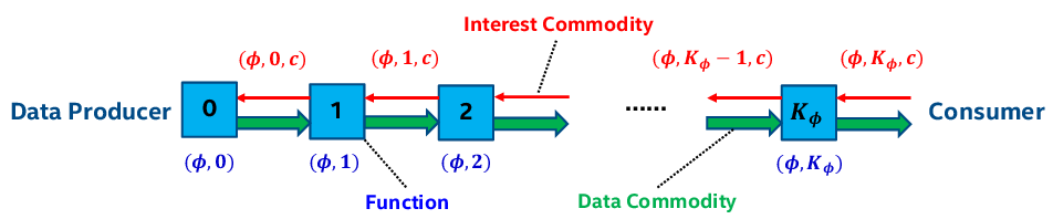
Streams of interest/data packets delivered for a service can be modeled into chaining stages as is shown in Fig. 1. We define each stage of interest packets serving consumer $c\in\mathcal{C}_{\phi}$ requesting for a function $(\phi,k)$ by an interest commodity and use $(\phi,k,c)$ to index it, and with the same index, define each stage of data packets output from function $(\phi,k)$ serving consumer $c$ by a data commodity. In NDN paradigm, the commodity index of an interest/data packet can be inferred from its name, and a processing commitment can updates an interest packet’s commodity by updating it’s name. We let $z^{(\phi,k)}$, $0\leq k\leq K_{\phi}$, represent the size of a data commodity $(\phi,k,c)$ packet for all $c\in\mathcal{C}_{\phi}$, and assume that the network traffic is dominated by the data packets because the size of an interest packet is negligible respective to $z^{(\phi,k)}$.

We define by $a_{c}^{\phi}(t)$ the number of requests for service $\phi$ generated by consumer $c$ at time $t$ and by $\lambda_{c}^{\phi}$ its expected value. We assume that $a_{c}^{\phi}(t)$ is independently and identically distributed (i.i.d) across timeslots, and $\sum\nolimits_{\phi}a_{i}^{\phi}(t)\leq A_{\max}$. At each time $t$, every node buffers the received interest and data packets into queues respectively according to their commodities. Each interest/data queue builds up from the transmission of interest/data packets from neighbors, request/data generations, and/or local processing-commitment/processing. Each node makes local orchestration decisions by controlling the queuing of interest packets, while the data packets are forwarded backward and get processed as committed according to the Pending Interest Table (PIT), and their queues are simply updated in First-In-First-Out mode. Fig. 2 shows an example that a computing node equipped with function $(\phi,k)$ makes decisions on whether or not to commit processing for the arrived interest commodity $(\phi,k,c)$ packets. Once a commitment is made, an interest packet is transported from commodity $(\phi,k,c)$ queue to $(\phi,k-1,c)$ queue with the its commodity index updated.

We define $Q_{i}^{(\phi,k,c)}(t)$ as the number of interest commodity $(\phi,k,c)$ packets queued in node $i$ at the beginning of timeslot $t$; define $b_{ij}^{(\phi,k,c)}(t)$ as the assigned number of interest commodity $(\phi,k,c)$ packets to forward over link $(i,j)$ in timeslot $t$; define $p_{i}^{(\phi,k,c)}(t)$ as the assigned number of interest commodity $(\phi,k,c)$ packets to commit in timeslot $t$ for function $(\phi,k)$. Then node $i$ has the following queuing dynamics:

where $[*]^{+}$ represents $\max\{*,0\}$; $a_{i}^{\phi}(t)\!\!=\!\!0$ if $i\!\notin\!\mathcal{C}_{\phi}$; $p_{i}^{(\phi,k,c)}(t)\!\!=\!\!0$ if $k\!\!>\!\!K_{\phi}$ or $i\!\!\notin\!\!\mathcal{P}_{(\phi,k)}$; $\mathbbm{1}(*)$ is the indicator function of $*$; $p_{i}^{(\phi,k+1,c)}(t)$ is the number of interest commodity $(\phi,k+1,c)$ packets assigned to be transported into commodity $(\phi,k,c)$ queue after being committed by function $(\phi,k+1)$ in timeslot $t$.

The orchestration dynamically controls the action vector $[\{b_{ij}^{(\phi,k,c)}(t)\},\{p_{i}^{(\phi,k,c)}(t)\}]$ subject to the constraints summarized in (2):

where (2a) characterizes the network rate stability [11]; (2b)-(2d) present the capacity constraints for interest forwarding, processing commitment, and data producing. Note that each interest packet flowing over a link eventually results in a data packet flowing backward over the reverse link, and considering that data flow dominates the traffic (see Section II-A), we have (2b) showing that interest packets’ flowing over link $(i,j)$ reflects data packets’ backward flowing constrained by the expected capacity of link $(j,i)$.

For the targeted function chain segment $(\phi,0),\cdots,(\phi,k)$, $0\leq k\leq K_{\phi}$, the discovery interest packets search the resources in order $(\phi,k)\rightarrow\cdots\rightarrow(\phi,0)$, where function $(\phi,k)$ is the immediate searching target. Each discovery interest packet is forwarded by multi-cast. In context NDN, the name of a discovery interest packet $p$ can be $``(\phi,k)\leftarrow\cdots\leftarrow(\phi,0)"$. Once a node having function $(\phi,k)$ is reached by packet $p$, a new discovery interest packet $p^{\prime}$ with name $``(\phi,k-1)\leftarrow\cdots\leftarrow(\phi,0)"$ is generated and multi-cast out to search for function $(\phi,k-1)$. In the meanwhile, packet $p$ is still forwarded out searching for other nodes having function $(\phi,k)$ if its hop limit is not reached, with the purpose of letting the current node know where to offload function $(\phi,k)$’s tasks in the service’s deployment if needed. Fig. 3-3 present the searching phase of a service discovery example.

Fig. 3 shows service discovery for an example function segment $f_{0},f_{1},f_{2}$. Node 1 in Fig. 3 initiates the discovery by generating a discovery interest packet $I_{2}$ with name $``f_{2}\leftarrow f_{1}\leftarrow f_{0}"$, and $I_{2}$ flows to node $2$ having function $f_{2}$. In Fig. 3, node 2 generates a new discovery interest packet $I_{1}$ with name $``f_{1}\leftarrow f_{0}"$, and copies of $I_{1}$ propagate and reach nodes 4 and 7 having function $f_{1}$; $I_{2}$ copies are also forwarded. Fig. 3 shows that both node 4 and 7 generate the packets $I_{0}$ with name $``f_{0}"$, and copies of $I_{0}$ propagate and reach the data producer (node 5). In addition of $I_{2}$’s forwarding, node 4 and 7 forward $I_{1}$ copies that reach each other to prepare for their mutual discovery.

With the purpose of detecting multi-paths, the loop detection used in service discovery is different from the existing mechanism that is used in the standard NDN (see Ref. [7]) based on detecting nonce number collision. The nonce number of each discovery interest packet is updated at each hop to avoid nonce duplication. A loop detection in service discovery enables the discovery interest packet to carry a stop list that records the sequence of IDs of the traveled nodes. If a node having received a discovery interest packet detects that its own node-ID belongs to the packet’s stop list, a looping is identified.

A discovery data packet with name $``(\phi,k)\leftarrow\cdots\leftarrow(\phi,0)"$ is generated in either of the two cases: i) for $k\geq 1$, a node having function $(\phi,k)$ has received/gathered one or multiple discovery data packets with name $``(\phi,k-1)\leftarrow\cdots\leftarrow(\phi,0)"$; ii) for $k=0$, a node having function $(\phi,0)$, i.e., data producer, has received a discovery interest packet with name $``(\phi,0)"$. Each discovery data packet flows backward, i.e., if a discovery data packet with name $``(\phi,k)\leftarrow\cdots\leftarrow(\phi,0)"$ flows over link $(j,i)$, a discovery interest packet with the same name should have flowed over link $(i,j)$. Fig. 3-3 present the feedback phase of the service discovery example.

For the example in Fig. 3, the data producer (node 5) in Fig. 3 generates copies of discovery data packet $D_{0}$ with name $``f_{0}"$ that flow backward until reaching node 4 and 7. In Fig. 3, node 4 and 7 generate the discovery data packets $D_{1}$ with name $``f_{1}\leftarrow f_{0}"$, and $D_{1}$ copies not only flow to node 2 but also flow between node 4 and 7 as their mutual discovery feedback. Fig. 3 shows that node 2 generates discovery data packet $D_{2}$ with name $``f_{2}\leftarrow f_{1}\leftarrow f_{0}"$ that flows back to the discovery initiator (node 1).

We further model implementing a function (or data producing) at a node by going through a “processing link” (or “data producing link”). As is shown in Fig. 4, adding the processing links and data producing links onto a feedback routing path forms an augmented path, which characterizes the trajectory traveled by a relaying series of data packets going through a function chain segment. These discovery data packets gather, update and deliver the minimum abstract distance values along the augmented path, and the path’s abstract distance is calculated by summing the abstract lengths of all the links on it. We measure an abstract link length as follows: i) $l_{ij}\triangleq\nicefrac{{1}}{{\bar{C}_{ji}}}$ for a communication link; ii) $l_{i}^{\text{pr}}=\nicefrac{{r^{(\phi,k)}}}{{z^{(\phi,k)}C_{i}^{\text{pr}}}}$ for a processing link; iii) $l_{i}^{\text{dp}}\triangleq\nicefrac{{1}}{{C_{i}^{\text{dp}}}}$ for a data producing link.

We denote by $L_{i}^{(\phi,k)}$ the minimum abstract distance to travel to node $i$ going through function chain segment $(\phi,0),\cdots,(\phi,k)$. A node $i$ on an augmented path gathers all the discovery data packets during a time window with length $T_{i}^{I}$ (with unit of timeslot) which starts from transmitting a discovery interest packet $I$ with name $``(\phi,k)\leftarrow\cdots\leftarrow(\phi,0)"$, where node $i$ determines the deadline of accepting the discovery data packets based on $T_{i}^{I}$. The $T_{i}^{I}$ value decreases by $1$ timeslot as packet $I$ travels, i.e., $T_{j}^{I}=T_{i}^{I}-1$, if packet $I$ flows over link $(i,j)$. At the end of the time window, node $i$ calculates/updates the minimum abstract distance values, and the updates are shown according to Algorithm 1.

References

• [1] H. Topcuoglu, S. Hariri, and M.-Y. Wu, “Performance-effective and low-complexity task scheduling for heterogeneous computing,” IEEE transactions on parallel and distributed systems, vol. 13, no. 3, pp. 260–274, 2002.
• [2] L. Yang, J. Cao, S. Tang, T. Li, and A. T. Chan, “A framework for partitioning and execution of data stream applications in mobile cloud computing,” in 2012 IEEE Fifth International Conference on Cloud Computing, 2012, pp. 794–802.
• [3] S. Sarkar, S. Chatterjee, and S. Misra, “Assessment of the suitability of fog computing in the context of internet of things,” IEEE Transactions on Cloud Computing, vol. 6, no. 1, pp. 46–59, 2018.
• [4] F. Bonomi, R. Milito, J. Zhu, and S. Addepalli, “Fog computing and its role in the internet of things,” in Proceedings of the first edition of the MCC workshop on Mobile cloud computing, 2012, pp. 13–16.
• [5] R. Pirmagomedov, S. Srikanteswara, D. Moltchanov, G. Arrobo, Y. Zhang, N. Himayat, and Y. Koucheryavy, “Augmented computing at the edge using named data networking,” in 2020 IEEE Globecom Workshops (GC Wkshps), 2020, pp. 1–6.
• [6] T. Refaei, J. Ma, S. Ha, and S. Liu, “Integrating IP and NDN through an extensible IP-NDN gateway,” in Proceedings of the 4th ACM conference on information-centric networking, 2017, pp. 224–225.
• [7] A. Afanasyev and et. al., “NFD developer’s guide,” NDN, Technical Report NDN-0021. https://named-data.net/publications/techreports/, 2021.
• [8] H. Feng, J. Llorca, A. M. Tulino, and A. F. Molisch, “Optimal dynamic cloud network control,” IEEE/ACM Transactions on Networking, vol. 26, no. 5, pp. 2118–2131, 2018.
• [9] K. Kamran, E. Yeh, and Q. Ma, “DECO: Joint computation, caching and forwarding in data-centric computing networks,” in Proceedings of the Twentieth ACM International Symposium on Mobile Ad Hoc Networking and Computing, 2019, pp. 111–120.
• [10] J. Kleinberg and E. Tardos, Algorithm design. Pearson Education India, 2006.
• [11] M. J. Neely, “Stochastic network optimization with application to communication and queueing systems,” Synthesis Lectures on Communication Networks, vol. 3, no. 1, pp. 1–211, 2010.
• [12] ——, “Queue stability and probability 1 convergence via Lyapunov optimization,” arXiv preprint arXiv:1008.3519, 2010.