跳到论文正文
W Papers独立论文阅读器 arXiv:2208.03629 论文正文 计算阅读时间 · 0%
引用这篇论文根据当前论文元数据生成,正式投稿前建议核对。


License: arXiv.org perpetual non-exclusive license
arXiv:2208.03629v1 [gr-qc] 07 Aug 2022

Cosmological perturbations in the spatially covariant gravity with a dynamical lapse function

Xue-Zheng Zhu Email: zhuxzh5@mail2.sysu.edu.cn Affiliation: School of Physics and Astronomy, Sun Yat-sen University, Guangzhou 510275, China    Yang Yu Email: yuyang69@mail2.sysu.edu.cn Affiliation: School of Physics and Astronomy, Sun Yat-sen University, Guangzhou 510275, China    Xian Gao Email: gaoxian@mail.sysu.edu.cn Affiliation: School of Physics and Astronomy, Sun Yat-sen University, Guangzhou 510275, China
Abstract

We investigate the scalar perturbations in a class of spatially covariant gravity theory with a dynamical lapse function. Generally, there are two scalar degrees of freedom due to the presence of the velocity of the lapse function. We treat the scalar perturbations as analogues of those in a two-field inflationary mode, in which one is light mode and the other is the heavy mode. This is justified by the fact that the scalar mode due to the dynamical lapse function becomes infinitely heavy in the limit when the lapse function reduces to be an auxiliary variable. The standard approaches of multiple filed perturbations can be applied to deal with our model. By integrating out the heavy mode and derive the effective theory for the single light field, we find the solution to the single mode in the form of plane waves. Then we calculate the corrections to the power spectrum of the light mode from the heavy mode, by making use of the standard perturbative method of field theory. At last, when the two fields are not weakly coupled, we find a power law mode for the coupled system in large scales.

I Introduction

Inflation is one of the most important ideas in modern cosmology Sato and Yokoyama 2015. In a type model of inflation, one or several scalar fields derive the inflation and generate the quantum fluctuations in the primordial universe.

Inflationary model building also stimulates the study of modified gravity containing additional degrees of freedom beyond the general relativity (GR) (see Clifton et al. 2012; Joyce et al. 2015; Berti et al. 2015 for recent reviews). The Horndeski theory Horndeski 1974; Deffayet et al. 2011; Kobayashi, Yamaguchi, and Yokoyama 2011 is the most general scalar-tensor theory with a single scalar field, in which both the Lagrangian and the equations of motion are up to the second order in derivatives. In recent years, scalar-tensor theories that generalize the Horndeski theory have also been widely investigated Gleyzes et al. 2015a; Gleyzes et al. 2015b; Langlois and Noui 2016; Ben Achour et al. 2016; Crisostomi, Koyama, and Tasinato 2016. An alternative approach to generalizing the scalar-tensor theory is to employ the spatially covariant gravity Gao 2014a; Gao 2014b, which is a metric theory that respect only the spatial covariance. Since the general covariance is broken, it is natural that the lapse function is not an auxiliary variable any more, and also acquires a velocity term N˙\dot{N}. This possibility is considered in Gao and Yao 2019; Gao, Kang, and Yao 2019, which show that there will be an extra scalar mode due to the dynamical lapse function. Usually one has to impose additional conditions in order to remove such an extra mode. On the other hand, from the point of view of the spatially covariant gravity, since the equations of motion of all the modes are of the second order, the extra mode itself is well-behaved. The extra mode loses its dynamics when the lapse function becomes an auxiliary variable, and thus can be treated as a “heavy field”. More precisely, we treat the usual curvature perturbation ζ\zeta as the light mode, and the extra mode AA, which becomes dynamical due to the dynamical lapse function, as the heavy mode. This is the analogue to the well-studied quasi-single field inflation Chen and Wang 2010; Chen and Wang 2012; Noumi, Yamaguchi, and Yokoyama 2013 as well as more general multiple inflation models in which heavy modes are present Cespedes, Atal, and Palma 2012; Achucarro et al. 2012; Burgess, Horbatsch, and Patil 2013; Gao, Langlois, and Mizuno 2012; Gao, Langlois, and Mizuno 2013; Noumi and Yamaguchi 2013; Gao and Gong 2015 (see Chluba, Hamann, and Patil 2015 for a review).

Due to the existence of the coupling terms between the two scalar modes, the perturbations are generally not easy to be solved. In this paper we apply standard methods in multiple field inflation to solving the coupled system and calculate the corrections to the power spectrum of the light mode due to the presence of the heavy mode. First we integrate the heavy mode and derive the effective theory for the light mode Cespedes, Atal, and Palma 2012; Achucarro et al. 2012; Shiu and Xu 2011. We also calculate the influence of the heavy field on the light field by the standard “in-in formalism” of field theory.

When the two fields are not weakly coupled, it will be difficult to using perturbative method of field theory. In this case, we try to solve this coupling system in large scales Tolley and Wesley 2007; Koyama, Mizuno, and Wands 2007.

The rest part of this paper is organized as follows. In Sec. II we described our mode and the cosmological perturbations. In Sec. III we derived the effective theory for the light mode by integrating out the heavy mode. In Sec. IV we calculate the corrections to the power spectrum of the light mode by using the in-in formalism. In Sec. V We discuss the solutions of the coupled system on large scales. In Sec. VI we summarize our analysis.

II Perturbative analysis and the regularization

Let us consider the spatially covariant theories of gravity in Gao, Kang, and Yao 2019

S=∫d​t​d3​x​N​h​(a1​K+a2​F+b1​Ki​j​Ki​j+b2​K2+c1​K​F+c2​F2+d1+d2​R),S=\int\mathrm{d}t\mathrm{d}^{3}x\,N\sqrt{h}\left(a_{1}K+a_{2}F+b_{1}K_{ij}K^{ij}+b_{2}K^{2}+c_{1}KF+c_{2}F^{2}+d_{1}+d_{2}R\right), (1)

where

F:=£𝒏​N=1N​(N˙−£N→​N),\displaystyle F:=\pounds_{\bm{n}}N=\frac{1}{N}\left(\dot{N}-\pounds_{\vec{N}}N\right), (2)
Ki​j:=12​£𝒏​hi​j=12​N​(h˙i​j−£N→​hi​j),\displaystyle K_{ij}:=\frac{1}{2}\pounds_{\bm{n}}h_{ij}=\frac{1}{2N}\left(\dot{h}_{ij}-\pounds_{\vec{N}}h_{ij}\right), (3)

the Ki​jK_{ij} is extrinsic curvature, and NN is lapse function.

The number of the degree of freedom of this model is 4: 2 scalar modes and 2 tensor modes. If we assume the lapse function to be an auxiliary variable, the theory should propagate 3 degrees of freedom. Generally there will be an extra scalar mode due to the presence of FF in the Lagrangian. In Gao, Kang, and Yao 2019, the degenerate condition that leads to only one scalar field has been found. In the current work, we start from the general action (1) and treat it as a model with two scalar modes, which is an analogue of two-field inflation models.

We express spacetime metric in term of the ADM variables

d​s2=−N2​d​t2+hi​j​(d​xi+Ni​d​t)​(d​xj+Nj​d​t),\mathrm{d}s^{2}=-N^{2}\mathrm{d}t^{2}+h_{ij}\left(\mathrm{d}x^{i}+N_{i}\mathrm{d}t\right)\left(\mathrm{d}x^{j}+N^{j}\mathrm{d}t\right), (4)

in this paper we are concerned with the scalar perturbation. We can separate the ADM variables to homogeneous part and perturbations as

N=eA,N=e^{A}, (5)
Ni=a​∂iB,N_{i}=a\partial_{i}B, (6)
hi​j=a2​e2​ζ​δi​j.h_{ij}=a^{2}e^{2\zeta}\delta_{ij}. (7)

Eliminating the BB field that is non-dynamic through the constraint equation, the quadratic action takes the form

S2S=\displaystyle S_{2}^{S}= ∫d​t​d3​x​a3​(−wA​A​A2+gζ​ζ​ζ˙2−1a2​wζ​ζ​(∂ζ)2+wA​ζ​A​ζ˙CLOSE\displaystyle\int\mathrm{d}t\mathrm{d}^{3}x\,a^{3}\left(-w_{AA}A^{2}+g_{\zeta\zeta}\dot{\zeta}^{2}-\frac{1}{a^{2}}w_{\zeta\zeta}(\partial\zeta)^{2}+w_{A\zeta}A\dot{\zeta}\right. (8)
OPEN+gA​A​A˙2+gA​ζ​A˙​ζ˙−1a2​fA​ζ​∂A​∂ζ−1a2​fA​A​(∂A)2).\displaystyle\left.+g_{AA}\dot{A}^{2}+g_{A\zeta}\dot{A}\dot{\zeta}-\frac{1}{a^{2}}f_{A\zeta}\partial A\partial\zeta-\frac{1}{a^{2}}f_{AA}(\partial A)^{2}\right).

The relation between the coefficients in (1) and coefficients in (8) is given in Gao, Kang, and Yao 2019, and shown in A.

Compared to the quadratic action of Horndeski theory, the gA​A​A˙2,gA​ζ​A˙​ζ˙g_{AA}\dot{A}^{2},g_{A\zeta}\dot{A}\dot{\zeta} are new-emerging terms. The degree of freedom of Horndeski theory is 3. But the degree of freedom in our model becomes 4 as the AA field becomes dynamic. The ζ\zeta field is a light field. When we treat the gA​A​A˙2,gA​ζ​A˙​ζ˙g_{AA}\dot{A}^{2},g_{A\zeta}\dot{A}\dot{\zeta} as perturbative terms, the kinetic term is much smaller than the potential term, we think the AA field is a heavy field. For the convenience of calculation, we make various coefficients wA​A,gζ​ζ,wζ​ζ,wA​ζ,gA​ζ,gA​A,fA​ζ,fA​Aw_{AA},g_{\zeta\zeta},w_{\zeta\zeta},w_{A\zeta},g_{A\zeta},g_{AA},f_{A\zeta},f_{AA} as constants that are not function of tt.

It is now convenient to introduce the canonically normalized variables

A=α​1a​A~,ζ=β​1a​ζ~,A=\alpha\frac{1}{a}\tilde{A},\zeta=\beta\frac{1}{a}\widetilde{\zeta}, (9)

the coefficients satisfy

α2​gA​A=12,β2​gζ​ζ=12,\alpha^{2}g_{AA}=\frac{1}{2},\beta^{2}g_{\zeta\zeta}=\frac{1}{2}, (10)

and after using conformal time τ\tau defined by d​t=a​d​τdt=ad\tau, then

S2S=\displaystyle S_{2}^{S}= ∫dτd3x(−a2α2wA​AA~2+α2a′′agA​AA~2+β2a′′agζ​ζζ~2+12ζ~′2\displaystyle\int\mathrm{d}\tau\mathrm{d}^{3}x\,\left(-a^{2}\alpha^{2}w_{AA}\tilde{A}^{2}+\alpha^{2}\frac{a^{\prime\prime}}{a}g_{AA}\tilde{A}^{2}+\beta^{2}\frac{a^{\prime\prime}}{a}g_{\zeta\zeta}\tilde{\zeta}^{2}+\frac{1}{2}\tilde{\zeta}^{\prime}{}^{2}\right.
+12A~′−2α2fA​A(∂A~)2−β2wζ​ζ(∂ζ~)2+αβawA​ζA~ζ~′−αβfA​ζ(∂A~)(∂ζ~)\displaystyle+\frac{1}{2}\tilde{A}^{\prime}{}^{2}-\alpha^{2}f_{AA}\left(\partial\tilde{A}\right)^{2}-\beta^{2}w_{\zeta\zeta}\left(\partial\tilde{\zeta}\right)^{2}+\alpha\beta aw_{A\zeta}\tilde{A}\tilde{\zeta}^{\prime}-\alpha\beta f_{A\zeta}\left(\partial\tilde{A}\right)\left(\partial\tilde{\zeta}\right) (11)
OPEN−α​β​a′​wA​ζ​A~​ζ~+α​β​a′′a​gA​ζ​A~​ζ~+α​β​gA​ζ​A~′​ζ~′).\displaystyle\left.-\alpha\beta a^{\prime}w_{A\zeta}\tilde{A}\tilde{\zeta}+\alpha\beta\frac{a^{\prime\prime}}{a}g_{A\zeta}\tilde{A}\tilde{\zeta}+\alpha\beta g_{A\zeta}\tilde{A}^{\prime}\tilde{\zeta}^{\prime}\right).

III Integrating the heavy mode

The quadratic action for the scalar perturbations takes the form in (8). In the case of GR or the case of usual spatially covariant gravity with one degree of freedom, the lapse function plays as an auxiliary variable with no dynamics. In other words, the coefficients gA​Ag_{AA} and gA​ζg_{A\zeta} are strictly vanishing. This can be equivalently viewed as that AA is infinitely heavy. For the purpose in this work, we relax this requirement by assuming a dynamical lapse function. Nevertheless, we assume the coefficients of the kinetic terms involving AA are small, i.e.,

|gA​AwA​A|≪H−2,|gA​ζwA​A|≪H−2,\left|\frac{g_{AA}}{w_{AA}}\right|\ll H^{-2},\quad\left|\frac{g_{A\zeta}}{w_{AA}}\right|\ll H^{-2}, (12)

the variation of AA is

−2​wA​A​A+wA​ζ​∂tζ−(6​H​gA​A​A˙+2​gA​A​A¨+gA​ζ​ζ¨−2a2​fA​A​∂2A−1a2​fA​ζ​∂2ζ)=0,-2w_{AA}A+w_{A\zeta}\partial_{t}\zeta-\left(6Hg_{AA}\dot{A}+2g_{AA}\ddot{A}+g_{A\zeta}\ddot{\zeta}-\frac{2}{a^{2}}f_{AA}\partial^{2}A-\frac{1}{a^{2}}f_{A\zeta}\partial^{2}\zeta\right)=0, (13)

the mass term of the heavy field is satisfied

mA2=wA​AgA​A,m_{A}^{2}=\frac{w_{AA}}{g_{AA}}, (14)

using (12), the AA can be treated as a heavy field with effective mass much larger than the Hubble scale. Combining with (14), then the (13) takes the form

−2​mA2​gA​A​A+wA​ζ​∂tζ−(6​H​gA​A​A˙+2​gA​A​A¨+gA​ζ​ζ¨−2a2​fA​A​∂2A−1a2​fA​ζ​∂2ζ)=0,-2m_{A}^{2}g_{AA}A+w_{A\zeta}\partial_{t}\zeta-\left(6Hg_{AA}\dot{A}+2g_{AA}\ddot{A}+g_{A\zeta}\ddot{\zeta}-\frac{2}{a^{2}}f_{AA}\partial^{2}A-\frac{1}{a^{2}}f_{A\zeta}\partial^{2}\zeta\right)=0, (15)

for the AA field as a heavy mode, the terms 6​H​gA​A​A˙+2​gA​A​A¨−2a2​fA​A​∂2A6Hg_{AA}\dot{A}+2g_{AA}\ddot{A}-\frac{2}{a^{2}}f_{AA}\partial^{2}A can be neglected Garcia-Saenz, Pinol, and Renaux-Petel 2020, and we choose fA​ζ=0f_{A\zeta}=0 to simplify the calculation, which leads to a restriction on the coefficient d2d_{2}, shown in A (for the case where the coefficient is not 0, we will discuss later). And using the condition that gA​ζg_{A\zeta} is a small parameter, the relation between A and ζ\zeta results from solving its equation of motion at leading order as

A=wA​ζ2​wA​A​∂tζ,A=\frac{w_{A\zeta}}{2w_{AA}}\partial_{t}\zeta, (16)

substituting (16) into the action (8), and neglecting the kinetic gradient and kinetic terms of AA, we obtain the effective Lagrangian

ℒ=wA​ζ24​wA​A​(∂tζ)2+gζ​ζ​(∂tζ)2−1a2​wζ​ζ​(∂ζ)2.\mathcal{L}=\frac{w_{A\zeta}^{2}}{4w_{AA}}\left(\partial_{t}\zeta\right)^{2}+g_{\zeta\zeta}\left(\partial_{t}\zeta\right)^{2}-\frac{1}{a^{2}}w_{\zeta\zeta}\left(\partial\zeta\right)^{2}. (17)

So after this treatment, the two fields becomes a effective single scalar field. Compared to the action of the free part of ζ\zeta field in (8), wA​ζ24​wA​A​(∂tζ)2\frac{w_{A\zeta}^{2}}{4w_{AA}}(\partial_{t}\zeta)^{2} is a new-emerging term. The action is

S2S=∫d​t​d3​x​a3​(wA​ζ24​wA​A​(∂tζ)2+gζ​ζ​(∂tζ)2−1a2​wζ​ζ​(∂ζ)2),S_{2}^{S}=\int\mathrm{d}t\mathrm{d}^{3}x\,a^{3}\left(\frac{w_{A\zeta}^{2}}{4w_{AA}}\left(\partial_{t}\zeta\right)^{2}+g_{\zeta\zeta}\left(\partial_{t}\zeta\right)^{2}-\frac{1}{a^{2}}w_{\zeta\zeta}\left(\partial\zeta\right)^{2}\right), (18)

it is now convenient to introduce the canonically normalized variables

ζ=γ​1a​ζ~,\zeta=\gamma\frac{1}{a}\widetilde{\zeta}, (19)


the coefficients satisfy

γ2​(gζ​ζ+wA​ζ24​wA​A)=12,\gamma^{2}\left(g_{\zeta\zeta}+\frac{w_{A\zeta}^{2}}{4w_{AA}}\right)=\frac{1}{2}, (20)

then the action in (18) will take the form

S2S=∫dτd3x(a′′2​aζ~2+12ζ~′−2γ2wζ​ζ(∂ζ)2),S_{2}^{S}=\int\mathrm{d}\tau\mathrm{d}^{3}x\,\left(\frac{a^{\prime\prime}}{2a}\tilde{\zeta}^{2}+\frac{1}{2}\tilde{\zeta}^{\prime}{}^{2}-\gamma^{2}w_{\zeta\zeta}\left(\partial\zeta\right)^{2}\right), (21)

the equation of motion for the mode function uζu_{\zeta} takes the form

∂2∂τ2​uζ​(k,τ)+2​(k2​γ2​wζ​ζ−a′′2​a)​uζ​(τ,k)=0,\frac{\partial^{2}}{\partial\tau^{2}}u_{\zeta}\left(k,\tau\right)+2\left(k^{2}\gamma^{2}w_{\zeta\zeta}-\frac{a^{\prime\prime}}{2a}\right)u_{\zeta}\left(\tau,k\right)=0, (22)

by seting cζ2=2​γ2​wζ​ζc_{\zeta}^{2}=2\gamma^{2}w_{\zeta\zeta}, and solving in the de Sitter background, we find

uζ​(τ,k)=12​cζ​k​(1−icζ​k​τ)​e−i​cζ​k​τ,\displaystyle u_{\zeta}(\tau,k)=\frac{1}{\sqrt{2c_{\zeta}k}}\left(1-\frac{i}{c_{\zeta}k\tau}\right)e^{-ic_{\zeta}k\tau}, (23)

we calculate the power spectra in the usual way

𝒫ζ=k32​π2​γ2a2​|uζ|2.\mathcal{P}_{\zeta}=\frac{k^{3}}{2\pi^{2}}\frac{\gamma^{2}}{a^{2}}|u_{\zeta}|^{2}. (24)

So the correction of the heavy field to the light field is equivalent to a substitution of γ\gamma to β\beta, the solution to effective theory for the light mode ζ\zeta is still in the form of plane waves, but the propagation speed of the ζ\zeta field has changed.

IV Corrections of the heavy field to the light field

The gA​A​A˙2,gA​ζ​A˙​ζ˙g_{AA}\dot{A}^{2},g_{A\zeta}\dot{A}\dot{\zeta} are new-emerging perturbative terms. We use the perturbation method of field theory to calculate the effect of the heavy AA field on the light ζ\zeta field. For the convenience of calculation, we take fA​ζ=0,f_{A\zeta}=0, wA​ζ=0w_{A\zeta}=0 in action (II), for this kind of non-small coupling terms are not easy to deal with. In our model, when the coefficients gA​Ag_{AA} and gA​ζg_{A\zeta} are not strictly vanishing, it is not easy to quantitatively evaluate the effect of the fA​ζf_{A\zeta} term. If the two fields are both light fields, it is not able to solve motion equations analytically or to integrate out one field. For the two-field model with one light and one heavy modes (heavy enough), or one field is an auxiliary field, we find that the dispersion relation of ζ\zeta field will become complicated, such as appearance of k4k^{4} term. And in Fujita, Gao, and Yokoyama 2016, if AA is completely non-dynamic degree of freedom, and only if fA​ζf_{A\zeta} is constant, the contribution of the coefficient fA​ζf_{A\zeta} to the dispersion relation is mainly the  k4k^{4} term, so it mainly affects the mode with short wavelength, it will be only a correction to the overall magnitude of the power spectrum in large scales. After this treatment, the two fields are weakly coupled, the mode is still a two-field model that a heavy field with a light field. When the two fields are weakly coupled, the perturbative method of field theory can be used to deal with our model.

S2S=\displaystyle S_{2}^{S}= ∫dτd3x(−a2α2wA​AA~2+α2a′′agA​AA~2+β2a′′agζ​ζζ~2+12ζ~′2\displaystyle\int\mathrm{d}\tau\mathrm{d}^{3}x\,\left(-a^{2}\alpha^{2}w_{AA}\tilde{A}^{2}+\alpha^{2}\frac{a^{\prime\prime}}{a}g_{AA}\tilde{A}^{2}+\beta^{2}\frac{a^{\prime\prime}}{a}g_{\zeta\zeta}\tilde{\zeta}^{2}+\frac{1}{2}\tilde{\zeta}^{\prime}{}^{2}\right. (25)
+12A~′−2α2fA​A(∂A~)2−β2wζ​ζ(∂ζ~)2+αβgA​ζA~′ζ~′+αβa′′agA​ζA~ζ~).\displaystyle\left.+\frac{1}{2}\tilde{A}^{\prime}{}^{2}-\alpha^{2}f_{AA}\left(\partial\tilde{A}\right)^{2}-\beta^{2}w_{\zeta\zeta}\left(\partial\tilde{\zeta}\right)^{2}+\alpha\beta g_{A\zeta}\tilde{A}^{\prime}\tilde{\zeta}^{\prime}+\alpha\beta\frac{a^{\prime\prime}}{a}g_{A\zeta}\tilde{A}\tilde{\zeta}\right).

The perturbative terms are

α​β​gA​ζ​A~′​ζ~′+α​β​a′′a​gA​ζ​A~​ζ~.\alpha\beta g_{A\zeta}\tilde{A}^{\prime}\tilde{\zeta}^{\prime}+\alpha\beta\frac{a^{\prime\prime}}{a}g_{A\zeta}\tilde{A}\tilde{\zeta}. (26)

IV.1 Interaction Hamiltonian

In the operator formalism of quantization, we should calculate Hamiltonian in the interaction picture. The Hamiltonian density which is defined by H=πaH=\pi_{a}Qa′Q_{a}^{\prime}-ℒ\mathcal{L}

πA=A~′+gA​ζ​α​β​ζ~′,\pi_{A}=\tilde{A}^{\prime}+g_{A\zeta}\alpha\beta\tilde{\zeta}^{\prime}, (27)
πζ=ζ~′+α​β​gA​ζ​A~′,\pi_{\zeta}=\tilde{\zeta}^{\prime}+\alpha\beta g_{A\zeta}\tilde{A}^{\prime}, (28)

then the Hamiltonian can be written as

H=\displaystyle H= −α2​β2​gA​ζ​wA​ζ​a​A~​πAα2​β2​gA​ζ2−1−πA22​(α2​β2​gA​ζ2−1)−πζ22​(α2​β2​gA​ζ2−1)\displaystyle\frac{-\alpha^{2}\beta^{2}g_{A\zeta}w_{A\zeta}a\tilde{A}\pi_{A}}{\alpha^{2}\beta^{2}g_{A\zeta}^{2}-1}-\frac{\pi_{A}^{2}}{2\left(\alpha^{2}\beta^{2}g_{A\zeta}^{2}-1\right)}-\frac{\pi_{\zeta}^{2}}{2\left(\alpha^{2}\beta^{2}g_{A\zeta}^{2}-1\right)}
+α​β​gA​ζ​πA​πζα2​β2​gA​ζ2−1−α2​β2​wA​ζ2​a2​A~22​(α2​β2​gA​ζ2−1)+α​β​wA​ζ​a​A~​πζα2​β2​gA​ζ2−1\displaystyle+\frac{\alpha\beta g_{A\zeta}\pi_{A}\pi_{\zeta}}{\alpha^{2}\beta^{2}g_{A\zeta}^{2}-1}-\frac{\alpha^{2}\beta^{2}w_{A\zeta}^{2}a^{2}\tilde{A}^{2}}{2\left(\alpha^{2}\beta^{2}g_{A\zeta}^{2}-1\right)}+\frac{\alpha\beta w_{A\zeta}a\tilde{A}\pi_{\zeta}}{\alpha^{2}\beta^{2}g_{A\zeta}^{2}-1} (29)
−α​β​fA​ζ​k2​A~​ζ~+α​β​a′​wA​ζ​A~​ζ~−α​β​gA​ζ​a′′a​A~​ζ~+α2​fA​A​k2​A~2\displaystyle-\alpha\beta f_{A\zeta}k^{2}\tilde{A}\tilde{\zeta}+\alpha\beta a^{\prime}w_{A\zeta}\tilde{A}\tilde{\zeta}-\alpha\beta g_{A\zeta}\frac{a^{\prime\prime}}{a}\tilde{A}\tilde{\zeta}+\alpha^{2}f_{AA}k^{2}\tilde{A}^{2}
+α2​a2​wA​A​A~2−a′′2​a​A~2−12​a′′a​ζ~2+β2​wζ​ζ​k2​ζ~2,\displaystyle+\alpha^{2}a^{2}w_{AA}\tilde{A}^{2}-\frac{a^{\prime\prime}}{2a}\tilde{A}^{2}-\frac{1}{2}\frac{a^{\prime\prime}}{a}\tilde{\zeta}^{2}+\beta^{2}w_{\zeta\zeta}k^{2}\tilde{\zeta}^{2},

HH can be split into two parts, H=H0+HcH=H_{0}+H_{c}, we take the coupling coefficient gA​ζg_{A\zeta}, gA​Ag_{AA}as small parameters, andgA​ζ\ g_{A\zeta}, gA​Ag_{AA} are the same order of magnitude, then

H0=\displaystyle H_{0}= α2​fA​A​k2​A~2+α2​a2​wA​A​A~2−a′′2​a​A~2+12​πA2\displaystyle\alpha^{2}f_{AA}k^{2}\tilde{A}^{2}+\alpha^{2}a^{2}w_{AA}\tilde{A}^{2}-\frac{a^{\prime\prime}}{2a}\tilde{A}^{2}+\frac{1}{2}\pi_{A}^{2} (30)
−12​a′′a​ζ~2+β2​wζ​ζ​k2​ζ~2+12​πζ2,\displaystyle-\frac{1}{2}\frac{a^{\prime\prime}}{a}\tilde{\zeta}^{2}+\beta^{2}w_{\zeta\zeta}k^{2}\tilde{\zeta}^{2}+\frac{1}{2}\pi_{\zeta}^{2},
Hc=−α​β​gA​ζ​a′′a​A~​ζ~−α​β​gA​ζ​πA​πζH_{c}=-\alpha\beta g_{A\zeta}\frac{a^{\prime\prime}}{a}\tilde{A}\tilde{\zeta}-\alpha\beta g_{A\zeta}\pi_{A}\pi_{\zeta} (31)

Where H0H_{0} describes the free part while HcH_{c} describes the cross interactions. From H0H_{0}, the free-theory canonical momenta are related with time-derivatives of the fields as

A~′=∂H0∂πA=πA,\tilde{A}^{\prime}=\frac{\partial H_{0}}{\partial\pi_{A}}=\pi_{A}, (32)
ζ~′=∂H0∂πζ=πζ,\tilde{\zeta}^{\prime}=\frac{\partial H_{0}}{\partial\pi_{\zeta}}=\pi_{\zeta}, (33)

in interaction picture

H0​A=\displaystyle H_{0A}= 12A~′2+α2a2wA​AA~2−a′′2​aA~2\displaystyle\frac{1}{2}\tilde{A}^{\prime}{}^{2}+\alpha^{2}a^{2}w_{AA}\tilde{A}^{2}-\frac{a^{\prime\prime}}{2a}\tilde{A}^{2} (34)
+α2​fA​A​k2​A~2,\displaystyle+\alpha^{2}f_{AA}k^{2}\tilde{A}^{2},
H0​ζ=12ζ~′2−12a′′aζ~2+β2wζ​ζk2ζ~2,H_{0\zeta}=\frac{1}{2}\tilde{\zeta}^{\prime}{}^{2}-\frac{1}{2}\frac{a^{\prime\prime}}{a}\tilde{\zeta}^{2}+\beta^{2}w_{\zeta\zeta}k^{2}\tilde{\zeta}^{2}, (35)
Hc=−α​β​gA​ζ​a′′a​A~​ζ~−α​β​gA​ζ​A~′​ζ~′,H_{c}=-\alpha\beta g_{A\zeta}\frac{a^{\prime\prime}}{a}\tilde{A}\tilde{\zeta}-\alpha\beta g_{A\zeta}\tilde{A}^{\prime}\tilde{\zeta}^{\prime}, (36)

we can write HcH_{c} as

Hc=f1​(τ)​A~​ζ~+f2​A~′​ζ~′,H_{c}=f_{1}(\tau)\tilde{A}\tilde{\zeta}+f_{2}\tilde{A}^{\prime}\tilde{\zeta}^{\prime}, (37)

f1f_{1} is a function of τ\tau, f2f_{2} is a constant.

To canonically quantize the system, the quantum fields are decomposed as

A~​(τ,k)=ak​uA​(τ,k)+a−k†​uA∗​(τ,k),\tilde{A}(\tau,k)=a_{k}u_{A}\left(\tau,k\right)+a_{-k}^{\dagger}u_{A}^{\ast}\left(\tau,k\right), (38)
ζ~​(k,τ)\displaystyle\tilde{\zeta}\left(k,\tau\right) =bk​uζ​(k,τ)+b−k†​uζ∗​(k,τ),\displaystyle=b_{k}u_{\zeta}(k,\tau)+b_{-k}^{\dagger}u_{\zeta}^{\ast}\left(k,\tau\right), (39)

the equations of motion for the mode functions uAu_{A} and uζu_{\zeta} take the form

∂2∂τ2​uA​(τ,k)+2​(α2​a2​wA​A−a′′2​a+α2​fA​A​k2)​uA​(τ,k)=0,\frac{\partial^{2}}{\partial\tau^{2}}u_{A}\left(\tau,k\right)+2\left(\alpha^{2}a^{2}w_{AA}-\frac{a^{\prime\prime}}{2a}+\alpha^{2}f_{AA}k^{2}\right)u_{A}\left(\tau,k\right)=0, (40)
∂2∂τ2​uζ​(k,τ)+2​(k2​β2​wζ​ζ−a′′2​a)​uζ​(τ,k)=0,\frac{\partial^{2}}{\partial\tau^{2}}u_{\zeta}\left(k,\tau\right)+2\left(k^{2}\beta^{2}w_{\zeta\zeta}-\frac{a^{\prime\prime}}{2a}\right)u_{\zeta}\left(\tau,k\right)=0, (41)

then the mass of the heavy mode mAm_{A} can be written as

mA2=2​α2​wA​A,m_{A}^{2}=2\alpha^{2}w_{AA}, (42)

the equation (40) can be rewritten as

∂2∂τ2​uA​(τ,k)+(a2​mA2−a′′a+2​α2​fA​A​k2)​uA​(τ,k)=0.\frac{\partial^{2}}{\partial\tau^{2}}u_{A}\left(\tau,k\right)+\left(a^{2}m_{A}^{2}-\frac{a^{\prime\prime}}{a}+2\alpha^{2}f_{AA}k^{2}\right)u_{A}\left(\tau,k\right)=0. (43)

Where aa and τ\tau are related by a=−1H​τa=-\frac{1}{H\tau}, it is convenient to introduce new variable x≡−2​wζ​ζ​β​k​τx\equiv-\sqrt{2w_{\zeta\zeta}}\beta k\tau and y≡−2​fA​A​α​k​τy\equiv-\sqrt{2f_{AA}}\alpha k\tau, and we take a special case that wζ​ζ=12w_{\zeta\zeta}=\frac{1}{2}, fA​A=12f_{AA}=\frac{1}{2}. The solutions of (41), (43) are

uζ​(x,k)=12​k​β​(1+ix)​ei​x,\displaystyle u_{\zeta}(x,k)=\frac{1}{\sqrt{2k\beta}}\left(1+\frac{i}{x}\right)e^{ix}, (44)
uA​(y,k)=π2​e−π2​ν+i​π4​yk​α​Hi​ν(1)​(y),u_{A}(y,k)=\frac{\sqrt{\pi}}{2}e^{-\frac{\pi}{2}\nu+i\frac{\pi}{4}}\sqrt{\frac{y}{k\alpha}}H_{i\nu}^{(1)}\left(y\right), (45)
ν=mA2H2−94.\nu=\sqrt{\frac{m_{A}^{2}}{H^{2}}-\frac{9}{4}}. (46)

We get Hamiltonian in the interaction picture, and for the part of free field, the solution to the heavy field is in the form of the Hankel function and the solution to the light field is in the form of plane waves.

IV.2 Using in-in formalism for the correction to spectra

We use the field-theoretical perturbative method Gao 2010 to calculate the influence of the new field. For later convenience, we introduce x=1x=1 and y=1y=1 which are their respective values around sound horizon-crossings.

Now we would like to investigate the leading-order corrections to the power spectra. It is interesting to note that the leading-order correction is second-order correction Gao 2010. Thus

𝒫x=1=𝒫x=1(0)+𝒫x=1(2).\mathcal{P}_{x=1}=\mathcal{P}_{x=1}^{(0)}+\mathcal{P}_{x=1}^{(2)}. (47)

The two-point functions for AA and ζ\zeta are defined as

⟨ζ~​(k1,τ1)​ζ~​(k2,τ2)⟩(0)=(2​π)3​δ2​(k1+k2)​Gk​1~​(τ1,τ2),\left\langle\tilde{\zeta}\left(k_{1},\tau_{1}\right)\tilde{\zeta}\left(k_{2},\tau_{2}\right)\right\rangle^{(0)}=\left(2\pi\right)^{3}\delta^{2}\left(k_{1}+k_{2}\right)\tilde{G_{k1}}\left(\tau_{1},\tau_{2}\right), (48)
⟨A~​(k1,τ1)​A~​(k2,τ2)⟩(0)=(2​π)3​δ2​(k1+k2)​Fk​1~​(τ1,τ2),\left\langle\tilde{A}\left(k_{1},\tau_{1}\right)\tilde{A}\left(k_{2},\tau_{2}\right)\right\rangle^{(0)}=\left(2\pi\right)^{3}\delta^{2}\left(k_{1}+k_{2}\right)\tilde{F_{k1}}\left(\tau_{1},\tau_{2}\right), (49)

and

Gk​1~​(τ1,τ2)=uζ​(k,τ)​uζ∗​(k,τ),\tilde{G_{k1}}\left(\tau_{1},\tau_{2}\right)=u_{\zeta}\left(k,\tau\right)u_{\zeta}^{*}\left(k,\tau\right), (50)
Fk​1~​(τ1,τ2)=uA​(k,τ)​uA∗​(k,τ).\tilde{F_{k1}}\left(\tau_{1},\tau_{2}\right)=u_{A}\left(k,\tau\right)u_{A}^{*}\left(k,\tau\right). (51)

The relationship between the expected value of the field before and after the regular transformation

⟨ζ⁡(k1,τ1)​ζ​(k2,τ2)⟩(0)=(2​π)3​δ2​(k1+k2)​Gk​1​(τ1,τ2)=β2a2​⟨ζ~​(k1,τ1)​ζ~​(k2,τ2)⟩(0).\left\langle{\zeta}\left(k_{1},\tau_{1}\right){\zeta}\left(k_{2},\tau_{2}\right)\right\rangle^{(0)}=\left(2\pi\right)^{3}\delta^{2}\left(k_{1}+k_{2}\right){G_{k1}}\left(\tau_{1},\tau_{2}\right)=\frac{{\beta}^{2}}{a^{2}}\left\langle\tilde{\zeta}\left(k_{1},\tau_{1}\right)\tilde{\zeta}\left(k_{2},\tau_{2}\right)\right\rangle^{(0)}. (52)

When gA​Ag_{AA} is much smaller than wA​Aw_{AA}, the model is one heavy field with one light field. The power spectra for light and heavy fields are

𝒫A(0)=k3​α22​π2​H2​τ2​|uA|2,\mathcal{P}_{A}^{(0)}=\frac{k^{3}\alpha^{2}}{2\pi^{2}}H^{2}\tau^{2}|u_{A}|^{2}, (53)
𝒫ζ(0)=k3​β22​π2​H2​τ2​|uζ|2,\mathcal{P}_{\zeta}^{(0)}=\frac{k^{3}\beta^{2}}{2\pi^{2}}H^{2}\tau^{2}|u_{\zeta}|^{2}, (54)

when x=1x=1 at horizon-crossings, we obtain

𝒫ζ(0)=12​β​π2​H2.\mathcal{P}_{\zeta}^{(0)}=\frac{1}{2\beta\pi^{2}}H^{2}. (55)

We only calculate the correction of the heavy field on the light field. The second-order correction is the leading order and in the form

⟨O^​(n)⟩(2)=\displaystyle\left\langle\hat{O}\left(n\right)\right\rangle^{(2)}= −2ℜ∫−∞+τdτ′∫−∞+τ′dτ′′⟨0I|OI^(n)Hc(τ′)Hc(τ′′)|0I(n)⟩\displaystyle-2\Re\int_{-\infty^{+}}^{\tau}d\tau^{\prime}\int_{-\infty^{+}}^{\tau^{\prime}}d\tau^{\prime\prime}\left\langle 0_{I}|\hat{O_{I}}\left(n\right)H_{c}(\tau^{\prime})H_{c}\left(\tau^{\prime\prime}\right)|0_{I}\left(n\right)\right\rangle (56)
+∫−∞−τdτ′∫−∞+τdτ′′⟨0I|Hc(τ′)OI^(n)Hc(τ′′)|0I(n)⟩,\displaystyle+\int_{-\infty^{-}}^{\tau}d\tau^{\prime}\int_{-\infty^{+}}^{\tau}d\tau^{\prime\prime}\left\langle 0_{I}|H_{c}(\tau^{\prime})\hat{O_{I}}\left(n\right)H_{c}\left(\tau^{\prime\prime}\right)|0_{I}\left(n\right)\right\rangle,

according to (37), (56) , we calculate the second-order correction of the AA field to the ζ\zeta field

⟨ζ⁡(τ,k1)​ζ​(τ,k2)⟩(2)=\displaystyle\left\langle{\zeta}\left(\tau,k_{1}\right){\zeta}\left(\tau,k_{2}\right)\right\rangle^{(2)}= (2π)3δ3(k1+k2)×{−4ℜ∫−∞τdτ′∫−∞τ′dτ′′\displaystyle\left(2\pi\right)^{3}\delta^{3}(k_{1}+k_{2})\times\Big\{-4\Re\int_{-\infty}^{\tau}d\tau^{\prime}\int_{-\infty}^{\tau^{\prime}}d\tau^{\prime\prime}
[f22dd​τ′G(τ,τ′)dd​τ′′G(τ,τ′′)dd​τ′dd​τ′′F(τ′,τ′′)+f2f1(τ′′)dd​τ′G(τ,τ′)G(τ,τ′′)dd​τ′F(τ′,τ′′)\displaystyle\Big[f_{2}^{2}\frac{d}{d\tau^{\prime}}G\left(\tau,\tau^{\prime}\right)\frac{d}{d\tau^{\prime\prime}}G\left(\tau,\tau^{\prime\prime}\right)\frac{d}{d\tau^{\prime}}\frac{d}{d\tau^{\prime\prime}}F\left(\tau^{\prime},\tau^{\prime\prime}\right)+f_{2}f_{1}\left(\tau^{\prime\prime}\right)\frac{d}{d\tau^{\prime}}G\left(\tau,\tau^{\prime}\right)G\left(\tau,\tau^{\prime\prime}\right)\frac{d}{d\tau^{\prime}}F\left(\tau^{\prime},\tau^{\prime\prime}\right)
+f1(τ′)f2G(τ,τ′)dd​τ′′G(τ,τ′′)dd​τ′′F(τ′,τ′′)+f1(τ′)f1(τ′′)G(τ,τ′)G(τ,τ′′)F(τ′,τ′′)]\displaystyle+f_{1}\left(\tau^{\prime}\right)f_{2}G\left(\tau,\tau^{\prime}\right)\frac{d}{d\tau^{\prime\prime}}G\left(\tau,\tau^{\prime\prime}\right)\frac{d}{d\tau^{\prime\prime}}F\left(\tau^{\prime},\tau^{\prime\prime}\right)+f_{1}(\tau^{\prime})f_{1}\left(\tau^{\prime\prime}\right)G\left(\tau,\tau^{\prime}\right)G\left(\tau,\tau^{\prime\prime}\right)F\left(\tau^{\prime},\tau^{\prime\prime}\right)\Big]
+2∫−∞τdτ′∫−∞τdτ′′[f22dd​τ′G(τ′,τ)dd​τ′′G(τ,τ′′)dd​τ′dd​τ′′F(τ′,τ′′)\displaystyle+2\int_{-\infty}^{\tau}d\tau^{\prime}\int_{-\infty}^{\tau}d\tau^{\prime\prime}\Big[f_{2}^{2}\frac{d}{d\tau^{\prime}}G\left(\tau^{\prime},\tau\right)\frac{d}{d\tau^{\prime\prime}}G\left(\tau,\tau^{\prime\prime}\right)\frac{d}{d\tau^{\prime}}\frac{d}{d\tau^{\prime\prime}}F\left(\tau^{\prime},\tau^{\prime\prime}\right) (57)
+f2​f1​(τ′′)​dd​τ′​G​(τ′,τ)​G​(τ,τ′′)​dd​τ′​F​(τ′,τ′′)+f1​(τ′)​f2​dd​τ′′​G​(τ,τ′′)​G​(τ′,τ)​dd​τ′′​F​(τ′,τ′′)\displaystyle+f_{2}f_{1}\left(\tau^{\prime\prime}\right)\frac{d}{d\tau^{\prime}}G\left(\tau^{\prime},\tau\right)G\left(\tau,\tau^{\prime\prime}\right)\frac{d}{d\tau^{\prime}}F\left(\tau^{\prime},\tau^{\prime\prime}\right)+f_{1}\left(\tau^{\prime}\right)f_{2}\frac{d}{d\tau^{\prime\prime}}G\left(\tau,\tau^{\prime\prime}\right)G\left(\tau^{\prime},\tau\right)\frac{d}{d\tau^{\prime\prime}}F\left(\tau^{\prime},\tau^{\prime\prime}\right)
+f1(τ′)f1(τ′′)G(τ,τ′′)G(τ′,τ)F(τ′,τ′′)]}.\displaystyle+f_{1}\left(\tau^{\prime}\right)f_{1}\left(\tau^{\prime\prime}\right)G\left(\tau,\tau^{\prime\prime}\right)G\left(\tau^{\prime},\tau)F(\tau^{\prime},\tau^{\prime\prime}\right)\Big]\Big\}.

The leading-order correction to the power spectra of ζ\zeta can be denoted as

⟨ζ⁡(τ,k1)​ζ​(τ,k2)⟩(2)=\displaystyle\left\langle{\zeta}\left(\tau,k_{1}\right){\zeta}\left(\tau,k_{2}\right)\right\rangle^{(2)}= (2​π)3​δ3​(k1+k2)​𝒫ζ(2),\displaystyle\left(2\pi\right)^{3}\delta^{3}(k_{1}+k_{2})\mathcal{P}_{\zeta}^{(2)}, (58)

that

r=αβ=gζ​ζgA​A,r=\frac{\alpha}{\beta}=\sqrt{\frac{g_{\zeta\zeta}}{g_{AA}}}, (59)

inserting (44), (45) into (IV.2), and use the relationship between xx and τ\tau, the second-order correction is

𝒫ζ(2)=r2​e−π​ν​H2​gA​ζ28​k3​β​Γ​(x,r),\mathcal{P}_{\zeta}^{(2)}=r^{2}e^{-\pi\nu}\frac{H^{2}g_{A\zeta}^{2}}{8k^{3}{\beta}}\Gamma\left(x,r\right), (60)

that

Γ⁡(x,r)=\displaystyle\Gamma(x,r)= −4ℜ(1+ix)ei​x(1+ix)ei​x×∫x∞dx′∫x′∞dx′′\displaystyle-4\Re\left(1+\frac{i}{x}\right)e^{ix}\left(1+\frac{i}{x}\right)e^{ix}\times\int_{x}^{\infty}dx^{\prime}\int_{x^{\prime}}^{\infty}dx^{\prime\prime}
(∂∂x′(x′32Hi​ν(1)(x′r))∂∂x′((x′−i)e−i​x′)+2x′Hi​ν(1)(x′r)(1−ix′)e−i​x′)\displaystyle\left(\frac{\partial}{\partial x^{\prime}}\left(x^{\prime^{\frac{3}{2}}}H_{i\nu}^{(1)}\left(x^{\prime}r\right)\right)\frac{\partial}{\partial x^{\prime}}\left(\left(x^{\prime}-i\right)e^{-ix^{\prime}}\right)+2\sqrt{x^{\prime}}H_{i\nu}^{(1)}\left(x^{\prime}r\right)\left(1-\frac{i}{x^{\prime}}\right)e^{-ix^{\prime}}\right)
×(∂∂x′′(x′′32Hi​ν(1)∗(x′′r))∂∂x′′((x′′−i)e−i​x′′)+2x′′Hi​ν(1)∗(x′′r)(1−ix′′)e−i​x′′)\displaystyle\times\left(\frac{\partial}{\partial x^{\prime\prime}}\left(x^{\prime\prime^{\frac{3}{2}}}H_{i\nu}^{(1)\ast}\left(x^{\prime\prime}r\right)\right)\frac{\partial}{\partial x^{\prime\prime}}\left(\left(x^{\prime\prime}-i\right)e^{-ix^{\prime\prime}}\right)+2\sqrt{x^{\prime\prime}}H_{i\nu}^{(1)\ast}\left(x^{\prime\prime}r\right)\left(1-\frac{i}{x^{\prime\prime}}\right)e^{-ix^{\prime\prime}}\right) (61)
+2(1−ix)e−i​x(1+ix)ei​x×∫x∞dx′∫x∞dx′′\displaystyle+2\left(1-\frac{i}{x}\right)e^{-ix}\left(1+\frac{i}{x}\right)e^{ix}\times\int_{x}^{\infty}dx^{\prime}\int_{x}^{\infty}dx^{\prime\prime}
(∂∂x′(x′32Hi​ν(1)(x′r))∂∂x′((x′+i)ei​x′)+2x′Hi​ν(1)(x′r)(1+ix′)ei​x′)\displaystyle\left(\frac{\partial}{\partial x^{\prime}}\left(x^{\prime^{\frac{3}{2}}}H_{i\nu}^{(1)}\left(x^{\prime}r\right)\right)\frac{\partial}{\partial x^{\prime}}\left(\left(x^{\prime}+i\right)e^{ix^{\prime}}\right)+2\sqrt{x^{\prime}}H_{i\nu}^{(1)}\left(x^{\prime}r\right)\left(1+\frac{i}{x^{\prime}}\right)e^{ix^{\prime}}\right)
×(∂∂x′′(x′′32Hi​ν(1)∗(x′′r))∂∂x′′((x′′−i)e−i​x′′)+2x′′Hi​ν(1)∗(x′′r)(1−ix′′)e−i​x′′),\displaystyle\times\left(\frac{\partial}{\partial x^{\prime\prime}}\left(x^{\prime\prime^{\frac{3}{2}}}H_{i\nu}^{(1)\ast}\left(x^{\prime\prime}r\right)\right)\frac{\partial}{\partial x^{\prime\prime}}\left(\left(x^{\prime\prime}-i\right)e^{-ix^{\prime\prime}}\right)+2\sqrt{x^{\prime\prime}}H_{i\nu}^{(1)\ast}\left(x^{\prime\prime}r\right)\left(1-\frac{i}{x^{\prime\prime}}\right)e^{-ix^{\prime\prime}}\right),

and we define

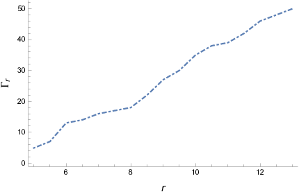
Γr=r2​e−π​ν​Γ​(1,r),\Gamma_{r}=r^{2}e^{-\pi\nu}\Gamma(1,r), (62)

the equation of (IV.2) is a double integral, we will calculate its value at x=1x=1. We find variables except rr can be extracted outside the double integral, so calculating Γr\Gamma_{r} becomes the key to calculating the second-order correction. It is difficult to get an analytical solution, we can only do numerical integration.

Due to the gA​ζg_{A\zeta} is small coefficient, the second-order correction in (60) is a relatively small value. We find that the magnitude of this second-order correction is related to the parameters β,ν,k,r\beta,\nu,k,r. The rr value reflects the relationship between the kinetic energy coefficients of the AA field and the ζ\zeta field, the value of rr in (59) should be quite greater than 1. And the perturbative terms in (26) are related to ratio rr.

Refer to caption
Figure 1: The Γr\Gamma_{r} is defined in (62). We take points within the range of r equal to 5 to 13.

We find that this correction is highly correlated with the ratio rr, the rr value reflects the relationship between the kinetic energy coefficients of the AA field and the ζ\zeta field. We conclude that the Γr\Gamma_{r} increase with the ratio rr.

V Solution in large scales

When using the perturbative method of field theory, the coefficients of the coupling terms in action (8) are small or take the value of 0. In this section, we deal with the case that the coupling coefficient wA​ζw_{A\zeta} is not a small value. We find analytical solutions to the coupled system in large scale. In Tolley and Wesley 2007; Koyama, Mizuno, and Wands 2007, calculating the spectrum under the limit k≪a​Hk\ll aH has been presented.

From the action (II), the equations of motion for the mode functions uAu_{A} and uζu_{\zeta} take the form

−2​a2​α2​wA​A​uA+2​α2​a′′a​gA​A​uA−α​β​a′​wA​ζ​uζ+α​β​a​wA​ζ​uζ′\displaystyle-2a^{2}\alpha^{2}w_{AA}u_{A}+2\alpha^{2}\frac{a^{\prime\prime}}{a}g_{AA}u_{A}-\alpha\beta a^{\prime}w_{A\zeta}u_{\zeta}+\alpha\beta aw_{A\zeta}u_{\zeta}^{\prime}
=∂2∂τ2​uA+k2​(α​β​fA​ζ​uζ+2​α2​fA​A​uA)+α​β​gA​ζ​uζ′′,\displaystyle=\frac{\partial^{2}}{\partial\tau^{2}}u_{A}+k^{2}\left(\alpha\beta f_{A\zeta}u_{\zeta}+2\alpha^{2}f_{AA}u_{A}\right)+\alpha\beta g_{A\zeta}u_{\zeta}^{\prime\prime}, (63)
a′′a​uζ−α​β​a′​wA​ζ​uA+α​β​a′′a​gA​ζ​uA−α​β​a′​wA​ζ​uA−α​β​a​wA​ζ​uA′\displaystyle\frac{a^{\prime\prime}}{a}u_{\zeta}-\alpha\beta a^{\prime}w_{A\zeta}u_{A}+\alpha\beta\frac{a^{\prime\prime}}{a}g_{A\zeta}u_{A}-\alpha\beta a^{\prime}w_{A\zeta}u_{A}-\alpha\beta aw_{A\zeta}u_{A}^{\prime}
=∂2∂τ2​uζ+k2​(2​β2​wζ​ζ​uζ+α​β​fA​ζ​uA)+α​β​gA​ζ​uA′′.\displaystyle=\frac{\partial^{2}}{\partial\tau^{2}}u_{\zeta}+k^{2}\left(2\beta^{2}w_{\zeta\zeta}u_{\zeta}+\alpha\beta f_{A\zeta}u_{A}\right)+\alpha\beta g_{A\zeta}u_{A}^{\prime\prime}. (64)

When a=−1H​τa=-\frac{1}{H\tau}, the condition k≪a​Hk\ll aH leads to k​τ→0k\tau\rightarrow 0, assuming that the equation has a power law solution , meanwhile uAu_{A} and uζu_{\zeta} are same dependence on τ\tau. We assume that the solution to the equation in the following form Tolley and Wesley 2007

uA=B​τp,u_{A}=B\tau^{p}, (65)
uζ=C​τp,u_{\zeta}=C\tau^{p}, (66)

then the terms include k2k^{2} terms can be ignored, substituting (65), (66) into (63), (64), we obtain

−2​1H2​α2​wA​A​B+2​B−α​β​1H​wA​ζ​C−α​β​1H​wA​ζ​p​C=p⁡(p−1)​B+α​β​gA​ζ​p​(p−1)​C,-2\frac{1}{H^{2}}\alpha^{2}w_{AA}B+2B-\alpha\beta\frac{1}{H}w_{A\zeta}C-\alpha\beta\frac{1}{H}w_{A\zeta}pC=p\left(p-1\right)B+\alpha\beta g_{A\zeta}p\left(p-1\right)C, (67)
2​C−2​α​β​1H​wA​ζ​B+2​α​β​gA​ζ​B=p⁡(p−1)​C−α​β​1H​wA​ζ​p​B+α​β​gA​ζ​p​(p−1)​B.2C-2\alpha\beta\frac{1}{H}w_{A\zeta}B+2\alpha\beta g_{A\zeta}B=p\left(p-1\right)C-\alpha\beta\frac{1}{H}w_{A\zeta}pB+\alpha\beta g_{A\zeta}p\left(p-1\right)B. (68)

From (67), (68), we can get the relationship between BB and CC and value of pp. Then we use gA​ζg_{A\zeta} as a small parameter to simplify calculation, there are two sets of solutions, one is

p1=2,p_{1}=2, (69)
B1/C1=−3​β​H​wA​ζ2​α​wA​A,B_{1}/C_{1}=-\frac{3\beta Hw_{A\zeta}}{2\alpha w_{AA}}, (70)

the other is

p2=1/2+(9−8​1H2​α2​wA​A−4​α2​β2​1H2​wA​ζ2)1/2,p_{2}=1/2+\left(9-8\frac{1}{H^{2}}\alpha^{2}w_{AA}-4\alpha^{2}\beta^{2}\frac{1}{H^{2}}w_{A\zeta}^{2}\right)^{1/2}, (71)
B2/C2=p2+1α​β​1H​wA​ζ,B_{2}/C_{2}=\frac{p_{2}+1}{\alpha\beta\frac{1}{H}w_{A\zeta}}, (72)
p3=1/2−(9−8​1H2​α2​wA​A−4​α2​β2​1H2​wA​ζ2)1/2,p_{3}=1/2-\left(9-8\frac{1}{H^{2}}\alpha^{2}w_{AA}-4\alpha^{2}\beta^{2}\frac{1}{H^{2}}w_{A\zeta}^{2}\right)^{1/2}, (73)
B3/C3=p3+1α​β​1H​wA​ζ.B_{3}/C_{3}=\frac{p_{3}+1}{\alpha\beta\frac{1}{H}w_{A\zeta}}. (74)

We find the value of pp is constant or only depends on some coefficients of the model and HH, and the pp has 3 solutions and the corresponding B/CB/C also has 3 solutions. Then

uA=B1​kp1−3/2​(−τ)p1+B2​kp2−3/2​(−τ)p2+B3​kp3−3/2​(−τ)p3,u_{A}=B_{1}k^{p_{1}-3/2}\left(-\tau\right)^{p_{1}}+B_{2}k^{p_{2}-3/2}\left(-\tau\right)^{p_{2}}+B_{3}k^{p_{3}-3/2}\left(-\tau\right)^{p_{3}}, (75)
uζ=C1​kp1−3/2​(−τ)p1+C2​kp2−3/2​(−τ)p2+C3​kp3−3/2​(−τ)p3,u_{\zeta}=C_{1}k^{p_{1}-3/2}\left(-\tau\right)^{p_{1}}+C_{2}k^{p_{2}-3/2}\left(-\tau\right)^{p_{2}}+C_{3}k^{p_{3}-3/2}\left(-\tau\right)^{p_{3}}, (76)

we calculate the power spectra in the usual way

𝒫ζ=k32​π2​β2a2​|uζ|2,\mathcal{P}_{\zeta}=\frac{k^{3}}{2\pi^{2}}\frac{\beta^{2}}{a^{2}}|u_{\zeta}|^{2}, (77)

for de Sitter background, the spectral index is

ns=2​p+1.n_{s}=2p+1. (78)

We find that for the solutions of p​1,p​2,p​3p1,p2,p3, the spectral indices obtained by p​1p1 and p​2p2 are obviously greater than 1, only p​3p3 can achieve a spectral index close to 1, then the coefficients should satisfy

8​1H2​α2​wA​A+4​α2​β2​1H2​wA​ζ2≈354.8\frac{1}{H^{2}}\alpha^{2}w_{AA}+4\alpha^{2}\beta^{2}\frac{1}{H^{2}}w_{A\zeta}^{2}\approx\frac{35}{4}. (79)

From (73), we can change the value of pp by adjusting the parameters in the model, a good pp solution can make spectral index close to 1 in large scales.

VI Conclusions

The spatially covariant gravity with a dynamical lapse function can naturally be viewed as a model with two scalar modes, which is an analogue of two-field inflation model.

In this paper, by regarding the newly-emerging terms as the perturbative terms, we integrate out the heavy mode AA, which arises due to the dynamical lapse function, and get the effective theory for the light mode ζ\zeta, which is the usual curvature perturbation. We find that the propagation speed of ζ\zeta field is modified due to the presence of AA. When the two fields are weakly coupled, the perturbative method of field theory can be used to deal with our model. For the part of free field, we find that the solution to the heavy mode is in the form of Hankel function, and for the light mode the solution is in the form of plane waves. Then we employ the standard in-in formalism to calculate the leading-order corrections to the power spectra of ζ\zeta from the heavy mode AA. Finally, when the two fields are not weakly coupled that the wA​ζw_{A\zeta} is not a small coffecient, we obtain a power law solution as the form τp\tau^{p} in large scales, the index of pp has three solutions, we find that only p​3p3 can lead to a spectral index close to 1.

Acknowledgements

This work was partly supported by the Natural Science Foundation of China (NSFC) under the grant No. 11975020.

Appendix A Coefficients

For the action in (1), the quadratic action for the scalar modes takes the general form

S2S​[ζ,A,B]=∫d​t​d3​x​a3​(L2(1)+L2(2)),S_{2}^{\mathrm{S}}\left[\zeta,A,B\right]=\int\mathrm{d}t\mathrm{d}^{3}x\,a^{3}\left(L_{2}^{(1)}+L_{2}^{(2)}\right), (80)
L2(1)\displaystyle L_{2}^{(1)} =\displaystyle= 𝒞ζ˙2​ζ˙2+𝒞ζ˙​A˙​ζ˙​A˙+𝒞A˙2​A˙2\displaystyle\mathcal{C}_{\dot{\zeta}^{2}}\dot{\zeta}^{2}+\mathcal{C}_{\dot{\zeta}\dot{A}}\dot{\zeta}\dot{A}+\mathcal{C}_{\dot{A}^{2}}\dot{A}^{2} (81)
−𝒞ζ˙​B​ζ˙​∂2Ba−𝒞A˙​B​A˙​∂2Ba+𝒞B2​(∂2B)2a2,\displaystyle-\mathcal{C}_{\dot{\zeta}B}\dot{\zeta}\frac{\partial^{2}B}{a}-\mathcal{C}_{\dot{A}B}\dot{A}\frac{\partial^{2}B}{a}+\mathcal{C}_{B^{2}}\frac{(\partial^{2}B)^{2}}{a^{2}},

terms which are irrelevant to counting the number of degrees of freedom are

L2(2)\displaystyle L_{2}^{(2)} =\displaystyle= 𝒞ζ2​ζ2+𝒞ζ˙​A​ζ˙​A+𝒞ζ​A​ζ​A+𝒞A2​A2−𝒞A​B​A​∂2Ba,\displaystyle\mathcal{C}_{\zeta^{2}}\zeta^{2}+\mathcal{C}_{\dot{\zeta}A}\dot{\zeta}A+\mathcal{C}_{\zeta A}\zeta A+\mathcal{C}_{A^{2}}A^{2}-\mathcal{C}_{AB}A\frac{\partial^{2}B}{a}, (82)

the following coefficients are by Taylor expansion expressed with coefficients in (1), for example, aia_{i} is actually ai​(t,N)|N=1a_{i}\left(t,N\right)|_{N=1}, bib_{i}, cic_{i}, did_{i} are similar cases, the coefficients are

𝒞ζ˙2\displaystyle\mathcal{C}_{\dot{\zeta}^{2}} =\displaystyle= 3​(b1+3​b2),\displaystyle 3(b_{1}+3b_{2}), (83)
𝒞ζ˙​A˙\displaystyle\mathcal{C}_{\dot{\zeta}\dot{A}} =\displaystyle= 3​c1,\displaystyle 3c_{1}, (84)
𝒞A˙2\displaystyle\mathcal{C}_{\dot{A}^{2}} =\displaystyle= c2,\displaystyle c_{2}, (85)
𝒞ζ˙​B\displaystyle\mathcal{C}_{\dot{\zeta}B} =\displaystyle= 2​(b1+3​b2),\displaystyle 2(b_{1}+3b_{2}), (86)
𝒞A˙​B\displaystyle\mathcal{C}_{\dot{A}B} =\displaystyle= c1,\displaystyle c_{1}, (87)
𝒞B2\displaystyle\mathcal{C}_{B^{2}} =\displaystyle= b1+b2,\displaystyle b_{1}+b_{2}, (88)
𝒞ζ2=−2​d2​∂2a2,\mathcal{C}_{\zeta^{2}}=-2d_{2}\frac{\partial^{2}}{a^{2}}, (89)
𝒞ζ˙​A=−3​H​[2​(b1+3​b2)−2​∂(b1+3​b2)∂N+3​c1]+3​(∂a1∂N−a2),\mathcal{C}_{\dot{\zeta}A}=-3H\left[2\left(b_{1}+3b_{2}\right)-2\frac{\partial\left(b_{1}+3b_{2}\right)}{\partial N}+3c_{1}\right]+3\left(\frac{\partial a_{1}}{\partial N}-a_{2}\right), (90)
𝒞ζ​A=−4​(d2+∂d2∂N)​∂2a2,\mathcal{C}_{\zeta A}=-4\left(d_{2}+\frac{\partial d_{2}}{\partial N}\right)\frac{\partial^{2}}{a^{2}}, (91)
𝒞A2\displaystyle\mathcal{C}_{A^{2}} =\displaystyle= −32​∂c1∂N​H˙+12​(d1+3​∂d1∂N+∂2d1∂N2)\displaystyle-\frac{3}{2}\frac{\partial c_{1}}{\partial N}\dot{H}+\frac{1}{2}\left(d_{1}+3\frac{\partial d_{1}}{\partial N}+\frac{\partial^{2}d_{1}}{\partial N^{2}}\right) (92)
+32​H2​[b1+3​b2−∂(b1+3​b2)∂N+∂2(b1+3​b2)∂N2−3​∂c1∂N]\displaystyle+\frac{3}{2}H^{2}\left[b_{1}+3b_{2}-\frac{\partial\left(b_{1}+3b_{2}\right)}{\partial N}+\frac{\partial^{2}\left(b_{1}+3b_{2}\right)}{\partial N^{2}}-3\frac{\partial c_{1}}{\partial N}\right]
+32​H​(∂a1∂N−a2+∂2a1∂N2−∂a2∂N)\displaystyle+\frac{3}{2}H\left(\frac{\partial a_{1}}{\partial N}-a_{2}+\frac{\partial^{2}a_{1}}{\partial N^{2}}-\frac{\partial a_{2}}{\partial N}\right)
−12​[3​H​∂a1∂X+3​∂(b1+3​b2)∂X​H2+∂d1∂X]​∂2a2,\displaystyle-\frac{1}{2}\left[3H\frac{\partial a_{1}}{\partial X}+3\frac{\partial\left(b_{1}+3b_{2}\right)}{\partial X}H^{2}+\frac{\partial d_{1}}{\partial X}\right]\frac{\partial^{2}}{a^{2}},
𝒞A​B=13​𝒞ζ˙​A.\mathcal{C}_{AB}=\frac{1}{3}\mathcal{C}_{\dot{\zeta}A}. (93)

Eliminating the BB field that is non-dynamic through the constraint equation, the quadratic action takes the form

S2S=\displaystyle S_{2}^{S}= ∫d​t​d3​x​a3​(−wA​A​A2+gζ​ζ​ζ˙2−1a2​wζ​ζ​(∂ζ)2+wA​ζ​A​ζ˙CLOSE\displaystyle\int\mathrm{d}t\mathrm{d}^{3}x\,a^{3}\left(-w_{AA}A^{2}+g_{\zeta\zeta}\dot{\zeta}^{2}-\frac{1}{a^{2}}w_{\zeta\zeta}(\partial\zeta)^{2}+w_{A\zeta}A\dot{\zeta}\right. (94)
OPEN+gA​A​A˙2+gA​ζ​A˙​ζ˙−1a2​fA​ζ​∂A​∂ζ−1a2​fA​A​(∂A)2).\displaystyle\left.+g_{AA}\dot{A}^{2}+g_{A\zeta}\dot{A}\dot{\zeta}-\frac{1}{a^{2}}f_{A\zeta}\partial A\partial\zeta-\frac{1}{a^{2}}f_{AA}(\partial A)^{2}\right).

The coefficients for the kinetic terms can be evaluated explicitly to be

gζ​ζ\displaystyle g_{\zeta\zeta} =\displaystyle= 2​b1​(b1+3​b2)b1+b2,\displaystyle\frac{2b_{1}(b_{1}+3b_{2})}{b_{1}+b_{2}}, (95)
gA​ζ\displaystyle g_{A\zeta} =\displaystyle= 2​b1​c1b1+b2,\displaystyle\frac{2b_{1}c_{1}}{b_{1}+b_{2}}, (96)
gA​A\displaystyle g_{AA} =\displaystyle= c2−c124​(b1+b2),\displaystyle c_{2}-\frac{c_{1}^{2}}{4(b_{1}+b_{2})}, (97)
wζ​ζ=−2​d2,w_{\zeta\zeta}=-2d_{2}, (98)
wA​ζ=𝒞ζ˙​A−12​𝒞ζ˙​B​𝒞A​B𝒞B2,w_{A\zeta}=\mathcal{C}_{\dot{\zeta}A}-\frac{1}{2}\frac{\mathcal{C}_{\dot{\zeta}B}\mathcal{C}_{AB}}{\mathcal{C}_{B^{2}}}, (99)
fA​A=−12​[3​H​∂a1∂X+3​∂(b1+3​b2)∂X​H2+∂d1∂X],f_{AA}=-\frac{1}{2}\left[3H\frac{\partial a_{1}}{\partial X}+3\frac{\partial\left(b_{1}+3b_{2}\right)}{\partial X}H^{2}+\frac{\partial d_{1}}{\partial X}\right], (100)
wA​A=\displaystyle w_{AA}= 32​∂c1∂N​H˙−12​(d1+3​∂d1∂N+∂2d1∂N2)\displaystyle\frac{3}{2}\frac{\partial c_{1}}{\partial N}\dot{H}-\frac{1}{2}\left(d_{1}+3\frac{\partial d_{1}}{\partial N}+\frac{\partial^{2}d_{1}}{\partial N^{2}}\right)
−32​H2​[b1+3​b2−∂(b1+3​b2)∂N+∂2(b1+3​b2)∂N2−3​∂c1∂N]\displaystyle-\frac{3}{2}H^{2}\left[b_{1}+3b_{2}-\frac{\partial\left(b_{1}+3b_{2}\right)}{\partial N}+\frac{\partial^{2}\left(b_{1}+3b_{2}\right)}{\partial N^{2}}-3\frac{\partial c_{1}}{\partial N}\right]
−32​H​(∂a1∂N−a2+∂2a1∂N2−∂a2∂N)\displaystyle-\frac{3}{2}H\left(\frac{\partial a_{1}}{\partial N}-a_{2}+\frac{\partial^{2}a_{1}}{\partial N^{2}}-\frac{\partial a_{2}}{\partial N}\right)
+14​𝒞A​B2𝒞B2−14​1a3​∂t(a3​𝒞A​B​𝒞A˙​B𝒞B2),\displaystyle+\frac{1}{4}\frac{\mathcal{C}_{AB}^{2}}{\mathcal{C}_{B^{2}}}-\frac{1}{4}\frac{1}{a^{3}}\partial_{t}\left(a^{3}\frac{\mathcal{C}_{AB}\mathcal{C}_{\dot{A}B}}{\mathcal{C}_{B^{2}}}\right), (101)
fA​ζ=−4​(d2+∂d2∂N),f_{A\zeta}=-4\left(d_{2}+\frac{\partial d_{2}}{\partial N}\right), (102)

for the coefficient fA​ζf_{A\zeta} is equal to 0, we get a relation that −4​(d2+∂d2∂N)|N=1=0-4\left(d_{2}+\frac{\partial d_{2}}{\partial N}\right)|_{N=1}=0. There is no general solution to this case, one of the solutions is d2​(t,N)=c−c​N2d_{2}(t,N)=c-c\frac{N}{2}, where cc is a constant.

References