Van Roosbroeck’s equations with topological terms: the case of Weyl semimetals

Van Roosbroeck’s (VR) system of equationsVan Roosbroeck 1950 comprises the drift-diffusion and continuity equations for electric charge carriers with the Poisson equation for the electric field. These equations have been key for the understanding and development of landmark devices, such as transistors, solar cells and photodiodes. As such, numerous studies and monographs have been published about the VR equations and their solutions (see e.g. Refs. [De Mari 1968; Fonstad 1994; McKelvey 1984; Selberherr 1984; Farrell et al. 2016; Sze et al. 2021]). Modern commercial software packagesMultiphysics 2016 are also equipped to solve the VR equations in a variety of realistic device geometries. Yet, the aforementioned works and software have been tailored to topologically trivial materials.

It is now known that a large fraction of solids host topologically nontrivial electrons Vergniory et al. 2019; Wieder et al. 2022; Vergniory et al. 2022. Thus, there is a marked interest towards creating devices that will exploit the topological properties of matter Liu et al. 2020; Gilbert 2021. Remarkably, although drift-diffusion equations have been used to predict novel electrical transport properties in certain topological materials under restricted (e.g. static) conditions Parameswaran et al. 2014, full-fledged VR equations remain vastly underexploited therein. Little is known about fundamental changes that could emerge in the solutions of those equations when electrons have a nontrivial band topology. If topological microelectronic devices are to become technological reality, such gap of knowledge must be filled. The objective of our paper is to make progress in this direction and to show that VR equations, appropriately adapted to account for nontrivial electronic topology, can unveil new physical effects in topological devices of potential technological interest.

The family of topological materials being large and diverse, we are inclined to make a choice for the purposes of the present study. The material that we focus on is a Weyl semimetal (WSM), where pairs of nondegenerate electronic bands cross at isolated points in the Brillouin zone [Armitage et al. 2018]. These points, called Weyl nodes, are sources or sinks of Berry curvature and have a chirality index $\chi=\pm 1$, which is a topological invariant of the electronic band structure.

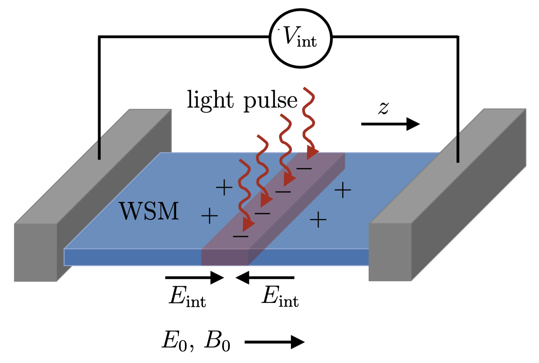
Recently, the investigation and control of WSM using ultrafast light has emerged as a frontier of fundamental and applied research Weber 2021; Bao et al. 2022. On one hand, the influence of the Berry curvature in photodetection and nonlinear optics has been highlighted Golub and Ivchenko 2018; Ahn et al. 2020; Liu et al. 2020; Ma et al. 2021. On the other hand, experiments Jadidi et al. 2020; Levy et al. 2020; Cheng et al. 2021 have measured the light-induced chiral anomaly, a topological property whereby collinear electric and magnetic fields induce a transfer of electrons between Weyl nodes of opposite chirality Burkov 2015.

In this paper, we investigate the interplay between electronic band topology and transient carrier dynamics in a WSM irradiated by a spatially inhomogeneous light pulse (Fig. 1), using a new approach. We begin by writing VR equations for a WSM placed under a strong magnetic field and subject to a light pulse (Sec. II), with adjustments to accommodate for the nontrivial electronic band topology. We follow in Secs. III and IV by linearizing and solving the preceding VR equations. Our strategy of solution is to posit simple but physically justified boundary conditions, and then to take advantage of them by integrating the VR equations over the system’s length. This approach enables us to gain analytical insight for a physical quantity of interest, namely the photovoltage. We thus find a transient photovoltage that oscillates at the plasma frequency. The oscillations originate from the chiral anomaly and are driven by an internal electric field that results from the spatial separation between photoexcited electrons and holes. Unlike in Refs. [Jadidi et al. 2020; Levy et al. 2020; Cheng et al. 2021], the effect of the chiral anomaly is present even when the electric field of light is perpendicular to the static magnetic field. The main text of the paper ends with some discussion (Sec. V) and conclusions (Sec. VI). The six appendices contain technical aspects that allow to reproduce the main results of the paper.

In this section, we adapt the VR equations to a bulk WSM with two nodes. The nodes of opposite chirality are related by symmetry and the energy dispersion is untilted. A strong static and uniform magnetic field ${\bf B}_{0}=B_{0}\hat{\bf z}$ is applied, so that the equilibrium Fermi energy $\epsilon_{F}$ intersects solely with the chiral ($n=0$) Landau levels (Fig. 2). It is in this regime that the effect of chiral anomaly in VR equations is most pronounced. In App.  F, we present the corresponding theory for a weak $B_{0}$.

We restrict our analysis to the electronic dynamics in the $n=0$ and $n=1$ Landau levels. We assume that (i) all the other bands are far enough from $\epsilon_{F}$, and their electronic populations unchanged by the light pulse; (ii) the occupation of the $n=1$ bands in thermal equilibrium is small (low temperature); (iii) the light pulse is uniform across the film thickness and width, but nonuniform along the film length $z$ (Fig. 1). Assumption (iii) justifies the use of one-dimensional VR equations, which we enumerate and discuss next.

In the drift-diffusion approximation, the charge current density along $z$ for the band $(1,\chi)$ is

where $\rho_{1}^{\chi}$ is the electron number density in band $(1,\chi)$, $q$ is the absolute value of the electron’s charge ($q>0$), $E$ is the $z$ component of the total electric field (including a static and uniform electric field $E_{0}$, the electric field of light $E_{\rm light}$, and an internal electric field $E_{\rm int}$ discussed below), $\mu_{1}=q\tau/m^{*}=q|v|\tau l_{B}/(\sqrt{2}\hbar)$ is the mobility of electrons in the $n=1$ band in the effective mass ($m^{*}$) approximation, $|v|$ is the Fermi velocity, $\tau$ is the intraband scattering time in band $(1,\chi)$, $l_{B}=\sqrt{\hbar/(q|B_{0}|)}$ is the magnetic length and $D_{1}=v^{2}\tau$ is the diffusion coefficient. Hereafter, $\tau$ is assumed to be the shortest of all characteristic times in the problem, thereby justifying time-locality in Eq. (1).

The charge current density along $z$ in band $(0,\chi)$ is

where $v=|v|{\rm sgn}(B_{0})$ is the (constant) slope of band $(0,-)$ and $\rho_{0}^{\chi}$ is the electron number density therein. The reason why Eq. (2) looks different from Eq. (1) is that the motion of electrons in a chiral Landau level is one-way. Accordingly, one cannot write the current in a single chiral Landau level as a sum of drift and diffusion currents. This is an example of how electronic band topology requires adjusting the VR equations away from their traditional form. It turns out that the total current in the chiral Landau levels, $j_{0}^{+}+j_{0}^{-}$, can be written in terms of drift and diffusion currents if time variations of the current are slow on the scale of the intervalley relaxation time $\tau_{v}$ (see App.  A). Since we are interested in the dynamics that is faster than $\tau_{v}$, $j_{0}^{+}+j_{0}^{-}$ is not simply a sum of drift and diffusion currents.

The charge continuity equation for band $(n,\chi)$ reads

where

is the $(0,\chi)\to(1,\chi)$ optical generation rate ($g^{\chi}>0$) in units of $1/(\text{time}\times\text{volume})$,

are the relaxation rates for the excess charge in the relaxation time approximation, $\tau_{r}$ is the intravalley electron-hole recombination time and $\rho_{1,\rm eq}^{\chi}$ is the equilibrium electron density in band $(1,\chi)$. We have for simplicity assumed that $\tau_{v}$ is the same for $n=0$ and $n=1$. By considering all relaxation times to be constants, we focus on electron dynamics not far from equilibrium.

The second term in the right hand side (r.h.s.) of Eq. (6) ensures the conservation of the total charge via $\sum_{n,\chi}\left(\partial_{z}j_{n}^{\chi}-q\partial_{t}\rho_{n}^{\chi}\right)=0.$ The third term in the r.h.s. of Eq. (3) is the chiral anomaly term, which in the low-temperature regime enters directly only in the continuity equation for the band intersecting the Fermi level ($n=0$) ¹¹ 1 We neglect the magnetic field of the light pulse and we likewise neglect light-induced lattice strains and their possible contributions Ilan et al. 2020 to the chiral anomaly term.. This term, absent in traditional VR equations, is another example of the adaptation required by nontrivial band topology.

In Eq. (4), $g^{\chi}$ is calculable from Fermi’s golden rule (see App. B). Two properties of $g^{\chi}$ worth noting are that (i) $g^{\chi}\propto|B_{0}|$ due to the Landau level degeneracy, and (ii) $g^{+}(z,t)=g^{-}(z,t)$ if the light pulse preserves the symmetry relating the two Weyl nodes. The latter property fails when $E_{0}\neq 0$, which breaks the $z\to-z$ symmetry. Before light illumination, Eqs. (3), (5) and (6) yield

which implies $\rho_{0}^{+}-\rho_{0}^{-}\propto E_{0}\neq 0$, as though the two Weyl nodes have different chemical potentials. If so, $g^{+}\neq g^{-}$ even when the light pulse preserves the crystal symmetry.

For later reference, the electric current in the absence of a light pulse is obtained from Eq. (7) and reads

where $v_{d}=\mu_{1}E_{0}$ is the drift velocity in $n=1$ bands and

is the dc conductivity from $n=0$ bands.

Lastly, the longitudinal part of the electric field obeys the Poisson equation

where $\epsilon$ is the dielectric constant of the material and the equilibrium charge densities are assumed to be spatially uniform (homogeneous doping).

Because $E_{\rm light}$ is transverse and $E_{0}$ is independent of $z$, $E$ in Eq. (10) equals an internal, photoinduced electric field $E_{\rm int}$. Initially, photoexcited electrons and holes propagate at different speeds due to the markedly different energy dispersions of the $n=0$ and $n=1$ bands. Consequently, a local net charge is generated in the region where the light pulse acts, which in turn produces $E_{\rm int}$. This field tends to neutralize the local charge at times exceeding the dielectric relaxation time.

Neglecting thermoelectric effects Massicotte et al. 2021 for simplicity, Eqs. (1)-(6) and (10) form the complete VR system of equations for the unknowns $\rho_{n}^{\chi}$ and $E$. These nonlinear and coupled equations must in general be solved numerically. Nevertheless, as we show next, analytical insights about the transient optoelectronic response of WSM can be gained by linearizing the VR equations and solving them with simple boundary conditions.

Let us define $\Sigma_{n}\equiv\sum_{\chi}\left(\rho_{n}^{\chi}-\rho_{n,\rm eq}^{\chi}\right)$ and $\Delta_{n}\equiv\sum_{\chi}\chi\left(\rho_{n}^{\chi}-\rho_{n,\rm eq}^{\chi}\right)$ as the deviations of the scalar and chiral electron densities from equilibrium (respectively). For an optical pulse of modest intensity, VR equations can be linearized in $\Sigma_{n}$ and $\Delta_{n}$ (see App. C):

where $g_{s}=\sum_{\chi}g^{\chi}/2$ and $g_{d}=\sum_{\chi}\chi g^{\chi}/2$ are the scalar and chiral optical generation rates (respectively), and

is a characteristic time that emerges from the chiral anomaly term in Eq. (3). Physically, $\epsilon/\sigma_{0}$ is the dielectric relaxation time and $\tau_{a}^{-1}$ is the bulk plasma frequency of chiral electrons (the zero of the $zz$ component of the dielectric tensor) in the absence of scattering Parent et al. 2020.

In Eq. (III), the electron dynamics in the $n=0$ bands is affected by the dynamics in the $n=1$ bands, but not vice versa. Also, the fourth line of Eq. (III) captures the dynamical internodal charge pumping induced by $E_{\rm light}$ by virtue of the chiral anomaly Jadidi et al. 2020; Levy et al. 2020; Cheng et al. 2021. Hereafter, we assume that $E_{\rm light}=0$ (i.e., ${\bf E}_{\rm light}\perp{\bf B}_{0}$). Even then, $E_{\rm int}$ drives a dynamical chiral anomaly because it is collinear to $B_{0}$. Next, we investigate its physical consequence.

Equation (III) can be solved analytically for a WSM film of length $L$ placed between two contacts, and subject to a light pulse that has a finite extent in space and time (Fig. 1). The light pulse is centered at time $t=0$ and the spatial region where it acts is sufficiently far from the contacts. Accordingly, the deviations of the carrier densities with respect to equilibrium vanish when $z\to\pm L/2$ (contact location) or $t\to\pm\infty$. These boundary conditions allow us to solve Eq. (III) by Fourier transform (see App. D). Next, we summarize the approach and the results.

We begin by recognizing that the total electric current density along $z$ can be written as

where the first term in the r.h.s. stands for the particle current and the second term is the displacement current. Out of these parts, the drift current produced by $E_{0}$ is static (Eq. (8)); the remaining parts are induced by the light pulse and are therefore transients.

According to Ampère-Maxwell’s law, the total electric current density must be divergenceless, which in our model amounts to $\partial_{z}J_{\rm tot}=0$ Hawks et al. 2015. Since by construction all transient effects vanish at the contacts, it follows that $J_{\rm tot}$ must be everywhere static and its value given by Eq. (8). In sum, for our boundary conditions, the light pulse has no effect on $J_{\rm tot}$, as though the system were connected to a constant current source.

Contrary to the total current, the voltage drop across the system is influenced by the light pulse. In order to see this, we combine Eqs. (1), (2), (8) and (13) to get

where

is the particle photocurrent. In the limit $\tau_{a}\to 0$, Eq. (III) yields $\Sigma_{0}=-\Sigma_{1}$ (charge neutrality for all $z$ and $t$) and hence $E_{\rm int}=0$. By Eq. (14), $\delta j$ also vanishes when $\tau_{a}\to 0$. This is the ambipolar transport regime Champlain 2011, in which photoexcited electrons of $n=1$ bands and photoexcited holes of $n=0$ bands track each other locally due to electrical attraction, thereby cancelling their currents. For $\tau_{a}\neq 0$, ambipolar transport sets in at $t\gg\tau_{a}$.

Integrating Eq. (14) over the length of the film with the given boundary conditions, we get

where $\overline{f}(t)\equiv\int_{-L/2}^{L/2}dzf(z,t)$ and $V_{\rm int}=-\overline{E_{\rm int}}$ is the transient photovoltage. In Eq. (16), $\overline{\Sigma_{1}}$ and $\overline{\Delta_{0}}$ obey

which are obtained by a spatial integration of Eq. (III). In the first line of Eq. (IV), we have used Eq. (16) to replace $\partial_{t}\overline{E_{\rm int}}$.

To make further progress, we need additional information about the applied light pulse. As such, we consider $\overline{g^{\chi}}(t)$ to be Gaussian with a time width $dt$ and an amplitude $\overline{g_{0}^{\chi}}/(\sqrt{2\pi}dt)$, where $\overline{g_{0}^{\chi}}$ is a constant. Then, a simple analytical solution of Eq. (IV) is realized in the regime $\tau_{a}\ll(\tau_{r},\tau_{v})$ ²² 2 The typical value of $\tau_{a}$ in the quantum limit is $\sim 0.1{\rm ps}$, which is orders of magnitude smaller than $\tau_{v}$ Parameswaran et al. 2014; Jadidi et al. 2020. For $\tau_{r}$, we anticipate (see App. B) a value $\lesssim 1{\rm ps}$. Thus, while $\tau_{a}\ll\tau_{r}$ is reasonable, $\tau_{a}\simeq\tau_{r}$ could also occur. In the latter case, the analytical expression in Eq. (18) is less accurate, but remains in semi-quantitative agreement with the numerical solution of Eq. (IV). and $t\gg dt$ (see App. E). Substituting that solution in Eq. (16), integrating over time and imposing $V_{\rm int}(t\to\infty)=0$, we get

where $\overline{g_{0,s}}=\sum_{\chi}\overline{g_{0}^{\chi}}/2$ and $\overline{g_{0,d}}=\sum_{\chi}\chi\overline{g_{0}^{\chi}}/2$. Figure 3b displays Eq. (18), together with the numerical solution obtained from Eqs. (16) and (IV). Figure 3a shows the photoinduced internal electric field, calculated numerically from Eq. (III).

Eq. (18), the key result of this work, can be interpreted as follows. A light pulse induces a charge separation in the illuminated region and nearby. The resulting electric field, $E_{\rm int}$, creates a neutrality-restoring current through the chiral anomaly, but it overshoots and starts plasma oscillations in the $n=0$ bands. These oscillations are damped by intervalley scattering, which relaxes the current produced by $E_{\rm int}$. If crystal symmetry is preserved, $E_{\rm int}(z)$ is odd in $z$ and thus $V_{\rm int}(t)=0$ (see Fig. 3a and App. D). Breaking the $z\to-z$ symmetry, by either $E_{0}\neq 0$ or by the shape of the light pulse ($\overline{g_{0,d}}\neq 0$), allows for $V_{\rm int}(t)\neq 0$. If the pulse is slow ($dt\gg\tau_{a}$), the ambipolar regime sets in while the sample is being illuminated and $V_{\rm int}$ is suppressed.

Although the oscillations in $V_{\rm int}$ originate from the chiral anomaly, the latter is not required in order to have $V_{\rm int}\neq 0$. We can “turn off” the chiral anomaly in VR equations by taking $\tau_{a}\to\infty$. Experimentally, $\tau_{a}$ can be increased by either reducing $B_{0}$ or by rotating ${\bf B}_{0}$ away from $z$. As soon as $\tau_{a}>\tau_{v}$, the dynamics of $\overline{\Delta_{0}}$ in Eq. (IV) becomes overdamped and hence $V_{\rm int}$ decays monotonically in time (see also App. F).

The appearance of plasma oscillations under light irradiation may seem surprising: bulk plasmons cannot be directly excited by light because they are longitudinal waves, while light waves are transverse (see e.g. Ref. [Barbillon editor]). Yet, our result is enabled by an indirect mechanism: the asymmetric propagation of electrons and holes excited by light generates a longitudinal internal electric field, which can drive plasma oscillations. Furthermore, this mechanism is not unique to topological semimetals: photoinduced plasma oscillations have been observed in semiconductors of trivial band topology Kersting et al. 1997; Kersting et al. 1998; Heyman et al. 2001, where they have attracted much interest as a source of THz radiation. What sets WSM apart is (i) the role of band topology (tunable via ${\bf B}_{0}$), (ii) the ability to attain the quantum limit with modest $B_{0}$, and (iii) the relatively long relaxation time $\tau_{v}$ (due to the relatively large separation in momentum space between counter-moving electrons in the $n=0$ bands).

Let us estimate the magnitude of $V_{\rm int}$. For $B_{0}\simeq 5$T, $|v|\simeq 10^{5}{\rm m/s}$ and $\epsilon=30\epsilon_{0}$ (where $\epsilon_{0}$ is the vacuum permittivity), we have $\tau_{a}\simeq 0.2$ ps. Taking $\tau\simeq 0.1$ ps, we get $\mu_{1}\simeq 0.1~$m${}^{2}{\rm/(Vs)}$. Then, $E_{0}\simeq 1000~{\rm V/m}$ gives $v_{d}\simeq 100~{\rm m/s}$. Using Eq. (9) and $\tau_{v}\simeq~10$ ps, the dc current density is $\simeq 3\times 10^{7}$ A/m². For a WSM film of cross section $100\mu{\rm m}\times 1\mu{\rm m}$, the dc current is modest ($\sim 3\,{\rm mA}$). An optical generation rate of $10^{25}$ pairs/(s cm³) (in App. B we estimate that this rate may be attainable with an optical power of $\sim 1$W), acting during a time $dt\simeq\tau_{a}$ within a length $dz\simeq 100\mu{\rm m}$, gives $\overline{g_{0,s}}\simeq 10^{14}{\rm m}^{-2}$. If $\overline{g_{0,d}}=0$, we arrive at $V_{\rm int}(t)\lesssim 1\mu$V.

There are a few strategies to increase $V_{\rm int}$. First, increasing the power of the optical pulse may be possible, though nonlinear effects neglected in our theory might then need consideration. Second, the use of a $p-n$ junction with a built-in electric field will render $E_{0}$ unnecessary, thereby removing the steady state electric current. Third, in a WSM with multiple pairs of nodes related by time-reversal, each of such pairs will give additive contributions to $V_{\rm int}$. Fourth, in chiral topological semimetals, $\overline{g_{d}}\simeq\overline{g_{s}}$ due to the low crystal symmetry and thus $V_{\rm int}$ could be a factor $|v/v_{d}|\gg 1$ larger than in the estimate of the preceding paragraph (see also Fig. 3b, where $\overline{g_{d}}\neq 0$).

Solving Van Roosbroeck’s equations for topologically nontrivial electronic bands, we have predicted photoinduced plasma oscillations in Weyl semimetals and have elucidated their relation to chiral anomaly. Our findings suggest that it may be interesting to adapt and apply VR equations in order to model a wide variety of topological microelectronic devices.

There are various possible open questions for further work. First, we assumed that the temperature of the system remains constant and uniform under laser irradiation. Yet, this may not be accurate for high laser intensities. What is the influence of electronic band topology in the dynamics and spatial profile of the temperature?

Second, we assumed that the VR equations can be linearized. This requires small departures from equilibrium and therefore limits the scope of our theory. What is the effect of the topological terms in the nonlinear regime of VR equations?

Third, we considered the effect of the chiral anomaly in the VR equations for bulk electrons in a Weyl semimetal. One could study other materials, in which topological quantities should impact the solutions of VR equations.

Fourth, we considered a simple device geometry with simple boundary conditions. If topological microelectronic devices become a technological reality, VR equations augmented with topological terms will need to be solved in more realistic settings using appropriately adapted simulation software.

References

- Van Roosbroeck (1950) W. Van Roosbroeck, The Bell System Technical Journal 29, 560 (1950).
- De Mari (1968) A. De Mari, Solid-State Electronics 11, 1021 (1968).
- Fonstad (1994) C. G. Fonstad, Microelectronic devices and circuits (McGraw-Hill College, New York, 1994).
- McKelvey (1984) J. P. McKelvey, Solid state and semiconductor physics (Robert E. Krieger publishing company, Malabar, Florida, 1984).
- Selberherr (1984) S. Selberherr, Analysis and simulation of semiconductor devices (Springer, New York, 1984).
- Farrell et al. (2016) P. Farrell, N. Rotundo, D. H. Doan, M. Kantner, J. Fuhrmann, and T. Koprucki, Numerical methods for drift-diffusion models, Tech. Rep. (Berlin: Weierstraß-Institut für Angewandte Analysis und Stochastik, 2016).
- Sze et al. (2021) S. M. Sze, Y. Li, and K. K. Ng, Physics of semiconductor devices (John Wiley & sons, 2021).
- Multiphysics (2016) C. Multiphysics, COMSOL Multiphysics (2016).
- Vergniory et al. (2019) M. Vergniory, L. Elcoro, C. Felser, N. Regnault, B. A. Bernevig, and Z. Wang, Nature 566, 480 (2019).
- Wieder et al. (2022) B. J. Wieder, B. Bradlyn, J. Cano, Z. Wang, M. G. Vergniory, L. Elcoro, A. A. Soluyanov, C. Felser, T. Neupert, N. Regnault, et al., Nature Reviews Materials 7, 196 (2022).
- Vergniory et al. (2022) M. G. Vergniory, B. J. Wieder, L. Elcoro, S. S. Parkin, C. Felser, B. A. Bernevig, and N. Regnault, Science 376, eabg9094 (2022).
- Liu et al. (2020) J. Liu, F. Xia, D. Xiao, F. J. Garcia de Abajo, and D. Sun, Nature materials 19, 830 (2020).
- Gilbert (2021) M. J. Gilbert, Communications Physics 4, 70 (2021).
- Parameswaran et al. (2014) S. A. Parameswaran, T. Grover, D. A. Abanin, D. A. Pesin, and A. Vishwanath, Phys. Rev. X 4, 031035 (2014).
- Armitage et al. (2018) N. P. Armitage, E. J. Mele, and A. Vishwanath, Rev. Mod. Phys. 90, 015001 (2018).
- Weber (2021) C. P. Weber, Journal of Applied Physics 129, 070901 (2021), https://doi.org/10.1063/5.0035878 .
- Bao et al. (2022) C. Bao, P. Tang, D. Sun, and S. Zhou, Nature Reviews Physics 4, 33 (2022).
- Golub and Ivchenko (2018) L. E. Golub and E. L. Ivchenko, Phys. Rev. B 98, 075305 (2018).
- Ahn et al. (2020) J. Ahn, G.-Y. Guo, and N. Nagaosa, Phys. Rev. X 10, 041041 (2020).
- Ma et al. (2021) Q. Ma, A. G. Grushin, and K. S. Burch, Nat. Mater. 20, 1601 (2021).
- Jadidi et al. (2020) M. M. Jadidi, M. Kargarian, M. Mittendorff, Y. Aytac, B. Shen, J. C. König-Otto, S. Winnerl, N. Ni, A. L. Gaeta, T. E. Murphy, and H. D. Drew, Phys. Rev. B 102, 245123 (2020).
- Levy et al. (2020) A. L. Levy, A. B. Sushkov, F. Liu, B. Shen, N. Ni, H. D. Drew, and G. S. Jenkins, Phys. Rev. B 101, 125102 (2020).
- Cheng et al. (2021) B. Cheng, T. Schumann, S. Stemmer, and N. P. Armitage, Science Advances 7, eabg0914 (2021).
- Burkov (2015) A. Burkov, Journal of Physics: Condensed Matter 27, 113201 (2015).
- Massicotte et al. (2021) M. Massicotte, G. Soavi, A. Principi, and K.-J. Tielrooij, Nanoscale 13, 8376 (2021).
- Parent et al. (2020) J.-M. Parent, R. Côté, and I. Garate, Phys. Rev. B 102, 245126 (2020).
- Hawks et al. (2015) S. A. Hawks, B. Y. Finck, and B. J. Schwartz, Phys. Rev. Applied 3, 044014 (2015).
- Champlain (2011) J. G. Champlain, Applied Physics Letters 99, 123502 (2011), https://doi.org/10.1063/1.3641898 .
- Barbillon (editor) G. Barbillon (editor), Nanoplasmonics: fundamentals and applications (see chapter by M. Mattheakis, E. Kaxiras and G. P. Tsironis) (BoD–Books on Demand, 2017).
- Kersting et al. (1997) R. Kersting, K. Unterrainer, G. Strasser, H. F. Kauffmann, and E. Gornik, Phys. Rev. Lett. 79, 3038 (1997).
- Kersting et al. (1998) R. Kersting, J. N. Heyman, G. Strasser, and K. Unterrainer, Phys. Rev. B 58, 4553 (1998).
- Heyman et al. (2001) J. N. Heyman, P. Neocleous, D. Hebert, P. A. Crowell, T. Müller, and K. Unterrainer, Phys. Rev. B 64, 085202 (2001).
- Ridley (2013) B. K. Ridley, Quantum processes in semiconductors (Oxford University Press, 2013).
- Griffiths (2014) D. Griffiths, Introduction to Electrodynamics (Pearson Education, 2014).
- Siegman (1986) A. Siegman, Lasers (University Science Books, 1986).
- Rinkel et al. (2019) P. Rinkel, P. L. S. Lopes, and I. Garate, Phys. Rev. B 99, 144301 (2019).
- Son and Spivak (2013) D. T. Son and B. Z. Spivak, Phys. Rev. B 88, 104412 (2013).
- Ilan et al. (2020) R. Ilan, A. G. Grushin, and D. I. Pikulin, Nature Reviews Physics 2, 29 (2020).