Well-posedness and applications of classical elastohydrodynamics for a swimming filament
Abstract.
We consider a classical elastohydrodynamic model of an inextensible filament undergoing planar motion in . The hydrodynamics are described by resistive force theory, and the fiber elasticity is governed by Euler-Bernoulli beam theory. Our aim is twofold: (1) Serve as a starting point for developing the mathematical analysis of filament elastohydrodynamics, particularly the analytical treatment of an inextensibility constraint, and (2) As an application, prove conditions on internal fiber forcing that allow a free-ended filament to swim. Our analysis of fiber swimming speed is supplemented with a numerical optimization of the internal fiber forcing, as well as a novel numerical method for simulating an inextensible swimmer.
1. Introduction
We consider the planar motion of an inextensible, free-ended filament immersed in a Stokes fluid in . The hydrodynamic effects on the filament are described using resistive force theory (or local slender body theory), one of the most fundamental tools for modeling flagellar locomotion in viscous fluids [16, 21, 22, 45]. The structure of the filament itself is described by the classical Euler-Bernoulli beam theory, coupled with internal forcing corresponding to a (possibly nonzero) preferred curvature [19, 61, 62, 3, 2, 48, 18, 49, 55]. Resistive force theory coupled with the elastic response of the fiber has been shown to be remarkably effective at capturing actual filament dynamics, as demonstrated by [8, 64].
Aim 1: Analysis of inextensibility. A key feature of this model is the inextensibility constraint which prohibits the fiber from growing or shrinking in length over time. Inextensibility features prominently in related models of, for example, vesicle dynamics [57, 56, 47], but its treatment is relatively underdeveloped from the perspective of mathematical analysis, particularly in the dynamical setting.
We begin by considering the relaxation of the filament with zero preferred curvature and show global-in-time existence and uniqueness of solutions for small initial data, as well as local well-posedness for large initial data. Global well-posedness for large data is hindered by the behavior of the filament tension. However, we show that if the filament’s initial bending energy is small, then a solution exists globally. As a byproduct, we obtain nonlinear stability of the straight filament. The filament evolution in this setting may be regarded as a simpler version of the Peskin problem (immersed boundary method), which has been the subject of many recent PDE works [13, 14, 29, 40, 54]. This work also follows a recent program by the authors to place nonlocal slender body theory on firm theoretical footing [38, 39, 36, 37, 44]. These previous papers have all considered the static boundary value problem for Stokes flow about a curve at a single instant in time. The form of the integral operator in nonlocal slender body renders the dynamic problem for the curve evolution much more difficult. Using resistive force theory for the force-to-velocity map along the fiber simplifies the curve evolution problem while still remaining relevant from a current modeling perspective (see, for example, [1, 4, 5, 6, 30, 43, 46, 52, 60, 63]).
Aim 2: Analysis of swimming and applications. Resistive force theory coupled with fiber elastodynamics has been especially useful for understanding undulatory swimming at low Reynolds number [7, 9, 10, 20, 34, 26, 24, 51, 27]. This brings us to our second aim: understanding conditions on a filament’s internal forcing which allow it to swim. On the analysis side, we consider the filament dynamics under small-amplitude periodic forcing, corresponding to a nonzero preferred curvature along the fiber. We show existence of a unique periodic solution and derive an expression for the swimming speed of the filament. From the swimming expression, we obtain conditions on the periodic forcing that give rise to propulsion. Our swimming analysis may also be compared to other analysis works on swimming, including [11, 31, 12, 42].
The swimming expression we obtain allows us to perform a small numerical optimization to determine the internal fiber forcing which gives rise to the fastest swimming for a fixed amount of work and bending energy. The optimal forcing that we find is a type of traveling wave; notably, we do not a priori assume any conditions on the forcing other than time periodicity. Our optimization can be compared with related optimizations of the actual filament shape [28, 51, 26, 41, 45], although we emphasize that our optimization is for the active forcing along the filament, and the resulting fiber deformation is an emergent property.
Finally, we develop a novel numerical method based on two recent approaches to inextensibility, due to Moreau et al. [35] and Maxian et al. [32], which rely on different but related methods of avoiding the need to solve for the filament tension. These reformulations of filament elastohydrodynamics are interesting from an analysis perspective because, as seen in the well-posedness results of this paper, estimates for the filament tension are a limiting factor in the solution theory which hinder us in showing global existence for large initial data. A weaker notion of inextensibility – perhaps related to these reformulations – may overcome this difficulty. Moreover, a broader aim of this paper is to serve as a starting point for a full numerical analysis of the various formulations of fiber inextensibility used in numerical simulations, ranging from penalization methods [55] to variants of the more recent approaches which avoid solving for the fiber tension altogether [35, 17, 59, 58, 32, 33]. Our own numerical method is validated against a direct implementation of the classical formulation of filament elastohydrodynamics. We use the method to verify numerically the observations from our swimming analysis.
1.1. Setup and statement of results
We consider an inextensible elastic filament in with centerline parameterized by arclength . Throughout, we will use the subscript to denote differentiation with respect to arclength. The filament is assumed to undergo planar deformations only; in particular, we can define a unique in-plane unit normal vector along the filament centerline. In the presence of active forcing in the form of a preferred curvature , the classical resistive force theory formulation of the evolution of is given by
| (1) | ||||
along with the force-free and torque-free boundary conditions , . For a filament of radius , the constants and for ; in particular, . (Note that some sources define these constants as and ; see, for example, [25, Chapter 6.3]). The hydrodynamic force on the right hand side consists of an elastic term with constant bending stiffness , the unknown tension which serves as a Lagrange multiplier to enforce , and active forcing due to a time-varying preferred curvature along the filament (see [2, 53] or the derivation in Section 3). We will consider both the evolution of a passive filament () and an active filament with time-periodic forcing.
Rescaling arclength as , as , tension as , forcing as , time as , and defining , we may rewrite (1) as
| (2) | ||||
Throughout we will use the notation to denote the unit interval. We also note that the constant . Since the filament is planar and inextensible, the tangent vector at each point may be determined with respect to the angle between and a fixed axis, which we take to be . In particular, we may write
Differentiating the formulation (2) with respect to gives the evolution of the tangent vector . The normal and tangential components of this evolution yield two equations, one for the evolution of the tangent angle and one for the tension at each time:
| (3) | ||||
| (4) | ||||
| (5) |
Note that the boundary conditions for are due to the torque-free condition along with the form of in the force-free condition in (2). The tangent angle formulation (3)-(4), with or without a forcing , is a popular choice for numerical simulations [3, 2, 18, 19, 20, 35, 49, 61, 64]. Given the boundary conditions (5) and the fact that only derivatives of appear on the right hand side of (3) and in the tension equation (4), we find it more convenient to work with the evolution of the filament curvature rather than , as is done in [15, 53]. In particular, given an initial tangent angle , once the curvature evolution is known we may uniquely recover by
| (6) |
Furthermore, it will then be convenient to consider the evolution of the difference as well as . Using equations (3)–(5), we have that and satisfy the equations
| (7) | ||||
| (8) | ||||
| (9) |
The formulation (7)–(9) serves as the basis of our analysis. We will begin by considering the passive filament , for which the dynamics reduce to the simpler system
| (10) | ||||
| (11) | ||||
| (12) |
We define the operator to be the linear evolution of (10) near :
| (13) |
Since the remaining nonlinear terms of (10) are a perfect derivative in , we write the remainder as , where
| (14) |
Letting denote the initial curvature of the fiber, we may define a mild solution to (10) by the Duhamel formula
| (15) |
The fiber curvature in (10)–(12) obeys the energy identity
| (16) |
In particular, is nonincreasing in time. The identity (16) is more easily seen at the level of (2), where sufficiently regular curves satisfy
| (17) |
This may be shown by multiplying both sides of (2) by and integrating in . Integration by parts on the left hand side yields
where we have used the inextensibility constraint .
The system (10)–(12) is invariant under the scaling
Norms which are invariant under the above scaling symmetry are known as critical norms and play an important role in the well-posedness theory. Norms which decay upon ‘zooming in’ via the above scaling are known as subcritical. The natural expectation is that the PDE is (locally) well-posed in subcritical spaces and solutions belonging to subcritical cases are in fact smooth. Typically, if we have a priori control on a subcritical norm for all time, then the solution should be globally well-posed. This is the case for the 1D viscous Burgers’ equation, for example. In our case, any norm with is subcritical. Furthermore, by (16) we have that is monotone decreasing. However, we have found the regularity theory to be much more subtle due to the behavior of the tension (see Remark 2.4 and Section 2.2).11 1 In particular, the local solution to (10)–(12) described in Theorem 1.1 may be extended up to some maximal time depending on the initial data. If the energy identity (16) can be used (in conjunction with a Grönwall argument) to obtain a maximal existence time which depends only on the norm rather than the full initial data, or if it can be shown that, given , the local solution remains in up to time , then the solution can be extended globally. The main difficulty in proving these arises in bounding the tension (see e.g. bound (37)), which seems to necessarily depend on – i.e. a rather high power of a high regularity norm for . This makes the system (10)–(12) somewhat surprising from a regularity point of view. Nevertheless, the energy inequality (16) motivates our choice of function space for the following well-posedness result.
Theorem 1.1 (Well-posedness).
The time weight in (18) allows us to consider rather than . The norm has physical significance, as it is exactly the initial bending energy of the filament. The proof of Theorem 1.1 is given in Section 2. In principle, one can further show that belongs to for all using a bootstrapping argument, although this requires a bit of additional care (see Remark 2.6).
Noting that corresponds to a straight filament, as an immediate corollary of the exponentially decaying bound (18), we obtain:
Corollary 1.2 (Stability of straight fiber).
The straight filament is nonlinearly stable to small perturbations.
We now turn to the filament with active internal forcing in (7)-(9). We take to be time-periodic with period to simulate a waving flagellum. Note that existence and uniqueness of solutions to (7)–(9) with sufficiently small and follow by similar arguments to Theorem 1.1 (see Lemma 3.1). Moreover, we show the existence of a unique -periodic solution :
Theorem 1.3 (Existence of unique periodic solution).
There exist constants and such that, given a -periodic preferred curvature satisfying
there exists a unique -periodic mild solution to the system (7)–(9) satisfying the bound
| (19) |
Furthermore, there exists such that, for any satisfying , the corresponding unique solution to (7)-(9) satisfies
| (20) |
where is the first eigenvalue of the linearized operator (see (30)).
The proof of Theorem 1.3 appears in Section 3.2. Note that by (20), nearby solutions converge very rapidly to the periodic solution. We consider this periodic solution in all further analysis and use it to calculate the fiber swimming speed. To do so, we first must recover the equations for the actual translational motion of the fiber.
Given the unique periodic solution to (7)–(9) and the initial tangent angle , we may uniquely calculate via the equation (6) for . From (6) we may also solve for the frame evolution:
| (21) |
We may then obtain the full evolution of the fiber via
| (22) |
The swimming velocity of the fiber may be calculated as
| (23) |
For suitably small , we seek an expression for the average swimming speed of the fiber in the direction over the course of one period . In what follows, for any function , we will use the notation
| (24) |
to denote the time average over one period. We show the following.
Theorem 1.4 (Small amplitude swimming).
Suppose that is -periodic in time and satisfies
Then a filament whose curvature evolution satisfies (7)-(9) swims with velocity
| (25) |
where and , and is given by
| (26) |
Writing where are the eigenfunctions of the linearized operator (see (30)) and , we have that the time-averaged speed may be written
| (27) | ||||
where are the eigenvalues of and .
The proof of Theorem 1.4 is given in Section 3.3. We note that the additional regularity on is used to ensure that the fiber frame is changing very little over time (see equation (21)). As in previous works (see, e.g., [25]), we obtain that an forcing results in propulsion at most at . From (26), we see that propulsion occurs due to a lag between the actual and preferred curvature of the fiber, which in turn depends on the rate of change of the preferred curvature via (7). However, from (27), we see that further conditions on are needed to actually generate net movement over the course of one full period. Observations about the swimming speed (27) are made more precise in Section 4.1, but may be summarized as follows:
Observations 1.5.
- (1)
Forcing only the lowest nonzero temporal frequency appears to yield the furthest filament displacement for a given amount of work. Thus in further applications we consider the filament’s preferred curvature to be of the form
(28) - (2)
If and are both even or both odd about , the integral in (27) vanishes and the filament does not swim to leading order.
- (3)
Observation (1), which was also noted in [24], comes from numerically solving a simple constrained optimization problem (see (79)). The requirements on and may be considered in terms of the Scallop Theorem for a swimmer in a linear, time-independent flow: violating observation (2) can be seen numerically to lead to a time-reversible filament deformation (see Section 4.3), while violating (3) gives rise to a nearly time-reversible fiber deformation.
A waveform fitting the above criteria is a traveling wave propagating along the filament; for example, and . This is consistent with classical calculations by Pironneau and Katz [45] which find that a filament should deform as a traveling wave to reach a given swimming speed while minimizing energy expenditure.
A further small numerical optimization problem (see (80)) where is constrained as well yields a (28) in the form of a traveling wave which outperforms the simple prescription and . A notable feature of this optimal is that and look like and away from the filament ends, but and at . This is reminiscent of the results of [41], which find that an inactive flagellar endpiece enhances swimming movement.
The above observations are explored in more detail in Section 4.1, and are further supplemented with numerical simulations in Section 4.2. We implement a reformulated version of equation (2) using a novel combination of the methods proposed by Moreau et al. [35] and Maxian et al. [32], which we validate against a direct discretization of (2) (see Appendix A). Using the observations surrounding the form (28) of , we consider combinations of and that give rise to non-swimmers, bad swimmers, and good swimmers, and create visualizations of their respective positions over time.
2. Well-posedness: local for large data, global for small data
2.1. Preliminaries
We begin by stating a few useful lemmas.
Lemma 2.1 (Gagliardo–Nirenberg inequality).
For any function , the following inequality holds for each :
If , then we may replace in the above estimate with .
In addition to Lemma 2.1, we will need estimates for the semigroup generated by the operator (13). We first state some properties of the well-studied Dirichlet problem for the bilaplace equation in 1D (see [23, 61, 62]). In particular, we have explicit expressions for the eigenfunctions and eigenvalues of . First, define an increasing sequence satisfying
| (29) |
The first few values of are given by , , . Note that since increases exponentially as increases, we have as . The eigenfunctions and eigenvalues of are given by
| (30) | ||||
We note in particular that the smallest eigenvalue of is given by . The first six eigenfunctions are plotted in Figure 1. Note that from (30), for odd , is even about , while for even , is odd about .

Using (30), we may define the domain of by
| (31) |
Furthermore, following [50, Chapter 3.7], we may define the domain of fractional powers , , by
| (32) |
Noting the quartic growth of as , we have the following inclusions:
| (33) |
We will repeatedly use the following lemma.
Lemma 2.2 (Semigroup estimates).
Proof.
It remains to show the smoothing estimate, for which we use a duality argument. For , we have
since is self-adjoint. Using (35), we then have
The same result holds for by density. ∎
Finally, we will require the following lemma to show local existence for large initial data.
Lemma 2.3.
Fix and let , . There exists which depends on and satisfies
| (36) |
The smallness in Lemma 2.3 is achieved by approximating by slightly smoother functions.
Proof.
With Lemmas 2.1, 2.2, and 2.3, we may now turn to the proof of Theorem 1.1: well-posedness for the unforced system (10)–(12). First, a remark:
Remark 2.4.
To highlight the subtlety of the well-posedness theory for the system (10)–(12), we may consider the following reduced PDE system consisting of the most problematic terms of (10)–(12):
We may rewrite this simplified system as a single equation:
where is the inverse second derivative with homogeneous Dirichlet conditions at . This equation is invariant under the same scaling symmetry as the full system: . Again, is subcritical for this equation. However, to actually make sense of the tension , we need . Taking initial data only, we expect that due to the smoothing effect of . Thus every which appears in the nonlinear term ‘costs’ . From Lemma 2.2, using the smoothing estimate on the semigroup to account for the outside derivative in the nonlinear term also costs . The nonlinearity then contains three additional powers of , costing a total of . Altogether, we must integrate in the Duhamel formula, so the full power of the smoothing of is required to close the contraction.
2.2. Tension equation
We first consider the elliptic equation (11) and derive the following estimates for the tension in terms of .
Lemma 2.5.
Given , there exists a unique weak solution to equation (11) satisfying
| (37) |
Given , define , to be the solution to (11) using , respectively on the right hand side. The difference then satisfies
| (38) | ||||
Note that the right hand sides of both (37) and (38) involve two powers of an norm, and it is not clear that a lower power is possible. This factor of presents an obstacle to showing global existence for large data, as demonstrated by Remark 2.4.
Proof.
Given , for , we may define
| (39) |
which, due to the sign of the potential term (note that ) is always bounded and coercive on . We may define a weak solution of the tension equation as satisfying
| (40) |
By the Lax–Milgram lemma, there exists a unique weak solution , and, using Lemma 2.1, satisfies
Note that, in terms of regularity, the limiting factor here is the term , which requires 2 powers of to estimate, while the additional regularity of is wasted.
We next show the Lipschitz estimate (38) for . Let , be as defined in Lemma 2.5. The difference then satisfies
Upon multiplying by and integrating by parts in , we obtain
2.3. Evolution equation
We now consider the evolution equation (10) for the curvature . To prove the existence of a unique mild solution (15) in both the large data and small data settings, we will rely on a contraction mapping argument that makes use of the semigroup estimates of Lemma 2.2. We will also require Lemma 2.3 in the large data setting.
Proof of Theorem 1.1.
We begin by defining the function spaces , as
where the norms , , respectively, are given by
We will close a contraction mapping argument in . We consider the intersection of two closed balls in and :
Given either sufficiently small or sufficiently small initial data, we show that the mild solution formula (15) maps into itself for some choice of and .
For any , let denote the mapping
We start by estimating the nonlinear terms of (15). First, using (37) and Lemma 2.1, we have
| (42) | ||||
Here we note that the term from (14) is the limiting factor in terms of regularity (and note that writing and using the smoothing of the semigroup in Lemma 2.2 will still lead to the same result). In particular, since we only have the bound (37) for , the regularity of in this estimate ends up getting wasted, and we end up with 3 powers of on the right hand side of (42).
Then, using Lemma 2.2, for we obtain the following bound:
| (43) | ||||
where we have taken and small enough that .
Furthermore, to obtain a bound, we use that
| (44) | ||||
for sufficiently small. It remains to show that
for which we have two options:
We now show that is a contraction on . For we first note that
| (45) | ||||
Here we have used Lemma 2.1 in the third inequality, and in the fourth we used the estimates (38) and (37) to bound , in terms of , .
Using (45), for we have
and, by a similar series of estimates,
For fixed , taking small enough that both and , by the contraction mapping theorem there exists a unique fixed point of the map in . Furthermore, in the case of small data, combining the bounds (43) and (44), and using that and , we obtain the estimate (18). ∎
Remark 2.6.
Here we sketch a bootstrapping argument for showing that is in fact smooth for all positive times. By a calculation analogous to that above equation (43), it can be shown that in fact belongs to for any positive time. Using this additional regularity on the right hand side of the equation (11) for , we may show that as well. Then, applying to the Duhamel formula (15) for :
since (see (14)), we may use Lemma 2.2 to obtain that for any . Note that we can also show that by applying the full operator above and estimating the integral term in in time.
Passing to higher regularity becomes a bit tricky with the boundary conditions (12): if we were instead working on the torus, we could simply apply , , to the Duhamel formula, and use that commutes with the semigroup . However, on the interval , this requires , which is not necessarily the case since, e.g., does not satisfy the boundary conditions (12).
Instead, we can use that since the right hand side of the equation (10) now belongs to . Taking a time derivative of the equation (10) for , we have
Here satisfies the elliptic equation
and we have that at each time , . Using the Duhamel formula for , we have
where and . Since we need to make sense of , we can again obtain estimates for in a time-weighted space analogous to . In particular, we can estimate
in a similar way as in estimates (43) and (44), and the above argument begins to repeat. Repeating this, we can show that . To obtain spatial regularity from the time regularity, we may use that, once , we have , and, using the equation (10) for , , i.e. .
3. Periodic active forcing and swimming
We now consider the system (7)–(9) with nonzero -periodic active forcing along the filament, corresponding to a nonzero preferred curvature, as derived in [2, 53]. In particular, at a fixed time , let denote the preferred curvature of the fiber. For a planar fiber, recalling that and , we may compute the elastic energy of the fiber as
| (46) | ||||
along with the boundary conditions , , . The Lagrange multiplier is equal to the tension when . Taking the variation and integrating by parts yields
Defining the tension of the fiber to be , we obtain the form of forcing appearing on the right hand side of (2).
3.1. Existence of solution with force
Given the complicated way that the forcing terms due to enter the system (7)–(9), we will first need to establish existence and uniqueness of solutions for for sufficiently small . In particular, we show the following lemma.
Lemma 3.1 (Well-posedness with forcing).
Proof.
We begin by deriving estimates for the forced tension equation (8). Recalling the definition of the bilinear form (39), where now we write , we have that a weak solution of (8) satisfies
| (48) | ||||
Existence of a weak solution again follows by Lax-Milgram, and, using Lemma 2.1 as in the proof of the unforced estimate (37), we have that satisfies
Applying Young’s inequality and again using that , we obtain
| (49) |
We also need to amend the Lipschitz estimate of Lemma 2.5 to account for the presence of the forcing terms. As before, given , , we define and to be the solutions to the forced tension equation (8) using and , respectively, on the right hand side. We have that the difference now satisfies
Proceeding similarly to the proof of Lemma 2.5 and using the bound (49) to estimate the first term involving , we have
Using Lemma 2.1 to absorb the terms into the first expression and applying Young’s inequality, we obtain the Lipschitz bound
| (50) | ||||
Equipped with estimates (49) and (50), we now consider the forced evolution equation (7). We take to be the initial difference from the fiber’s preferred curvature and recall the definition (13) of the operator . We may then write the mild solution formula for (7)–(9), which now consists of three terms:
| (51) |
Here contains all nonlinear terms in equation (7); in particular,
We show that (51) admits a unique fixed point. We define as the space of functions for which the following norm is finite:
| (52) |
Considering a ball of radius in ,
we have that is bounded from to for some . In particular, by Lemma 2.2, the second term of involving satisfies
| (53) | ||||
Furthermore, we may bound the nonlinear terms from following similar steps to the unforced estimate (42) for . Using Lemma (2.1) and the tension estimate (49), we have
| (54) | ||||
By Lemma 2.2, we then have
| (55) | ||||
Combining the estimates (53) and (55) for and , we then have
| (56) |
for . Noting that , we take the preferred curvature and initial condition to satisfy
| (57) |
where , , , and . We then have
| (58) |
for sufficiently small.
We now show that is a contraction on . Given , , we first amend the unforced Lipschitz estimate (45) for to account for the forcing terms in . Using the tension bound (49) and tension Lipschitz estimate (50), as well as Lemma 2.1, we have
Then, using the above estimate along with Lemma 2.2, we have
3.2. Existence of unique periodic solution
We now show that given a -periodic preferred curvature satisfying the smallness assumptions of Lemma 3.1, there exists a unique such that the solution to (7)–(9) is -periodic in time, and solutions starting from nearby initial data converge to this -periodic over time.
Proof of Theorem 1.3.
Given an initial condition and -periodic preferred curvature satisfying the conditions of Lemma 3.1, we consider the unique solution to the system (7)–(9) at time . Let denote the time map :
| (60) |
We consider the map from to and show that there exists a unique fixed point. Here is the ball
where the constant is given by
| (61) |
for , , and as in Lemma 3.1.
We will again make use of the space (52), and note that for , we have
Taking , we first note that, using the bounds (57) and the definition (61) of , the estimate (58) on implies that the second and third terms on the right hand side of (60) satisfy
Next we need a Lipschitz estimate for . Given two initial conditions , , we begin by noting that, by Lemma 2.2, the difference in the linear evolution alone satisfies
Furthermore, using the estimate (59), we may obtain the following bound on the difference in the evolution of the nonlinear terms:
We then have
Noting that , we may subtract from both sides to obtain
| (62) |
In particular, at time we have
which we may rewrite as
| (63) |
Taking the period of the preferred curvature to be large enough that , equation (63) is a contraction on , yielding the unique periodic solution of Theorem 1.3.
As a slight abuse of notation, we now let denote the unique initial condition such that . The estimate (19) then follows from estimate (47) of Lemma 3.1 since we must have . In particular, using the periodicity of , we have
Furthermore, the bound (62) implies that for any initial condition satisfying , the iterated time map satisfies
which yields the convergence estimate (20). ∎
3.3. Swimming
Finally, we calculate the small-amplitude fiber swimming speed stated in Theorem 1.4. The proof will rely on two auxiliary lemmas, which we introduce below.
To show the swimming expression (26), we will need to use the smallness and additional regularity of to show that the fiber tangent vector is not varying greatly in space and time. In particular:
Lemma 3.2.
In addition to Lemma 3.2, in order to show the swimming expansion (27), we will need to consider a nearby simpler problem. We define to be the unique periodic solution to the linear evolution equation
| (65) | ||||
| (66) | ||||
| (67) |
where . The existence of a unique periodic mild solution follows by a simple modification of Section 3.2, and can be shown to satisfy analogous estimates to (49) and (19) for the full system (7)-(9).
For sufficiently small , we have that the unique periodic solution to (7)-(9) is close to the unique periodic :
Lemma 3.3.
Proof of Lemma 3.2.
First, using the Duhamel formula (51) for , by Lemma 2.2 and estimate (55), we may show that
for , due to the additional regularity of . By the periodicity of , we in fact have
Then, using the equation (6) for , we have
Furthermore, using the frame relation , we have that
Combining the above two estimates yields Lemma 3.2. ∎
Proof of Lemma 3.3.
We may use Duhamel’s formula to write the difference as
where is as in (3.1). Recalling that by periodicity, we may replace the space of (52) by in the estimate (55) on the remainder terms . We may use this estimate along with Lemma 2.2 to obtain
| (70) |
Furthermore, using the -periodicity of both and , we have
where we have again used Lemma 2.2. In particular, provided that is large enough that , we have
| (71) |
Combining (70) and (71), we obtain the desired estimate for .
For the tension estimate (69), letting , the difference satisfies
Multiplying by and integrating by parts, we obtain
Proof of Theorem 1.4.
We begin by calculating the form of the swimming velocity stated in equation (23). Using the formulation (2) and recalling that , , and , we have
| (72) | ||||
Here in the second line we have used the boundary conditions in (2), in third line we have replaced with , in the fourth line we have integrated by parts, and in the final line we have added and subtracted .
Then we have that the swimming velocity satisfies
where, using Lemma 3.2, we have
Integration by parts yields the swimming expression (26).
We now consider the equation (65) satisfied by . We aim to use , along with Lemma 3.3, to better understand when expression (26) leads to nonnegligible net motion over one period in time.
Defining , we may first expand and as a Fourier series in time:
| (73) |
Then, using equation (65), the coefficients , , , and satisfy
4. Observations and numerics
In this section, we begin by exploring the observations 1.5 about the swimming speed predicted by the expression (27). We proceed to perform a small numerical optimization of the swimming speed subject to a fixed amount of work performed by the filament. Finally, we outline a numerical method for a reformulation of equation (2) and verify the observations numerically.
4.1. Observations
We first consider the form of the eigenfunctions of (see (30)). Since is odd and is even about for each , we have that eigenfunctions with the same parity do not contribute to net motion:
| (75) |
If is always odd about , we may write
Likewise, if is always even about , we may write
In either of the above cases, due to (75), we have that the leading order term of the swimming expression (27) satisfies
Furthermore, writing
we see that if or either or for all , then the first term in the swimming expression (27) vanishes. Recalling that the eigenvalues of satisfy as and that the smallest eigenvalue (see (30)), we note that this initial term has the greatest relative contribution to filament propulsion. (The remaining terms become relatively more important for large , but the optimimzation results below prompt us to consider only small).
In particular, if this initial term vanishes, the fiber may still have nonzero net motion over the course of one period, but we expect its displacement to be very small.
We may also consider optimizing the swimming speed (27) given certain constraints on the filament deformation, such as a fixed amount of work [51, 25]. We begin by calculating the average work done by the swimmer over one period. Starting with the formulation (2), we have
Here we have used that is -periodic. Using Lemma 3.3, we have that
where, using the expansion (73) and the form of the coefficients (74), we may write
| (76) | ||||
Here we seek to numerically optimize the leading order swimming speed (27) over a (small) finite number of spatial and temporal modes , , subject to a fixed amount of work (76). For a given , , we aim to construct the preferred curvature
which results in the fastest swimming speed. Note that we do not necessarily expect the true optimal preferred curvature to be representable by a finite number of spatial modes , as we cannot construct functions with nonhomogeneous boundary conditions using finitely many eigenfunctions of . We instead aim to visualize general trends in the emerging optimal .
We define the finite-mode swimming speed and work
| (77) | ||||
| (78) |
and solve the following constrained optimization problem for the coefficients , :
| (79) | ||||
Note that we are seeking the fastest swimming speed in the negative direction with respect to the unit tangent vector , i.e. leftward. The optimization is performed using Matlab’s fmincon starting from random initial , satisfying the constraint, where . We use and . For each , the optimal temporal eigenmodes and are plotted in Figure 2(a). As in [24, Section B], we find that forcing only the lowest temporal mode leads to the optimal swimming speed for a given amount of work. Notably, the optimal is perfectly odd about while is perfectly even. The phase difference between and is consistent with the classical optimization paper [45] which finds that, to reach a given swimming speed while minimizing energy expenditure, the filament should deform as a traveling wave.


Note that for small , the expression for average work (76) is essentially the norm of along the length of the filament, due to the coefficient of the summand. Thus, given a fixed amount of work, we expect the optimal to oscillate at the highest allowable frequency in , as seen in Figure 2(a). Constraining only the work done by the filament thus may not lead to the most physically realistic optimum. As noted in [28, 51], the bending energy of the filament can also be taken into account.
Thus we also consider the additional constraint const., and solve the following optimization problem for the coefficients , :
| (80) | ||||
Due to the results of optimization problem (79), we take and optimize only over spatial modes . Two different results of the optimization for are plotted in Figures 2(b) and 2(c). Both yield the same swimming speed .
Case (B) is similar to a simple sine and cosine, i.e. perhaps the most familiar traveling wave example. However, since and are constructed of finitely many eigenfunctions (see (30)), they are constrained to have homogeneous boundary conditions. We also note the striking symmetry in the solutions of case (C).
4.2. Numerical method
Here we numerically verify the swimming predictions of the previous section. We develop a simple numerical method for simulating the motion of an inextensible filament via resistive force theory based on a combination of the methods of [32] and [35]. We apply the method to the planar swimmer studied in the previous sections, but note that the formulation itself is applicable more generally.
While the curvature evolution equations (7)-(9) in terms of and are convenient for analysis, a direct numerical implementation can be cumbersome due in part to complicated dependence on the forcing as well as the need to solve for the actual fiber movement separately (22). Numerically, however, we can make use of reformulations that may simplify the computation. As noted, our future goal is to do numerical analysis comparing the many existing formulations of filament inextensibility.
To introduce the numerical method, we return to the original formulation of inextensible fiber dynamics (2), which we reiterate here for convenience:
| (81) | ||||
We enforce inextensibility directly by parameterizing as
| (82) |
where ; in particular, .
Along the fiber we may rewrite (81) as the coupled system
| (83) | ||||
| (84) |
where is the hydrodynamic force density along the filament, and only the normal components of the integrated force density (84) are specified. To satisfy the boundary conditions of (81), we must also ensure that the total hydrodynamic force and torque along the fiber vanish:
| (85) |
The formulation (83)-(84), combined with total force vanishing (85), is equivalent to the formulation in [32], which uses slender body theory rather than resistive force theory in equation (83). As noted in [32], equations (83)-(84) along with (85) are enough to recover the rate of work exerted by the filament on the fluid in (81). In particular, the rate of work may be calculated using (83)-(84) as
where we have integrated by parts and used that . Starting instead from (81) and again integrating by parts and using , we also obtain
Since we are using resistive force theory, equation (83) may be directly inverted to solve for :
| (86) |
and this expression may be inserted into (84) to condense (83) and (84) into a single equation along the filament. For a planar fiber, recalling that we may parameterize , , and that , we may rewrite (83) and (84) as
| (87) |
Equation (87) will be the main evolution equation for the fiber, for which the unknowns are the basepoint and the tangent angle . We combine (87) with the total force balance (85) to enforce the boundary condition :
| (88) |
The torque condition in (85) leads to the boundary condition , which will be enforced directly in the discretization of on the right hand side of (87).
The fiber is discretized into segments between points along the fiber, and , , is taken to be the angle between segment and the -axis (see Figure 3). The equation (87) is enforced at the midpoint of each segment at , .
As mentioned, the boundary condition is enforced in the discretization of on the right hand side of (87) via the approximation
| (89) |
At the endpoint, equations (87) and (88) coincide to yield the boundary condition , which, using (89), yields an equation for :
| (90) |
The full discretized system is then given by
| (91) | ||||
| (92) | ||||
| (93) |
along with equation (90). Here the evolution of each segment midpoint is parameterized as
and the matrix is given by
The expressions (91) and (92) include equations enforced at ; the expression (93) involves two equations enforced at ; and the equation (90) gives one additional equation to uniquely determine the unknowns , , , …, . We use a standard ODE solver to evolve (90)–(93) in time.
The formulation (90)–(93) is very similar to that of Moreau et al. [35], which also avoids the need to solve for the unknown tension by projecting away from the tangential direction along the fiber. At the continuous level, the formulation in [35] is essentially based on the identity
| (94) |
Integrating (94) with respect to arclength from to 1 () and using the boundary conditions in (81), the identity (94) yields
| (95) | ||||
In the case of a planar filament parameterized by the tangent angle , we have . Combining (95) with the definition of (86), we obtain (in the direction):
| (96) | ||||
The equation (96) is also enforced at each of the midpoints along the discretized fiber (see Figure 3). To close the discretized system, equation (96) is accompanied by the total force constraint
| (97) |
which gives two additional equations.
4.3. Swimmer numerics
We use the numerical method (90)–(93) to test the swimming predictions from Section 4.1. In each simulation, the initial condition is a straight fiber lying on the -axis from to . We discretize the fiber into segments and prescribe a preferred curvature of the form
Temporal forcing is only at the lowest mode, in accordance with the conclusions of the previous section. We take and , and consider different waveforms and .
Non-swimmers: We begin by considering combinations of and which are predicted to produce no net motion over each time period. In accordance with the observations of Section 4.1, we consider examples where and are either both even or both odd about . Specifically, we take
- (1)
, (both even about )
- (2)
, (both odd about )
and normalize both such that . The two combinations of and are plotted in Figure 4, along with snapshots of the spatial positions of both swimmer (1) and swimmer (2) over the course of 50 time units. As predicted, neither swimmer exhibits net displacement in the -direction.


Bad swimmers: We next consider swimmers predicted in Section 4.1 to possibly swim, but very poorly. We choose to be neither even nor odd about , and consider and :
- (3)
,
- (4)
,
- (5)
, .
As before, we normalize . The three combinations of and are plotted in Figure 5, along with snapshots of their corresponding fiber positions over the course of 50 time units. Note that all three exhibit a very small rightward displacement.


Good swimmers: Finally, we consider four examples of swimmers which do exhibit nonnegligible net motion, in accordance with the observations of Section 4.1. We consider the following four combinations of and :
In each case, and are normalized to have . Snapshots of each swimmer’s position over 50 time units are plotted in Figure 6. Notably, all four swimmers swim relatively well, but the two optimal swimmers from Figure 2 swim the farthest.


We may compare the swimming distance predicted by the expression (26) to the observed displacement of the swimmer over a few periods. We numerically calculate the integral
over the course of 5 time units between and . In Table 1, we compare this integral expression to the actual horizontal displacement of the swimmer observed in numerical simulations, which we calculate as . Note that in cases (8) and (9), the distance is far less than the predicted by the linear theory. The prescribed is not small, so nonlinear effects impact the swimming speeds seen here.
| Predicted displacement | Observed displacement | |
|---|---|---|
| Case 6 | -0.06033 | -0.06013 |
| Case 7 | 0.02643 | 0.02652 |
| Case 8 | -0.1201 | -0.1204 |
| Case 9 | -0.1226 | -0.1220 |
Finally, in one representative case each of non-swimmer, bad swimmer, and good swimmer, we plot the integrand of the swimming expression (26) as a function of arclength over the course of one time period. Figure 7 displays snapshots of this integrand for forcing functions (1), (3), and (6), respectively.


In case (1), we note that the integrand is odd about at each time step and hence integrates to zero along the length of the filament, leading to no net motion due to spatial symmetry. In case (3), we see that does not integrate to zero in but very nearly integrates to zero in time. The (near) lack of displacement here can be attributed to time symmetry. Finally, in case (6) the function clearly integrates to a positive number in space and time, leading to net motion (note that the displacement is negative according to the sign of (26)).
Appendix A Validation of numerical method
We validate the numerical method for the formulation described in Section 4.2 through comparison with a direct discretization of the classical inextensible fiber formulation (81).
The implementation of (81) requires description. We first rewrite the system (81) as follows:
| (98) | ||||
Our spatial discretization is as in Figure 3, and we denote the arclength coordinate by where . Let us also define the midpoints . Let be the discretization of and be the discretization of . As the notation suggests, are seen as residing at whereas reside at the midpoints . Our unknowns are and . First, set:
| (99) |
Using the above expressions, define:
We thus obtain the following semi-discretized system:
| (100) |
Notice that this is a differential algebraic system for and , and there are exactly equations matching the number of unknown functions. We discretize the above equation in time as follows. We let be the time step. Let and denote the values of and evaluated at time . Our time discretization is essentially a backward Euler method in which some parts of the equation are treated explicitly. Given , we solve the following system of equations to find and :
| (101) |
In the above, and are computed with using the second line of equation (99).
Note also that and hence are known quantities.
The above constitute equations in the unknowns and . These equations are solved using Newton’s method.
Hereafter we will refer to the method (90)–(93) as Method (a), and the method (101) as Method (b), and denote the corresponding fiber configurations by and , respectively.
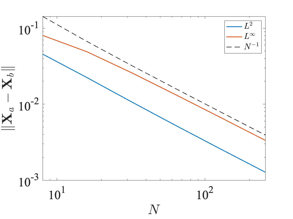
We begin by comparing the methods in the case of zero preferred curvature . The initial filament configuration is a semicircle, and the fiber rapidly relaxes into a straight line. In Figure 8(a) we evolve the fiber until time and plot the norm of the difference between Method (a) and Method (b) as the number of fiber segments is increased. We plot the and norms of the difference , which both display convergence. In Figure 8(b) we plot the actual fiber configurations (blue) and (red) at different times for .

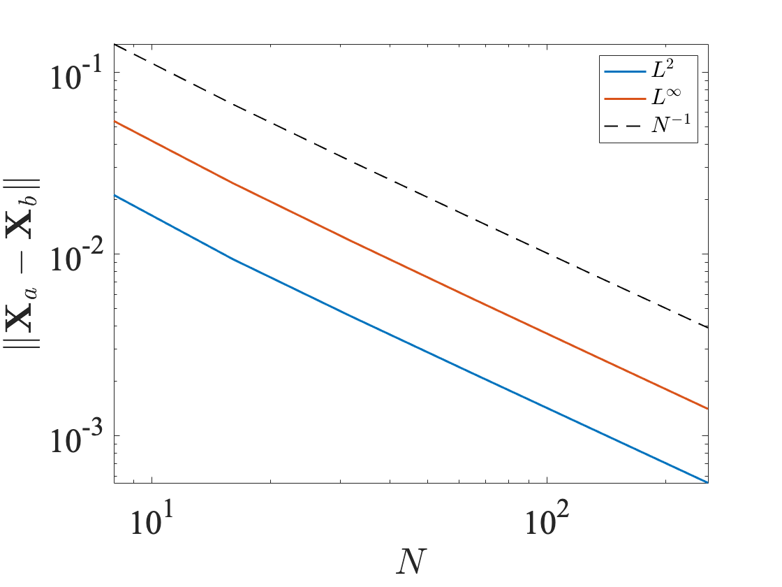
We next compare Methods (a) and (b) using the traveling wave forcing . The initial filament configuration is a straight line along the -axis. In Figure 9(a) we evolve the fiber until time and plot and as the number of fiber segments is increased. As in the setting, we observe convergence between the methods. In Figure 9(b), we again plot the actual positions (blue) and (red) for different snapshots in time.

Acknowledgments. Y.M. acknowledges support from the Math+X grant from the Simons Foundation and NSF DMS-2042144. L.O. acknowledges support from NSF Postdoctoral Fellowship DMS-2001959 and thanks Dallas Albritton for helpful discussion regarding the regularity theory of this problem.
References
- [1] S. Allende, C. Henry, and J. Bec. Stretching and buckling of small elastic fibers in turbulence. Physical review letters, 121(15):154501, 2018.
- [2] S. Camalet and F. Jülicher. Generic aspects of axonemal beating. New Journal of Physics, 2(1):24, 2000.
- [3] S. Camalet, F. Jülicher, and J. Prost. Self-organized beating and swimming of internally driven filaments. Physical review letters, 82(7):1590, 1999.
- [4] B. Chakrabarti, Y. Liu, O. Du Roure, A. Lindner, and D. Saintillan. Signatures of elastoviscous buckling in the dilute rheology of stiff polymers. Journal of Fluid Mechanics, 919, 2021.
- [5] R. Coy and H. Gadêlha. The counterbend dynamics of cross-linked filament bundles and flagella. Journal of The Royal Society Interface, 14(130):20170065, 2017.
- [6] O. Du Roure, A. Lindner, E. N. Nazockdast, and M. J. Shelley. Dynamics of flexible fibers in viscous flows and fluids. Annual Review of Fluid Mechanics, 51:539–572, 2019.
- [7] Y. El Alaoui-Faris, J.-B. Pomet, S. Régnier, and L. Giraldi. Optimal actuation of flagellar magnetic microswimmers. Physical Review E, 101(4):042604, 2020.
- [8] B. M. Friedrich, I. H. Riedel-Kruse, J. Howard, and F. Jülicher. High-precision tracking of sperm swimming fine structure provides strong test of resistive force theory. Journal of Experimental Biology, 213(8):1226–1234, 2010.
- [9] H. Gadêlha, E. Gaffney, D. Smith, and J. Kirkman-Brown. Nonlinear instability in flagellar dynamics: a novel modulation mechanism in sperm migration? Journal of The Royal Society Interface, 7(53):1689–1697, 2010.
- [10] H. Gadêlha and E. A. Gaffney. Flagellar ultrastructure suppresses buckling instabilities and enables mammalian sperm navigation in high-viscosity media. Journal of The Royal Society Interface, 16(152):20180668, 2019.
- [11] G. P. Galdi. On the self-propulsion of a rigid body in a viscous liquid by time-periodic boundary data. Journal of Mathematical Fluid Mechanics, 22(4):1–34, 2020.
- [12] G. P. Galdi and A. L. Silvestre. On the motion of a rigid body in a navier-stokes liquid under the action of a time-periodic force. Indiana University mathematics journal, pages 2805–2842, 2009.
- [13] F. Gancedo, R. Granero-Belinchón, and S. Scrobogna. Global existence in the lipschitz class for the n-peskin problem. arXiv preprint arXiv:2011.02294, 2020.
- [14] E. Garcia-Juarez, Y. Mori, and R. M. Strain. The peskin problem with viscosity contrast. arXiv preprint arXiv:2009.03360, 2020.
- [15] R. E. Goldstein and S. A. Langer. Nonlinear dynamics of stiff polymers. Physical review letters, 75(6):1094, 1995.
- [16] J. Gray and G. Hancock. The propulsion of sea-urchin spermatozoa. Journal of Experimental Biology, 32(4):802–814, 1955.
- [17] A. L. Hall-McNair, T. D. Montenegro-Johnson, H. Gadêlha, D. J. Smith, and M. T. Gallagher. Efficient implementation of elastohydrodynamics via integral operators. Physical Review Fluids, 4(11):113101, 2019.
- [18] A. Hilfinger, A. K. Chattopadhyay, and F. Jülicher. Nonlinear dynamics of cilia and flagella. Physical Review E, 79(5):051918, 2009.
- [19] M. Hines and J. Blum. Bend propagation in flagella. i. derivation of equations of motion and their simulation. Biophysical Journal, 23(1):41–57, 1978.
- [20] S. Hu, J. Zhang, and M. J. Shelley. Enhanced clamshell swimming with asymmetric beating at low reynolds number. Soft Matter, 2022.
- [21] R. Johnson and C. Brokaw. Flagellar hydrodynamics. a comparison between resistive-force theory and slender-body theory. Biophysical journal, 25(1):113–127, 1979.
- [22] J. B. Keller and S. Rubinow. Swimming of flagellated microorganisms. Biophysical Journal, 16(2):151–170, 1976.
- [23] L. Landau and E. Lifschitz. Theory of elasticity—course of theoretical physics, vol. 7 oxford. UK: Butterwoth-Heinemann, 1986.
- [24] E. Lauga. Floppy swimming: Viscous locomotion of actuated elastica. Physical Review E, 75(4):041916, 2007.
- [25] E. Lauga. The fluid dynamics of cell motility, volume 62. Cambridge University Press, 2020.
- [26] E. Lauga and C. Eloy. Shape of optimal active flagella. Journal of Fluid Mechanics, 730, 2013.
- [27] E. Lauga and T. R. Powers. The hydrodynamics of swimming microorganisms. Reports on Progress in Physics, 72(9):096601, 2009.
- [28] S. J. Lighthill. Mathematical biofluiddynamics. SIAM, 1975.
- [29] F.-H. Lin and J. Tong. Solvability of the stokes immersed boundary problem in two dimensions. Communications on Pure and Applied Mathematics, 72(1):159–226, 2019.
- [30] J. Liu, Y. Fu, X. Liu, and H. Ruan. Theoretical perspectives on natural and artificial micro-swimmers. Acta Mechanica Solida Sinica, 34(6):783–809, 2021.
- [31] J. S. Martín, J.-F. Scheid, T. Takahashi, and M. Tucsnak. An initial and boundary value problem modeling of fish-like swimming. Archive for rational mechanics and analysis, 188(3):429–455, 2008.
- [32] O. Maxian, A. Mogilner, and A. Donev. Integral-based spectral method for inextensible slender fibers in stokes flow. Physical Review Fluids, 6(1):014102, 2021.
- [33] O. Maxian, B. Sprinkle, C. S. Peskin, and A. Donev. The hydrodynamics of a twisting, bending, inextensible fiber in stokes flow. arXiv preprint arXiv:2201.04187, 2022.
- [34] T. Montenegro-Johnson, H. Gadelha, and D. J. Smith. Spermatozoa scattering by a microchannel feature: an elastohydrodynamic model. Royal Society Open Science, 2(3):140475, 2015.
- [35] C. Moreau, L. Giraldi, and H. Gadêlha. The asymptotic coarse-graining formulation of slender-rods, bio-filaments and flagella. Journal of the Royal Society Interface, 15(144):20180235, 2018.
- [36] Y. Mori and L. Ohm. An error bound for the slender body approximation of a thin, rigid fiber sedimenting in stokes flow. Research in the Mathematical Sciences, 7(2):1–27, 2020.
- [37] Y. Mori and L. Ohm. Accuracy of slender body theory in approximating force exerted by thin fiber on viscous fluid. Studies in Applied Mathematics, 2021.
- [38] Y. Mori, L. Ohm, and D. Spirn. Theoretical justification and error analysis for slender body theory. Communications on Pure and Applied Mathematics, 73(6):1245–1314, 2020.
- [39] Y. Mori, L. Ohm, and D. Spirn. Theoretical justification and error analysis for slender body theory with free ends. Archive for Rational Mechanics and Analysis, 235(3):1905–1978, 2020.
- [40] Y. Mori, A. Rodenberg, and D. Spirn. Well-posedness and global behavior of the peskin problem of an immersed elastic filament in stokes flow. Communications on Pure and Applied Mathematics, 72(5):887–980, 2019.
- [41] C. V. Neal, A. L. Hall-McNair, J. Kirkman-Brown, D. J. Smith, and M. T. Gallagher. Doing more with less: the flagellar end piece enhances the propulsive effectiveness of human spermatozoa. Physical Review Fluids, 5(7):073101, 2020.
- [42] Š. Nečasová, T. Takahashi, and M. Tucsnak. Weak solutions for the motion of a self-propelled deformable structure in a viscous incompressible fluid. Acta applicandae mathematicae, 116(3):329–352, 2011.
- [43] H. Nguyen and L. Fauci. Hydrodynamics of diatom chains and semiflexible fibres. Journal of The Royal Society Interface, 11(96):20140314, 2014.
- [44] L. Ohm. Remarks on regularized stokeslets in slender body theory. Fluids, 6(8):283, 2021.
- [45] O. Pironneau and D. Katz. Optimal swimming of flagellated micro-organisms. Journal of Fluid Mechanics, 66(2):391–415, 1974.
- [46] S. G. Pozveh, A. J. Bae, and A. Gholami. Resistive force theory and wave dynamics in swimming flagellar apparatus isolated from c. reinhardtii. Soft matter, 17(6):1601–1613, 2021.
- [47] A. Rahimian, S. K. Veerapaneni, and G. Biros. Dynamic simulation of locally inextensible vesicles suspended in an arbitrary two-dimensional domain, a boundary integral method. Journal of Computational Physics, 229(18):6466–6484, 2010.
- [48] I. H. Riedel-Kruse, A. Hilfinger, J. Howard, and F. Jülicher. How molecular motors shape the flagellar beat. HFSP journal, 1(3):192–208, 2007.
- [49] P. Sartori, V. F. Geyer, A. Scholich, F. Jülicher, and J. Howard. Dynamic curvature regulation accounts for the symmetric and asymmetric beats of chlamydomonas flagella. Elife, 5:e13258, 2016.
- [50] G. R. Sell and Y. You. Dynamics of evolutionary equations, volume 143. Springer, 2002.
- [51] S. E. Spagnolie and E. Lauga. The optimal elastic flagellum. Physics of Fluids, 22(3):455, 2010.
- [52] D. B. Stein, G. De Canio, E. Lauga, M. J. Shelley, and R. E. Goldstein. Swirling instability of the microtubule cytoskeleton. Physical review letters, 126(2):028103, 2021.
- [53] B. Thomases and R. D. Guy. The role of body flexibility in stroke enhancements for finite-length undulatory swimmers in viscoelastic fluids. Journal of Fluid Mechanics, 825:109–132, 2017.
- [54] J. Tong. Regularized stokes immersed boundary problems in two dimensions: Well-posedness, singular limit, and error estimates. Communications on Pure and Applied Mathematics, 74(2):366–449, 2021.
- [55] A.-K. Tornberg and M. J. Shelley. Simulating the dynamics and interactions of flexible fibers in stokes flows. Journal of Computational Physics, 196(1):8–40, 2004.
- [56] S. K. Veerapaneni, D. Gueyffier, D. Zorin, and G. Biros. A boundary integral method for simulating the dynamics of inextensible vesicles suspended in a viscous fluid in 2d. Journal of Computational Physics, 228(7):2334–2353, 2009.
- [57] S. K. Veerapaneni, A. Rahimian, G. Biros, and D. Zorin. A fast algorithm for simulating vesicle flows in three dimensions. Journal of Computational Physics, 230(14):5610–5634, 2011.
- [58] B. J. Walker and E. A. Gaffney. Regularised non-uniform segments and efficient no-slip elastohydrodynamics. Journal of Fluid Mechanics, 915, 2021.
- [59] B. J. Walker, K. Ishimoto, and E. A. Gaffney. Efficient simulation of filament elastohydrodynamics in three dimensions. Physical Review Fluids, 5(12):123103, 2020.
- [60] R. Waszkiewicz, P. Szymczak, and M. Lisicki. Stability of sedimenting flexible loops. Journal of Fluid Mechanics, 919, 2021.
- [61] C. H. Wiggins and R. E. Goldstein. Flexive and propulsive dynamics of elastica at low reynolds number. Physical Review Letters, 80(17):3879, 1998.
- [62] C. H. Wiggins, D. Riveline, A. Ott, and R. E. Goldstein. Trapping and wiggling: elastohydrodynamics of driven microfilaments. Biophysical Journal, 74(2):1043–1060, 1998.
- [63] Y.-N. Young, M. Downs, and C. R. Jacobs. Dynamics of the primary cilium in shear flow. Biophysical journal, 103(4):629–639, 2012.
- [64] T. S. Yu, E. Lauga, and A. Hosoi. Experimental investigations of elastic tail propulsion at low reynolds number. Physics of Fluids, 18(9):091701, 2006.