\acmVolume\acmNumber\acmArticle

arXiv \acmYear \acmMonth

{bottomstuff}

Author’s addresses:

E. Bertolazzi, Dipartimento di Ingegneria Industriale, Università degli Studi di Trento, Via Sommarive 9, Trento (ITaly) email:enrico.bertolazzi@unitn.it

and

A. Falini, Dipartimento di Informatica, Università degli Studi di Bari Aldo Moro, Via Orabona 4, 70125 Bari (Italy). email:antonella.falini@uniba.it

and

F. Mazzia, Dipartimento di Informatica, Università degli Studi di Bari Aldo Moro, Via Orabona 4, 70125 Bari (Italy). email:francesca.mazzia@uniba.it

The Object Oriented C++ library QIBSH++ for Hermite spline Quasi Interpolation

ENRICO BERTOLAZZI ANTONELLA FALINI FRANCESCA MAZZIA Affiliation: Dipartimento di Ingegneria Industriale Università degli Studi di Trento. Affiliation: Dipartimento di Informatica, Università degli Studi di Bari Aldo Moro, Italy. Affiliation: Dipartimento di Informatica, Università degli Studi di Bari Aldo Moro, Italy.

Abstract

The library QIBSH++ is a C++ object oriented library for the solution of Quasi Interpolation problems. The library is based on a Hermite Quasi Interpolating operator, which was derived as continuous extensions of linear multistep methods applied for the numerical solution of Boundary Value Problems for Ordinary Differential Equations. The library includes the possibility to use Hermite data or to apply a finite difference scheme for derivative approximations, when derivative values are not directly available. The generalization of the quasi interpolation procedure to surfaces and volumes approximation by means of a tensor product technique is also implemented. The method has been also generalized for one dimensional vectorial data, periodic data, and for two dimensional data in cylindrical coordinates, periodic with respect to the angular argument. Numerical tests show that the library could be used efficiently in many practical problems.

Keywords:

Algorithms, Theory, Design

keywords

Quasi Interpolation, B-splines

1 Introduction

There has been a lot of study in constructing good software for interpolation and data fitting using spline. The first package pppack of de Boor, was available in Netlib from 1992 but the first release was dated 1971 [de Boor, 1972, de Boor, 2001]. The Matlab package for spline interpolation and fitting data is based on the de Boor subroutines. Later on in 1973, the algorithm numbered 461, was published on ACM Transaction of mathematical software and it was related to he computation of a cubic spline approximation to the solution of a linear second order boundary value ordinary differential equations [Burkowski and Hoskins, 1973]. The same journal published in 2016 a B-spline Adaptive Collocation software for PDEs with Interpolation-Based Spatial Error Control [Pew et al., 2016]. Both algorithms use spline functions for the solution of differential problems with collocation. In 1993 the tspack package for tension spline curve-fitting package [Renka, 1993] and in 2009 its extension for curve design and data fitting [Renka, 2009] have been published. Nowadays, a lot of wrappers or re-implementations of the pppack library are available in different languages like C, C++, Python, Matlab. Other functions for scattered data are available. We recall the Fortran package fitpack of Paul Dierks available in Netlib [Dierckx, 1993] and the C package TSFIT for two-stage scattered data fitting [Davydov and Zeilfelder, 2005]; the C++ library G+SMO [Jüttler et al., 2014, Mantzaflaris, 2019] and the GeoPDEs package [De Falco et al., 2011, Vázquez, 2016], both for iso-geometric analysis. Other libraries and software’s available for spline fitting and geometric spline constructions are [Elber, 1990, Schumaker, 2018, Grimstad et al., 2015, Walker et al., 2019] .

The library we present here is based on the so called Hermite BS quasi-interpolant (BSH QI in short) introduced in [Mazzia and Sestini, 2009a], derived from a class of linear multistep boundary value methods based on spline collocation [Mazzia et al., 2006a].

Univariate spline Quasi Interpolants (QIs) are operators for function approximations with the following form:

Q_{d}\left(f\right)=\sum_{j\in J}{\mu_{j}(f)B_{j}},

(1)

where $\left\{B_{j},j\in J\right\}$ is the B-spline basis of a given degree $d$ , and $\mu_{j}(f)$ are local linear functionals. One of the main properties of QIs is that the coefficients $\mu_{j}(f)$ depend locally on the data, making them competitive with respect to global approximation methods.

The library QIBSH++ is an object oriented extension of the C library QIBSH presented in [Iurino and Mazzia, 2013], [Iurino, 2014] and includes all the procedures for the BSH Quasi Interpolation scheme, a generalization of the former to be used when derivative values are not available, and an extension of the BSH QI operator to bivariate and trivariate functions, which uses a suitable tensor product technique. Moreover, Matlab and Octave interfaces have been implemented for all the objects, in order to make them available in this well known numerical computing environment. This is an important feature, since some of the procedures in QIBSH++ will be also part of the Matlab code TOM for the numerical solution of Boundary Value Problem for Ordinary Differential Equations [Mazzia et al., 2006b, Mazzia et al., 2006c, Mazzia et al., 2009a].

The aim of this library is to make available to a wider audience quasi-interpolation procedures that could be useful when interpolation is not necessary and the error in the data is negligible. In many applications, moreover, the first derivative is a known data and so Hermite quasi-interpolation could give more accurate results than standard quasi-interpolation. We experienced a lack of general purpose codes based on high order quasi-interpolation, especially for two and three dimensional data and in many applications where is required in output continuity for higher derivatives and for which codes that are based on radial basis functions, or bi-variate splines are not suited.

In Section 2 we give a brief description of the BSH QI in one dimension, introducing also the approximated BSH, where derivative values are not directly used in the operator, but derived using suitable finite difference schemes. In Section 3 the BSH Quasi Interpolant is extended to the approximation of tensor product surfaces and volumes. In Section 4 we describe the implementation details of the algorithm. Finally, in Section 5 we provide some numerical examples giving an idea of the performance of the QIBSH++ library. The behavior of QIBSH++ is compared to the QI method [Sablonnière, 2005], and QI linear, both implemented by the authors and to the spline interpolation routines from Matlab, on standard test functions from the literature. We also show how to improve the time efficiency of the TOM code for BVP problems using the QIBSH++ library. Moreover, a surface parameterization with high smoothness for complex geometries is presented in subsection 5.4. We conclude the work showing that the QIBSH++ library can be applied for the solution of two real data problems: a continuous digital elevation model and a biomedical application.

2 BSH Quasi Interpolants in One Dimension

Differential quasi interpolants (DQI) [de Boor, 1976, de Boor, 2001] are linear approximating operators where the coefficients of the approximating splines are computed by linear combinations or averages of derivative values of $f$ , a continuous function defined on an interval $[a,b]$ . The idea of applying a Hermite Quasi Interpolating technique to our problem comes from a different area, since BS methods are a class of Boundary Value Methods for ODEs [Brugnano and Trigiante, 1998, Mazzia et al., 2006b]. Using this class of BS methods it is possible to determine a spline $s=\sum_{i\in I}c_{i}B_{i}$ on the mesh defined by the knot vector $\pi=[x_{0},\ldots,x_{N}]$ , where $a=x_{0}<x_{1}<\ldots<x_{N}=b$ , satisfying the Hermite interpolation conditions $s(x_{i})=f_{i}$ , $s^{\prime}(x_{i})=f^{\prime}_{i}$ for all $i=0,\ldots,N$ , where $f_{0},\ldots,f_{N}$ and $f^{\prime}_{0},\ldots,f^{\prime}_{N}$ are respectively the values of the function $f$ and of the first derivative $f^{\prime}$ and both, $f_{i},f^{\prime}_{i}\in{\mathbb{R}}^{p}\;\forall i$ , with $p>1$ for the multidimensional case.

Here, the set $\left\{B_{i}:\;i\in I\right\}$ is the B-spline basis for the space $S_{d,\pi}$ of $d$ -degree splines on the knots $\pi$ . The BS Hermite Quasi Interpolation scheme approximates a function $f$ on an interval $\left[a,b\right]$ starting from its values, and from those of the first derivative on $N+1$ mesh points $\pi$ . We want an approximating function in the space $S_{d,\pi}$ of the splines of degree $d$ with knots $\pi$ . Usually, we work with an extended knot set considering a total of $2d$ additional boundary knots. The new knot set is then defined as $\bm{\tau}=\{\tau_{i}\}_{i=1}^{N_{\tau}}=\left\{x_{-d},\ldots,x_{-1},x_{0},\ldots,x_{N},x_{N+1},\ldots,x_{N+d}\right\}$ , where $N_{\tau}=N+2d+1$ . The auxiliary boundary knots are commonly chosen equal to the ending points of the interval. The Quasi Interpolating spline is then:

Q^{\left(BS\right)}_{d}\left(f\right)=\sum_{j=-d}^{N-1}{\mu^{\left(BS\right)}_{j}(f)B_{j}},

(2)

with the coefficients $\mu_{j}^{(BS)}(f)$ expressed by

\mu^{(BS)}_{j}(f)=\displaystyle\sum_{i=1}^{d}\begin{cases}\hat{\alpha_{i}}^{(-1,j+d+1)}f_{i-1}-h_{k_{1}}\hat{\beta_{i}}^{(-1,j+d+1)}f^{\prime}_{i-1}&j=-d,\ldots,-2,\\[10.00002pt] \hat{\alpha_{i}}^{(j,d)}f_{i+j}-h_{j+k_{1}+1}\hat{\beta_{i}}^{(j,d)}f^{\prime}_{i+j}&j=-1,\ldots,\tilde{N},\\[10.00002pt] \hat{\alpha_{i}}^{(\tilde{N},j+d-\tilde{N})}f_{\tilde{N}+i}-h_{N-k_{2}}\hat{\beta_{i}}^{(\tilde{N},j+d-\tilde{N})}f^{\prime}_{\tilde{N}+i}&j=\tilde{N}+1,\ldots,N-1,\end{cases}

(3)

where $\tilde{N}=N-d$ , $\bm{\hat{\alpha}}^{(j,r)}=\left(\hat{\alpha}^{(j,r)}_{1},\ldots,\hat{\alpha}^{(j,r)}_{d}\right)^{T}$ and $\bm{\hat{\beta}}^{(j,r)}=\left(\hat{\beta}^{(j,r)}_{1},\ldots,\hat{\beta}^{(j,r)}_{d}\right)^{T}$ are solutions of local linear systems of size $2d\times 2d$ , whose coefficient matrix depends on the values of the B-splines $B_{i}$ (see [Mazzia et al., 2006b]). The functionals $\mu_{j}^{(BS)}(f)$ in (2) depend locally on the values $(f_{i},f^{\prime}_{i}),\,i=0,\ldots,N$ , where $f_{i}$ and $f^{\prime}_{i}$ denote the exact function and first derivative values, respectively. Following the notation used in [Mazzia and Sestini, 2012], we write the coefficients in the form:

\bm{\mu}^{(BS)}=(\hat{A}\otimes I_{p})\mathbf{f}-(\hat{H}\hat{B}\otimes I_{p})\mathbf{f}^{\prime},

(4)

where $\hat{A}$ and $\hat{B}$ are banded matrices in ${\mathbb{R}}^{N+d\times N+1}$ containing the local coefficients $\bm{\hat{\alpha}}^{(j,r)}$ and $\bm{\hat{\beta}}^{(j,r)}$ , while $\hat{H}=\mathrm{diag}(\hat{h}_{1},\ldots,\hat{h}_{N+d})$ , with

\hat{h}_{i}=\begin{cases}{h}_{k_{1}},\quad&\text{if}~~i\leq d\\ {h}_{k_{1}+i-d},\quad&\text{if}~~d+1\leq i\leq N\\ {h}_{N-k_{2}},\quad&\text{if}~~i\geq N+1,\end{cases}

(5)

and $\mathbf{f}=\left(f_{0}^{\top},\ldots,f_{N}^{\top}\right)^{\top}$ , $\mathbf{f}^{\prime}=({f^{\prime}_{0}}^{\top},\ldots,{f^{\prime}_{N}}^{\top})^{\top}$ , and $I_{p}$ is the identity operator of dimension $p$ .

The coefficient determination of the Quasi Interpolant $Q^{(BS)}_{d}(f)$ in the B-spline representation, requires the solution of local linear systems for $j=-1,\>r=1,\ldots,d$ , for $0\leq j\leq N-d-1,\>r=d$ , and for $j=N-d,\>r=d,\ldots,2d-1$ . The computational cost is the one for solving $N+d$ linear systems of dimension $2d\times 2d$ . They are solved by the efficient and stable algorithm presented in [Mazzia et al., 2006c]. When low degree polynomials are used, we can give explicit expressions of the coefficient vectors. Note that for a uniform knot mesh $\pi$ , the inner coefficient vectors $\bm{\hat{\alpha}}^{(j,d)}$ and $\bm{\hat{\beta}}^{(j,d)}$ , for $j=-1,\ldots,N-d$ do not depend on $j$ , so the expressions of coefficients $\mu^{(BS)}_{j}(f)$ may be derived beforehand.

The Quasi Interpolation procedure described so far is of Hermite type, since it depends on the function and its first derivative values. Often in applications, we do not have such information, and only approximate values of $f$ and $f^{\prime}$ are available. In some cases, we may be given only the values of the function at mesh knots, and in order to construct the QI we must use approximate values for the first derivatives. For this reason, we combine the Quasi Interpolation scheme with a symmetric finite difference scheme approximating the derivatives of $f$ at the mesh points. In order to distinguish it from the original one, we refer to the original BSH as $Q_{d}^{(BS)}$ , and to the one using approximate values of $f^{\prime}$ , as $Q^{(BSa)}_{d}$ .

Indeed, we can approximate the first derivative values of a sufficiently smooth function $f$ on a grid $x_{0}<\ldots<x_{N}$ , using the $l$ -step finite difference scheme used in [Mazzia and Sestini, 2012]. So we have the following scheme:

\begin{cases}\displaystyle\sum_{i=0}^{l}\gamma_{i}^{(n)}f_{i}=f^{\prime}(x_{n})+\mathcal{O}(h^{l}),\quad&n=0,\ldots,l_{1}-1,\\ \displaystyle\sum_{i=0}^{l}\gamma_{i}^{(n)}f_{n-l_{1}+i}=f^{\prime}(x_{n})+\mathcal{O}(h^{l}),\quad&n=l_{1},\ldots,N-l_{2},\\ \displaystyle\sum_{i=0}^{l}\gamma_{i}^{(n)}f_{N-l+i}=f^{\prime}(x_{n})+\mathcal{O}(h^{l}),\quad&n=N-l_{2}+1,\ldots,N,\end{cases}

(6)

where $l_{1}=\lfloor{l/2}\rfloor$ , $l_{2}=l-l_{1}$ , $h_{i}=x_{i}-x_{i-1}$ , $i=1,\ldots,N$ , and $h=\max_{1\leq i\leq N}h_{i}$ . The coefficients $\gamma_{i}^{(n)}$ are computed imposing that the local truncation error of the resulting method is $\mathcal{O}(h^{l})$ . The derivative approximation scheme is modified in order to have a symmetric global approximation when the mesh is symmetric. It can be written as

(\Gamma^{(l)}\otimes I_{p})\begin{pmatrix}f(x_{0})\\ \vdots\\ f(x_{N})\end{pmatrix}=\begin{pmatrix}f^{\prime}(x_{0})\\ \vdots\\ f^{\prime}(x_{N})\end{pmatrix}+\mathcal{O}(h^{l}),

(7)

where the banded matrix $\Gamma^{(l)}\in{\mathbb{R}}^{(N+1)\times(N+1)}$ has the following structure:

\Gamma^{(l)}=\begin{pmatrix}\gamma_{0}^{(0)}&\cdots&\gamma_{l}^{(0)}&0&\cdots&\cdots&0\\ \vdots&&\vdots&\vdots&&&\vdots\\ \gamma_{0}^{(l_{1}-1)}&\cdots&\gamma_{l}^{(l_{1}-1)}&0&&&\vdots\\ 0&\ddots&&\ddots&\ddots&&\vdots\\ \vdots&\ddots&\gamma_{0}^{(j)}&\cdots&\gamma_{l}^{(j)}&\ddots&\vdots\\ \vdots&&\ddots&\ddots&&\ddots&0\\ \vdots&&&0&\gamma_{0}^{(N-l_{2}+1)}&\cdots&\gamma_{l}^{(N-l_{2}+1)}\\ \vdots&&&\vdots&\vdots&&\vdots\\ 0&\cdots&\cdots&0&\gamma_{0}^{(N)}&\cdots&\gamma_{l}^{(N)}\end{pmatrix}.

(8)

The first derivative approximation on the mesh points is $\mathbf{\tilde{f}^{\prime}}=(\Gamma^{(l)}\otimes I_{p})\mathbf{f}$ . Combining this scheme with the BSH formula for the QI coefficients we get the Quasi Interpolant:

Q^{\left(BSa\right)}_{d}\left(f\right)=\sum_{j=-d}^{N-1}{\tilde{\mu}^{\left(BSa\right)}_{j}(f)B_{j}},

(9)

It can be proven that the following error bound holds:

\|f-Q^{(BSa)}_{d}(f)\|_{\infty}\leq Lh^{d+1}\|D^{d+1}f\|_{\infty}+\tilde{L}\,h^{l+1},

(10)

where $L$ and $\tilde{L}$ depends on the spline degree $d$ , on the smoothness of $f$ and on the geometric properties, like quasi-uniformity, of the underlying knot mesh. For more details we refer to [Falini et al., 2022]. Note that a similar error bound holds also for the operator $Q_{d}^{(BS)}$ , see [Mazzia and Sestini, 2009b] for the details.

3 BSH Quasi Interpolants and Tensor Product

The general tensor product framework can be used with the BSH QI from the previous section. Applying the one dimensional operators either first along the x-direction and then the y-direction, or vice-versa, we compute the approximating surface. Suppose we are given a function $f:{\mathbb{R}}^{2}\rightarrow{\mathbb{R}}$ $f=f(x,y)$ defined on a rectangular planar domain $R=\left[a,b\right]\times\left[c,d\right]$ . We choose the spline degrees to be $d_{x}$ and $d_{y}$ and select $m_{1}=N+1$ and $m_{2}=M+1$ knots respectively on $x$ and $y$ directions. Consider the partitions with the additional boundary knots defined as:

\begin{array}[]{l}\tau_{x}=x_{-d_{x}}\leq\cdots\leq x_{0}=a<\cdots x_{i}\cdots<b=x_{N}\leq x_{N+1}\leq\cdots\leq x_{N+d_{x}},\\[10.00002pt] \tau_{y}=y_{-d_{y}}\leq\cdots\leq y_{0}=c<\cdots y_{j}\cdots<d=y_{M}\leq y_{M+1}\leq\cdots\leq y_{M+d_{y}}.\end{array}

(11)

We denote the extended knot vectors as $\bm{\tau}_{x}$ and $\bm{\tau}_{y}$ , with sizes respectively $N_{\tau_{x}}$ and $N_{\tau_{y}}$ . The dimension of the spline spaces are $n_{1}=N+d_{x}$ and $n_{2}=M+d_{y}$ respectively for each knot partition. Any spline $s$ in the tensor product space is written in the form:

s(x,y)=\sum^{n_{1}}_{p=1}\sum^{n_{2}}_{q=1}c_{pq}\phi_{p}(x)\psi_{q}(y)\quad\forall(x,y)\in{\mathbb{R}}^{2},

(12)

where $\phi_{p}$ and $\psi_{q}$ are the B-splines elements. Also, the exact values of the function $f$ and of its partial derivatives $f_{x}$ , $f_{y}$ and $f_{xy}$ are assigned on the grid points given in matrix form respectively as $\mathbf{F}=(f)_{i,j}$ , $\mathbf{F}_{x}=(f_{x})_{i,j}$ , $\mathbf{F}_{y}=(f_{y})_{i,j}$ , and $\mathbf{F}_{xy}=(f_{xy})_{i,j}\in{\mathbb{R}}^{m_{1}\times m_{2}}$ , where $f_{i,j}=f(x_{i},y_{j})$ for all indices. The aim is to find a function $g=g(x,y)$ in the tensor product space (12) aproximating $f$ , finding the coefficient matrix $\mathbf{C}=(c_{pq})\in{\mathbb{R}}^{n_{1}\times n_{2}}$ . The tensor product technique applied to the BSH follows a very simple idea: the grid is divided into knot lines according to its knot partitions, and a specific number of one dimensional QI problems is solved along the two directions.

The coefficients of the spline function $s(x,y)$ are computed using the QI BSH tensor product algorithm, which is summarized by the following steps.

{longenum}

For each $j=1,...,m_{2}$ , pick up the function and the $x$ partial derivatives of the $j$ -th line in the grid, and use them applying the one dimensional BSH $Q_{d_{x}}^{(BS)}$ . Solve $m_{2}$ one dimensional QI problems, storing the resulting coefficients into the matrix $\mathbf{D}=(d_{pj})\in{\mathbb{R}}^{n_{1}\times m_{2}}$ .

In matrix formulation we have

\mathbf{D}=\hat{A}_{x}\mathbf{F}-\hat{H}_{x}\hat{B}_{x}\mathbf{F}_{x},

(13)

where the subscript in the matrices $\hat{A}_{x}$ , $\hat{B}_{x}$ and $\hat{H}_{x}$ , specifies the equation (4) for the local coefficients on the $x$ -direction with $p=1$ .

For each $j=1,...,m_{2}$ , pick up the $y$ and the mixed $xy$ partial derivatives of the function $f$ on the $j$ -th line in the grid, and apply the one dimensional operator $Q_{d_{x}}^{(BS)}$ . As in the previous step, $m_{2}$ one dimensional QI problems are solved, saving the coefficients into $\mathbf{D^{\prime}}=(d^{\prime}_{pj})\in{\mathbb{R}}^{n_{1}\times m_{2}}$ . In matrix formulation:

\mathbf{D^{\prime}}=\hat{A}_{x}\mathbf{F}_{y}-\hat{H}_{x}\hat{B}_{x}\mathbf{F}_{xy}.

(14)

Now, simply switch the direction, and consider the quasi interpolant operator $Q_{d_{y}}^{(BS)}$ along the $y$ direction. For each $p=1,\ldots,n_{1}$ pick up the values in the $p$ -th rows of the matrices $\mathbf{D}=(d_{p,j})$ and $\mathbf{D^{\prime}}=(d^{\prime}_{p,j})$ , and apply to these values the one dimensional BSH $Q_{d_{y}}^{(BS)}$ . So, after solving $n_{1}$ one dimensional QI problems in the $y$ direction, the matrix $\mathbf{C}=(c_{p,q})$ containing the coefficients of the tensor product form (12) is built. Note that in this last step we are using the BSH quasi interpolating scheme $Q_{d_{y}}^{(BS)}$ on the $y$ -direction, replacing the function and derivative values by the elements from the matrices $\mathbf{D}$ and $\mathbf{D}^{\prime}$ , namely in matrix form:

\mathbf{C}=\mathbf{D}\hat{A}^{T}_{y}-\mathbf{D^{\prime}}(\hat{H}_{y}\hat{B}_{y})^{T}=\left(\hat{A}_{x}\mathbf{F}-\hat{H}_{x}\hat{B}_{x}\mathbf{F}_{x}\right)\hat{A}^{T}_{y}-\left(\hat{A}_{x}\mathbf{F}_{y}-\hat{H}_{x}\hat{B}_{x}\mathbf{F}_{xy}\right)\left(\hat{H}_{y}\hat{B}_{y}\right)^{T}.

(15)

When only function values are available, approximations for partial derivatives in both directions are computed using the scheme (7), that is

\mathbf{F}_{x}\approx\Gamma^{(l_{x})}_{x}\mathbf{F},\quad\mathbf{F}_{y}\approx\mathbf{F}(\Gamma^{(l_{y})}_{y})^{T},\quad\mathbf{F}_{xy}\approx\mathbf{F}_{x}(\Gamma^{(l_{y})}_{y})^{T}\approx\Gamma^{(l_{x})}_{x}\mathbf{F}_{y}\approx\Gamma^{(l)}_{x}\mathbf{F}(\Gamma^{(l_{y})}_{y})^{T}.

(16)

Matrix expressions (13) and (14) from the tensor product scheme are now

\mathbf{D}^{(a)}=\hat{A}_{x}\mathbf{F}-\hat{H}_{x}\hat{B}_{x}\Gamma^{(l_{x})}_{x}\mathbf{F},\quad\text{ and }\quad\mathbf{D^{\prime}}^{(a)}=\hat{A}_{x}\mathbf{F}(\Gamma^{(l_{y})}_{y})^{T}-\hat{H}_{x}\hat{B}_{x}\Gamma^{(l_{y})}_{x}\mathbf{F}(\Gamma^{(l_{y})}_{y})^{T},

(17)

and they satisfy

\mathbf{D^{\prime}}^{(a)}=\mathbf{D}^{(a)}(\Gamma^{(l_{y})}_{y})^{T}.

(18)

This proves it is theoretically equivalent, to compute the approximation of partial derivatives starting from $\mathbf{F}$ , and then apply the tensor product of BSH QI, or apply the finite difference scheme to the elements in $\mathbf{D}^{(a)}$ . The latter way has been used in our library implementation, since it reduces the computational cost. The coefficients matrix of the representation (12) is obtained in this case as

\mathbf{C}^{(a)}=(\hat{A}_{x}-\hat{H}_{x}\hat{B}_{x}\Gamma^{(l_{x})}_{x})\mathbf{F}\hat{A}_{y}^{T}-(\hat{A}_{x}-\hat{H}_{x}\hat{B}_{x}\Gamma^{(l)}_{x})\mathbf{F}(\Gamma^{(l_{y})}_{y})^{T}(\hat{H}_{y}\hat{B}_{y})^{T},

(19)

or, in a more compact form:

\mathbf{C}^{(a)}=(\hat{A}_{x}-\hat{H}_{x}\hat{B}_{x}\Gamma^{(l_{x})}_{x})\mathbf{F}(\hat{A}_{y}-\hat{H}_{y}\hat{B}_{y}\Gamma^{(l_{y})}_{y})^{T}.

(20)

In the following, we address the extension of the operator $Q_{d}^{(BSa)}$ to the approximation of a three valued function $f=f(x,y,z)$ , with $f:{\mathbb{R}}^{3}\rightarrow{\mathbb{R}}$ defined on a domain $R=\left[a_{x},b_{x}\right]\times\left[a_{y},b_{y}\right]\times\left[a_{z},b_{z}\right]$ .

Consider the partitions with the additional boundary knots defined as:

\begin{array}[]{l}\tau_{x}=x_{-d_{x}}\leq\ldots\leq x_{0}=a_{x}<\ldots x_{i}\ldots<b_{x}=x_{N_{x}}\leq x_{N_{x}+1}\leq\ldots\leq x_{N_{x}+d_{x}},\\[10.00002pt] \tau_{y}=y_{-d_{y}}\leq\ldots\leq y_{0}=a_{y}<\ldots y_{j}\ldots<b_{y}=y_{N_{y}}\leq y_{N_{y}+1}\leq\ldots\leq y_{N_{y}+d_{y}}.\\[10.00002pt] \tau_{z}=z_{-d_{z}}\leq\ldots\leq z_{0}=a_{z}<\ldots z_{j}\ldots<b_{z}=z_{N_{z}}\leq z_{N_{z}+1}\leq\ldots\leq z_{N_{z}+d_{z}}.\end{array}

(21)

To explain better the application of the quasi-interpolant on a multi dimensional space it is convenient to express the data using a three dimensional tensor

\mathcal{F}\in{\mathbb{R}}^{Nx\times Ny\times Nz},\qquad\mathit{f}_{ijk}=f(x_{i},y_{j},z_{k})

and the coefficients of the spline using $n$ -mode product between a tensor $\mathcal{X}\in{\mathbb{R}}^{I_{1}\times I_{2}\times I_{3}}$ and a matrix $A\in{\mathbb{R}}^{n\times I_{j}}$ as defined in [Kolda and Bader, 2009]:

\mathcal{Y}=\mathcal{X}\times_{j}A\Leftrightarrow Y_{j}=AX_{j}

where $Y_{j},X_{j}$ are the mode- $j$ unfolding of ${\cal Y}$ and ${\cal X}$ .

Here we report only the version of the quasi-interpolant using approximate derivative, because it is less expensive from a computational point of view. The coefficient of the approximated BSH QI version can been in fact calculated, like for the bi-dimensional case, by applying the one dimensional quasi-interpolant along the three directions. We obtain that:

\mathcal{C}^{(a)}=\mathcal{F}\times_{1}(\hat{A}_{x}-\hat{H}_{x}\hat{B}_{x}\Gamma^{(l_{x})}_{x})\times_{2}(\hat{A}_{y}-\hat{H}_{y}\hat{B}_{y}\Gamma^{(l_{y})}_{y})^{T}\times_{3}(\hat{A}_{z}-\hat{H}_{z}\hat{B}_{z}\Gamma^{(l_{z})}_{z})^{T}.

(22)

Additional details can be found in [Falini et al., 2022].

Remark 3.1

Note that by using the $n$ -mode product we can express the coefficient matrix of equation (20) as,

\displaystyle C^{(a)}={\cal F}\times_{1}(\hat{A}_{x}-\hat{H}_{x}\hat{B}_{x}\Gamma^{(l_{x})}_{x})\times_{2}(\hat{A}_{y}-\hat{H}_{y}\hat{B}_{y}\Gamma^{(l_{y})}_{y})^{T}.

With this operation also the generalization to any dimension can be easily derived.

4 Implementation Details

The library QIBSH++ is a collection of C++ procedures managing the Hermite Quasi Interpolation for functions of one (scalar and vectorial functions), two and three variables. A Matlab toolbox is also available, that allow to handle all the procedure in Matlab.

This library is an improved version of the C version of QIBSH library described in [Iurino, 2014, Iurino and Mazzia, 2013]. The new implementation use more efficiently memory and dynamic memory usage. The C++ classes are mapped in Matlab classes using MEX interfacing mechanism. In practice each Matlab class instance store a pointer to the corresponding C++ class instance and each method for the Matlab class call a method of the corresponding C++ class.

This approach permits to develop and test algorithm using QIBSH in Matlab. This remapping introduce an overhead that is small and acceptable for the proposed applications. In any case, for best performance it is easy to translate to Matlab to C++.

4.1 C++ classes

The library is organized as a set of classes that interact together for the Quasi interpolant build and evaluation.

•
B-spline basis computation
- –
  
  Bspline
  This class implement the classical B-spline as described in [de Boor, 2001, Schumaker, 2007]. Recurrence formula for derivative and integral, standard knot placements, tensor product B-spline evaluation given the support polygon.
•
Finite Difference
- –
  
  FiniteDifferenceUniformD1
- –
  
  FiniteDifferenceD1
  This two classes implement the finite difference approximation of derivative given a list $(x_{i},y_{i})$ of interpolation points. The class FiniteDifferenceUniformD1 do the same computation more efficiently when coordinated $x_{i}$ are uniformly distributed.
•
Derivative approximation
- –
  
  ApproximateDerivative
- –
  
  ApproximateDerivative2D
  This classes uses FiniteDifferenceUniformD1 and FiniteDifferenceD1 to build the finite difference approximation of a set of one dimensional $(x_{i},y_{i})$ or two dimensional $(x_{ij},y_{ij},z_{ij})$ function sampling. In 2D cases mixed derivatives are obtained by applying finite difference in the $y$ direction to the approximate $x$ derivative. The classes manages cyclic data approximation if required.
•
Quasi Hermite 1D
- –
  
  QuasiHermite
- –
  
  QuasiHermiteApprox
  The classes compute the B-spline polygon corresponding to the QIBSH approximation. The first class uses points and analytical derivative at the corresponding points. The second class approximate the derivative using finite difference from class ApproximateDerivative.+
•
Quasi Hermite 2D
- –
  
  QuasiHermite2D
  This is the base class that compute the polygon for the B-spline that correspond to the QIBSH approximation of 2D surface data. The 2D points are passed to the class with $x$ , $y$ and mixed $xy$ derivatives at the points.
- –
  
  QuasiHermite2Dapprox
  This class is derived from QuasiHermite2D and compute the polygon for the B-spline that correspond to the QIBSH approximation of 2D surface data. The derivative respect to $x$ , $y$ and mixed $xy$ needed for base class are approximated using finite difference with class ApproximateDerivative2D.
- –
  
  QuasiHermite2Dsurface
  This class is derived from QuasiHermite2D. In addition the class store the computed B-spline polygon so that can be evaluated at any points without the requirement to pass the B-spline polygon.
- –
  
  QuasiHermite2DapproxSurface
  This class is derived from QuasiHermite2Dapprox. In addition the class store the computed B-spline polygon so that can be evaluated at any points without the requirement to pass the B-spline polygon.

4.2 Matlab classes

QIBSH++ library is connected with Matlab using MEX interface. The mapping is not one to one but is a little bit of higher level.

•
B-spline basis computation
- –
  
  Bspline
  This is a one-to-one remap of the corresponding C++ class.
- –
  
  Bspline1D
  This Matlab class remap the C++ class QuasiHermite and QuasiHermiteApprox. It stores in the Matlab class data the B-spline polygon and can use analytical derivative or use finite difference approximation.
•
Approximation of derivatives using finite difference
- –
  
  ApproximateDerivative1D
- –
  
  ApproximateDerivative2D
  This is a one-to-one remap of the corresponding C++ class.
•
Spline build using quasi interpolation
- –
  
  QIBSH1D
- –
  
  QIBSH2D
  This are high level remaps of the C++ classes QuasiHermite, QuasiHermiteApprox, QuasiHermite2D, QuasiHermiteApprox2D with the storage in the Matlab class of the resulting B-spline polygon.

The Matlab usage of the QIBSH library is particularly simple:

⬇

1 % Instantiate in Q a MATLAB class for 1D Quasi Interpolant

2 Q = QIBSH1D(’Qhermite’);

3 % Build a quasi interpolant

4 % d = degree of the interpolant

5 % (x(i),y(i)) = quasi interpolation points

6 % yprime(i) = derivative at the quasi interpolation point

7 % fifth argument if true build a periodic quasi interpolant

8 Q.build( d, x, y, yprime, false );

after build is easy to compute points and derivative on the B-spline:

⬇

1 % Evaluate y = Q(x)

2 y = Q.eval(x);

3 % Evaluate y = Q’(x)

4 Dy = Q.eval(x,1);

5 % Evaluate y = Q”(x)

6 DDy = Q.eval(x,2);

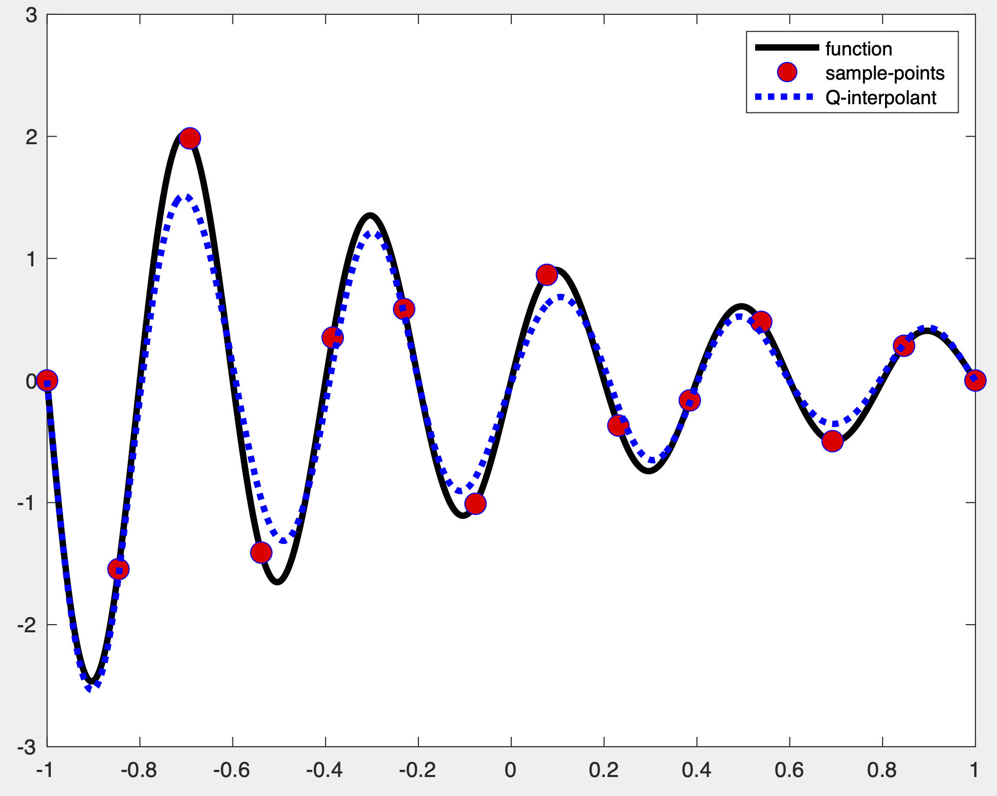
The interface is very intuitive with few example it is easy to practice with the library. Here is a example of quasi-interpolation of a set of points taken from a sampling of a function:

⬇

1 % set the function to be approximated

2 effe = @(x) exp(-x).*sin(5*pi*x);

3 effe1 = @(x) ((5*pi*cos(5*pi*x)) - sin(5*pi*x)).*exp(-x);

4 [a,b] = deal(-1,1); % range of the function

5 d = 4; % degree of quasi interpolant

6 N = 14; % number of sampling points

7 m = 1000; % number of evaluation points for plotting

8 % plot the function

9 xx = linspace(a,b,m); yy = effe(xx);

10 plot( xx, yy, ’LineWidth’, 3, ’Color’, ’black’ );

12 % Sample function and evaluate f and f’ at sample points

13 x = linspace(a,b,N); y = effe(x); yprime = effe1(x);

15 % Create a QIBSH object for 1D quasi-interpolation

16 Q = QIBSH1D(’Qhermite’);

17 % build quasi interpolant for (x,y) data, no cyclic data.

18 Q.build( d, x, y, yprime, false );

20 % plot the sampling points

21 hold on;

22 plot( x, y, ’ob’, ’MarkerSize’, 10, ’MarkerFaceColor’, ’red’ );

24 % plot the approximated interpolant

25 plot( xx, Q.eval( xx ), ’:’, ’LineWidth’, 3, ’Color’, ’blue’ );

26 legend(’function’,’sample-points’,’Q-interpolant’);

The output of the script is shown in Fig. 1.

Refer to caption — Figure 1: Output of quasi-interpolant for function $\mathrm{e}^{-x}\sin(5\pi x)$ with $14$ equally spaced sample points in the interval $[-1,1]$ .

4.3 Procedures for Quasi Interpolation of Function of One Variable

Using the library we can solve the one dimensional problem of Quasi Interpolation. Given the values of a function and of its first derivatives at some points, provided a knot set and the desired spline degree, the user can find the Hermite spline quasi interpolating the data. The final approximation of the $QI^{(BS)}$ is given in terms of its B-spline coefficients. Optionally, function and derivative evaluations can also be returned. When first derivative values are not available, their approximations are first computed and the $QI^{(BSa)}$ quasi-interpolant is used.

In addition, specific procedures for the treatment of periodic functions are available. These functions specializes the QI procedures for the coefficients and for the finite difference scheme, when periodic knots are used.

4.4 Procedures for Tensor Product Quasi Interpolation

The computation of two dimensional BSH QI in the tensor product form follows the scheme from Section 3. For data organized on regular grids, the idea is to split the process into one dimensional problems along the axes directions, quasi interpolating the values of the function and of partial derivatives given in matrix form. When partial derivatives are not available, we combines the tensor product of BSH QI with the finite difference scheme (6). The implementation to reduce the computational costs is based on the computation of $x$ -partial derivatives values of the matrix $\mathbf{F}$ and generating the approximations for $\mathbf{F_{x}}$ . Then, one dimensional QI problems along the $x$ axis are solved storing the coefficients into an auxiliary matrix $\mathbf{D}^{(a)}$ . Now, the approximate derivative of $\mathbf{D}^{(a)}$ are computed and stored in the matrix $\mathbf{D^{\prime}}^{(a)}$ . These two matrices are used for the last step: the solutions of QI problems along the $y$ axis, having $\mathbf{D}^{(a)}$ and $\mathbf{D^{\prime}}^{(a)}$ as inputs, returns the spline coefficients. Computational cost is reduced since the aprroximation of the derivatives are related to two function calls rather than three. Moreover, for the matrix case, the computation of the coefficients $\gamma_{i}^{(n)}$ in (6), and of the matrix $\Gamma^{(l)}$ in (7) is done only once.Finally we remark that also the tensor product case has been generalized and adapted for function domains which can easily be described in polar coordinates in the plane. Hence, we can use the library to compute the QI or derivative approximations for a periodic function $f=f(\rho,\theta)$ of period $T>0$ with respect to its second argument $\theta$ .

In the $m$ D case the quasi interpolant is implemented only when the derivatives are approximated, using a generalization of the 2D procedure. In this case the computational costs remain related to the dimension $m$ . The use of the exact derivatives has a higher computational cost, so it has not be considered.

5 Numerical Tests

5.1 Functions of One Variable

We report the convergence results for the BSH Quasi Interpolant on the test function

f_{1}(x)=e^{-x}\sin(5\pi x)\quad x\in\left[-1,1\right]

(23)

from [Mazzia and Sestini, 2009a]. Numerical examples are performed using the Matlab Toolbox QIBSH++.

The Table 5.1 shows the errors and the estimated orders of convergence of the Quasi Interpolant. For spline degree $d=3$ we apply to the function test the operators $Q_{d}^{(BS)}$ and $Q_{d}^{(BSa)}$ , defined respectively in (2) and (9). For the sake of comparison, we use also a discrete Quasi Interpolant of the same degree $d$ , here denoted as $QIS$ , described in [Sablonnière, 2005] and the spline interpolant spapi from Matlab [MATLAB, 2012]. As usual, $N$ is the number of mesh steps between uniformly spaced $N+1$ spline knots, and errors are estimated by the infinity norm on $1000$ points uniformly spaced in the domain of the functions, the timing $\mathbf{t}$ is computed as the averaged time over $40$ runs (in secs.) for approximating the test functions and evaluating the spline using an Intel Core I7-6500U $2.50$ GHz with Matlab R2020a for Windows ( $64$ bit). The error values confirm the expected rate of convergence for $Q_{d}^{(BS)}$ and $Q_{d}^{(BSa)}$ , as $d+1$ . We also report the convergence behaviour for the operator $QI^{(BS)}$ and $QI^{(BSa)}$ for $d$ ranging between $2$ and $5$ in Figure 3. Moreover, since the described quasi-interpolant operator can also be applied with a non-uniform knot partition, in Figure 4 we show the convergence behavior for this case with the function $f_{2}=\dfrac{e^{-x/s}-e^{(x-2)/s}}{1-e^{-2/s}}$ , and $s=10^{-3/2}$ .

Note that as $N$ increases, the error using $Q_{d}^{(BS)}$ and $Q_{d}^{(BSa)}$ becomes similar, especially for the choice $l=d+1$ . To preserve the order of convergence it is enough to choose $l=d$ , but the part of the error due to the derivative approximation is dominant in this case. These results suggest that the use of $Q_{d}^{(BSa)}$ can be competitive with other DQI interpolants, especially when the approximation of higher order derivatives is required.

\tbl

Convergence Analysis : function $f_{1}$ , spline degree $3$ , GBDF order $4$ . QIBSH QIBSHa $\mathbf{N}$ $\mathbf{Error}$ $\mathbf{Order}$ $\mathbf{t}$ $\mathbf{Error}$ $\mathbf{Order}$ $\mathbf{t}$ 16 1.7×10^-1 $**$ 1.4×10^-5 8.5×10^-1 $**$ 2.4×10^-5 32 8.8×10^-3 4.3 1.6×10^-5 7.3×10^-3 6.9 2.7×10^-5 64 3.1×10^-4 4.8 1.4×10^-5 1.5×10^-4 5.6 2.0×10^-5 128 2.4×10^-5 3.7 1.4×10^-5 1.8×10^-5 3.1 2.4×10^-5 256 9.1×10^-7 4.7 1.8×10^-5 8.3×10^-7 4.4 3.6×10^-5 512 7.5×10^-8 3.6 2.8×10^-5 7.4×10^-8 3.5 6.0×10^-5 1024 4.2×10^-9 4.2 5.3×10^-5 4.2×10^-9 4.1 1.1×10^-4 Matlab QIS $\mathbf{N}$ $\mathbf{Error}$ $\mathbf{Order}$ $\mathbf{t}$ $\mathbf{Error}$ $\mathbf{Order}$ $\mathbf{t}$ 16 5.2×10^-1 $**$ 6.5×10^-4 4.9×10^-1 $**$ 1.3×10^-4 32 1.1×10^-2 5.6 1.2×10^-3 5.1×10^-2 3.3 1.3×10^-4 64 2.6×10^-4 5.3 2.3×10^-3 4.0×10^-3 3.7 1.9×10^-4 128 2.2×10^-5 3.6 3.8×10^-3 2.7×10^-4 3.9 1.3×10^-4 256 9.0×10^-7 4.6 6.1×10^-3 1.6×10^-5 4.1 1.5×10^-4 512 7.5×10^-8 3.6 1.4×10^-2 1.1×10^-6 3.9 1.5×10^-4 1024 4.2×10^-9 4.1 3.3×10^-2 6.5×10^-8 4.0 1.8×10^-4

Moreover, comparing the computational time (expressed in secs.) in the Table 5.1 and in Figure 2 top for $d=3$ and in Figure 2 bottom, for $d=5$ , confirms the efficiency of the QI BSH with respect to the other methods.

5.2 Numerical solution of Boundary Value Problems

The main aim of the library QIBSH is to improve the performance of the Matlab code TOM for the numerical solution of Boundary Value Problems (BVPs) that are assumed to have the first order system form,

y^{\prime}(x)=f(x,y),\quad a\leq x\leq b,

(24)

where $y\in R^{m},f:R\times R^{m}\rightarrow R^{m}$ , with boundary conditions,

g(y(a),y(b))=0.

The first release of the code has been described in [Mazzia and Trigiante, 2004] whereas the update release that include the BS linear multistep method is described in [Mazzia et al., 2009b]. One of the main characteristic of the code is that it implements an hybrid mesh selection based on conditioning. With the inclusion of the BS-scheme the code was able to solve very difficult singularly perturbed BVPs, giving in output a continuous approximation of the solution, but was not able to have an efficient execution time for general problem, the Matlab code spending most of the time in computing the variable coefficients of the linear multistep methods. We do not describe here the new release of the code but we just show how the use of the library QIBSH make this code faster with respect to the original Matlab version and competitive with the Matlab codes bvp4c and bvp5c and the code bvptwp [Cash et al., 2013]. The library has been integrated with the code TOM for both the evaluation of the coefficients of the linear multistep BS method and the evaluation of the continuous extensions, needed for nonlinear problems when the mesh is changed. The quasi-interpolant is also used when the multistep method is the Top Order Method, or another class of Boundary Value Method, as quasi-interpolation scheme.

Here we report some numerical experiment on two singularly perturbed boundary value problems used in [Cash et al., 2013] and available in [Mazzia and Cash, 2015]. We choose two examples in this class that require changes of the mesh in order to compute the numerical solution and need a variable step-size. All the examples in this section have been run using Matlab R2021b on iMac with a 3.6 GHz Intel core i9, 10 core.

The first numerical test chosen is the problem bvpT6, the second is the nonlinear problem bvpT30. Both are singular perturbed problems with a turning point.

We use different values of the parameter $\lambda$ and we select input tolerances $atol=rtol$ as $10^{-3},10^{-4},\cdots,10^{-8}$ . The code TOM is used with the BS method of order 6 and the hybrid mesh selection denoted NSSE [Mazzia, 2022], designed for the solution of non stiff problems. The work precision diagrams are reported in Figures 6-6. The two codes called TOM and TOM_QIBSH++ denote the code TOM with and without the use of the library QIBSH, we compare them with the codes bvp4c, bvp5c, twpbvpc_l, twpbvpc_m and twpbvp_m. The last are some of the available codes in the package bvptwp, the first one use the conditioning in the mesh selection and the Lobatto schemes, the second is based on Monoimplicit Runge-Kutta schemes. It is interesting to see that in all the experiments the use of the library QIBSH reduce considerable the time and make the code TOM comparable with the other available codes. We observe that for the nonlinear problem bvpT30 with parameter $\lambda=10^{-3}$ only the codes with a mesh selection based on conditioning are able to compute a solution. In this case Figure 6 clearly show the efficiency of the code TOM_QIBSH++. Further experiments using the code can been found in [Mazzia and Settanni, 2021, Mazzia, 2022].

5.3 Functions of Two Variables

We use the BSH tensor product on the well known Franke function from the test suite in [Franke, 1982, Renka and Brown, 1999].

\tbl

Convergence Analysis for test function Franke: bivariate tensor product spline of degrees $3\times 3$ GBDF order $4$ . QIBSH QIBSHa $\mathbf{N}$ $\mathbf{Err}$ $\mathbf{Ord}$ $\mathbf{t}$ $\mathbf{Err}$ $\mathbf{Ord}$ $\mathbf{t}$ 16 2.9×10^-3 $***$ 9.6×10^-4 1.8×10^-3 $***$ 9.7×10^-4 32 1.1×10^-4 4.7 9.8×10^-4 1.3×10^-4 3.9 1.0×10^-3 64 5.2×10^-6 4.4 1.1×10^-3 2.2×10^-6 5.9 1.1×10^-3 128 2.9×10^-7 4.1 1.4×10^-3 2.4×10^-7 3.2 1.5×10^-3 256 1.6×10^-8 4.2 2.8×10^-3 1.5×10^-8 4.0 3.6×10^-3 512 1.1×10^-9 3.9 1.1×10^-2 1.1×10^-9 3.8 1.2×10^-2 1024 7.2×10^-11 3.9 4.5×10^-2 7.2×10^-11 3.9 5.7×10^-2 Matlab QIS $\mathbf{N}$ $\mathbf{Err}$ $\mathbf{Ord}$ $\mathbf{t}$ $\mathbf{Err}$ $\mathbf{Ord}$ $\mathbf{t}$ 16 2.1×10^-3 $***$ 4.4×10^-3 9.3×10^-3 $***$ 2.3×10^-3 32 7.9×10^-5 4.7 6.6×10^-3 7.9×10^-4 3.6 2.3×10^-3 64 4.6×10^-6 4.1 9.5×10^-3 5.2×10^-5 3.9 3.2×10^-3 128 2.9×10^-7 4.0 1.8×10^-2 3.4×10^-6 3.9 3.4×10^-3 256 1.6×10^-8 4.2 3.2×10^-2 2.2×10^-7 4.0 7.8×10^-3 512 1.1×10^-9 3.9 9.4×10^-2 1.4×10^-8 4.0 2.6×10^-2 1024 4.1×10^-14 14.7 3.7×10^-1 8.5×10^-10 4.0 8.5×10^-2

The Table 5.3 summarizes the results on the test function for the tensor product spline of degrees $d_{x}=d_{y}=3$ , and the choice $l=d_{x}+1=d_{y}+1$ for the order of the finite difference scheme. Again, we are comparing the behavior of the tensor product formulation of the operators $Q_{d}^{(BS)}$ and $Q_{d}^{(BSa)}$ , to the tensor product of the DQI $QIS$ , and to the one from Matlab spapi. Infinity norm errors are computed against the exact values on a uniform grid of $101\times 101$ points in the unit square. The numerical experiments are carried out on a personal computer Intel Core I7-6500U 2.50GHz with Matlab 2020a for Windows (64 bit).

When fewer knots are available, it is convenient to use the operator $Q_{d}^{(BSa)}$ , choosing at least $l=d$ ¹¹ 1 since in the following tests we always adopt $d_{x}$ = $d_{y}$ , we simplify the notation by using the letter $d=d_{x}=d_{y}$ and denoting the used tensor product of bidegree $d$ .otherwise the error for the first derivatives approximations gets larger. On the contrary, as $N$ increases, and a larger number of knots is available, the user can use a finite difference scheme increasing the approximation order $l$ . Indeed, for $N\geq 256$ , the approximation for BSH gives the same results. In particular they tend to have the same behavior of BSH, as if the partial derivatives values would have been available. The Hermite Quasi Interpolant in these cases has smoothed all the first partial derivative approximating errors. Note that the computational time between $Q^{(BS)}$ and $Q^{(BSa)}$ does not differ so much. In fact, this is due to the efficient approximation for the derivatives, which is not adding any significant computational cost to the one of the QI.
Indeed, comparing the time efficiency of the QIBSH++ tensor product operator to the other interpolants tested, confirms its good behaviour as an approximating method for functions of two variables in terms of goodness of fit and timing. In Figure 7 we also report the work precision diagrams for the Franke function with biddegree $d=3$ and $d=5$ . This motivates once more the use of the Hermite Quasi Interpolant even when partial derivatives are not directly available, a situation often occurring in real applications, as it will be shown later.

Also for the 2D case, we analyze an example where the convergence can benefit from a non uniform mesh partition. In particular, we approximate the Schrek’s first surface $f(x,y)=\displaystyle{\log\left(\frac{\cos(y)}{\cos(x)}\right)}$ restricting our-self to the square domain $\displaystyle{\left[-\frac{\pi}{2}+\eta,\frac{\pi}{2}-\eta\right]^{2}}$ , with $\eta=10^{-2}$ .

As shown in Figure 8, the considered example is a minimal area surface which exhibits a high variation along each side of the definition domain. Therefore, a uniform knot partition will not guarantee a suitable error reduction at the boundary layers. The convergence results are shown in Figure 9 also considering the spline bidegree $d$ varying from $2$ to $5$ .

5.4 Surface parameterization with high smoothness for complex geometries

In this example we demonstrate how the tensor product BSH QI can be useful to produce spline parameterizations of complex geometries with the desired smoothness in any direction. We construct a complex geometric model by assembling together three primitive shapes: hollow hemisphere, cylinder and conical frustum. The resulting object is a glass geometry shape, see Figure 10. In order to construct a continuous spline approximation of the considered object we need to reparametrize every shape in such a way to obtain conforming parameter domains. More in detail, we consider a hollow hemisphere $S$ with radius $r=2$ described by a parameterization $F_{S}(\theta,\phi):\Omega_{S}\rightarrow S$ with $\Omega_{S}:=[0,2\pi]\times[-\pi,-0.2)$ with the following coordinates representation:

	$\displaystyle X_{S}=$	$\displaystyle r\cos(\theta)\sin(-\phi);$
	$\displaystyle Y_{S}=$	$\displaystyle r\sin(\theta)\sin(-\phi);$
	$\displaystyle Z_{S}=$	$\displaystyle r\cos(\phi).$

We consider only the values for $Z_{S}>0$ . The cylinder $C$ considered here can be described by the following $F_{C}(\theta,h):\Omega_{C}\rightarrow C$ , with $\Omega_{C}=[0,2\pi]\times[-0.2,6]$ . The physical coordinates can be expressed as:

	$\displaystyle X_{C}=$	$\displaystyle~r_{C}\cos(\theta);$
	$\displaystyle Y_{C}=$	$\displaystyle~r_{C}\sin(\theta);$
	$\displaystyle Z_{C}=$	$\displaystyle~\frac{(6-r\cos(-0.2))}{(6+0.2)}(h+0.2)+r\cos(-0.2);$

with $r=2$ and $r_{C}=r\sin(0.2)$ . Finally the conical frustum $V$ is defined with $F_{V}(\theta,v):\Omega_{V}\rightarrow V$ , with $\Omega_{V}=[0,2\pi]\times(6,10]$ . The physical coordinates are computed as:

X_{V}=a\frac{v\cos(\theta)}{10};\qquad Y_{V}=a\frac{v\sin(\theta)}{10};\qquad Z_{V}=v;

with $a$ uniformly varying from $|r_{c}h_{f}|/6$ to $3$ . The three shapes are parameterized in such a way that the resulting geometries can be physically joined with $C^{0}$ continuity and their parameter domains can be assembled to form a unique domain $\Omega$ defined as: $\Omega=\Omega_{S}\cup\Omega_{C}\cup\Omega_{V}$ where we define our quasi-interpolant spline approximation $F$ . In this case $\Omega=[0,\pi]\times[-\pi,10]$ . If we are interested in constructing a $C^{0}$ representation $F$ , at this stage we only need to call the constructor for the 2D object QIBSH and we can compute a spline representation $F$ with a chosen bidegree $d$ , periodic along with the first direction, by approximating the $F_{x}$ , $F_{y}$ and $F_{xy}$ with a finite difference scheme of order $\ell=\max\{d_{x},d_{y}\}+1$ . Although the resulting surface has in principle $C^{d-1}$ smoothness, its derivatives might present sharp variation and/or unwanted oscillations, see Figure 11, left, where we plotted the first derivative profile with respect to the $y$ direction. To get an improved parametric representation, we therefore proceed as follows. Firstly the desired smoothness for the final approximation $F$ is fixed. For practical purposes we limit our-self to the case of constructing a $C^{1}$ spline parameterization. Hence, the chosen degree should be $d_{x},d_{y}\geq 2$ . Secondly, since for this example the derivatives with respect to $x$ direction are almost zero, we will tackle only the derivatives with respect to the $y$ direction.

The proposed algorithm can be summarized with the following steps,

(1)

A discrete approximation $\tilde{F}_{yy}$ of the second derivatives in the $y$ direction is constructed, by using finite centered differences.
(2)

A continuous model of $\tilde{F}_{yy}$ is provided by applying the $Q^{(BSa)}$ operator, thus obtaining $\tilde{F}_{yy}\approx QA_{yy}$ .
(3)

The first derivative $QA_{y}$ in $y$ direction is now computed as,

$QA_{y}(\hat{x},y_{z}):=\int_{c}^{y_{z}}QA_{yy}(\hat{x},z)\,dz,$

where $y_{z},\,z=0,\ldots,M$ , knots of the mesh.

The output of this procedure can be seen in Figure 11, right. We can visually appreciate how the function results more regularized. Some oscillations are still visible, in fact, the steps (1)-(3) can be performed by starting from any order of derivation and then can be backward iterated till the computation of the approximant surface for the original one.

5.5 Functions of three Variables

We consider the following volume:

\displaystyle f(x,y,z)=\frac{\sqrt{64-81((x-1/2)^{2}+(y-1/2)^{2}+(z-1/2)^{2})}}{9}-\frac{1}{2}\quad x,y,z\in[0,1].

In Table 5.5 we report the maximum error and the estimated order of convergence for the operator $Q_{d}^{(BSa)}$ , by varying the used degree $d$ for each direction and the number of mesh steps $N$ between uniformly spaced $N+1$ knots. In the following test $d_{x}=d_{y}=d_{z}=d$ and the approximation order $\ell$ for the derivatives is computed as $d+1$ for $d$ odd and as $d+2$ for $d$ even, in order to produce a symmetric output in line with the original function $f$ . The order of convergence $d+1$ is reached in all the considered cases.

\tbl

Convergence Analysis for the volume $f$ in Section 5.5. QIBSHa $d=2$ QIBSHa $d=3$ QIBSHa $d=4$ QIBSHa $d=5$ $\mathbf{N}$ $\mathbf{Err}$ $\mathbf{Ord}$ $\mathbf{Err}$ $\mathbf{Ord}$ $\mathbf{Err}$ $\mathbf{Ord}$ $\mathbf{Err}$ $\mathbf{Ord}$ 16 2.3×10^-3 $**$ 1.7×10^-3 $**$ 9.5×10^-4 $**$ 9.6×10^-4 $**$ 32 3.7×10^-4 2.6 2.7×10^-4 2.7 1.1×10^-4 3.1 1.2×10^-4 3.1 64 2.8×10^-5 3.8 1.6×10^-5 4.1 4.4×10^-6 4.7 4.3×10^-6 4.7 128 1.9×10^-6 3.9 5.8×10^-7 4.8 8.8×10^-8 5.6 6.7×10^-8 6.0 256 2.8×10^-7 2.8 1.4×10^-8 5.4 3.1×10^-9 4.9 9.2×10^-10 6.2

5.6 Real World Data Tests

In this Section we report two real applications where the use of the library QIBSH gave interesting results and improvements with respect to other usual techniques.

5.6.1 Continuous Digital Elevation Models

We consider data-sets available to produce Digital Elevation Models (DEM). DEM is a digital model or a 3D representation of a terrain’s surface altitude with respect to the mean sea level. Technically DEM contains only the elevation information without taking into account possible vegetation, buildings, or other types of objects. DEM are generated by using the elevation information from points spaced either at regular or irregular intervals. In the first case, when the points are collected in regular grids, we talk about raster DEM, in the latter case, the points are arranged in triangular irregular networks, hence, we refer to vector DEM. In this example we use the NASADEM²² 2 NASA JPL (2021). NASADEM Merged DEM Global 1 arc second V001. Distributed by OpenTopography. https://doi.org/10.5069/G93T9FD9Accessed:2021-08-22dataset: a modernization of Global Digital Elevation Models. The satellite data are preprocessed according to several optimization and interpolation algorithms and they are provided in grid form. NASADEM products are freely available through the Land Processes Distributed Active Archive Center (LP DAAC) at $1$ arc-second spacing ( $\sim 30$ meters). Data were collected from February 11, 2000 to February 22, 2000. In order to produce a continuous model of the discrete dataset, since the given samples are uniformly spaced (raster DEM), it is reasonable to adopt a tensor product approach. In addition, the produced continuous model should still be able to capture the abrupt changes in the terrain shape, so it is reasonable to require up to $C^{2}$ smoothness.

Among the many application of DEM a continuous model might be used for 3D rendering visualization purposes, hydrological and geomorphological investigations, rectification of satellite imagery, terrain correction and so on.

In this example we select a terrain matrix of size $1197\times 2347$ in the Italian Appenini mountain region, see Fig. 12. In Table 5.6.1 we report the root mean square error (RMSE) and the normalized RMSE (NRMSE) on the quasi-interpolation nodes.

\tbl

RMSE and NRMSE on the quasi-interpolation nodes. QIBSHa QIBSHa $d=2$ $d=3$ RMSE 6.32×10^-1 7.54×10^-2 NRMSE 4.22×10^-4 5.03×10^-5

Since usually DEM involve a large amount of data, downsampling is a widely used technique to reduce the storage requirements. Our goal is to construct a quasi-interpolant spline surface on half of the given data, and then to evaluate the produced output on the other half of samples. The obtained results are compared with the available Matlab routines for gridded interpolation: linear, cubic, nearest neighbour (N-N), cubic spline (Spline), modified Akima (M-Akima). The RMSE and the NRMSE are reported in Table 5.6.1.

\tbl

RMSE and NRMSE results for the downsampling DEM, comparisons with the available Matlab routines.. Linear Cubic Spline $\mathbf{N}$ -N M-Akima QIBSHa QIBSHa $d=1$ $d=3$ $d=3$ $d=0$ $d=3$ $d=2$ $d=3$ RMSE 2.63 2.10 2.04 8.97 2.13 1.85 2.05 NRMSE 1.76×10^-3 1.41×10^-3 1.36×10^-3 6.00×10^-3 1.42×10^-3 1.23×10^-3 1.37×10^-3

5.6.2 Curvature Inpainting of Corneal Topographer Data with Missing Regions

We present another application of the tensor product BSH QI to a real problem. The main goal here is to recover the elevation and the radial curvature data of a real eye, processing data with missing points. Sometimes during the topographer acquisition phase it is impossible to detect data points in some regions: these are called inpainting regions and have to be filled in by some numerical techniques. We apply the TV-H^-1 inpainting model [Burger et al., 2009, Schönlieb and Bertozzi, 2011], implemented in the Matlab function bvnegh_inpainting_convs[Schönlieb, 2011]. Applying only this inpainting model to the elevation data was not so succesfull, hence we apply it to the radial curvature values, combining it with a regularizing phase given by the BSH QI interpolant. We start from the elevation data of the surface in the regions where they are available, we approximate the radial curvature, and then apply digital inpainting to the curvature values with missing data. The curvature is computed along each radial direction approximating the radial partial derivatives using the scheme (6). After the curvature of the missing regions is recovered using the TV-H^-1 inpainting, the elevations data of the eye are computed radially, solving a second order ODE. The tensor product of the BSH QI is applied using its polar coordinates form, when, during a final step, we regularize the final eye surface. Extended discussion, details and numerical results can be found in [Andrisani et al., 2019].

6 Conclusions

The C++ library QIBSH++ for the approximate solution of several applicative problems provides the implementation of a Hermite type quasi-interpolant operator, with the possibility to approximate the derivatives, with finite difference methods, when they are not available. A brief discussion on the theoretical convergence properties of the method is included, together with some implementation details. Numerical tests show the convergence properties of the method, even when derivatives are not available and they are approximated. Computational times and approximation errors make the BSH QI method competitive with other well-known interpolations and quasi interpolation methods. Moreover, the use of the Matlab C-MEX interfaces for some QIBSH++ procedures, leads to performance optimization of the code TOM in terms of computational time. The use of the library is also suggested in several applicative fields when high smoothness and high degree splines are required.

7 Acknowledgments

The research of Antonella Falini is founded by PON Project AIM 1852414 CUP H95G18000120006 ATT1. The authors Antonella Falini and Francesca Mazzia thank the Italian National Group for Scientific Computing (Gruppo Nazionale per il Calcolo Scientifico) for its valuable support under the INDAM-GNCS project CUP_E55F22000270001.

References

[Andrisani et al., 2019] Andrisani, A., Mininni, R. M., Mazzia, F., Settanni, G., Iurino, A., Tangaro, S., Tateo, A., and Bellotti, R. (2019). Applications of pdes inpainting to magnetic particle imaging and corneal topography. Opuscula Mathematica, 39(4):453–482.
[Brugnano and Trigiante, 1998] Brugnano, L. and Trigiante, D. (1998). Solving Differential Problems by Linear Multistep Initial and Boundary Value Methods. Stability and Control Ser.: Theory, Methods and Applications. Gordon and Breach.
[Burger et al., 2009] Burger, M., He, L., and Schönlieb, C. (2009). Cahn-Hilliard inpainting and a generalization for grayvalue images. SIAM Journal on Imaging Sciences, 2(4):pp. 1129–1167.
[Burkowski and Hoskins, 1973] Burkowski, F. J. and Hoskins, W. (1973). Algorithm 461: cubic spline solutions to a class of functional differential equations. Communications of the ACM, 16(10):635–637.
[Cash et al., 2013] Cash, J. R., Hollevoet, D., Mazzia, F., and Nagy, A. (2013). Algorithm 927: the matlab code bvptwp.m for the numerical solution of two point boundary value problems. ACM Transactions on Mathematical Software (TOMS), 39(2):1–12.
[Davydov and Zeilfelder, 2005] Davydov, O. and Zeilfelder, F. (2005). TSFIT package. http://personal.strath.ac.uk/oleg.davydov/tsfit/index.html.
[de Boor, 1972] de Boor, C. (1972). On calculating with $B$ -splines. J. Approximation Theory, 6:pp. 50–62.
[de Boor, 1976] de Boor, C. (1976). Splines as Linear Combinations of B-splines: A Survey. MRC technical summary report: Mathematics Research Center. Defense Technical Information Center.
[de Boor, 2001] de Boor, C. (2001). A practical guide to splines, volume 27 of Applied Mathematical Sciences. Springer-Verlag, New York.
[De Falco et al., 2011] De Falco, C., Reali, A., and Vázquez, R. (2011). Geopdes: a research tool for isogeometric analysis of pdes. Advances in Engineering Software, 42(12):1020–1034.
[Dierckx, 1993] Dierckx, P. (1993). FITPACK package. http://www.netlib.org/dierckx/.
[Elber, 1990] Elber, G. (1990). IRIT. https://www.cs.technion.ac.il/ irit/.
[Falini et al., 2022] Falini, A., Mazzia, F., and Sestini, A. (2022). Error estimates for spline BS Hermite Quasi-Interpolation. in preparation.
[Franke, 1982] Franke, R. (1982). Scattered data interpolation: Tests of some method. Mathematics of Computation, 38(157):pp. 181–200.
[Grimstad et al., 2015] Grimstad, B. et al. (2015). SPLINTER: a library for multivariate function approximation with splines. http://github.com/bgrimstad/splinter. Accessed: 2015-05-16.
[Iurino, 2014] Iurino, A. (2014). BS Hermite Quasi-Interpolation Methods for Curves and Surfaces. PhD thesis, Dipartimento di Matematica, Università degli Studi di Bari.
[Iurino and Mazzia, 2013] Iurino, A. and Mazzia, F. (2013). The c library qibsh for hermite quasi interpolation of curves and surfaces. Technical Report 11, Department of Mathematics, University of Bari ALDO MORO.
[Jüttler et al., 2014] Jüttler, B., Langer, U., Mantzaflaris, A., Moore, S. E., and Zulehner, W. (2014). Geometry+ simulation modules: Implementing isogeometric analysis. PAMM, 14(1):961–962.
[Kolda and Bader, 2009] Kolda, T. G. and Bader, B. W. (2009). Tensor decompositions and applications. SIAM Review, 51(3):455–500.
[Mantzaflaris, 2019] Mantzaflaris, A. (2019). An overview of geometry plus simulation modules. In International Conference on Mathematical Aspects of Computer and Information Sciences, pages 453–456. Springer.
[MATLAB, 2012] MATLAB (2012). version 7.14.0 (R2012a). The MathWorks Inc., Natick, Massachusetts.
[Mazzia, 2022] Mazzia, F. (2022). Mesh selection strategies of the code tom for boundary value problems. Annali dell’Università di Ferrara. submitted.
[Mazzia and Cash, 2015] Mazzia, F. and Cash, J. R. (2015). A fortran test set for boundary value problem solvers. AIP Conference Proceedings, 1648(1):020009. website:https://archimede.dm.uniba.it/~bvpsolvers/testsetbvpsolvers/.
[Mazzia and Sestini, 2009a] Mazzia, F. and Sestini, A. (2009a). The BS class of Hermite spline quasi-interpolants on nonuniform knot distributions. Bit Numerical Mathematics, 49(3):pp. 611–628.
[Mazzia and Sestini, 2009b] Mazzia, F. and Sestini, A. (2009b). The BS class of hermite spline quasi-interpolants on nonuniform knot distributions. BIT, 49(3):611–628.
[Mazzia and Sestini, 2012] Mazzia, F. and Sestini, A. (2012). Quadrature formulas descending from BS Hermite spline quasi-interpolation. Journal of Computational and Applied Mathematics, 236(16):4105–4118.
[Mazzia et al., 2006a] Mazzia, F., Sestini, A., and Trigiante, D. (2006a). B-spline linear multistep methods and their continuous extensions. SIAM J. Numer. Anal., 44(5):1954–1973 (electronic).
[Mazzia et al., 2006b] Mazzia, F., Sestini, A., and Trigiante, D. (2006b). BS linear multistep methods and their continuous extensions. SIAM Journal on Numerical Analysis, 44(5):1954–1973.
[Mazzia et al., 2006c] Mazzia, F., Sestini, A., and Trigiante, D. (2006c). BS linear multistep methods on non-uniform meshes. JNAIAM J. Numer. Anal. Indust. Appl. Math, 1(1):131–144.
[Mazzia et al., 2009a] Mazzia, F., Sestini, A., and Trigiante, D. (2009a). The continuous extension of the B-spline linear multistep methods for BVPs on non-uniform meshes. Applied Numerical Mathematics, 59(3-4):723–738.
[Mazzia et al., 2009b] Mazzia, F., Sestini, A., and Trigiante, D. (2009b). The continuous extension of the B-spline linear multistep methods for BVPs on non-uniform meshes. Applied Numerical Mathematics, 59(3-4):723–738.
[Mazzia and Settanni, 2021] Mazzia, F. and Settanni, G. (2021). Bvps codes for solving optimal control problems. Mathematics, 9(20).
[Mazzia and Trigiante, 2004] Mazzia, F. and Trigiante, D. (2004). A hybrid mesh selection strategy based on conditioning for boundary value ODE problems. Numer. Algorithms, 36(2):169–187.
[Pew et al., 2016] Pew, J., Li, Z., and Muir, P. (2016). Algorithm 962: Bacoli: B-spline adaptive collocation software for pdes with interpolation-based spatial error control. ACM Transactions on Mathematical Software (TOMS), 42(3):1–17.
[Renka and Brown, 1999] Renka, R. and Brown, R. (1999). Algorithm 792: accuracy test of ACM algorithms for interpolation of scattered data in the plane. ACM Transactions on Mathematical Software (TOMS), 25(1):78–94.
[Renka, 1993] Renka, R. J. (1993). Algorithm 716: Tspack: Tension spline curve-fitting package. ACM Transactions on Mathematical Software (TOMS), 19(1):81–94.
[Renka, 2009] Renka, R. J. (2009). Algorithm 893: Tspack: tension spline package for curve design and data fitting. ACM Transactions on Mathematical Software (TOMS), 36(1):1–8.
[Sablonnière, 2005] Sablonnière, P. (2005). Univariate spline quasi-interpolants and applications to numerical analysis. Rend. Semin. Mat. Univ. Politec. Torino, 63(3):211–222.
[Schönlieb, 2011] Schönlieb, C. (2011). Higher-order total variation inpainting. http://it.mathworks.com/matlabcentral/fileexchange/34356-higher-order-total-variation-inpainting.
[Schönlieb and Bertozzi, 2011] Schönlieb, C. and Bertozzi, A. (2011). Unconditionally stable schemes for higher order inpainting. Communications in Mathematical Sciences, 9(2):pp. 413–457.
[Schumaker, 2018] Schumaker, L. (2018). SPLINEPAK. https://archive.siam.org/books/ot142/.
[Schumaker, 2007] Schumaker, L. L. (2007). Spline functions: basic theory. Cambridge Mathematical Library. Cambridge University Press, Cambridge, third edition.
[Vázquez, 2016] Vázquez, R. (2016). A new design for the implementation of isogeometric analysis in octave and matlab: Geopdes 3.0. Computers & Mathematics with Applications, 72(3):523–554.
[Walker et al., 2019] Walker, P., Krohn, U., and Carty, D. (2019). Arbtools: A tricubic spline interpolator for three-dimensional scalar or vector fields. Journal of open research software., 7(1):12.

The Object Oriented C++ library QIBSH++ for Hermite spline Quasi Interpolation

Abstract

Keywords:

category

keywords

1 Introduction

2 BSH Quasi Interpolants in One Dimension

3 BSH Quasi Interpolants and Tensor Product

Remark 3.1

4 Implementation Details

4.1 C++ classes

4.2 Matlab classes

4.3 Procedures for Quasi Interpolation of Function of One Variable

4.4 Procedures for Tensor Product Quasi Interpolation

5 Numerical Tests

5.1 Functions of One Variable

5.2 Numerical solution of Boundary Value Problems

5.3 Functions of Two Variables

5.4 Surface parameterization with high smoothness for complex geometries

5.5 Functions of three Variables

5.6 Real World Data Tests

5.6.1 Continuous Digital Elevation Models

5.6.2 Curvature Inpainting of Corneal Topographer Data with Missing Regions

6 Conclusions

7 Acknowledgments

References